Continuous-time optimal control for trajectory planning under uncertainty

Abstract

This paper presents a continuous-time optimal control framework for the generation of reference trajectories in driving scenarios with uncertainty. A previous work [1] presented a discrete-time stochastic generator for autonomous vehicles; those results are extended to continuous time to ensure the robustness of the generator in a real-time setting. We show that the stochastic model in continuous time can capture the uncertainty of information by producing better results, limiting the risk of violating the problem’s constraints compared to a discrete approach. Dynamic solvers provide faster computation and the continuous-time model is more robust to a wider variety of driving scenarios than the discrete-time model, as it can handle further time horizons, which allows trajectory planning outside the framework of urban driving scenarios.

1 Introduction

The development of autonomous vehicles is a core research interest in the automotive industry and aims to meet the numerous challenges of the transport sector. Autonomous vehicle decision-making problems represent a vast research field and trajectory planning is one of its intrinsic components. The constraints over the dynamics of the vehicle must consider the safety, performance and comfort of the passenger in the proposed solutions.

The simulations of autonomous vehicles cannot reproduce the complexity of a real-life environment with the range of possibilities of unexpected events. Furthermore, complex systems embed complex components interacting between themselves and each of them can be responsible for a drawback in the nominal functioning. The noise of a sensor, a false measurement due to weather conditions or a technical failure can affect the safeness of the user.

Therefore, a stochastic component in the model can be a way for the software to anticipate errors due to hardware components and unpredictable events in the environment. Safety is a significant concern in autonomous vehicles and the capacity to model the mistakes in various driving scenarios addresses this issue. As one cannot design all real-life scenarios for anticipation, simulators must accurately reproduce the most common situations from road traffic. In trajectory planning, a reference trajectory is used as a benchmark to compare with the simulated path of the vehicle.

This paper proposes a continuous-time optimal control problem for generating reference trajectories addressed to autonomous vehicles. The following parts are divided as follows: Section 2 depicts an overview of the literature, tackling the current challenges in trajectory planning and optimal control problems, Section 3 emphasises the continuous-time optimal control problem with chance constraints and Section 4 is a comparison of different configurations and their performances. It shows the continuous-time model performs better than the discrete-time model, as it computes faster and the solver finds solutions for trajectory planning over far horizons, which are helpful on high-speed driving scenarios. Finally, Section 5 concludes our study and opens it to further research.

2 Related Work

The trajectory planning problem for autonomous and semi-autonomous vehicles has been studied through various frameworks as the interest in this problem grew within several research fields.

Optimal control with constraints has been adopted since 2010 [2] as it enables obtaining a model considering the bounds of the environment and measuring the level of threats depending on the vehicle’s current state. Various models have been developed for modelling vehicles, among them the unicycle and 4-wheeled models, which are broadly studied nowadays in both robotics [3] [4] and autonomous vehicles [5] researches. Extending advances in robotics research to autonomous vehicles opened several aspects of research, such as guidance [6] and trajectory predictions [7]. Those aspects deal with the challenges of road traffic for the navigation of vehicles in real-life conditions.

In particular, safety constitutes one of the main concerns of intelligent vehicle navigation [8] and new researches are carried out with the adoption of several new approaches. The complexity of the environment of real-life navigation involves considering uncertainties, often treated by including a stochastic component in the modelling. Recent research in the literature [9] [10] [11] describes it. This line of research is motivated by the desire to have a model that can capture this stochastic component and include it in the vehicle’s control to assess the safety level more precisely and address the vehicle’s performance. The overview [12] describes several approaches explored in the literature: game theory, probability, Partially Observable Markov Decision Processes (POMDP) and learning. Various research fields show pros and cons when dealing with autonomous vehicle problems.

Neural networks have been used to capture information with the most recent approach based on deep reinforcement learning [13], allowing the neural network to model the uncertainty of the environment and constraints. While this approach captures much information, the computational cost is high. Using deep learning methods to fit real-life contexts is a tough challenge. In autonomous vehicles, embedded systems are used to learn about the environment, but the computation cost can be too high to handle. Therefore, tackling the problem of simulating a driving scenario and performing trajectory planning in real-life conditions should consider those hardware constraints, better handled by other simulation methods.

Optimisation methods with chance constraints are advantageous as the model is sufficiently robust for giving a feasible solution and respecting a good level of approximation. Recent research [9] [1] presents advances in modelling uncertainty using this framework. The article [9] proposes a Gaussian mixture model for uncertainty, allowing convexity properties over the chance constraints to ensure tractability. The authors present simulations with multimodal uncertain obstacles for the trajectory planning of the vehicle, with general polyhedral geometric forms. Previous work in [1] deals with a constrained non-linear optimisation problem for generating reference trajectories, with scenarios including an ego vehicle to control and a third-party target vehicle. In both works, the optimisation problems are formulated in discrete time.

In most cases, as stated in the introduction of [14], discrete-time models are derived from approximations of continuous-time models. The interest in tackling discrete-time optimal control problems is to adapt to real-world applications, where numerical sensors are widely used compared to analog sensors. Furthermore, some stability results are guaranteed in discrete-time and do not hold for continuous-time edge cases, so it guarantees better stability in the control of systems. Ensuring the stability of some continuous-time frameworks is challenging. Still, they are more representative of real-life settings than discrete-time models, so the choice of model should be addressed regarding the context of the problem tackled.

3 Problem Formulation

3.1 Driving scenario

This section presents a generalisation in continuous time from the previous work in [1]. We consider driving scenarios providing information about the trajectory of the vehicles and their environments. This includes other vehicles on the roads and potential obstacles, such as pedestrians. All driving scenarios are defined for a given time horizon.

The prerequisites we consider to be known from the environment to define a driving scenario are the following :

• As in discrete-time, if we consider $n$ vehicles on the road, for $i\in[|1,n|]$, the trajectory of the $i$th vehicle at time $t$ is represented by its Cartesian coordinates $X_{i}(t),Y_{i}(t)$.

• The centre lane of the road is a continuous curve represented by its Cartesian coordinates $(x,C(x))_{x\in\mathbb{R^{+}}}$.

• Likewise, the boundaries of the road are represented by $(x,B(x))_{x\in\mathbb{R^{+}}}$.

• We define a maximum speed allowed by regulations on the road, denoted by $v_{max}$.

Those elements are the minimum amount of information needed to define a driving scenario. Nonetheless, the reference trajectory needs slightly more input. As in the discrete-time case in [1], some additional constraints are also considered:

• The initial state of the ego vehicle to control: $z_{0}$.

• A predefined waypoint for anticipating the next actions to undertake. This can take into account lane change, overtaking or steady driving. Our study considers waypoints defined from the centre lane only for simplicity. See Remark 1.

• An optimality criterion to define, here represented by a cost function.

• Additional constraints of the vehicle for considering the passenger’s comfort. Those constraints are both cinematic and dynamic.

3.2 Optimal control problem

Let’s recall the formulation of the optimal control problem as in [1] :

• $z(t)$ the control states variable, with $z(t)\in\mathcal{Z}$ and $\mathcal{Z}$ the feasible set of states. $z_{\textrm{init}}$ and $z_{\textrm{term}}$ are initial and terminal states of the system ;

• $u(t)$ the optimal control input, with $u(t)\in\mathcal{U}$ and $\mathcal{U}$ the feasible set of control inputs ;

• $t_{0}$ and $t_{n}$ are initial and final time ;

• $\ell(\cdot)$ the objective function to minimise ;

• $f(\cdot)$ the function designing the system dynamics of the control state $z(t)$ ;

• $c(\cdot)$ is the inequality constraint function.

The optimal control problem is then given by :

$$\begin{aligned} \underset{z(\cdot),u(\cdot)}{\textrm{min}}\quad&\int_{t_{0}}^{t_{n}}\ell(z(t),\ u(t))dt\\ \textrm{s.t.}\quad&\dot{z}(t)=f(z(t),u(t)),\\ &c(z(t),u(t))\leq 0,\\ &z\left(t_{0}\right)=z_{\textrm{init}},\quad z\left(t_{n}\right)=z_{\textrm{term}},\\ &z(t)\in\mathcal{Z},\quad u(t)\in\mathcal{U}.\end{aligned}$$ (1)

Continuous-time optimal control problems can be solved by discretising the integral form of the problem, as it has been done in [1]. In this study, our goal is to show the performances of dynamic simultaneous control on the reference trajectory generation, compared to the discretised version of the problem which is solved as a constrained non-linear optimisation problem.

3.3 Modelling a reference trajectory generator

The choices for modelling the vehicle align with the discrete-time problem tackled in [1]. The unicycle kinematic model gives the following state of the ego vehicle at time $t$:

$$z_{t}=[x_{t},y_{t},\theta_{T},v_{T}]^{T}$$

where $x_{t}$ is the longitudinal position, $y_{t}$ is the lateral position, $\theta_{t}$ is the heading angle of the vehicle and $v_{t}$ is the linear speed. The control input at time $t$ is given by

$$u_{t}=[a_{t},\omega_{t}]$$

where $a_{t}$ is the linear acceleration and $\omega_{t}$ is the angular velocity. The ego vehicle’s control-state relationship is given by :

$$\begin{aligned} \frac{dz_{t}}{dt}=f(z_{t},u_{t})\end{aligned}$$ (2)

where $f(z_{t},u_{t})=[v_{t}\cos(\theta_{t}),v_{t}\sin(\theta_{t}),\omega_{t},a_{t}]^{T}$. The optimal control problem proposed for the reference trajectory generation is the following :

$$\min_{\mathbf{u},\mathbf{z}}\quad \int_{0}^{T}\mathbf{w}_{g}*D^{2}_{t}(x_{t},y_{t})+\mathbf{w}_{v}*(v_{r}-v_{t})^{2}+\mathbf{w}_{a}*a^{2}_{t}$$

$$+\mathbf{w}_{\omega}*\omega^{2}_{t}+\mathbf{w}_{j}*\biggl{(}\frac{da_{t}}{dt}\biggl{)}^{2}+\mathbf{w}_{h}*H(\theta_{t})^{2}$$

$$+\mathbf{w}_{p}*P(x^{tgt}_{t},y^{tgt}_{t},x_{t},y_{t})\hskip 2.84544ptdt$$ (3)

s.t. $$\frac{dz_{t}}{dt}=f(z_{t},u_{t})\hskip 2.84544ptdt,$$ (3.3a)

$$L(x_{t},y_{t})<=0,$$ (3.3b)

$$|v_{t}|\leq v_{max},$$ (3.3c)

$$|\omega_{t}|\leq\omega_{max},$$ (3.3d)

$$|a_{t}|\leq a_{max},$$ (3.3e)

$$\biggl{|}\frac{da_{t}}{dt}\biggl{|}\leq j_{max},$$ (3.3f)

$$K(x^{tgt}_{t},y^{tgt}_{t},x_{t},y_{t})\geq d_{min}$$ (3.3g)

With $\mathbf{u}$ and $\mathbf{z}$ vectors representing the input control and the system’s state, respectively.

The objective function (3.3) comprises a sum of weighted quantities with terms to control the ego vehicle. The weights are chosen as a trade-off between the comfort and security of the passenger and speedness of the vehicle.

• $D_{t}^{2}(x_{t},y_{t})$ is the distance to the waypoint at instant $t$. This term is responsible for controlling the vehicle on the centre line.

• $(v_{r}-v_{t})^{2}$ is the L2-distance to the recommended speed value $v_{r}$, considered as a known input parameter.

• $a^{2}_{t}$ and $\omega^{2}_{t}$ are penalisation terms for the components of the control input $u_{t}$, so the values do not become too large, which can make the control unstable.

• $\bigl{(}\frac{da_{t}}{dt}\bigl{)}^{2}$ is the jerk term. Minimising this quantity allows the vehicle to perform smooth accelerations, which does not make the journey uncomfortable for the passenger.

• $H(\theta_{t})^{2}$ is the distance between the heading angle of the vehicle and the degree of curvature of the centre lane, known as a waypoint.

• $P(x^{tgt}_{t},y^{tgt}_{t},x_{t},y_{t})$ is a potential field function useful to regulate the speed of the ego vehicle towards its distance to the target vehicle. This term models the vehicle’s Adaptive Cruise Control (ACC) [15] feature.

Remark 1

The waypoints $(x^{waypoint}_{t},y^{waypoint}_{t},\theta^{waypoint}_{t})_{t\geq 0}$ are derived from the center lane coordinates directly. Waypoint planning challenges are not tackled in our study.

The constraints cover several aspects of the modelling:

• The constraint (a) is the control-state relationship (2) derived from the unicycle kinematic model.

• $L(x_{t},y_{t})$ is the distance between the coordinates of the ego vehicle and the limits of the road defined in constraint (b). It guarantees the vehicle will stay within the boundaries of the environment.

• The constraint (c) is the maximum linear speed limit of the vehicle

• The constraint (d) is the maximum angular speed limit of the vehicle

• The constraint (e) is the maximum linear acceleration limit of the vehicle

• The constraint (f) is the maximum jerk limit of the vehicle. Even if this term represents comfort for the passenger, a value that is too large could also be dangerous for both the passenger and the vehicle.

• $K(x^{tgt}_{t},y^{tgt}_{t},x_{t},y_{t})$ is the distance between ego and target vehicles defined in constraint (g). To prevent collisions, it guarantees a minimum distance $d_{min}$ between vehicles to prevent collisions.

3.4 Stochastic model

Our stochastic model corresponds to its discrete-time equivalent [1]. Let’s suppose $(x^{tgt}_{t})$ and $y^{tgt}_{t}$ are sampled from Gaussian processes such as :

$$x^{tgt}_{t}\sim\mathcal{N}(\mu_{x_{t}},\sigma_{x_{t}})$$ (4)

$$y^{tgt}_{t}\sim\mathcal{N}(\mu_{y_{t}},\sigma_{y_{t}})$$ (5)

Then, the results from [1] hold. We derive our stochastic model from the deterministic model with a modified constraint (g). Let $K(x_{1},x_{2},x_{3},x_{4})=|x_{1}-x_{2}+x_{3}-x_{4}|$. Therefore, the constraint (g) is replaced by the stochastic constraints (7) and (8).

$$\forall t,\ \mathbb{P}(|x^{tgt}_{t}-x_{t}+y^{tgt}_{t}-y_{t}|\geq d_{min})\geq\alpha\implies$$ (6)

$$\forall t,\ x_{t}+y_{t}\leq\mu_{x_{t}}+\mu_{y_{t}}+d_{min}+\sqrt{\sigma_{x_{t}}^{2}+\sigma_{y_{t}}^{2}}\cdot F_{N}^{-1}(\alpha/2)$$ (7)

$$\forall t,\ x_{t}+y_{t}\geq\mu_{x_{t}}+\mu_{y_{t}}-d_{min}+\sqrt{\sigma_{x_{t}}^{2}+\sigma_{y_{t}}^{2}}\cdot F_{N}^{-1}(1-\alpha/2)$$ (8)

4 Numerical Experiments

The numerical experiments aim to show the efficiency of the continuous-time model compared to previous discrete-time results [1]. The optimal control problem (3.3) is solved with Python Package GEKKO [16] in both deterministic and stochastic forms. The solver relies on Model Predictive Control (MPC) [17]; it optimizes the objective function and implicitly computes the model and its constraints at the same time. The driving scenarios are sampled from the same experimental set-up in discrete time to keep the comparison relevant. All scenarios explored in our numerical experiments in Section 4.3 and Section 4.4 were produced using SCANeR Studio software [18], which is a simulation tool designed for Advanced Driver Assistance Systems (ADAS) features.

We recall that this experiment set-up is performed in an urban driving scenario, with the following input parameters :

Parameter	Function	Value
$v_{r}$	Reference linear speed	$12\ m.s^{-1}$
$d_{min}$	Minimum distance between ego and target vehicle	$5\ m$
$v_{max}$	Maximum linear speed	$40\ m.s^{-1}$
$\omega_{max}$	Maximum angular speed	$\frac{\pi}{6}\ s^{-1}$
$j_{max}$	Maximum jerk	$0.6\ m.s^{-2}$

Table 1: Parameters’ values for urban driving scenarios during the simulation.

Figure 1 represents the values (linear acceleration $a_{t}$ and angular speed $\omega_{t}$) in deterministic and stochastic controls for a given example scenario. We consider this scenario as risky, so the ego and target vehicles are willing to collide. This risky scenario is used for our first experiment in section 4.3.

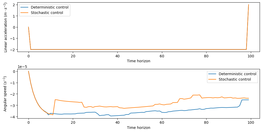
Figure 1: Control values for an example scenario.

4.1 Shortcomings of the deterministic model

The deterministic model presents bad performances compared to the stochastic model and is subject to a high risk of collision in discrete time [1], modelled as the number of times the constraint g is violated per realisation of a scenario (experiment 1) or per scenario (experiment 2). To show the robustness of the stochastic model, the following Figure 2 presents the number of violations for the deterministic models in continuous-time and discrete-time, with a corpus of 200 driving scenarios with different levels of risk.

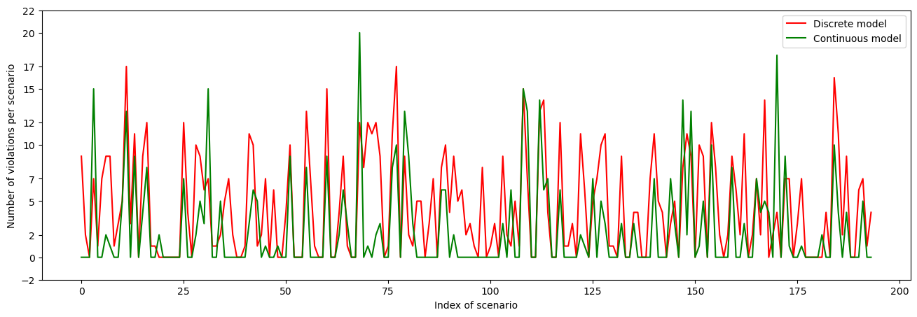
Figure 2: Violations of constraints for deterministic models in discrete-time and continuous-time.

The number of violations of the constraint is very high for both models. We can conclude that the deterministic model is not robust enough for our optimal control problem and should not be favoured over stochastic models. In the remainder of this study, we conduct our experiments for stochastic models only.

4.2 Convergence speed of continuous-time solving

$\mathbf{w}_{g}:\mathbf{w}_{v}:\mathbf{w}_{a}:\mathbf{w}_{\omega}:\mathbf{w}_{j}:\mathbf{w}_{h}:\mathbf{w}_{p}$		5:1:1:1:1:1:1			1:5:1:1:1:1:1
$T$		50	200	400	50	200	400
Average CPU times		0.261	0.800	1.079	0.322	0.794	1.035
Average acceleration		1.961	1.98	1.532	1.849	1.732	1.373
Average angular velocity		0	0	0	0	0	0
Average velocity		14.743	15.741	17.031	14.718	15.667	16.861
Average distance		14.764	31.523	68.265	14.739	31.375	67.589
$\mathbf{w}_{g}:\mathbf{w}_{v}:\mathbf{w}_{a}:\mathbf{w}_{\omega}:\mathbf{w}_{j}:\mathbf{w}_{h}:\mathbf{w}_{p}$		1:1:5:1:1:1:1			1:1:1:5:1:1:1
$T$		50	200	400	50	200	400
Average CPU times		0.247	0.744	1.145	0.251	0.804	1.045
Average acceleration		1.960	1.972	1.437	1.960	1.928	1.436
Average angular velocity		0	0	0	0	0	0
Average velocity		14.743	15.730	17.029	14.743	15.727	17.019
Average distance		14.764	31.501	68.256	14.764	31.496	68.220
$\mathbf{w}_{g}:\mathbf{w}_{v}:\mathbf{w}_{a}:\mathbf{w}_{\omega}:\mathbf{w}_{j}:\mathbf{w}_{h}:\mathbf{w}_{p}$		1:1:1:1:5:1:1			1:1:1:1:1:5:1
$T$		50	200	400	50	200	400
Average CPU times		0.245	0.795	1.044	0.249	0.947	1.060
Average acceleration		1.961	1.928	1.436	1.960	1.928	1.436
Average angular velocity		0	0	0	0	0	0
Average velocity		14.743	15.727	17.019	14.743	15.727	17.019
Average distance		14.764	31.496	68.220	14.739	31.375	68.220
$\mathbf{w}_{g}:\mathbf{w}_{v}:\mathbf{w}_{a}:\mathbf{w}_{\omega}:\mathbf{w}_{j}:\mathbf{w}_{h}:\mathbf{w}_{p}$		1:1:1:1:1:1:5			1:1:1:1:1:1:1
$T$		50	200	400	50	200	400
Average CPU times		0.242	0.799	1.038	0.241	0.797	1.043
Average acceleration		1.960	1.928	1.436	1.960	1.928	1.436
Average angular velocity		0	0	0	0	0	0
Average velocity		14.743	15.727	17.019	14.743	15.727	17.019
Average distance		14.764	31.496	68.220	14.739	31.375	68.220

Table 2: Comparison under different configurations over 100 different scenarios of the continuous-time model.

Other input parameters have to be designed; they are the weights $(\mathbf{w}_{g},\mathbf{w}_{v},\mathbf{w}_{a},\mathbf{w}_{\omega},\mathbf{w}_{j},\mathbf{w}_{h},\mathbf{w}_{p})$.

Table 2 shows analytics for different configurations of those weights. As in [1], the sensors are imperfect, and their measures contain errors which are modelled by adding a random noise with a normal distribution $\mathcal{N}(0,1)$ over the real positions of the target vehicle. To compare the analytics of our model with the different configurations without considering the effects of the random noises, we look at the average of control-state values over a sample of 100 different scenarios for each set of weights.

The time horizons $T$ considered here have higher values than the number of samples $N$ for discrete-time analysis [1], thanks to dynamic solvers in continuous time which can handle far horizons. Steady-state real-time optimisation used in GEKKO [16] for discrete-time optimal control problems requires solving $N$ different control-state equations, as each variable describes a time-step $k$. In contrast, dynamic solvers solve the equation for each control-state variable through the time horizon. In addition, the average CPU times are lower than for the discrete-time model [1]. The dynamics are similar for each set of weights, as they increase proportionally with the time horizons. The most significant increases in computational time are for weights $\mathbf{w}_{a}$ and $\mathbf{w}_{v}$. However, the continuous-time model is still faster and goes beyond the limits of the discrete-time model, as we develop in Section 4.6

4.3 Experiment 1: one risky scenario

The scenario introduced for our first experiment presents the trajectory illustrated in Figure 3 : :

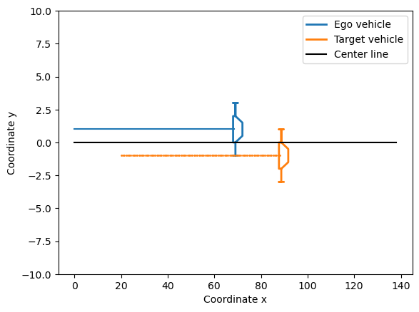
Figure 3: Trajectory of ego and target vehicles.

In the risky scenario, the input parameter which changes from the classic urban driving scenario as described in Table 1 is the recommended linear speed $v_{r}$, from a value of $12\ m.s^{-1}$ representing the average speed of vehicles in cities to a value of $14\ m.s^{-1}$ which is a little bit above the maximum speed limit of $50\ km.h^{-1}$ in urban areas.

This first experiment focuses on assessing the robustness of our continuous model, that is, its capacity to give a solution for the trajectory planning problem even with uncertainties in measured data. Here, we suppose $(x^{tgt}_{t},x^{tgt}_{t})_{t\in[0,T]}$ to be sampled from random variables as in (4) and (5), and we perform 200 realisations.

The number of steps for the discrete-time model and the time horizon for the continuous-time model are fixed with lower values for the first experiment than in the second experiment, where the scenarios are considered well-dimensioned. If they are not dimensioned correctly, the optimal control problem for trajectory planning does not guarantee convergence to a feasible or realistic solution. As an example, if the linear recommended speed $v_{r}$ is too high and the associated weight $\mathbf{w}_{v}$ is large enough, the solution of the optimal control problem could give the ego vehicle to remain motionless at the beginning and wait for some time before accelerating. The horizon is lower to prevent this phenomenon in the simulation, especially in risky scenarios. When the speed increases, other parameters must be adapted to dimension different scenarios, as we do in Section 4.6 to model road and highway driving scenarios.

Figure 4 shows the value of the quantity $d_{min}-K(x^{tgt}_{t},y^{tgt}_{t},x_{t},y_{t})$ derived from constraint (g) for each realisation, on the time interval $[0;T]$ for the continuous model and on the steps $\{1,...,N\}$ for the discrete model. We show both zoomed-in and entire visualisations for both stochastic models. A constraint violation is visualised on positive values, which implies $d_{min}>K(x^{tgt}_{t},y^{tgt}_{t},x_{t},y_{t})$ for a given time $t$. For this specific time $t$, the vehicles are too close to what we would have expected based on the constraints defined in our model.

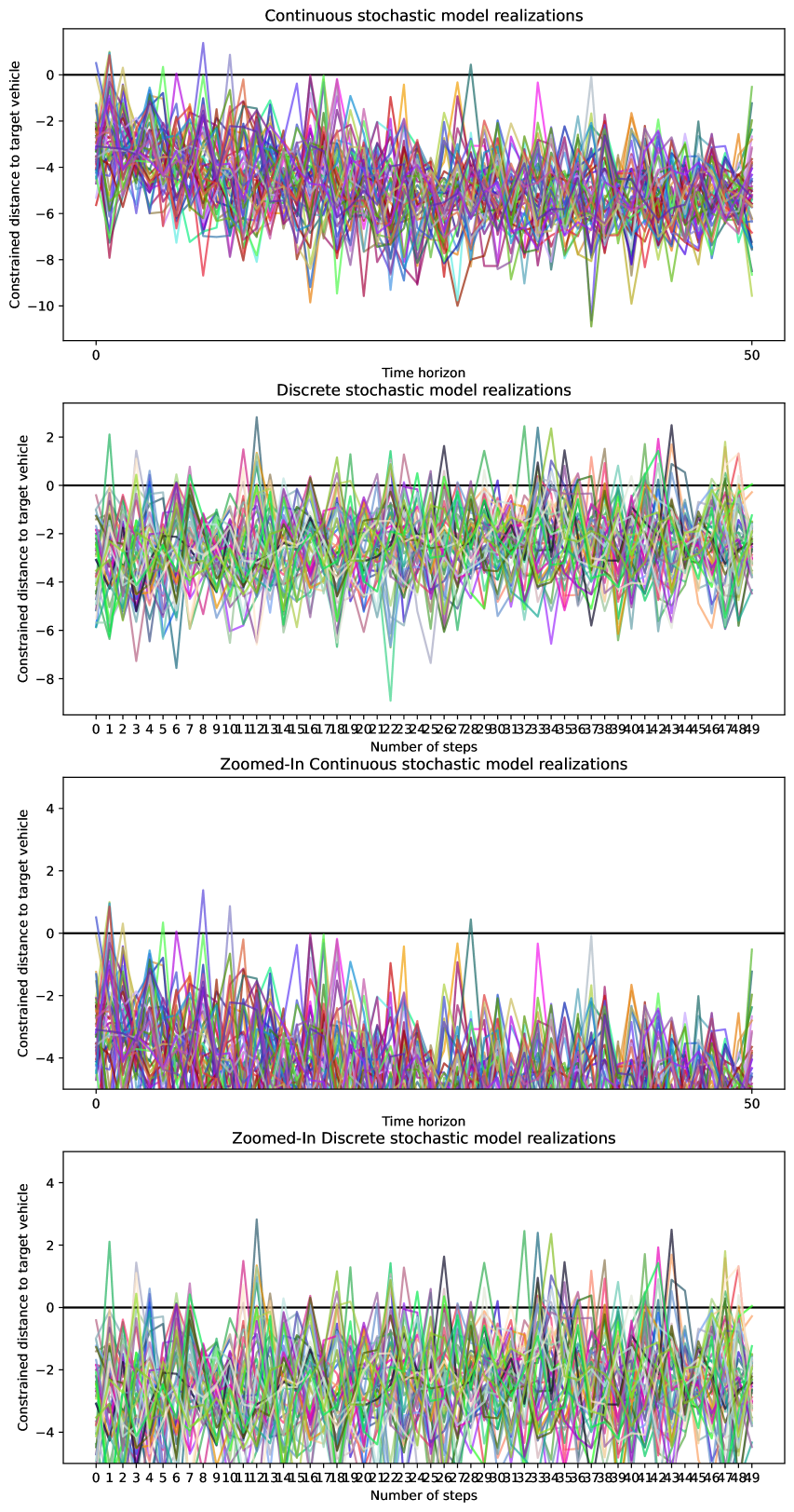
Figure 4: Constraint function values of all realisations of the scenario for stochastic models.

Figure 5 represents the number of violations for each realisation for stochastic models in discrete-time and continuous-time frameworks. As the scenario considered here has been chosen as risky, we have more constraint violations in the realisations than for unstressed urban driving scenarios, as discussed in the second experiment Section 4.4. However, the discrete-time model reaches the highest number of violations, and the average number of violations per realisation is higher for the discrete-time stochastic model than the continuous-time stochastic model. Figure 6 presents the histogram of the number of realisations per number of violations, and most realisations have less than one violation for continuous-time while a large part of discrete-time realisations has more than two violations.

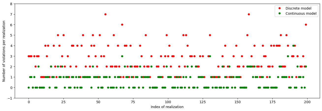
Figure 5: Number of violations per realisation of the scenario for stochastic models.

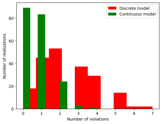
Figure 6: Histogram of the number of violations per realisation of the scenario for stochastic models.

4.4 Experiment 2: multiple scenarios

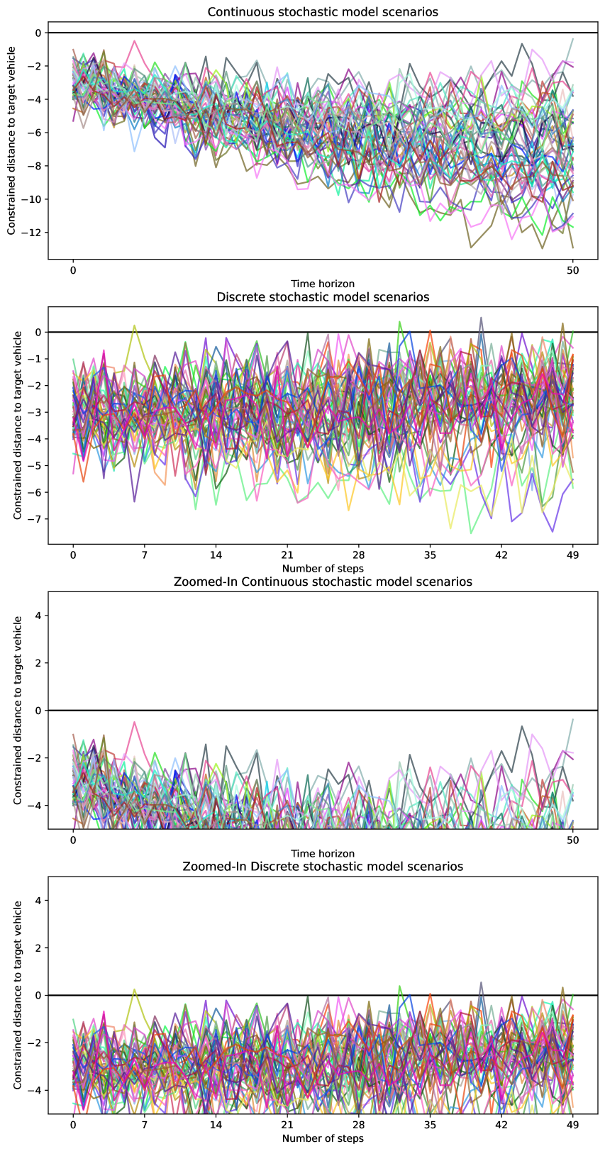
Figure 7: Constraint function values of all scenarios for stochastic models.

As in the previous experiment, Figure 7 visualises the value of the quantity $d_{min}-K(x^{tgt}_{t},y^{tgt}_{t},x_{t},y_{t})$ through time, for each simulated scenario. Violations are the positive values of the curves. Those scenarios are various urban driving scenarios generated from the simulator. As those are less risky scenarios than in the first experiment, both stochastic models perform better.

Figure 8 and 9 are, respectively, the representations of the number of violations per scenario and histograms of the number of scenarios per number of violations, as we visualised for each realisation in Section 4.3. Observations show that in over 200 scenarios, the number of violations is meagre. The discrete-time stochastic model presents at most two violations and the continuous-time stochastic model presents at most one violation in a few scenarios. The histogram shows no violations for more than 180 scenarios for the continuous-time model and more than 150 scenarios for the discrete-time one. The continuous-time model also performs best in this experiment compared to the discrete-time model, but the stochastic approach in both cases guarantees good results.

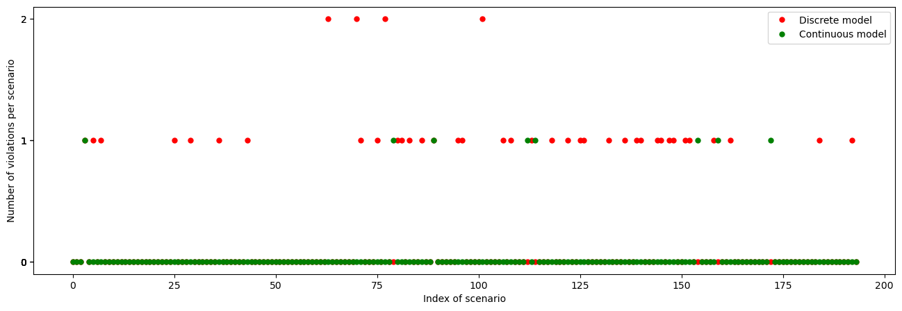
Figure 8: Number of violations per scenario for stochastic models.

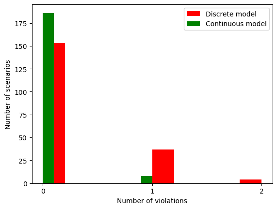
Figure 9: Histogram of the number of violations per realisation of the scenario for stochastic models.

4.5 Chance-constraints in stochastic models

Figure 10 is a representation of the chance constraint (6) over all scenarios for both discrete-time and continuous-time models. We have chosen a confidence value $\alpha=0.95$, represented as a bold line on this figure. The stochastic constraints (4) and (5) are sufficiently robust to guarantee the ego vehicle does not violate the constraint $95\%$ of the time through one simulation. The continuous-time stochastic model performs better than the discrete-time stochastic model, as for 200 scenarios, the model is valid more than $99\%$ of the time.

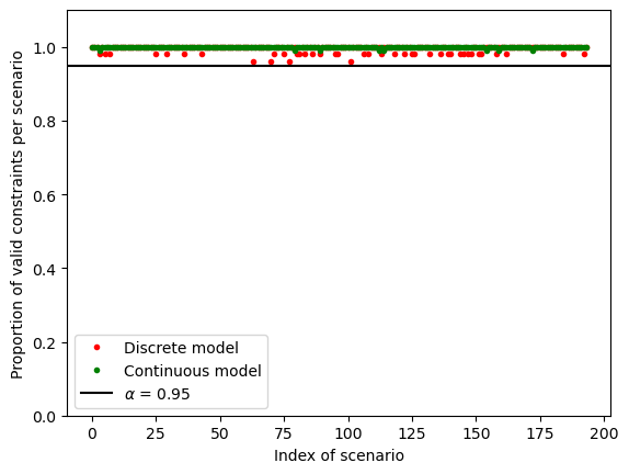
Figure 10: Proportion of valid constraints per scenario for discrete-time and continuous-time stochastic models

4.6 Robustness of continuous-time model to high time horizons $T$

The continuous model performs better than the discrete model, but both provide satisfactory results, thanks to the stochastic approach.

The advantage of the continuous-time model is to handle a large time horizon ($T>=100$) where the discrete model presents limitations over the number of steps $N$. Therefore, the continuous model can handle scenarios other than those studied in Section 4.3 and Section 4.4, allowing higher speeds (driving on roads outside city restrictions, highways). For safety reasons, we need to perform trajectory planning over far horizons when the speed increases. This approach requires more data points but is more robust to prevent unexpected events and have a precautionary approach to driving.

	Continuous model			Discrete model
$v_{r}/\omega_{max}$	$\frac{\pi}{6}$	$\frac{\pi}{4}$	$\frac{\pi}{2}$	$\frac{\pi}{6}$	$\frac{\pi}{4}$	$\frac{\pi}{2}$
$22\ m.s^{-1}$	$96$	$98$	$99$	$6$	$7$	$2$
$36\ m.s^{-1}$	$85$	$95$	$92$	$3$	$4$	$1$

Table 3: Number of solutions found over 100 scenarios.

Table 3 presents the number of solutions found for 100 scenarios, given different constraints over the control.
For this experiment, the computation time is $\approx 30$ minutes for the discrete-time model and $\approx 5$ minutes for the continuous-time one.

The discrete-time model does not find a solution for all real-life scenarios, as the driving is continuous, so some information about the environment can be lost when discretising. The solver is robust enough to find feasible solutions in continuous time when the scenarios are more diverse concerning target vehicle speed and centre lane variations.

5 Conclusions and Future Work

This paper shows the effectiveness of a continuous-time approach for optimal control-based reference trajectory generation compared to a discrete-time framework. Chance-constrained optimisation addresses the stochastic aspect of the model, which considers the uncertainty of information concerning autonomous vehicles. Our analysis showed low performance for deterministic models compared to the stochastic models in continuous-time. Good results are obtained for urban driving scenarios with both continuous-time and discrete-time stochastic models, with slightly better results in continuous-time, specifically for risky scenarios where it diminishes the risks of collisions. Still, the discrete-time stochastic model fails to find solutions for roads and highways with higher speed limits, as those scenarios require planning over far time horizons. The computation time is higher for the discrete-time stochastic model as the number of control-state variables increases with the horizon. The continuous-time stochastic model reflects real-life driving conditions better and converges faster to an optimal solution.

Further work would consider enhancements to the vehicle model to tackle other aspects of road conditions, with more vehicles considered in the planning. Dealing with the uncertainty of information on the environment is a tough challenge in modelling autonomous vehicles, so another extension could be to consider new terms in the objective function and constraints over our stochastic optimal control problem.

References

- [1] Shangyuan Zhang, Makhlouf Hadji, and Abdel Lisser. Optimal control based trajectory planning under uncertainty. In International Conference on Intelligent Transport Systems, pages 73–88. Springer, 2022.
- [2] Sterling J Anderson, Steven C Peters, Tom E Pilutti, and Karl Iagnemma. An optimal-control-based framework for trajectory planning, threat assessment, and semi-autonomous control of passenger vehicles in hazard avoidance scenarios. International Journal of Vehicle Autonomous Systems, 8(2-4):190–216, 2010.
- [3] Deok-Kee Choi. Motion tracking of four-wheeled mobile robots in outdoor environments using bayes’ filters. International Journal of Precision Engineering and Manufacturing, 24(5):767–786, 2023.
- [4] Rafał M Sobański, Maciej M Michałek, and Michael Defoort. Predefined-time vfo control design for unicycle-like mobile robots. Nonlinear Dynamics, 112(5):3591–3603, 2024.
- [5] Dieky Adzkiya, Muhammad Syifa’ul Mufid, Febrianti Silviana Saputri, and Alessandro Abate. Control design of discrete-time unicycle model using satisfiability modulo theory. Systems Science & Control Engineering, 12(1):2316166, 2024.
- [6] Loïck Degorre, Emmanuel Delaleau, and Olivier Chocron. A survey on model-based control and guidance principles for autonomous marine vehicles. Journal of Marine Science and Engineering, 11(2):430, 2023.
- [7] Chalavadi Vishnu, Vineel Abhinav, Debaditya Roy, C Krishna Mohan, and Ch Sobhan Babu. Improving multi-agent trajectory prediction using traffic states on interactive driving scenarios. IEEE Robotics and Automation Letters, 8(5):2708–2715, 2023.
- [8] Qingzhao Zhang, Shengtuo Hu, Jiachen Sun, Qi Alfred Chen, and Z Morley Mao. On adversarial robustness of trajectory prediction for autonomous vehicles. In Proceedings of the IEEE/CVF Conference on Computer Vision and Pattern Recognition, pages 15159–15168, 2022.
- [9] Kai Ren, Heejin Ahn, and Maryam Kamgarpour. Chance-constrained trajectory planning with multimodal environmental uncertainty. IEEE Control Systems Letters, 7:13–18, 2022.
- [10] Sean Vaskov, Rien Quirynen, Marcel Menner, and Karl Berntorp. Friction-adaptive stochastic nonlinear model predictive control for autonomous vehicles. Vehicle System Dynamics, 62(2):347–371, 2024.
- [11] Allen Wang, Ashkan Jasour, and Brian C Williams. Non-gaussian chance-constrained trajectory planning for autonomous vehicles under agent uncertainty. IEEE Robotics and Automation Letters, 5(4):6041–6048, 2020.
- [12] Wilko Schwarting, Javier Alonso-Mora, and Daniela Rus. Planning and decision-making for autonomous vehicles. Annual Review of Control, Robotics, and Autonomous Systems, 1:187–210, 2018.
- [13] Lienhung Chen, Zhongliang Jiang, Long Cheng, Alois C Knoll, and Mingchuan Zhou. Deep reinforcement learning based trajectory planning under uncertain constraints. Frontiers in Neurorobotics, 16:883562, 2022.
- [14] Edgar N Sanchez and Fernando Ornelas-Tellez. Discrete-time inverse optimal control for nonlinear systems. CRC Press, 2017.
- [15] Chang Liu, Seungho Lee, Scott Varnhagen, and H Eric Tseng. Path planning for autonomous vehicles using model predictive control. In 2017 IEEE Intelligent Vehicles Symposium (IV), pages 174–179. IEEE, 2017.
- [16] Logan Beal, Daniel Hill, R Martin, and John Hedengren. Gekko optimization suite. Processes, 6(8):106, 2018.
- [17] James Blake Rawlings, David Q Mayne, and Moritz Diehl. Model predictive control: theory, computation, and design, volume 2. Nob Hill Publishing Madison, WI, 2017.
- [18] Thomas Nguen That and Jordi Casas. An integrated framework combining a traffic simulator and a driving simulator. Procedia-Social and Behavioral Sciences, 20:648–655, 2011.