Superconductivity from spin-canting fluctuations in rhombohedral graphene

Abstract

Rhombohedral graphene multilayers host various broken-symmetry metallic phases as well as superconductors whose pairing mechanism and order parameter symmetry remain unsettled. Strikingly, experiments have revealed prominent new superconducting regions in rhombohedral bilayer and trilayer graphene devices with proximity-induced Ising spin-orbit coupling. We propose that these superconductors descend from a common spin-canted normal state that spontaneously breaks a U(1) spin symmetry and thus supports a gapless (Goldstone) magnon mode. In particular, we develop a scenario wherein pairing in the spin-canted state emerges from a novel type of magnon-mediated attraction: Contrary to conventional mechanisms that involve the exchange of a single boson, we show that second-order processes that exchange two magnons are dominant and produce an $s$-wave pairing interaction featuring a unique logarithmic low-frequency divergence. This low-frequency divergence disappears when spin-orbit coupling vanishes, providing a promising explanation for spin-orbit-enabled pairing. Numerous other experimental observations—including nontrivial dependence of superconductivity on the spin-orbit coupling strength, in-plane magnetic fields, and Fermi surface structure—also naturally follow from our scenario.

I Introduction

Rhombohedral graphene—composed of layers stacked in an ‘ABC’ pattern—provides an extremely clean, gate-tunable platform for emergent quantum phenomena [1, 2, 3, 4, 5, 6, 7, 8, 9, 10, 11]. As prominent examples, ‘pure’ bilayer and trilayer devices (i.e., without proximity effects from adjacent 2D materials) exhibit exceptionally rich phase diagrams. Indeed, electrically varying the density and perpendicular displacement field reveals a series of correlated metallic states as well as unconventional superconductors [4, 5, 6, 7]. Despite detailed distinctions such as fermiology, normal-state order, and response to magnetic fields, these superconducting states share a common unifying ingredient: Each one appears tethered to a narrow density window close to a normal-state phase transition, prompting the investigation of pairing scenarios based on critical fluctuations [12, 13, 14, 15] and other mechanisms [16, 17, 18, 19, 20, 21, 22, 23, 24, 25, 26, 27, 28].

Placing rhombohedral bilayers and trilayers proximate to a transition metal dichalcogenide (TMD) effectively boosts graphene’s spin-orbit coupling by orders of magnitude [29, 30, 31, 32, 33, 34, 35, 36, 37, 38, 39, 40, 41, 42, 43], in turn enriching the phenomenology in a very interesting way. Namely, new superconducting phases emerge that display the following salient features [36, 37, 40, 39, 38, 41]: $(i)$ Rather than residing near a phase boundary, they occur over a broad density range within a normal state that hosts two large majority Fermi pockets coexisting with some number of small minority pockets. $(ii)$ Their optimal critical temperatures $T_{c}$ far exceed those arising in ‘pure’ devices. And $(iii)$ their susceptibility to depairing by in-plane magnetic fields varies nontrivially across the superconducting regions. Numerous scenarios for how spin-orbit coupling promotes Cooper pairing in this setting have been introduced [36, 44, 45, 26, 27, 46, 47, 28]. Subsequent experiments on bilayers [38] further showed that, as the spin-orbit-coupling imparted by the TMD increases, the strongest new superconductor populates a diminished area in the phase diagram—yet curiously exhibits an enhanced maximal $T_{c}$.

Our goal here is to develop a unified scenario that accounts for these characteristics of (ostensibly) spin-orbit-enabled superconductors in both bilayers and trilayers. More specifically, we will address the following questions: What is the appropriate normal state that gives way to superconductivity? What is the pairing mechanism, and how is it ‘activated’ by spin-orbit coupling? Given a putative normal state and pairing mechanism, how can one recover the detailed phenomenology highlighted above (which places stringent constraints on theory)?

It is instructive to first address the fate of the normal state in ‘pure’ bilayer and trilayer devices without an adjacent TMD, where to a good approximation the system preserves SU(2) spin-rotation symmetry. In the relevant density and displacement field regime, quantum oscillation measurements clearly evidence lifting of graphene’s spin/valley degeneracy by interactions, yielding a broken-symmetry metallic state with majority and minority carriers. We will assume that this phase corresponds to a simple Stoner ferromagnet that spontaneously breaks the SU(2) symmetry by developing an arbitrarily oriented spin magnetization. This assumption is bolstered by experiments (specifically, magnetic field dependence of the phase boundary with adjacent symmetric and/or spin-and-valley polarized states, as well as a vanishing anomalous Hall signal [3, 5]). Moreover, Hartree-Fock simulations find that this order is stabilized by long-range Coulomb repulsion supplemented by ferromagnetic Hund’s coupling $J$ that favors aligning the spins in the $K$ and $K^{\prime}$ valleys [3, 20, 12, 48, 49].

Anchored by this plausible ansatz, we then ask how the Stoner ferromagnet evolves upon resurrecting spin-orbit interaction inherited from the TMD. Throughout this work we assume that the TMD primarily engenders Ising spin-orbit coupling $\lambda_{I}$, which preserves a U(1) subgroup of SU(2) corresponding to spin rotations about an out-of-plane Ising axis. By itself, $\lambda_{I}$ favors orienting the spins normal to the graphene layers, in opposite directions for the two valleys—clearly competing with the different spin profile favored by Hund’s coupling. As demonstrated by Hartree-Fock simulations [48], over a finite window of $\lambda_{I}$ the system can reach a compromise by realizing a spin-canted phase: Here, the spins tilt away from the Ising axis by a canting angle $\theta_{0}$ as shown in Fig. 1, spontaneously breaking the U(1) symmetry by developing an in-plane spin magnetization that partially satisfies $J$. This logic leads us to postulate that the normal state for spin-orbit-enabled superconductors in both bilayers and trilayers hosts spin-canting order.

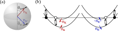
Figure 1: Summary of the proposed pairing mechanism. (a) Illustration of spin-canting order. The spin polarization ${\boldsymbol{n}}_{K}$ (${\boldsymbol{n}}_{K^{\prime}}$) in each valley is represented by a red (blue) arrow on the Bloch sphere. Ising spin-orbit interaction defines an out-of-plane quantization axis that points in opposite directions in the two valleys. Spin-canted order arises when an in-plane magnetic moment is spontaneously generated, leading to a non-trivial polar angle $\theta_{0}$ of the magnetization vectors and an arbitrarily-chosen azimuthal angle. Gapless magnon (Goldstone) modes associated with the spontaneous symmetry breaking are shown by black arrows. (b) The gapless magnons can mediate pairing in each Fermi surface through a second-order process that scatters Cooper pairs to the other band and back. This interaction yields an $s$-wave order parameter and is divergent at low frequencies, providing crucial retardation effects that benefit superconductivity.

Given that the spin-canted phase evolves smoothly from a simple Stoner ferromagnet upon turning on $\lambda_{I}$, one can then ask why the former would be more conducive to Cooper pairing than the latter. A first hint surfaces from examining their collective modes. Both phases spontaneously break a continuous symmetry—U(1) spin rotations for the spin-canted phase and SU(2) for the Stoner ferromagnet—and hence both support gapless Goldstone magnon excitations. A qualitative distinction nevertheless exists: Because of the preceding symmetry distinction, the Goldstone mode disperses linearly with momentum for the spin-canted phase but quadratically with momentum for the Stoner ferromagnet. Might then low-energy magnon modes provide a pairing glue whose effectiveness depends critically on their dispersion?

We show that linearly dispersing magnons in the spin-canted phase can efficiently mediate attraction via a novel mechanism that differs sharply from conventional boson-mediated pairing. In the conventional picture, superconductivity emerges from Cooper pairs scattering via the exchange of a single boson (most commonly a phonon). Due to kinematic constraints, however, exchange of single low-energy magnons is ineffective at mediating pairing in the spin-canted phase. Nevertheless, we find that two-magnon exchange processes—wherein Cooper pairs near the Fermi surface scatter to virtual high-energy states and then back—gives rise to a pairing interaction that diverges at low frequency and favors $s$-wave superconductivity. This divergence encodes strong attraction over a narrow frequency range, implying significant retardation effects that are crucial for overcoming the pair-breaking tendencies of Coulomb repulsion. Interestingly, strong pairing arises here because two-magnon processes provide a way around a well-known constraint on the coupling strength between Goldstone modes and electrons [50] (see discussion in Sec. III.1). We additionally establish that two-magnon exchange events dominate over all higher-magnon processes, and that self-energy corrections do not spoil the pairing instability. Crucially, in the absence of spin orbital coupling, quadratically dispersing magnons characteristic of the simple SU(2) Stoner ferromagnet yield only a non-divergent pairing interaction. Two-magnon exchange operating within a spin-canted phase therefore naturally accounts for spin-orbit-enabled superconductivity in rhombohedral graphene.

Our proposed scenario also accommodates more refined experimerimental observations enumerated earlier. First, recall that spin-orbit-enabled superconductivity entails small minority Fermi pockets; moreover, in trilayers superconductivity abruptly turns off when they are vacated through a Lifshitz transition [40]. These observations hint that pairing may originate primarily from minority carriers. We predict that, due to the divergent nature of the magnon-mediated pairing interaction, its strength within a given Fermi surface scales inversely with the corresponding Fermi momentum—hence pairing indeed preferentially arises in small pockets.

Second, Ref. 38 observed a tunable and gradual increase of the maximal $T_{c}$ with induced Ising spin-orbit-coupling $\lambda_{I}$, coinciding with a counter-intuitive reduction in the phase space occupied by superconductivity. Our scenario recovers these seemingly at odds trends as follows. The gradual rise in achievable $T_{c}$ simply reflects the fact that spin-orbit coupling is crucial for producing a divergent, narrow-band pairing interaction as already noted. We find that the pairing interaction depends sensitively on the canting angle $\theta_{0}$ and scales roughly linearly with $\lambda_{I}$; see Fig. 2. Ising spin-orbit interaction simultaneously competes, however, against Hund’s coupling that is responsible for in-plane ferromagnetism and the associated Goldstone mode [3, 5]. Consequently, increasing $\lambda_{I}$ chips away at the phase space occupied by the spin-canting phase—as seen in Hartree-Fock simulations [48]—and in doing so shrinks the parameter regime in which the magnon-mediated pairing glue thrives.

Our theory may also explain unusual trends seen in the effects of in-plane magnetic fields on spin-orbit-enabled superconductivity. While naively one might anticipate high tolerance to in-plane magnetic fields due to Ising spin-orbit interaction [51, 52], experiments have measured critical in-plane fields that vary from well above the Pauli limit to below the Pauli limit depending on parameters [36, 37, 39, 40, 38]. Orbital or Rashba spin-orbit effects may at least partially explain these trends, though our scenario predicts a new depairing mechanism that could dominate the in-plane field response. Specifically, in-plane magnetic fields explicitly break the U(1) spin symmetry that the spin-canting phase breaks spontaneously—thereby gapping out the Goldstone mode, cutting off the low-frequency divergence in the pairing interaction, and sharply reducing the effectiveness of magnon-mediated pairing. This behavior stands in stark contrast to non-magnetic pairing glues, such as phonons, where superconductivity would be suppressed primarily by field-induced breaking of pairing resonances at the Fermi energy.

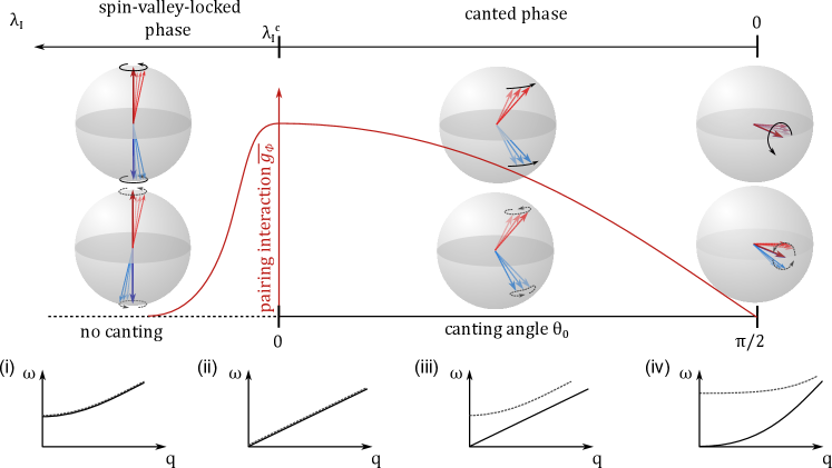
Figure 2: Magnon modes and pairing interaction. The upper line illustrates the presumed phase diagram as a function of Ising spin-orbit coupling $\lambda_{I}$; a spin-canted phase appears up to a critical value $\lambda_{I}^{c}$, beyond which a symmetric spin-valley-locked phase emerges. The red curve sketches the magnon-mediated pairing interaction strength [see Eq. (50)], which depends sensitively on the canting angle $\theta_{0}$ and hence on spin-orbit coupling. Spheres illustrate the two relevant magnon modes in each regime: a valley-symmetric mode ($s-$, solid black arrow) and a valley-antisymmetric mode ($a-$, dashed gray arrow)—in valleys $K$ (blue arrows) and $K^{\prime}$ (red arrows). Insets (i)-(iv) show the associated magnon spectra. (i) In the symmetric spin-valley-locked phase, both magnon modes are gapped, and the pairing interaction is correspondingly suppressed. (ii) At the spin-canting phase transition both modes become gapless and have identical low-energy dispersion, and both contribute non-negligibly to the pairing interaction. (iii) In the canted phase where $\theta_{0}\neq 0$, the only gapless mode is the Goldstone mode $s-$ associated with the spontaneous symmetry breaking. (iv) When $\theta_{0}\rightarrow\pi/2$ (corresponding to vanishing spin-orbit interaction), the $s-$ mode acquires quadratic dispersion characteristic of an SU(2) ferromagnet. In this limit we show that the magnon-mediated pairing interaction is qualitatively suppressed.

We organize the rest of this article as follows. Section II describes the phenomenology of the spin-canted phase in rhombohedral graphene, using both an effective Landau-theory description as well as a microscopic model from which we extract the magnon spectrum. Section III derives the form of magnon-mediated interactions between electrons, and Sec. IV then investigates the Cooper-pairing problem mediated by those interactions. Section V addresses the survival of pairing when incorporating self-energy corrections. Finally, Sec. VI compares our predictions to prior experimental observations and proposes several future directions.

II Phenomenology of the spin-canted phase

In this section we present the phenomenology of the spin-canted phase that forms the basis of our proposed mechanism for spin-orbit-enabled superconductivity in rhombohedral graphene. We capture this symmetry-breaking order from both Landau theory and a physically motivated microscopic model; additionally, we will use the latter to study the magnon spectrum.

II.1 Landau-theory description

Many of the symmetry-breaking metallic phases observed in rhombohedral graphene can be understood within the generalized Stoner ferromagnetism picture, whereby a subset of the four spin and valley flavors are preferentially occupied. Here we focus on the situation in which symmetry-breaking order can be captured by the spin polarization ${\boldsymbol{n}}_{\xi}$ in valley $\xi=K,K^{\prime}$. The magnitude $n_{\xi}$ is essentially the density difference between the majority and minority spin flavors in valley $\xi$, while the direction $\hat{{\boldsymbol{n}}}_{\xi}$ sets the spin orientations for the majority and minority carriers. Throughout this section we assume that all order parameters are uniform in real-space (i.e., we only consider their ${\boldsymbol{q}}=0$ components).

A minimal free energy density describing generalized Stoner ferromagnetism in spin-orbit-proximitized devices reads [3]

$${\cal F}=\frac{\kappa_{s}}{2}\sum_{\xi}{\boldsymbol{n}}_{\xi}^{2}-J{\boldsymbol{n}}_{K}\cdot{\boldsymbol{n}}_{K^{\prime}}+\frac{\lambda_{I}}{2}\sum_{\xi}\tau_{\xi}n^{z}_{\xi}+\cdots.$$ (1)

In the first term—which is invariant under independent SU(2) spin rotations in the two valleys—$\kappa_{s}$ encodes a combination of intravalley exchange interactions and kinetic energy. Near the onset of a Stoner transition driven primarily by these ingredients, $\kappa_{s}$ turns negative and promotes the development of non-zero order parameters ${\boldsymbol{n}}_{\xi}$. Intervalley exchange processes are modeled by the second term, which breaks the symmetry of the $\kappa_{s}$ term down to global SU(2) spin rotations. We assume $J>0$, corresponding to ferromagnetic Hund’s coupling that favors aligning spins for the two valleys. In the third term, $\tau_{K,K^{\prime}}=\pm 1$ is a valley-dependent sign and $\lambda_{I}$ denotes Ising spin-orbit coupling that favors spins pointing out-of-plane, in opposite directions in the two valleys, denoted as $\pm\hat{\bf z}$. Ising spin-orbit coupling further reduces the symmetry down to global U(1) spin rotations around the $z$ axis. For concreteness, we assume $\lambda_{I}\geq 0$ throughout. Finally, the ellipsis denotes symmetry-allowed that are higher-order in ${\boldsymbol{n}}_{\xi}$ (e.g., cubic and quartic terms). Such terms fix the order-parameter magnitudes in the ordered phase and also determine whether the Stoner transition is continuous or first-order [53]. Importantly, our analysis applies regardless of the order of the phase transition.

Let us denote the vectors ${\boldsymbol{n}}_{\xi}$ by their magnitudes $n_{\xi}$, their polar angles $\theta_{\xi}$ measured from the $+\hat{\bf z}$ direction, and their azimuthal angles $\phi_{\xi}$. The free energy is minimized when the azimuthal angles match, $\phi_{+}=\phi_{-}$, because such configurations optimize the $J$ term without penalizing the $\kappa_{s}$ or $\lambda_{I}$ contributions. We further consider solutions where the order-parameter amplitudes agree, $n_{K}=n_{K^{\prime}}\equiv n_{0}$. Competing orders with unequal $n_{K}$ and $n_{K^{\prime}}$ [49] can be excluded on phenomenological grounds due to their non-zero valley polarization, which is highly detrimental to zero-momentum pairing.

Imposing the preceding two restrictions yields a free energy density dependent only on $n_{0}$ and $\theta_{\xi}$:

$${\cal F}=\kappa_{s}n_{0}^{2}-Jn_{0}^{2}\cos(\theta_{+}-\theta_{-})+\frac{\lambda_{I}}{2}n_{0}\left(\cos\theta_{+}-\cos\theta_{-}\right)+\cdots$$ (2)

Next we observe that Eq. (2) is minimized—assuming $\lambda_{I}\neq 0$—by solutions of the form $\theta_{+}=\pi-\theta_{-}$ and $\theta_{-}\equiv\theta_{0}$. Specializing to such configurations yields

$${\cal F}=\kappa_{s}n_{0}^{2}+Jn_{0}^{2}\cos 2\theta_{0}-\lambda_{I}n_{0}\cos\theta_{0}+\cdots,$$ (3)

which admits two types of ordered states with $n_{0}\neq 0$: $(i)$ For $\lambda_{I}>4Jn_{0}$, the system minimizes its free energy by selecting $\theta_{0}=0$, corresponding to an Ising spin-valley-locked phase that preserves U(1) spin rotation symmetry. $(ii)$ For $\lambda_{I}<4Jn_{0}$, a spin-canted phase emerges with canting angle

$$\theta_{0}=\arccos\left({\frac{\lambda_{I}}{4Jn_{0}}}\right)$$ (4)

that smoothly increases from 0 towards $\pi/2$ as $\lambda_{I}$ decreases. This phase crucially does spontaneously break the continuous U(1) spin-rotation symmetry due to the arbitrary orientation of the in-plane moment that develops from canting (see also Fig. 1), and correspondingly supports a linearly dispersing Goldstone mode.

For a rough order-of-magnitude estimate, suppose that $\lambda_{I}\sim 1$ meV and $J\sim 200$ meV nm² [3, 15, 25, 47, 49, 48]. With these parameters our free-energy analysis predicts that spin-canting order sets in when the density difference between majority and minority carriers exceeds $n_{0}^{c}\sim 10^{11}$ cm^-2. In proximitized rhombohedral bilayers [36, 37, 39, 38] and trilayers [40, 41], the normal state hosting the strongest superconductor exhibits polarization densities comparable to $n_{0}^{c}$, suggesting spin-canting order as a natural parent phase in agreement with Hartree-Fock simulations [48].

It is also instructive to consider the SU(2)-invariant limit with $\lambda_{I}=0$. Here the free energy in Eq. (1) is minimized in the ordered phase for any choice of the polar and azimuthal angles characterizing ${\boldsymbol{n}}_{\xi}$, provided they are identical for the two valleys. This phase spontaneously breaks SU(2) symmetry and also exhibits a Goldstone mode, albeit with quadratic rather than linear dispersion.

II.2 Microscopic model

For a more microscopic treatment, we now consider the Euclidean action

$$\mathcal{S}= \sum_{\xi}\int_{k}\overline{\psi}_{\xi,k}\left(-i\omega-\mu+\epsilon_{\xi,{\boldsymbol{k}}}-\frac{\lambda_{I}}{2}\tau_{\xi}\sigma^{z}\right)\psi_{\xi,k}$$

$$-\int_{q}\bigg{[}\frac{V}{2}\sum_{\xi}{\boldsymbol{s}}_{\xi}(q)\cdot{\boldsymbol{s}}_{\xi}(-q)+J{\boldsymbol{s}}_{K}(q)\cdot{\boldsymbol{s}}_{K^{\prime}}(-q)\bigg{]}.$$ (5)

In the sums $\xi=K,K^{\prime}$ is a valley index, while $k=(i\omega,{\boldsymbol{k}})$, $q=(i\nu,{\boldsymbol{q}})$ denote shorthand Matsubara frequencies and momenta. Here and below we use Pauli matrices $\sigma^{\alpha}$ that act in spin space and once again define $\tau_{K,K^{\prime}}=\pm 1$. (Spin indices are implicitly summed, though for clarity we explicitly display valley indices.) Grassman variables $\overline{\psi}_{\xi,k}$ and $\psi_{\xi,k}$ are associated with creation and annihilation operators, respectively, while ${\boldsymbol{s}}_{\xi}(q)=\int_{k}\overline{\psi}_{\xi,k+q}{\boldsymbol{\sigma}}\psi_{\xi,k}$ is the spin polarization operator for valley $\xi$. The first line of Eq. (5) encodes a chemical potential $\mu$ and spin-independent band energies $\epsilon_{\xi,{\boldsymbol{k}}}$ supplemented by Ising spin-orbit coupling $\lambda_{I}$. The second line incorporates phenomenological intravalley ($V>0$) and intervalley ($J>0$) ferromagnetic spin-spin interactions. In particular, the $V$ term, which is invariant under independent spin rotations in the two valleys, favors polarizing the spins separately in each valley, while $J$ represents a Hund’s coupling that favors aligning the spins in the two valleys. As in the free energy discussed in Sec. II.1, spin-canting order arises from the interplay between interaction parameters $V,J$ and the Ising coupling $\lambda_{I}$.

For convenience, we define the coupling matrix

$$g_{\xi\xi^{\prime}}=\left(\begin{matrix}V&J\\ J&V\end{matrix}\right)_{\xi\xi^{\prime}},$$ (6)

which allows us to more compactly express the action as

$$\mathcal{S} =\sum_{\xi}\int_{k}\overline{\psi}_{\xi,k}\left(-i\omega-\mu+\epsilon_{\xi,{\boldsymbol{k}}}-\frac{\lambda_{I}}{2}\tau_{\xi}\sigma^{z}\right)\psi_{\xi,k}$$

$$-\frac{1}{2}\sum_{\xi,\xi^{\prime}}\int_{q}g_{\xi\xi^{\prime}}{\boldsymbol{s}}_{\xi}(q)\cdot{\boldsymbol{s}}_{\xi^{\prime}}(-q).$$ (7)

Upon introducing an auxiliary field ${\boldsymbol{m}}_{\xi}(q)$, we may decouple the interactions via a Hubbard-Stratonovich transformation to arrive at

$$\mathcal{S} =\sum_{\xi}\int_{k}\overline{\psi}_{\xi,k}\left(-i\omega-\mu+\epsilon_{\xi,{\boldsymbol{k}}}-\frac{\lambda_{I}}{2}\tau_{\xi}\sigma^{z}\right)\psi_{\xi,k}$$

$$+\int_{q}\bigg{[}\frac{1}{2}\sum_{\xi,\xi^{\prime}}g^{-1}_{\xi\xi^{\prime}}{\boldsymbol{m}}_{\xi}(q)\cdot{\boldsymbol{m}}_{\xi^{\prime}}(-q)-\sum_{\xi}{\boldsymbol{m}}_{\xi}(q)\cdot{\boldsymbol{s}}_{\xi}(-q)\bigg{]}.$$ (8)

Next we explore the saddle points of the above action.

II.3 Saddle-point analysis

We specifically seek a uniform saddle-point solution and thus (for now) replace ${\boldsymbol{m}}_{\xi}(q)\rightarrow\delta(q)(-\frac{\lambda_{I}}{2}\tau_{\xi}{\bf\hat{z}}+\bar{{\boldsymbol{m}}}_{\xi})$. On the right-hand side we decomposed the $q=0$ component of ${\boldsymbol{m}}_{\xi}(q)$ into a piece involving the bare Ising strength and a vector $\bar{{\boldsymbol{m}}}_{\xi}$ that specifies the net effective field experienced by valley $\xi$. Motivated by symmetry and the analysis of Sec. II.1, we further assume a saddle-point solution of the form

$$\bar{{\boldsymbol{m}}}_{\xi}=\bar{m}(\sin\theta{\bf\hat{x}}+\tau_{\xi}\cos\theta{\bf\hat{z}}).$$ (9)

Here $\theta$ is the spin-canting angle, with the associated spin profile sketched in Fig. 1, and we have arbitrarily chosen the in-plane magnetization to orient along the $x$ direction. Plugging the above ansatz into the action $\mathcal{S}$ and dropping constants independent of $\bar{m}$ and $\theta$ yields

$$\mathcal{S} \rightarrow\sum_{\xi}\int_{k}\overline{\psi}_{\xi,k}\left(-i\omega-\mu+\epsilon_{\xi,{\boldsymbol{k}}}-\bar{{\boldsymbol{m}}}_{\xi}\cdot{\boldsymbol{\sigma}}\right)\psi_{\xi,k}$$

$$+\beta A\left(\frac{\bar{m}^{2}}{V+J}+\frac{2J\bar{m}^{2}\cos^{2}\theta}{V^{2}-J^{2}}-\frac{\lambda_{I}\bar{m}\cos\theta}{V-J}\right),$$ (10)

with $\beta$ the inverse temperature and $A$ the system’s area. [The $\beta A$ constant appears through regularizing a factor of $\delta(q=0)$.] From the first line it is clear that $\bar{{\boldsymbol{m}}}_{\xi}$ indeed captures the total effective field for valley $\xi$ as noted above. After integrating out the fermions—which is efficiently done after performing a valley-dependent spin rotation to align the $\sigma^{z}$ direction with $\bar{{\boldsymbol{m}}}_{\xi}$ (see also Eq. (30))—we obtain the free energy density

$$\mathcal{F} =\mathcal{A}(\bar{m})+\frac{\bar{m}^{2}}{V+J}+\frac{2J\bar{m}^{2}\cos^{2}\theta}{V^{2}-J^{2}}-\frac{\lambda_{I}\bar{m}\cos\theta}{V-J}.$$ (11)

Here we introduced the function $\mathcal{A}(\bar{m})={\rm\,Tr\,}\ln G_{\xi,\sigma}(k)$, where ${\rm\,Tr\,}$ represents the summation over all isospins, momenta, and frequencies and

$$G_{\xi,\sigma}(k)=(i\omega+\mu-\epsilon_{\xi,{\boldsymbol{k}}}+\bar{m}\sigma)^{-1}$$ (12)

is the fermion Green’s function in the rotated basis. Notice that $\mathcal{A}(\bar{m})$ is independent of $\theta$ and, by time-reversal symmetry, only involves even powers of $\bar{m}$.

Focusing first on the angle-dependent part, the free energy is minimized by nontrivial canting angles

$$\theta_{0}=\arccos\left[{\frac{\lambda_{I}(V+J)}{4J\bar{m}}}\right]$$ (13)

when the argument of the cosine is less than 1; otherwise an uncanted phase with $\theta_{0}=0$ emerges. One can similarly minimize the free energy to determine the optimal amplitude $\bar{m}$. The result, however, would depend on non-universal band structure details that enter the function $\mathcal{A}(\bar{m})$. We adopt an alternative approach and relate $\bar{m}$ to the spin polarization density $n_{0}$ that can be directly extracted from quantum oscillations data. In particular, by extremizing the action in Eq. (II.2) with respect to ${\boldsymbol{m}}_{\xi}(q)$ and using $|{\boldsymbol{s}}_{\xi}(q)|=\delta(q)n_{0}$ as appropriate for our saddle-point solution, we obtain

$$n_{0}=\left|\frac{\bar{m}\sin\theta}{V+J}{\bf\hat{x}}+\frac{\bar{m}\cos\theta-\lambda_{I}/2}{V-J}{\bf\hat{z}}\right|.$$ (14)

Inserting $\theta_{0}$ from Eq. (13) yields the simple relation

$$\bar{m}=n_{0}(V+J).$$ (15)

We can, in turn, rewrite $\theta_{0}$ in terms of $n_{0}$, recovering Eq. (4) derived from Landau theory in Sec. II.1.

II.4 Magnon fluctuations

The spectrum of magnon fluctuations in the spin-canted phase can be extracted by expanding around the saddle-point solution obtained in the preceding subsection. With this goal in mind, we now write

$${\boldsymbol{m}}_{\xi}(q)=\delta(q)\left(-\frac{\lambda_{I}}{2}\tau_{\xi}{\bf\hat{z}}+\bar{{\boldsymbol{m}}}_{\xi}\right)+\delta{\boldsymbol{m}}_{\xi}(q),$$ (16)

where $\delta{\boldsymbol{m}}_{\xi}(q)$ are magnon fluctuation fields. To a good approximation, the soft magnon modes of interest correspond to long-wavelength fluctuations of ${\boldsymbol{m}}_{\xi}$ that are orthogonal to the saddle-point value of $\bar{{\boldsymbol{m}}}_{\xi}$. Technically, fluctuations along $\bar{{\boldsymbol{m}}}_{\xi}$ and transverse to $\bar{{\boldsymbol{m}}}_{\xi}$ mix due the low symmetry of the problem, but the former can in principle be safely integrated out, yielding only quantitative modifications to the low-energy magnon spectrum. For simplicity we barbarically project onto the transverse fluctuations and write

$$\delta{\boldsymbol{m}}_{\xi}(q)=\delta m^{\phi}_{\xi}(q){\bf\hat{y}}+\delta m^{\theta}_{\xi}(q)(\tau_{\xi}\cos\theta_{0}{\bf\hat{x}}-\sin\theta_{0}{\bf\hat{z}}).$$ (17)

Here, $\delta m^{\phi}_{\xi}$ parametrizes fluctuations in the in-plane moment orientation about the (arbitrarily chosen) ${\bf\hat{x}}$ direction, while $\delta m^{\theta}_{\xi}$ captures fluctuations in the canting angle. Retaining only pieces involving fermions and the magnon fluctuation fields, the action in Eq. (II.2) becomes

$$\mathcal{S} =\sum_{\xi}\int_{k}\overline{\psi}_{\xi,k}\left(-i\omega-\mu+\epsilon_{\xi,{\boldsymbol{k}}}-\bar{{\boldsymbol{m}}}_{\xi}\cdot{\boldsymbol{\sigma}}\right)\psi_{\xi,k}$$

$$+\int_{q}\bigg{\{}\frac{1}{2}\sum_{\xi,\xi^{\prime}}g^{-1}_{\xi\xi^{\prime}}\delta{\boldsymbol{m}}_{\xi}(q)\cdot\delta{\boldsymbol{m}}_{\xi^{\prime}}(-q)$$

$$-\sum_{\xi}\delta{\boldsymbol{m}}_{\xi}(q)\cdot[{\boldsymbol{s}}_{\xi}(-q)-\bar{{\boldsymbol{s}}}_{\xi}]\bigg{\}}$$ (18)

with $\delta{\boldsymbol{m}}_{\xi}(q)$ decomposed as in Eq. (17). In the last line, $\bar{{\boldsymbol{s}}}_{\xi}=\delta(q)\sum_{\xi^{\prime}}g^{-1}_{\xi\xi^{\prime}}(-\frac{\lambda_{I}}{2}\tau_{\xi^{\prime}}{\bf\hat{z}}+\bar{{\boldsymbol{m}}}_{\xi^{\prime}})$ denotes the expectation value of ${\boldsymbol{s}}_{\xi}(q)$ evaluated at the saddle point obtained earlier; this form makes explicit that the linear-in-$\delta{\boldsymbol{m}}_{\xi}$ piece couples only to fluctuations in the fermions—which must be the case when expanding around a saddle point.

Integrating out the fermions to second order in the fermion-magnon interaction yields an effective magnon action

$$\mathcal{S}_{\rm mag} =\frac{1}{2}\int_{q}\bigg{\{}\sum_{\xi,\xi^{\prime}}g^{-1}_{\xi\xi^{\prime}}\delta{\boldsymbol{m}}_{\xi}(q)\cdot\delta{\boldsymbol{m}}_{\xi^{\prime}}(-q)$$

$$-\sum_{\xi}\chi_{1}(q)[\delta m^{\phi}_{\xi}(q)\delta m^{\phi}_{\xi}(-q)+\delta m^{\theta}_{\xi}(q)\delta m^{\theta}_{\xi}(-q)]$$

$$-2\sum_{\xi}\chi_{2}(q)\delta m^{\theta}_{\xi}(q)\delta m^{\phi}_{\xi}(-q)\bigg{\}}.$$ (19)

In the first line, for compactness we have not yet explicitly written $\delta{\boldsymbol{m}}_{\xi}$ in terms of $\delta m_{\xi}^{\phi,\theta}$, contrary to the remainder of the action. In the second and third lines we introduced quantities

$$\chi_{1}(q) =-\int_{p}\left[G_{\xi,+}(p+q)G_{\xi,-}(p)+G_{\xi,-}(p+q)G_{\xi,+}(p)\right],$$ (20)

$$\chi_{2}(q) =i\int_{p}\left[G_{\xi,+}(p+q)G_{\xi,-}(p)-G_{\xi,-}(p+q)G_{\xi,+}(p)\right],$$ (21)

dependent on the Green’s functions in Eq. (12). Appendix A derives the small-$q$ expressions

$$\chi_{1}(q) \sim\frac{1}{V+J}-\kappa\nu^{2}-D{{\boldsymbol{q}}}^{2},~{}~{}~{}~{}\chi_{2}(q)\sim-\gamma\nu,$$ (22)

where $\kappa=[4(V+J)\bar{m}^{2}]^{-1}$, $D$ is a non-universal constant, and $\gamma=2\kappa\bar{m}$. Note that we ignored the self-energy in the electron Green’s function, which can shift the dispersion (real part) and blur the Fermi surface (imaginary part). This omission is justified because the self-energy is not expected to alter the qualitative features of the magnons—e.g., their degeneracy, and whether their dispersion is linear or quadratic—that are dictated by general symmetry considerations [54].

With this preparation, we proceed to work out the magnon dispersion. Hund’s coupling $J$ embedded in the first line of Eq. (II.4) hybridizes fluctuations in the two valleys. Consequently, it is convenient to pass to a basis of symmetric and antisymmetric valley fluctuations via

$$\delta m^{\theta,\phi}_{K}=\frac{\delta m^{\theta,\phi}_{s}+\delta m^{\theta,\phi}_{a}}{\sqrt{2}},~{}~{}\delta m^{\theta,\phi}_{K^{\prime}}=\frac{\delta m^{\theta,\phi}_{s}-\delta m^{\theta,\phi}_{a}}{\sqrt{2}}.$$ (23)

Assembling these variables into two-component fields $\delta M_{s,a}(q)=[\delta m^{\phi}_{s,a}(q);\delta m^{\theta}_{s,a}(q)]$ enables compactly expressing the magnon action as

$$\mathcal{S}_{\rm mag} =\frac{1}{2}\int_{q}\left[\delta M_{s}^{T}(-q)\left(\begin{matrix}Q^{\phi}_{s}&\gamma\nu\\ -\gamma\nu&Q^{\theta}_{s}\end{matrix}\right)\delta M_{s}(q)+(s\rightarrow a)\right].$$ (24)

Here we have defined

$$Q^{\phi}_{s}=\kappa\nu^{2}+D{{\boldsymbol{q}}}^{2},$$

$$Q^{\theta}_{s}=2\tilde{J}\cos^{2}\theta_{0}+\kappa\nu^{2}+D{{\boldsymbol{q}}}^{2},$$

$$Q^{\phi}_{a}=2\tilde{J}+\kappa\nu^{2}+D{{\boldsymbol{q}}}^{2},$$

$$Q^{\theta}_{a}=2\tilde{J}\sin^{2}\theta_{0}+\kappa\nu^{2}+D{{\boldsymbol{q}}}^{2},$$ (25)

with $\tilde{J}=J/(V^{2}-J^{2})$. Finally, the matrices in Eq. (24) become diagonal under a rotation of the form $\delta M_{s,a}(q)=U_{s,a}(\nu)[\delta m_{s,a+}(q);\delta m_{s,a-}(q)]$, leading to

$$\mathcal{S}_{\rm mag} =\frac{1}{2}\int_{q}\sum_{b=s,a}\sum_{\eta=\pm}\delta m_{b\eta}(-q)\mathcal{G}^{-1}_{b\eta}(q)\delta m_{b\eta}(q).$$ (26)

Equation (26) describes four branches of magnon modes, labeled $s\pm$ for the valley symmetric sector and $a\pm$ for the valley anti-symmetric sector, with Green’s functions

$$\mathcal{G}_{b\eta}(q) =2\left[Q^{\phi}_{b}+Q^{\theta}_{b}+\eta\sqrt{(Q^{\phi}_{b}-Q^{\theta}_{b})^{2}-(2\gamma\nu)^{2}}\right]^{-1}.$$ (27)

The frequency-dependent matrix $U_{s,a}(\nu)$—which we examine further in Appendix B—determines the weight of the magnon modes on the original $\delta m^{\phi,\theta}_{\xi}$ fluctuation fields.

In Appendix C we extract the low-lying magnon spectrum from poles of the magnon Green’s functions, i.e., frequencies for which $G_{b\eta}^{-1}(q)=0$. For generic canting angles satisfying $0<\theta_{0}<\pi/2$, only the $s-$ mode is gapless, with small-${{\boldsymbol{q}}}$ dispersion

$$\omega_{s-}({{\boldsymbol{q}}}) =c_{s}|{{\boldsymbol{q}}}|+O({{\boldsymbol{q}}}^{2}),$$ (28)

$$c_{s} \approx\sqrt{8DJ}\bar{m}\cos\theta_{0},$$ (29)

valid in the physically motivated limit $J\ll V$ and for momenta below $q_{\rm max}\sim\frac{1}{V}\sqrt{\frac{J}{D}}\cos\theta_{0}$. Notice that the linear-dispersion regime shrinks to zero when approaching the SU(2) limit ($\theta_{0}\rightarrow\pi/2$), as expected. Estimating the quantity $VD$ through dimensional analysis as $\sim 1/k_{F}^{2}$, one finds $q_{\rm max}\sim\sqrt{\frac{J}{V}}\cos\theta_{0}k_{F}$. The momentum cutoff for linear dispersion is thus parametrically smaller than the Fermi momentum at $J\ll V$.

The structure of the $U_{s}(\nu)$ matrix moreover reveals that, at low frequencies ($\nu\lesssim\frac{\tilde{J}}{\gamma}\cos^{2}\theta_{0}$), $s-$ primarily encodes valley-symmetric $\delta m^{\phi}$ fluctuations, with subleading weight on $\delta m^{\theta}$ fluctuations. Physically, this Goldstone mode reflects long-wavelength azimuthal fluctuations in the orientation of the spontaneously chosen in-plane moment. One can therefore approximately project onto the sole low-energy magnon mode in this regime by simply replacing $\delta m^{\phi}_{\xi}\rightarrow\delta m_{s-}$ and $\delta m^{\theta}_{\xi}\rightarrow 0$.

At $\theta_{0}=0$, the $a-$ mode becomes gapless and degenerate with the $s-$ mode. This additional soft mode primarily involves (for $\nu\lesssim\tilde{J}/\gamma$) valley-antisymmetric $\delta m^{\theta}$ fluctuations. Note that $\theta_{0}=0$ corresponds to the phase boundary between canted and uncanted order, and hence no symmetries are broken in this limit. The $s-$ and $a-$ modes are not Goldstone modes, but rather respectively encode critical long-wavelength fluctuations in the in-plane moment along the $y$ and $x$ directions—reflecting proximity to spin-canted order.

The opposite extreme where $\theta_{0}=\pi/2$ corresponds to a ferromagnetic phase in the spin-orbit-free limit $\lambda_{I}\rightarrow 0$ [recall Eq. (4)]. The velocity in Eq. (29) vanishes here, indicating the onset of quadratic dispersion consistent with a spontaneously broken SU(2) rather than U(1) spin symmetry. For further discussion of this limit see Appendices B and C.

III Magnon-mediated interactions

The magnons analyzed in Sec. II.4 mediate electron-electron interactions that can provide a glue for superconductivity, as we explore in the following section. As a preliminary step, here we derive the magnon-mediated interactions starting from the action in Eq. (II.4) that features electron-magnon coupling. It will prove convenient to introduce spin-rotated electron operators via

$$\psi_{K,k}=e^{-i\frac{\theta_{0}}{2}\sigma^{y}}\Psi_{K,k}~{},~{}\psi_{K^{\prime},k}=e^{-i\frac{\pi-\theta_{0}}{2}\sigma^{y}}\Psi_{K^{\prime},k}.$$ (30)

In the rotated basis, the net field acting on valley $\xi$ electrons becomes

$$-\psi_{\xi,k}^{\dagger}\bar{{\boldsymbol{m}}}_{\xi}\cdot{\boldsymbol{\sigma}}\psi_{\xi,k}=-\bar{m}\Psi_{\xi,k}^{\dagger}\sigma^{z}\Psi_{\xi,k};$$ (31)

hence for $\Psi_{\xi,k}$, ‘spin up’ (denoted $+$ below) and ‘spin down’ (denoted $-$) respectively label the majority and minority Fermi surfaces for each valley. The electron-magnon coupling in Eq. (II.4) similarly maps to

$$\delta{\boldsymbol{m}}_{\xi}(q)\cdot{\boldsymbol{s}}_{\xi}(-q)=\delta m^{\phi}_{\xi}(q)S^{y}_{\xi}(-q)+\delta m^{\theta}_{\xi}(q)S^{x}_{\xi}(-q),$$ (32)

where $S^{x,y}_{\xi}(q)=\int_{k}\overline{\Psi}_{\xi,k+q}\sigma^{x,y}\Psi_{\xi,k}$.

One can formally integrate out magnons from Eq. (II.4) using the magnon Green’s functions constructed in Sec. II.4. This procedure—which effectively sums an infinite series of diagrams involving the bare electron-magnon coupling—generates four-fermion interactions of the form

$$\mathcal{S}_{\rm I}=\sum_{\xi_{1}\xi_{2}}\int_{kqp}g^{\alpha^{\prime}\alpha,\beta^{\prime}\beta}_{\xi_{1},\xi_{2}}(q)\overline{\Psi}_{\alpha^{\prime}\xi_{1},k+q}\overline{\Psi}_{\beta^{\prime}\xi_{2},p-q}\Psi_{\beta\xi_{2},p}\Psi_{\alpha\xi_{1},k},$$ (33)

where $\xi_{1,2}$ are valley indices and $\alpha,\alpha^{\prime},\beta,\beta^{\prime}$ are implicitly summed rotated-spin indices that label the majority and minority Fermi surfaces as specified above. The scattering amplitudes in $\mathcal{S}_{\rm I}$ satisfy $g^{\alpha^{\prime}\alpha,\beta^{\prime}\beta}_{\xi_{1},\xi_{2}}(q)=g^{\beta^{\prime}\beta,\alpha^{\prime}\alpha}_{\xi_{2},\xi_{1}}(-q)$ (for trivial reasons) and $g^{\alpha^{\prime}\alpha,\beta^{\prime}\beta}_{\xi_{1},\xi_{2}}(q)=[g^{\alpha\alpha^{\prime},\beta\beta^{\prime}}_{\xi_{1},\xi_{2}}(-q)]^{*}$ (reflecting Hermiticity). They can be classified into two types: intervalley amplitudes with $\xi_{1}\neq\xi_{2}$ and intravalley amplitudes with $\xi_{1}=\xi_{2}$. Moreover, given the structure of the electron-magnon coupling in the rotated basis, all magnon-mediated interactions invariably transfer electrons between the majority and minority Fermi surfaces for both $\xi_{1}$ and $\xi_{2}$. It follows that the only nontrivial scattering amplitudes are

$$g^{+-,+-}_{\xi_{1},\xi_{2}}(q)=[g^{-+,-+}_{\xi_{1},\xi_{2}}(-q)]^{*}$$ (34)

$$g^{+-,-+}_{\xi_{1}\xi_{2}}(q)=[g^{-+,+-}_{\xi_{1},\xi_{2}}(-q)]^{*}.$$ (35)

In the remainder of this section we calculate the leading contributions to these scattering amplitudes coming from gapless magnon modes (neglecting contributions from gapped magnons). We treat different canting angle regimes separately, starting with the generic case.

III.1 Generic canting angles: $0<\theta_{0}<\pi/2$

Recall that for canting angles satisfying $0<\theta_{0}<\pi/2$, the only gapless mode corresponds to the $s-$ magnon branch, which one can project onto at small $q$ by sending $\delta m_{\xi}^{\phi}\rightarrow\delta m_{s-}$ and $\delta m_{\xi}^{\theta}\rightarrow 0$. The electron-magnon coupling in Eq. (II.4) accordingly projects via $\delta{\boldsymbol{m}}_{\xi}(q)\cdot{\boldsymbol{s}}_{\xi}(-q)\rightarrow\delta m_{s-}(q)S^{y}_{\xi}(-q)$. It is then straightforward to integrate out the $s-$ mode, yielding interactions

$$\mathcal{S}_{\rm I}=-\frac{1}{2}\sum_{\xi_{1},\xi_{2}}\int_{q}\mathcal{G}_{s-}(q)S^{y}_{\xi_{1}}(q)S^{y}_{\xi_{2}}(-q).$$ (36)

Comparing to Eq. (33) and expanding the magnon Green’s function $\mathcal{G}_{s-}(q)$ for small $q$ yields nontrivial scattering amplitudes

$$g^{-+,-+}_{\xi_{1},\xi_{2}}(q)\sim-g^{-+,+-}_{\xi_{1},\xi_{2}}(q)\sim\frac{\cos^{2}\theta_{0}}{2z_{s}\kappa}\frac{1}{\nu^{2}+c_{s}^{2}{{\boldsymbol{q}}}^{2}},$$ (37)

with $z_{s}=\cos^{2}\theta_{0}+\frac{V-J}{2J}$ a dimensionless constant. Importantly, these magnon-mediated interactions feature a divergence at low frequency and momentum—which may at first sight appear counter-intuitive. One might in particular expect the electron-Goldstone-mode coupling to scale linearly with ${\boldsymbol{q}}$, given that the electron energy is not perturbed by a ${\boldsymbol{q}}=0$ Goldstone mode [50]. Such scaling would in turn generate an extra ${\boldsymbol{q}}^{2}$ factor in the numerator of Eq. (37), killing the singularity at small $q$. Phonon-mediated interactions—which typically take the form $g_{\rm ph}(q)\sim\frac{c_{\rm ph}^{2}{{\boldsymbol{q}}}^{2}}{\nu^{2}+c_{\rm ph}^{2}{{\boldsymbol{q}}}^{2}}$, where $c_{\rm ph}$ is the acoustic phonon velocity—provide a famous example conforming to this expectation. Yet the usual argument for linear-in-${\boldsymbol{q}}$ coupling only applies to diagonal scattering amplitudes [50]. In contrast, our pairing scenario involves off-diagonal (spin-flipping) scattering, and therefore the electron-magnon vertex can be nonvanishing at small ${\boldsymbol{q}}$, consistent with our explicit calculation. Similar behavior arises for inter-band electron-phonon coupling, which contains one less ${\boldsymbol{q}}$ factor compared to intra-band processes (see, e.g., Ref. 55).

Notice that the scattering amplitudes in Eq. (37)—which we exploit for our theory of superconductivity in Sec. IV—depend on neither $\xi_{1}$ nor $\xi_{2}$. That is, the Goldstone magnon mediates intervalley and intravalley processes with the same strength. We anticipate that intervalley scatterings directly affect the pairing interaction, as Cooper pairs naturally arise from electrons residing in opposite valleys. Intravalley scatterings will prove useful for analyzing the electron self-energy; see Sec. V.

III.2 Spin-canting phase transition: $\theta_{0}=0$

At the spin-canting phase transition where $\theta_{0}=0$, two degenerate gapless critical modes appear, corresponding to the $s-$ and $a-$ branches (see also Fig. 2). In the small-$q$ limit we can project onto these modes by replacing $\delta m_{\xi}^{\phi}\rightarrow\delta m_{s-}$ and $\delta m_{\xi}^{\theta}\rightarrow\tau_{\xi}\delta m_{a-}$, in turn projecting the electron-magnon coupling as $\delta{\boldsymbol{m}}_{\xi}(q)\cdot{\boldsymbol{s}}_{\xi}(-q)\rightarrow\delta m_{s-}(q)S^{y}_{\xi}(-q)+\delta m_{a-}(q)\tau_{\xi}S^{x}_{\xi}(-q)$. Integrating out the critical modes now generates interactions

$$\mathcal{S}_{\rm I}=-\frac{1}{2}\sum_{\xi_{1},\xi_{2}}\int_{q}\mathcal{G}_{s-}(q) [S^{y}_{\xi_{1}}(q)S^{y}_{\xi_{2}}(-q)$$

$$+\tau_{\xi_{1}}\tau_{\xi_{2}}S^{x}_{\xi_{1}}(q)S^{x}_{\xi_{2}}(-q)],$$ (38)

where we used $\mathcal{G}_{s-}=\mathcal{G}_{a-}$ (which reflects degeneracy of the critical modes). In this case comparing to Eq. (33) and expanding the Green’s functions for small $q$ yields scattering amplitudes

$$g^{-+,-+}_{\xi_{1},\xi_{2}}(q) \sim\frac{1-\tau_{\xi_{1}}\tau_{\xi_{2}}}{2z_{s}\kappa}\frac{1}{\nu^{2}+c_{s}^{2}{\boldsymbol{q}}^{2}},$$ (39)

$$g^{-+,+-}_{\xi_{1},\xi_{2}}(q) \sim\frac{-1-\tau_{\xi_{1}}\tau_{\xi_{2}}}{2z_{s}\kappa}\frac{1}{\nu^{2}+c_{s}^{2}{\boldsymbol{q}}^{2}}.$$ (40)

Apart from the $s-$ contributions already present in Eq. (37) (now with $\theta_{0}\rightarrow 0$), we obtain new $\tau_{\xi_{1}}\tau_{\xi_{2}}$ terms coming from the gapless $a-$ branch. Addition of the $a-$ mode enhances the intervalley $g^{-+,-+}_{K,K^{\prime}}$ and intravalley $g^{-+,+-}_{\xi,\xi}$ amplitudes relative to the generic canting angle case, but obliterates the intravalley $g^{-+,-+}_{\xi,\xi}$ and intervalley $g^{-+,+-}_{K,K^{\prime}}$ amplitudes. Vanishing of the latter set follows from symmetry: At $\theta_{0}=0$, the system preserves global U(1) spin rotation symmetry around the $z$ axis, which in our rotated basis enforces conservation of $S^{z}_{\rm tot}=\sum_{\xi}\int_{k}\overline{\Psi}^{\dagger}_{\xi,k}\tau_{\xi}\sigma^{z}\Psi_{\xi,k}$. Intravalley $g^{-+,-+}_{\xi,\xi}$ amplitudes encode processes that change $S^{z}_{\rm tot}$ by flipping two spins in a given valley; intervalley $g^{-+,+-}_{K,K^{\prime}}$ amplitudes similarly violate this conservation law.

III.3 Spin-orbit-coupling-free limit: $\theta_{0}=\pi/2$

The ferromagnetic phase with vanishing spin-orbit coupling exhibits canting angle $\theta_{0}=\pi/2$ and supports a gapless, quadratically dispersing Goldstone mode. Following the procedure outlined above, in the small-$q$ limit we can project the electron-magnon coupling onto the gapless sector and integrate out the soft magnons. As detailed in Appendix D we thereby obtain scattering amplitudes

$$g^{-+,-+}_{\xi_{1},\xi_{2}}(q)=0,~{}~{}~{}~{}g^{-+,+-}_{\xi_{1},\xi_{2}}(q)\sim-\frac{1}{-i\gamma\nu+D{\boldsymbol{q}}^{2}}.$$ (41)

Vanishing of $g^{-+,-+}_{\xi_{1},\xi_{2}}$ descends from SU(2) symmetry present in the microscopic Hamiltonian in the $\lambda_{I}=0$ limit. In the ferromagnetic phase considered here, this symmetry is reduced to U(1), corresponding to global spin rotations about the arbitrarily selected spin polarization axis—taken here to be ${\bf\hat{x}}$. Interactions must therefore preserve the total spin along $x$, which in the rotated basis corresponds to $S^{x}_{\rm tot}=\sum_{\xi}\int_{k}\overline{\Psi}^{\dagger}_{\xi,k}\sigma^{z}\Psi_{\xi,k}$. The $g^{-+,-+}$ scattering processes flip two spins in the rotated basis in clear violation of this conservation law. The $g^{-+,+-}$ processes, by contrast, preserve the residual U(1) symmetry. Nevertheless, the latter amplitudes exhibit a gentler low-frequency divergence compared to either Eqs. (37), (39) or (40) due to the quadratic Goldstone mode dispersion emerging in the absence of spin-orbit coupling. We will see in the next section that this distinction underlies spin-orbit-enabled superconductivity in our proposed scenario.

IV Pairing from magnons

We turn now to the central question of whether magnon-mediated interactions derived in Sec. III can precipitate superconductivity in a manner compatible with experimental observations in rhombohedral graphene. In what follows, we assume a normal state exhibiting majority Fermi surfaces whose characteristic Fermi momentum greatly exceeds that of the minority Fermi surfaces—as manifested by quantum oscillation measurements in the dominant superconducting regions of spin-orbit-proximitized bilayers and trilayers [36, 37, 39, 38, 40, 41]. Unless specified otherwise, we will postulate generic spin-canting order in the normal state (i.e., with canting angle $\theta_{0}$ not too close to $0$ or $\pi/2$).

The pairing problem in this regime poses an interesting puzzle. Naively, one might expect the dominant pairing interaction to emerge directly from the intervalley part of Eq. (33) that scatters a zero-momentum pair of electrons from the majority Fermi surfaces to the minority Fermi surfaces and vice versa [see Fig. 3(a)]. Such processes reflect Cooper pairs interacting through the exchange of a single magnon. The extreme mismatch between the Fermi pocket sizes, however, necessitates that the mediating magnon carries large momentum (comparable to the majority pocket’s Fermi momentum)—thus not utilizing the softness of the Goldstone mode. Numerous issues then arise with this scenario as detailed in Sec. IV.1.

These issues prompt the search for an unconventional pairing mechanism, which we present in Sec. IV.2, that benefits directly from the softness of Goldstone magnons. Our scenario is rooted in the observation that exchange of a single long-wavelength, low-energy magnon flips the spins of a Cooper pair near the Fermi energy and scatters it to high-energy states of the opposite spin [see Fig. 4(a)]. For example, a pair of holes may be transferred from the minority Fermi surfaces to deep within the majority Fermi sea. While these “off-Fermi-surface” scattering events are clearly unimportant for superconductivity at first order in Eq. (33), second-order processes involving two exchanges of low-energy magnons can bring the Cooper pair back to the Fermi energy and thus mediate an effective pairing interaction. We show that, crucially, such a two-magnon interaction exhibits a low-frequency divergence that, owing to its strongly retarded nature, can stabilize superconductivity even in the face of Coulomb repulsion. The superconducting order parameter emerging in this scenario is predicted to be $s$-wave. Moreover, the divergence in the two-magnon interaction requires spin-orbit coupling and vanishes in the $\lambda_{I}\rightarrow 0$ limit, possibly explaining the observed rise in $T_{c}$ with increasing $\lambda_{I}$ in proximitized bilayer samples [36].

Although the two-magnon scenario we propose below is couched in the language of perturbation theory, it is well justified due to its unique singular behavior that qualitatively distinguishes itself from all other magnon-mediated processes—not only the one-magnon process but also all those involving $\geq 3$ magnons. This justification differs from many other perturbation theories that rely on the validity of a large-$N$ expansion.

IV.1 Why the conventional single-boson exchange picture fails

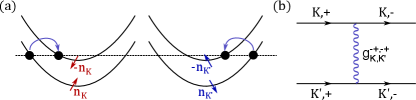
Figure 3: One-magnon exchange processes. (a) Illustration of the momentum-space kinematics and (b) Feynman diagram for one-magnon pair scattering. Such events do not take advantage of low-energy Goldstone modes in the spin-canted phase, and thus do not account for spin-orbit-enabled superconductivity in rhombhedral graphene.

Typically, as in standard phonon-mediated pairing, attraction is generated by exchanging one boson. Our problem also supports a process of this type wherein Cooper pairs exchange one magnon; see Fig. 3(b), which represents a magnon-mediated pair scattering event between majority and minority bands. Note in particular that the spin for each valley flips, as required by the transverse nature of the magnon modes that we have retained. Such a process must in turn transfer a large momentum via the exchanged magnon as highlighted above, leading to various challenges for pairing that we now enumerate.

One clear issue is that the pairing interaction does not directly utilize the ${\boldsymbol{q}}=0$ part of the magnons, and therefore cannot qualitatively distinguish between gapless and gapped branches. The “on-Fermi-surface” Cooper-pair scattering amplitudes arising from exchange of a single magnon of any type are correspondingly non-singular in the low-frequency limit. Consider, for instance, the Goldstone mode labeled $s-$. At small momenta, $|{\boldsymbol{q}}|\lesssim q_{\rm max}$, the $s-$ mode is low-energy and linearly dispersing, and mediates scattering amplitudes calculated in Eq. (37). At larger $|{\boldsymbol{q}}|$, however, $s-$ acquires a quadratic dispersion and bends upward, reaching an energy scale comparable to the Fermi energy at $|{\boldsymbol{q}}|\sim k_{F}$. Repeating the analysis of Sec. III in the latter regime, we find that the typical “on-Fermi-surface” pair scattering amplitude is modified,

$$g^{-+,-+}_{K,K^{\prime}}(\nu,|{\boldsymbol{q}}|\sim k_{F})\sim\frac{1}{-i\gamma\nu+Dk_{F}^{2}}.$$ (42)

The $k_{F}$ factor invariably preempts any low-frequency divergence in the pairing interaction mediated by one $s-$ magnon; similar conclusions hold for the other branches.

The non-singular nature of the one-magnon pairing interactions already justifies focusing on two-magnon processes—which we show in the next subsection do generate a low-frequency divergence. Nevertheless, it is worth highlighting additional issues with this scenario. As a reminder, to achieve pairing in the presence of strong Coulomb repulsion, usually one invokes the Anderson-Morel picture: pair-breaking effects of Coulomb are suppressed when the Fermi energy $\epsilon_{F}$ greatly exceeds the bandwidth of the pairing interaction (i.e., when the pairing interaction exhibits strong retardation). This regime holds for phonon-mediated attraction, whose bandwidth is set by the Debye frequency that is much lower than $\epsilon_{F}$. However, in the one-magnon exchange scenario, the bandwidth of the pairing interaction is set by the magnon energy which, as noted above, is expected to be comparable to $\epsilon_{F}$. Indeed Eq. (42) is a Lorentzian function of $\nu$ with a bandwidth $\propto\epsilon_{F}$. Thus it is far from obvious that attraction from this subdominant channel could yield superconductivity in the presence of Coulomb repulsion.

Finally, the one-magnon scenario does not naturally explain the observed superconducting phenomenology in graphene multilayers. Only large-momentum magnons participate, whose energy are similar with and without spin-orbit interaction, and regardless of whether the parent normal state exhibits spin-canting order. In sharp contrast, experiments indicate that proximity-induced spin-orbit coupling plays a decisive role in promoting Cooper pairing.

IV.2 Two-magnon exchange scenario

So far we have shown that a traditional scenario where Cooper pairs exchange one magnon does not compellingly explain superconductivity emerging from a spin-canted phase. Can the Goldstone mode then provide a viable pairing glue? In this subsection, we definitively answer this question ‘yes’ and show that, as claimed earlier, the dominant attraction channel arises from two small-momentum magnon exchanges, where the first exchange brings Cooper pairs to high-energy states and the second brings them back to the Fermi level; recall Fig. 4(a).

Let us start by calculating the pairing interaction generated by two-magnon exchanges. Since the bare magnon-mediated interactions from Eq. (33) generate high-energy states at small $q$, one can treat $\mathcal{S}_{I}$ in perturbation theory when focusing on soft-magnon contributions. At second order one obtains an intervalley four-fermion interaction that, after projecting onto the pairing channel, can be expressed as

$$\mathcal{S}^{\text{2-mag}}_{\rm pair}=-\sum_{\alpha=\pm}\int_{kq}g^{(2)}_{\Phi}(q)\overline{\Phi}^{\alpha}_{k+q}\Phi^{\alpha}_{k},$$ (43)

where we defined the Cooper pair field $\Phi^{\alpha}_{k}=\Psi_{\alpha K^{\prime},-k}\Psi_{\alpha K,k}$, with $\alpha=\pm$ denoting the majority ($+$) or minority ($-$) band. The coupling function $g_{\Phi}^{(2)}(q)$ turns out to be $\alpha$-independent within our approximations. In the convention specified above, positive values of $g_{\Phi}^{(2)}$ correspond to attractive interactions. We shall see below that $g_{\Phi}^{(2)}$ is indeed positive regardless of the sign of each scattering amplitude because it involves two magnons.

The two-magnon pairing interaction in Eq. (43) can be expressed through irreducible second-order diagrams as shown in Fig. 4; the associated small-$q$ scattering amplitudes $g^{\alpha^{\prime}\alpha,\beta^{\prime}\beta^{\prime}}_{\xi_{1},\xi_{2}}$ are given in Eq. (37). The figure illustrates three types of processes: (a) the ladder diagram and (b) the crossed or “exchange” diagram, that correspond to virtual pair scattering, and (c) vertex corrections or “wineglass” diagrams.

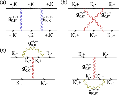
Figure 4: Pairing interaction mediated by two-magnon exchanges. Three types of two-magnon processes are given by (a) the ladder diagram, (b) the cross diagram, and (c) vertex corrections. Solid lines represent electrons near the Fermi surface that can form Cooper pairs, while dashed lines represent virtual excitations in the intermediate stages; see Fig. 1(b). Wiggly lines represents magnon-mediated interactions of three types. Blue lines ($g^{+-,+-}_{K,K^{\prime}}$ and $g^{-+,-+}_{K,K^{\prime}}$) and red lines ($g^{+-,-+}_{K,K^{\prime}}$ and $g^{-+,+-}_{K,K^{\prime}}$) represent intervalley scatterings, while yellow lines represents intravalley scatterings.

Vertex corrections suffer from the same issue as the first-order diagrams—namely, they require a large momentum transfer that does not directly benefit from the long-wavelength Goldstone mode. Vertex corrections thus also exhibit a broad bandwidth and, most importantly, their contribution is non-divergent at low frequency and therefore negligible compared to the other second-order diagrams.

We turn now to the pairing interactions generated by the ladder diagram $g_{\rm l}^{(2)}$ and cross diagram $g_{\rm x}^{(2)}$, which can be expressed as

$$g^{(2)}_{\rm l}(q) =\frac{1}{4\bar{m}^{2}}\int_{Q}g^{+-,+-}_{K,K^{\prime}}(Q+q)g^{-+,-+}_{K,K^{\prime}}(-Q),$$ (44)

$$g^{(2)}_{\rm x}(q) =\frac{1}{4\bar{m}^{2}}\int_{Q}g^{+-,-+}_{K,K^{\prime}}(Q+q)g^{-+,+-}_{K,K^{\prime}}(-Q),$$ (45)

where we defined the short-hand $Q\equiv(i\Omega,{\boldsymbol{Q}})$ [56]. Using the small-$q$ asymptotic expressions for $g^{+-,-+}_{K,K^{\prime}}$ and $g^{-+,-+}_{K,K^{\prime}}$ given in Eq. (37), we see that these two diagrams yield identical contributions; together they dominate the two-magnon pairing interaction

$$g_{\Phi}^{(2)}(q)=g^{(2)}_{\rm l}(q)+g^{(2)}_{\rm x}(q)$$ (46)

$$\sim\frac{\cos^{4}\theta_{0}}{8\bar{m}^{2}z_{s}^{2}\kappa^{2}}\int_{Q}\frac{1}{(\Omega+\nu)^{2}+c_{s}^{2}|{\boldsymbol{Q}}+{\boldsymbol{q}}|^{2}}\frac{1}{\Omega^{2}+c_{s}^{2}|{\boldsymbol{Q}}|^{2}}.$$

Power-counting provides a shortcut to see that $g_{\Phi}^{(2)}$ diverges as $q\rightarrow 0$. Namely, there are three integrals (one frequency, two momentum components), whereas the denominator of the integrand is quadratic in $\nu$ and ${\boldsymbol{q}}$. Thus the pairing interaction should scale as $\sim 1/\nu$ at small $\nu$ with ${{\boldsymbol{q}}}=0$, and as $\sim 1/|{\boldsymbol{q}}|$ at small ${\boldsymbol{q}}$ with $\nu=0$. We substantiate this argument in Appendix E by evaluating the integrals in the following two extreme regimes:

$$g_{\Phi}^{(2)}(q)\sim\begin{cases}\frac{I}{c_{s}|{\boldsymbol{q}}|},&\nu\ll c_{s}|{\boldsymbol{q}}|\\ \frac{I}{\nu},&\nu\gg c_{s}|{\boldsymbol{q}}|\end{cases},~{}~{}I=\frac{V+J}{16z_{s}D}\cos^{2}\theta_{0}.$$ (47)

To proceed analytically while preserving the preceding IR divergences, we substitute $g_{\Phi}^{(2)}(q)$ with the expression

$$g_{\Phi}^{(2)}(q)\rightarrow\frac{I}{\sqrt{\nu^{2}+c_{s}^{2}|{\boldsymbol{q}}|^{2}}}.$$ (48)

As this pairing interaction does not exhibit any sign alternation in momentum space, we focus below on $s$-wave pairing that is expected to dominate. There are two $s$-wave channels to consider: one on the majority Fermi surfaces $(+)$ and the other on the minority Fermi surfaces $(-)$. The effective $s$-wave interactions in these two channels are simply given by the average of $g_{\Phi}^{(2)}(q)$ over the corresponding Fermi surfaces:

$$\overline{g_{\Phi,\pm}^{(2)}}(\nu) =\int\frac{dq_{\parallel}}{2\pi k_{F}^{\pm}}g_{\Phi}^{(2)}(\nu,(q_{\parallel},q_{\perp}=0)).$$ (49)

Here $q_{\parallel}$ and $q_{\perp}$ denote momentum components parallel and normal to the Fermi surface exhibiting Fermi momentum $k_{F}^{\alpha}$ in band $\alpha$. Upon working out this integral we find a logarithmic divergence in the low-frequency limit,

$$\overline{g_{\Phi,\pm}^{(2)}}(\nu)\sim\frac{\cos\theta_{0}}{64\pi\bar{m}k_{F}^{\pm}}\sqrt{\frac{V+J}{z_{s}D^{3}}}\ln\left(\frac{c_{s}q_{\rm max}}{|\nu|}\right),$$ (50)

with $q_{\rm max}=\frac{1}{V}\sqrt{\frac{J}{D}}\cos\theta_{0}$ the momentum cutoff below which the dispersion of the $s-$ magnon mode is linear. This interaction is attractive and therefore catalyzes $s$-wave pairing mediated by two-magnon exchange. Importantly, the logarithmic divergence at low frequency renders the interaction narrow-band, and therefore pairing resulting from this mechanism more readily survives bare Coulomb repulsion through the Anderson-Morel mechanism.

The $\cos\theta_{0}$ factor in Eq. (50) translates into a linear dependence on $\lambda_{I}$ using the saddle-point condition Eq. (13), thus linking spin-orbit coupling with enhanced pairing. In the $\theta_{0}\rightarrow 0$ limit where spin-canting order disappears in favor of spin-valley locking, we have shown in Sec. III.2 that the additional gapless (critical) mode at the transition yields intervalley magnon interactions with the same frequency and momentum structure as in the generic canting case, albeit with different amplitudes. In this limit only the ladder diagrams in Fig. 4(b) contribute, ultimately leading to a pairing interaction identical to Eq. (50) but with $\cos\theta_{0}\rightarrow 1$. Our mechanism thus predicts a saturation of the pairing strength when increasing $\lambda_{I}$ towards the canting transition. However, when the spin-valley locked phase is nucleated, we expect superconductivity to quickly evaporate as all collective modes becomes gapped—see also Fig. 2.

Within the weak-coupling BCS framework, the $s$-wave pairing gap $\Delta_{\pm}$ for the majority ($+$) and minority ($-$) bands is determined by the gap equations

$$\Delta_{\pm}(\omega)=\mathcal{N}_{\pm}\int_{\nu}\overline{g_{\Phi,\pm}^{(2)}}(\omega-\nu)\frac{\Delta_{\pm}(\nu)}{\sqrt{\nu^{2}+\Delta_{\pm}^{2}(\nu)}},$$ (51)

with $\mathcal{N}_{\pm}$ the density of states at the corresponding Fermi surfaces. Here, we only account for the leading contribution from two-magnon interactions; moreover, we have neglected self-energy corrections (which we discuss in Sec. V). The two gaps $\Delta_{\pm}$ decouple at this level, though they will mix by subleading interactions (e.g., one-magnon exchange) that provide residual Josephson coupling between the bands. We stress that $\overline{g_{\Phi,\pm}^{(2)}}$ is inversely proportional to the Fermi surface radius; recall Eq. (50). This unusual feature arises because the zero-frequency pairing interaction is strongly peaked near momentum transfer ${\boldsymbol{q}}=0$—in contrast to, e.g., acoustic phonons for which $g_{\rm ph}(\nu=0,{\boldsymbol{q}})$ is nearly momentum-independent. Assuming the density of states $\mathcal{N}_{\pm}$ are comparable, stronger pairing is correspondingly expected for the minority carriers. This prediction is in harmony with observations in spin-orbit-proximitized graphene multilayers, where superconductivity appears in parameter regimes featuring minority pockets; for further discussion on this important point see Sec. VI.

We have now seen that the one-magnon scenario faces issues that two-magnon processes remedy. A crucial question remains, however: Can higher-order magnon-exchange events produce even stronger contributions, potentially dooming the entire perturbative framework? Fortunately, higher-order diagrams do not exhibit a low-frequency divergence and are thus negligible compared to those that involve two magnons. This result can be seen by power counting: Introducing one more magnon line into the diagrams in Fig. 4 yields two additional powers of momentum and frequency in the denominator of the integrand—yet also introduces extra integrals along three dimensions (one frequency, two momentum components). Higher-order diagrams are therefore less divergent compared to those arising at second order. Given that $\overline{g_{\Phi}^{(2)}}(\nu)$ is merely logarithmically divergent, we conclude that the momentum-averaged pairing interaction arising from higher-order diagrams is indeed non-divergent.

IV.3 Suppression of pairing interaction in the absence of spin-orbit coupling

In the previous subsection we considered generic canting angles as well as the special limit $\theta_{0}\rightarrow 0$. Here we focus on the $\theta_{0}\rightarrow\pi/2$ limit, corresponding to a vanishing spin-orbit interaction $\lambda_{I}\rightarrow 0$, which may be relevant for experiments without a neighboring TMD. In this limit, the leading contribution to the interaction in Eq. (50) vanishes due to the $\cos\theta_{0}$ factor. The physical interpretation of this behavior can be traced back to the disappearance of linearly dispersing Goldstone magnons; the magnon dispersion becomes quadratic as the microscopic Hamiltonian preserves SU(2) rather than U(1) symmetry.

To understand the fate of pairing in the $\theta_{0}=\pi/2$, spin-orbit-free limit, we calculate the two-magnon interaction generated by the quadratically dispersing modes at small ${\boldsymbol{q}}$ [recall Eq. (41)]. Only the crossed diagrams in Fig. 4(b) contribute, due to symmetry considerations described above that kill vertices that change the total spin projection along the in-plane polarization axis. The pairing interaction thus reads

$$g^{(2)}_{\Phi,\frac{\pi}{2}}(q)\sim\frac{1}{4\bar{m}^{2}}\int_{Q}\frac{1}{-i\gamma(\Omega+\nu)+D({\boldsymbol{Q}}+{\boldsymbol{q}})^{2}}\frac{1}{i\gamma\Omega+D{\boldsymbol{Q}}^{2}}.$$ (52)

The above integral can be computed exactly; see Appendix E.2. Focusing on $\nu=0$ (i.e., magnon-mediated interactions resonant on the Fermi surface), we obtain

$$g^{(2)}_{\Phi,\frac{\pi}{2}}(\nu=0,{\boldsymbol{q}})\sim\frac{V+J}{8\pi D\bar{m}}\ln\frac{2\Lambda}{|{\boldsymbol{q}}|},$$ (53)

where $\Lambda$ is a momentum cut-off related to the finite bandwidth of the quadratically dispersing magnon modes.

Contrary to the generic spin-canting result in Eq. (48), this zero-frequency interaction is only logarithmically divergent at small momentum. Consequently, its momentum-averaged value is finite and subdominant relative to the $\lambda_{I}\neq 0$ case. That is, spin-orbit interaction qualitatively enhances $s$-wave superconductivity mediated by two-magnon exchange—also in harmony with rhombohedral graphene experiments.

V Does Pairing survive self-energy?

In Sec. IV.2 we established that the momentum-averaged pairing interaction arising from the two-magnon scenario is attractive and log-divergent at low frequency, yielding $s$-wave superconductivity within a weak-coupling BCS framework (see Eq. 51). Caution is warranted, however, as the presence of a singular pairing interaction might also lead to a singular imaginary part of the electron self-energy $\Sigma(i\nu)$. Furthermore, $\Sigma(i\nu)$ affects the coherence of fermions and blurs the Fermi surface—thus generally competing with pairing, as the latter relies on the energy gain from gapping out a sharp Fermi surface. A similar situation appears in quantum critical pairing scenarios [57, 58, 59, 60, 61, 62, 63, 64, 65, 65, 66], where a quantum critical mode mediates a singular pairing interaction as well as a singular imaginary part of the self-energy. In this section we address two questions: Is the self-energy actually singular in our problem? And if so, does the tendency towards pairing or towards non-Fermi liquid behavior win out?

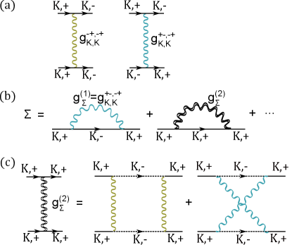
Figure 5: Self-energy from magnon-mediated interactions. (a) Two types of intravalley scattering processes appearing in the self-energy. (b) Self-energy contributions arise from a one-magnon effective interaction $g_{\Sigma}^{(1)}$, a two-magnon interaction $g_{\Sigma}^{(2)}$, and those from higher orders (denoted by the ellipsis). The one-magnon piece $g^{(1)}_{\Sigma}$ simply corresponds to the intravalley scattering amplitude $g^{+-,-+}_{K,K}$. The two-magnon piece $g^{(2)}_{\Sigma}$ (double wiggly black lines) is given by the two diagrams in panel (c). These diagrams are similar to those in the two-magnon pairing interaction—recall Fig. 4—except that only intravalley scattering processes are involved.

Unlike in problems studied in the literature such as Refs. 67, where the divergent pairing interaction directly generates a singular self-energy, in our problem the self-energy originates from a series of processes distinct from the pairing interaction. Figure 5 illustrates the self-energy-generating diagrams at each order $g_{\Sigma,\alpha}^{(n)}$ ($n=1,2,...$), which are structurally similar to those of the pairing interaction at order $g_{\Phi}^{(n)}$. However, the magnon lines (wiggly lines) in the pairing and self-energy correspond to different scattering types. In the pairing interaction, wiggly lines represent intervalley processes whereas in the self-energy, wiggly lines represent intravalley processes. For generic $\theta_{0}$ values away from 0 and $\pi/2$, this distinction nevertheless does not affect the leading divergence of the self-energy: As shown in Sec. III.1 the asymptotic expressions for intervalley $g_{K,K^{\prime}}$ and intravalley $g_{K,K}$ amplitudes are identical [Eq. (37)].

We thus conclude that the interactions $g_{\Sigma,\alpha}^{(n)}$ that govern the self-energies are asymptotically identical to the pairing interactions $g_{\Phi,\alpha}^{(n)}$. The leading contribution also occurs at the two-magnon level [see Fig. 5(c)], with $g_{\Sigma,\alpha}^{(2)}$ diverging logarithmically at low frequency. A straightforward calculation shows that the self-energies $\Sigma_{\alpha}$ ($\alpha=\pm$) feature the following leading singularity,

$$\Sigma_{\alpha}(i\omega)\sim-i\mathcal{N}_{\alpha}{\rm sgn}(\omega)\int^{|\omega|}_{0}\overline{g_{\Sigma,\alpha}^{(2)}}(\nu)d\nu\propto-i\omega\ln\frac{\omega_{*}}{|\omega|},$$ (54)

where $\omega_{*}$ is a frequency cutoff and $\overline{g_{\Sigma,\alpha}^{(2)}}$ denotes an average of the corresponding amplitude over the $\alpha$ Fermi surface. In contrast, the first-order diagram in Fig. 5(b) does not give a singular self-energy contribution because the interaction scatters an electron between the $+$ and $-$ Fermi surfaces, which requires a large momentum transfer.

Interestingly, the situation of ${\rm\,Im\,}\Sigma(i\omega)\sim\omega\ln|\omega|$ described in Eq. (54) shows that the normal (non-superconducting) state realizes a marginal Fermi liquid[68]. This situation resembles the rather different problem of conventional boson-mediated pairing in three dimensions. Reference 69 in particular established that exchanging one boson similarly mediates a log-divergent pairing interaction as well as a self-energy with $\omega\ln|\omega|$ singularity—though $T_{c}$ for pairing is still nonvanishing. We therefore conclude that pairing also occurs in our two-dimensional, two-magnon-exchange scenario despite the singular self-energy. We note that, since $g_{\Sigma}^{(n)}$ is asymptotically identical to $g_{\Phi}^{(n)}$, the fate of the self-energy generated at third-order or higher is similar to that of the high-order irreducible pairing interaction—such corrections are also non-divergent and therefore negligible compared to the two-magnon ones.

VI Discussion

Our theory admits several experimentally testable predictions. We start by discussing the dependence of superconductivity on Ising spin-orbit coupling strength $\lambda_{I}$, which naturally accommodates two seemingly contradictory behaviors:

1. The phase diagram area populated by superconductivity shrinks upon increasing spin-orbit coupling. In our scenario the pairing glue—soft magnons—relies on spin-canting order in the normal state. As $\lambda_{I}$ increases, however, canting order eventually loses in favor of an Ising spin-valley-locked phase; recall Sec. II.1. It is thus natural to anticipate that the spin-canting phase occupies a progressively smaller region of the phase diagram as $\lambda_{I}$ rises, as also seen in Hartree-Fock studies [48]. Our theory then predicts that superconductivity should also occupy a diminished area.

2. The critical temperature $T_{c}$ is enhanced upon increasing the spin-orbit coupling. This prediction follows directly from our analysis of the pairing interaction in Eq. (50), which contains a $\cos\theta_{0}\propto\lambda_{I}$ prefactor. This factor vanishes when $\lambda_{I}\rightarrow 0$, i.e., the divergence that drives two-magnon-mediated pairing in our scenario disappears. It is then natural that turning on $\lambda_{I}$ increases the optimal $T_{c}$ emerging from a spin-canted normal state, even though the latter’s phase space diminishes.

Remarkably, Ref. 38 observed both of these trends in bilayer devices, where the strength of Ising spin-orbit interaction was controlled through engineering the twist angle at the WSe₂-graphene interface [70, 71, 72]. Direct detection of the spin-canting order central to our theory (e.g., by SQUID measurements) poses arguably the simplest falsifiable check for our proposed explanation.

Another nontrivial prediction concerns the dependence of superconductivity on carrier density. We showed that our proposed two-magnon exchange mechanism activates two $s$-wave pairing channels—one for the majority Fermi surfaces, and the other for the minority Fermi surfaces. Importantly, we find that the pairing interaction scales inversely proportional to the corresponding Fermi momenta, implying that pairing predominantly occurs in the minority species with a strength that—all other factors, e.g. density of states, being equal—grows when the minority carrier density decreases. This prediction indeed matches the generic behavior observed in bilayer and trilayer graphene where prominent superconducting phases appear in regions hosting small pockets [36, 37, 38, 39, 40, 41]; perhaps even more strikingly, in trilayers these regions abruptly terminate near Lifshitz transitions marking the disappearance of minority carriers [40, 41].

Our pairing scenario also has ramifications for depairing by in-plane magnetic fields $B_{\parallel}$. Conventional in-plane-field depairing mechanisms include orbital effects and warping of the Fermi surfaces due to an interplay with Rashba spin-orbit coupling [73] (which we have neglected so far but discuss further below). Magnon-mediated pairing admits a qualitatively different depairing effect: Namely, $B_{\parallel}$ explicitly breaks the U(1) spin-rotation symmetry that the spin-canting phase breaks spontaneously—thereby generating a gap $\Delta_{\rm mag}\sim\sqrt{|B_{\parallel}|}$ for the Goldstone magnon mode. (Imagine the potential utility of an experimental knob for controllably gapping out phonons in conventional superconductors!) As explained in Appendix E.3, the field-induced gap regularizes the low-frequency divergence of the pairing interaction in Eq. (50) via the replacement $|\nu|\rightarrow|\nu|+\Delta_{\rm mag}$. The resulting dependence of $T_{c}$ on $B_{\parallel}$ poses a nontrivial problem worth future study, as it requires solving frequency-dependent Eliashberg equations, also accounting for the self-energy whose singularity at small ${\boldsymbol{q}}$ will be similarly cut off by $B_{\parallel}$. Nevertheless, we can at least qualitatively assert that our mechanism implies greater susceptibility to in-plane depairing effects compared to, say, a phonon-mediated scenario, possibly explaining peculiar Pauli-limit violation trends observed experimentally [36, 37, 39, 40].

As alluded to above, Rashba spin-orbit coupling $\lambda_{R}$ generically accompanies Ising spin-orbit interaction in graphene multilayers proximitized by a TMD. And like in-plane magnetic fields, $\lambda_{R}$ explicitly breaks U(1) spin symmetry, gapping the Goldstone magnon even at $B_{\parallel}=0$. The bare Rashba energy scale is believed to be relatively weak, $\lambda_{R}\sim 1~{}\rm{meV}$, in graphene devices proximitized by WSe₂ or WS₂ [29, 30, 31, 32, 33, 34, 35, 70, 71, 72]. Crucially, however, the effective Rashba spin splitting in the low-energy bands strongly depends on the applied displacement field and the fermiology of the pockets relevant for pairing—and should be most prominent in large Fermi pockets. In our mechanism small Fermi pockets are favored (due to the $1/k_{F}$ dependence in the pairing interaction), which are predicted to be much less sensitive to Rashba depairing effects. In principle, measuring devices with variable $\lambda_{R}$, and ideally other parameters fixed, would provide another falsifiable check for our theory.

We conclude with some speculation on extensions of our theory. Analyzing the favorability of spin-canting order in systems composed of more than three graphene layers, e.g., from a Hartree-Fock angle, would provide valuable insight into the wider applicability of our proposed pairing mechanism. It is also interesting to explore pairing mediated by Goldstone modes associated with other broken-symmetry orders, most notably intervalley coherence that also naturally emerges in graphene multilayers [12, 46, 74, 48, 75]. A particularly interesting possibility—which combines the two different types of continous symmetry breaking relevant for graphene systems—consists of intervalley coherent orders that also exhibit spin canting [76]. Such composite order can lead to generalized quarter-metal states that comprise a single, non-degenerate majority Fermi surface; similarly to the ideas developed in this work, our two-magnon exchange mechanism could potentially mediate Cooper pairing in this setting. Interestingly, one of the new superconducting regions in proximitized Bernal bilayer graphene [36] exhibits fermiology consistent with this description.

Looking beyond graphene, can one identify a broader set of candidate materials for which Cooper pairing emerges from two-magnon exchange processes boosted by spin-orbit interaction? Ferromagnetic bulk materials composed of weakly coupled layers may be fruitful in this regard. In particular, the magnetic order could inherit a spin-canted structure upon introducing spin-orbit coupling; moreover, the layering could potentially allow magnons to mediate singular pairing interactions as in our analysis. For systems realizing more complex magnetic order (e.g., antiferromagnetism), can two-magnon exchange still provide a fruitful pairing mechanism—possibly leading to superconducting order parameters beyond simple $s$-wave? Finally, can one uncover excitonic analogues of our magnon-mediated pairing scenario?

Appendix A Calculation of spin susceptibilities

Below we calculate the transverse spin susceptibilities $\chi_{1}$ and $\chi_{2}$ defined in Eqs. (20) and (21):

$$\chi_{1}(i\nu,{\boldsymbol{q}})= -\int_{p}\left[G_{\xi,+}(p+q)G_{\xi,-}(p)+G_{\xi,-}(p+q)G_{\xi,+}(p)\right]$$

$$= -\int_{{\boldsymbol{p}}}T\sum_{\omega}\frac{1}{i\left(\omega+\nu\right)-\epsilon_{\xi,{\boldsymbol{p}}+{\boldsymbol{q}}}+\bar{m}}\frac{1}{i\omega-\epsilon_{\xi,{\boldsymbol{p}}}-\bar{m}}+(\nu\rightarrow-\nu,{\boldsymbol{q}}\rightarrow-{\boldsymbol{q}}),$$

$$= \int_{{\boldsymbol{p}}}\frac{f(\epsilon_{\xi,{\boldsymbol{p}}+{\boldsymbol{q}}}-\bar{m})-f(\epsilon_{\xi,{\boldsymbol{p}}}+\bar{m})}{i\nu-\left(\epsilon_{\xi,{\boldsymbol{p}}+{\boldsymbol{q}}}-\epsilon_{\xi,{\boldsymbol{p}}}\right)+2\bar{m}}+(\nu\rightarrow-\nu,{\boldsymbol{q}}\rightarrow-{\boldsymbol{q}}),$$

$$= ~{}C_{0}-\kappa\nu^{2}-D{\boldsymbol{q}}^{2},$$ (55)

$$\chi_{2}(i\nu,{\boldsymbol{q}})= i\int_{p}[G_{\xi,+}(p+q)G_{\xi,-}(p)-G_{\xi,-}(p+q)G_{\xi,+}(p)]$$

$$= i\int_{{\boldsymbol{p}}}T\sum_{\omega}\frac{1}{i\left(\omega+\nu\right)-\epsilon_{\xi,{\boldsymbol{p}}+{\boldsymbol{q}}}+\bar{m}}\frac{1}{i\omega-\epsilon_{\xi,{\boldsymbol{p}}}-\bar{m}}-(\nu\rightarrow-\nu,{\boldsymbol{q}}\rightarrow-{\boldsymbol{q}}),$$

$$= -i\int_{{\boldsymbol{p}}}\frac{f(\epsilon_{\xi,{\boldsymbol{p}}+{\boldsymbol{q}}}-\bar{m})-f(\epsilon_{\xi,{\boldsymbol{p}}}+\bar{m})}{i\nu-\left(\epsilon_{\xi,{\boldsymbol{p}}+{\boldsymbol{q}}}-\epsilon_{\xi,{\boldsymbol{p}}}\right)+2\bar{m}}-(\nu\rightarrow-\nu,{\boldsymbol{q}}\rightarrow-{\boldsymbol{q}}),$$

$$= ~{}-\gamma\nu+O(|{\boldsymbol{q}}|^{3},\nu^{3}).$$ (56)

In the last line of Eqs. (55) and (56) we have performed an expansion to leading order in frequency and momentum. Note that while $\chi_{1}(i\nu,{\boldsymbol{q}})$ is an even function of its arguments, $\chi_{2}(i\nu,{\boldsymbol{q}})$ is an odd function. We further expect the absence of any linear-in-${\boldsymbol{q}}$ term in $\chi_{2}$ due to the model’s rotation symmetry, together with analyticity of $\chi_{2}(q)$; the latter property precludes a $\sim|{\boldsymbol{q}}|$ contribution.

The expression for the parameter $D$ is complicated and depends on the detail of band dispersion, so we do not write it down explicitly. On the other hand, the parameters $C_{0}$, $\kappa$ and $\gamma$ can be computed straightforwardly from the ${\boldsymbol{q}}=0$ limit of the above expressions:

$$\chi_{1}(i\nu,0) =\int_{{\boldsymbol{p}}}\frac{f(\epsilon_{\xi,{\boldsymbol{p}}}-\bar{m})-f(\epsilon_{\xi,{\boldsymbol{p}}}+\bar{m})}{i\nu+2\bar{m}}+(\nu\rightarrow-\nu)$$

$$\approx\int_{{\boldsymbol{p}}}\frac{f(\epsilon_{\xi,{\boldsymbol{p}}}-\bar{m})-f(\epsilon_{\xi,{\boldsymbol{p}}}+\bar{m})}{2\bar{m}}\left\{\left(1-\frac{i\nu}{\bar{2m}}-\frac{\nu^{2}}{4\bar{m}^{2}}+\ldots\right)+\left(1+\frac{i\nu}{2\bar{m}}-\frac{\nu^{2}}{4\bar{m}^{2}}+\ldots\right)\right\}$$

$$=\frac{n_{0}}{\bar{m}}-\frac{n_{0}}{4\bar{m}^{3}}\nu^{2},$$ (57)

where $n_{0}=\int_{{\boldsymbol{p}}}\left[f(\epsilon_{\xi,{\boldsymbol{p}}}-\bar{m})-f(\epsilon_{\xi,{\boldsymbol{p}}}+\bar{m})\right]$ denotes the polarization density, i.e., the density difference between the majority and minority spin flavors in each valley. Using the same low-frequency expansion we obtain

$$\chi_{2}(i\nu,0) =-i\int_{{\boldsymbol{p}}}\frac{f(\epsilon_{\xi,{\boldsymbol{p}}}-\bar{m})-f(\epsilon_{\xi,{\boldsymbol{p}}}+\bar{m})}{i\nu+2\bar{m}}-(\nu\rightarrow-\nu)\approx-\frac{n_{0}}{2\bar{m}^{2}}\nu.$$ (58)

From these results we extract coefficients

$$C_{0}=\chi_{1}(0,0)=\frac{n_{0}}{\bar{m}}=\frac{1}{V+J},\quad\kappa=\frac{n_{0}}{4\bar{m}^{3}}=\frac{1}{4(V+J)\bar{m}^{2}},\quad\gamma=\frac{n_{0}}{2\bar{m}^{2}}=\frac{1}{2(V+J)\bar{m}}=2\kappa\bar{m}.$$ (59)

Above we used the saddle-point condition from Eq. (15) to simplify $C_{0}$, $\kappa$ and $\gamma$, leading to the expressions quoted in the main text.

Appendix B Diagonalization of magnon action

The magnon action in Eq. (24) takes the diagonal form in Eq. (26) under a basis rotation

$$\delta M_{s,a}(q)=\left[\begin{matrix}\delta m^{\phi}_{s,a}(q)\\ \delta m^{\theta}_{s,a}(q)\end{matrix}\right]=U_{s,a}(\nu)\left[\begin{matrix}\delta m_{s,a+}(q)\\ \delta m_{s,a-}(q)\end{matrix}\right].$$ (60)

Our aim is to explore low-frequency properties of the matrix $U_{s,a}(\nu)$, which is composed of (right) eigenvectors of the $2\times 2$ matrices appearing in Eq. (24). For generic canting angles $\theta_{0}$ not too close to $0$ or $\pi/2$, the only low-energy magnon mode corresponds to the $s-$ branch. The corresponding eigenvector is given by

$$\Phi_{s-}(\nu)=\frac{1}{\sqrt{\mathcal{N}}}\left[\begin{matrix}\tilde{J}\cos^{2}\theta_{0}+\sqrt{(\tilde{J}\cos^{2}\theta_{0})^{2}-(\gamma\nu)^{2}}\\ \gamma\nu\end{matrix}\right]$$ (61)

with $\mathcal{N}$ a normalization factor. For low frequencies satisfying $\gamma\nu\lesssim\tilde{J}\cos^{2}\theta_{0}$, to a good approximation only the upper entry survives, and one can simply take $\Phi_{s-}(\nu)\approx\left[\begin{matrix}1\\ 0\end{matrix}\right]$. That is, at low frequencies the Goldstone mode has weight primarily on the $\delta m_{s}^{\phi}(q)$ fluctuation field.

For $\theta_{0}=0$, the $a-$ branch joins $s-$ as a second gapless mode. The $a-$ eigenvector is

$$\Phi_{a-}(\nu)=\frac{1}{\sqrt{\mathcal{N}^{\prime}}}\left[\begin{matrix}\tilde{J}-\sqrt{\tilde{J}^{2}-(\gamma\nu)^{2}}\\ -\gamma\nu\end{matrix}\right],$$ (62)

where $\mathcal{N}^{\prime}$ again represents a normalization factor. At low frequencies satisfying $\gamma\nu\lesssim\tilde{J}^{2}$, the upper entry is now subdominant, and hence in this regime we have $\Phi_{a-}(\nu)\approx\left[\begin{matrix}0\\ 1\end{matrix}\right]$. The gapless $a-$ mode thus has weight primarily on the $\delta m_{a}^{\theta}(q)$ fluctuation field.

Finally, at $\theta_{0}=\pi/2$, one must consider both the $s-$ and $s+$ branches, with eigenvectors

$$\Phi_{s-}(\nu)=\frac{1}{\sqrt{2}}\left[\begin{matrix}1\\ -i{\rm sgn}(\nu)\end{matrix}\right],~{}~{}~{}~{}~{}~{}\Phi_{s+}(\nu)=\frac{1}{\sqrt{2}}\left[\begin{matrix}1\\ +i{\rm sgn}(\nu)\end{matrix}\right].$$ (63)

Contrary to the cases examined above, these modes admit equal weight on the $\delta m^{\phi}_{s}$ and $\delta m^{\theta}_{s}$ fields (for any nonzero frequency). We stress that one should not view $s+$ as a mode that gradually evolves from gapped to gapless as $\theta_{0}$ approaches $\pi/2$. Rather, the $s+$ abruptly acquires a low-frequency, low-momentum pole precisely at $\theta_{0}=\pi/2$. See the following appendix for more discussion.

Appendix C Dispersion of magnons

In the main text, we obtained magnon propagators

$$\mathcal{G}_{b\eta}(q) =2\left[Q^{\phi}_{b}+Q^{\theta}_{b}+\eta\sqrt{(Q^{\phi}_{b}-Q^{\theta}_{b})^{2}-(2\gamma\nu)^{2}}\right]^{-1}$$ (64)

with $b=s,a$ and $\eta=\pm$. We now solve for the low-energy magnon spectrum by examining the poles of these propagators. Specifically, we focus on the $s-$ and $a-$ branches since the former is gapless throughout the spin canted phase while the latter becomes gapless at the spin-canting phase transition. We generally ignore the gapped $s+$ and $a+$ branches (but see below for the special case of $\theta_{0}=\pi/2$). Solving the poles at small $q$ for the $s-$ mode, we find the following dispersion relation:

$$\omega_{s-} =\begin{cases}c_{s}|{\boldsymbol{q}}|+O(|{\boldsymbol{q}}|^{2}),\quad&0\leq\theta_{0}<\frac{\pi}{2}\\ \frac{D}{\gamma}|{\boldsymbol{q}}|^{2}+O(|{\boldsymbol{q}}|^{4}),\quad&\theta_{0}=\frac{\pi}{2}\end{cases}.$$ (65)

Away from $\theta_{0}=\pi/2$, this mode disperses linearly with magnon velocity

$$c_{s}=\left(\frac{D}{\kappa z_{s}}\right)^{1/2}\cos\theta_{0},\quad z_{s}=\cos^{2}\theta_{0}+\frac{V-J}{2J}.$$ (66)

Recalling the definition $\kappa=[4(V+J)\bar{m}^{2}]^{-1}$, we see that $c_{s}$ reduces to Eq. (29) from the main text in the physically motivated limit $J\ll V$. Similarly, for the $a-$ mode we obtain

$$\omega_{a-}=\sqrt{\Omega_{a-}^{2}+c_{a}^{2}|{\boldsymbol{q}}|^{2}}+O(|{\boldsymbol{q}}|^{4}).$$ (67)

The associated velocity is

$$c_{a} =\left(\frac{D}{\kappa z_{a}}\right)^{1/2}\left(1+\sin^{2}\theta_{0}\right)^{1/2},\quad z_{a}=(1+\sin^{2}\theta_{0})+\frac{V-J}{2J};$$ (68)

moreover, the ${\boldsymbol{q}}=0$ magnon gap reads

$$\Omega_{a-}=\left[\frac{\tilde{J}}{\kappa}(1+\sin^{2}\theta_{0})+\frac{\gamma^{2}}{2\kappa^{2}}-\sqrt{\left(\frac{\tilde{J}}{\kappa}(1+\sin^{2}\theta_{0})+\frac{\gamma^{2}}{2\kappa^{2}}\right)^{2}-\frac{4\tilde{J}^{2}}{\kappa^{2}}\sin^{2}\theta_{0}}\right]^{\frac{1}{2}}$$ (69)

and is generally finite but decreases to zero as $\theta_{0}\rightarrow 0$.

The $s+$ branch warrants further discussion. As alluded to above, $\mathcal{G}_{s+}$ generically exhibits poles corresponding to gapped magnon excitations. The situation should be contrasted to $\mathcal{G}_{a-}$, whose poles indicate that the associated magnon gap decreases continuously as $\theta_{0}$ tends to zero—eventually becoming gapless at the $\theta_{0}=0$ spin canting transition. Right at $\theta_{0}=\pi/2$, however, a low-frequency pole suddenly emerges in $\mathcal{G}_{s+}$. This pole corresponds to the negative-frequency branch of the $s-$ mode, i.e., $\omega_{s+}=-\omega_{s-}$, meaning that $s+$ does not actually constitute a new mode. Nevertheless, the sudden emergence of a low-frequency pole indicates that $\mathcal{G}_{s+}$ needs to be accounted for on the same footing as $\mathcal{G}_{s-}$ when calculating magnon-mediated interactions in the $\theta_{0}=\pi/2$ limit.

Appendix D Derivation of the one-magnon scattering amplitudes in the spin-orbit-free limit

In this Appendix we derive the result in Eq. (41) for the two-magnon-mediated scattering amplitudes in the $\theta_{0}=\pi/2$ limit, appropriate for vanishing spin-orbit interaction. Let us revisit Eq. (24) in the $\theta_{0}=\pi/2$ limit, where $Q^{\phi}_{s}=Q^{\theta}_{s}$. Using the eigenvector basis specified in Eq. (63) one finds magnon Green’s functions

$$\mathcal{G}_{s\pm}(q)\sim(\mp i\gamma|\nu|+D{\boldsymbol{q}}^{2})^{-1}$$ (70)

for the soft magnon branches. Projection onto those modes follows from

$$\delta m^{\phi}_{\xi}(q)\rightarrow\frac{1}{\sqrt{2}}[\delta m_{s-}(q)+\delta m_{s+}(q)]~{},~{}\delta m^{\theta}_{\xi}(q)\rightarrow-\frac{i{\rm sgn}(\nu)}{\sqrt{2}}[\delta m_{s-}(q)-\delta m_{s+}(q)].$$ (71)

The electron-magnon coupling accordingly evolves to

$$\delta{\boldsymbol{m}}_{\xi}(q)\cdot{\boldsymbol{s}}_{\xi}(-q)\rightarrow\frac{1}{\sqrt{2}}\left\{\delta m_{s-}(q)[S^{y}_{\xi}(-q)-i{\rm sgn}(\nu)S^{x}_{\xi}(-q)]+\delta m_{s+}(q)[S^{y}_{\xi}(-q)+i{\rm sgn}(\nu)S^{x}_{\xi}(-q)]\right\},$$ (72)

and after integrating out the magnons we obtain

$$\mathcal{S}_{\rm I}= -\frac{1}{4}\sum_{\xi_{1},\xi_{2}}\int_{q}\{\mathcal{G}_{s-}(q)[S^{y}_{\xi_{1}}(q)+i{\rm sgn}(\nu)S^{x}_{\xi_{1}}(q)][S^{y}_{\xi_{2}}(-q)-i{\rm sgn}(\nu)S^{x}_{\xi_{2}}(-q)]$$

$$+\mathcal{G}_{s+}(q)[S^{y}_{\xi_{1}}(q)-i{\rm sgn}(\nu)S^{x}_{\xi_{1}}(q)][S^{y}_{\xi_{2}}(-q)+i{\rm sgn}(\nu)S^{x}_{\xi_{2}}(-q)]\}.$$ (73)

Comparing to Eq. (33) and expanding the Green’s functions for small $q$ yields the associated scattering amplitudes

$$g^{-+,-+}_{\xi_{1},\xi_{2}}(q)=0,~{}~{}~{}~{}g^{-+,+-}_{\xi_{1},\xi_{2}}(q)\sim-\frac{1}{-i\gamma\nu+D{\boldsymbol{q}}^{2}},$$ (74)

as quoted in Eq. (41) in the main text.

Appendix E Derivation of two-magnon scattering amplitudes

In this Appendix we derive the two-magnon scattering amplitudes used in the main text. We first consider the generic case, and then separately treat the spin-orbit-free limit. We finally discuss how gapping out the Goldstone magnons (using a Zeeman field) regularizes the low-energy divergence of two-magnon scattering amplitudes.

E.1 Generic case

We first analyze the scattering amplitudes in the generic case where $\theta_{0}\neq 0,\pi/2$. As shown in Eqs. (44) and (45) of the main text, the pairing interaction arising from the ladder diagram $g_{\rm l}^{(2)}$ and from the crossed diagram $g_{\rm x}^{(2)}$ are asymptotically the same, since the asymptotic frequency-momentum-dependence of $g^{+-,-+}_{K,K^{\prime}}$ and $g^{+-,-+}_{K,K^{\prime}}$ at small $q$ are identical. The amplitudes of these two processes are given by

$$g^{(2)}_{\rm l}(q)=g^{(2)}_{\rm x}(q)=\frac{\cos^{4}\theta_{0}}{16\bar{m}^{2}z_{s}^{2}\kappa^{2}}\int_{\Omega,{\boldsymbol{Q}}}\frac{1}{(\Omega+\nu)^{2}+c_{s}^{2}({\boldsymbol{Q}}+{\boldsymbol{q}})^{2}}\frac{1}{\Omega^{2}+c_{s}^{2}{\boldsymbol{Q}}^{2}}.$$ (75)

Here, we have used $\Omega\ll\bar{m}$ because the magnon frequency $\Omega$ is much smaller than the Fermi energy, whereas we assume that the polarization field $\bar{m}$ is comparable to the Fermi energy, as inferred from measurements [38]. We now show that $g^{(2)}(q)$ features a singularity at small momentum and frequency by examining two extreme regimes:

1. In the regime of $\nu\ll c_{s}|{\boldsymbol{q}}|$, $g_{l,x}^{(2)}(q)$ can be computed as follows. Taking $\nu=0$ in Eq. (75), we first massage the integrand to make it more symmetric—i.e., we shift the integration variable ${\boldsymbol{Q}}\rightarrow{\boldsymbol{Q}}-{\boldsymbol{q}}/2$ to obtain

   $$g^{(2)}_{\rm l,x}(\nu=0,{\boldsymbol{q}})=\frac{\cos^{4}\theta_{0}}{16\bar{m}^{2}z_{s}^{2}\kappa^{2}}\int_{\Omega,{\boldsymbol{Q}}}\frac{1}{\Omega^{2}+c_{s}^{2}({\boldsymbol{Q}}+\frac{{\boldsymbol{q}}}{2})^{2}}\frac{1}{\Omega^{2}+c_{s}^{2}({\boldsymbol{Q}}-\frac{{\boldsymbol{q}}}{2})^{2}}.$$ (76)

   Taking ${\boldsymbol{q}}$ along the $x$ axis and denoting by $\theta$ the angle measured from ${\boldsymbol{q}}$, we then perform the Matsubara summation to obtain

   $$g^{(2)}_{\rm l,x}(\nu=0,{\boldsymbol{q}})=\frac{\cos^{4}\theta_{0}}{16\bar{m}^{2}z_{s}^{2}\kappa^{2}}\frac{1}{2c_{s}^{3}|{\boldsymbol{q}}|}\int\frac{d|{\boldsymbol{Q}}|d\theta}{4\pi^{2}}\frac{1}{\cos\theta}\left(\frac{1}{\sqrt{{\boldsymbol{q}}^{2}+4{\boldsymbol{Q}}^{2}-4|{\boldsymbol{Q}}||{\boldsymbol{q}}|\cos\theta}}-\frac{1}{\sqrt{{\boldsymbol{q}}^{2}+4{\boldsymbol{Q}}^{2}+4|{\boldsymbol{Q}}||{\boldsymbol{q}}|\cos\theta}}\right).$$ (77)

   The remaining integrals are complicated, but are well-behaved in the ${\boldsymbol{q}}\rightarrow 0$ limit of interest, where numerically they evaluate to exactly $1/4$. Thus we extract the leading behavior as

   $$g^{(2)}_{\rm l,x}(\nu=0,{\boldsymbol{q}})\sim\frac{(V+J)\cos^{2}\theta_{0}}{32z_{s}D}\frac{1}{c_{s}|{\boldsymbol{q}}|},\quad\nu\ll c_{s}|{\boldsymbol{q}}|,$$ (78)

   where we have used the definition of $c_{s}$ and $\kappa$ above to simplify the final result.

2. In the regime of $\nu\gg c_{s}|{\boldsymbol{q}}|$, we first perform the Matsubara frequency summation in Eq. (75) with ${\boldsymbol{q}}\rightarrow 0$, which yields

   $$g^{(2)}_{\rm l,x}(\nu,{\boldsymbol{q}}=0)=\frac{\cos^{4}\theta_{0}}{16\bar{m}^{2}z_{s}^{2}\kappa^{2}}\int\frac{d\Omega}{2\pi}\int\frac{d^{2}{\boldsymbol{Q}}}{4\pi^{2}}\frac{1}{(\Omega+\nu)^{2}+c_{s}^{2}{\boldsymbol{Q}}^{2}}\frac{1}{\Omega^{2}+c_{s}^{2}{\boldsymbol{Q}}^{2}}=\frac{\cos^{4}\theta_{0}}{16\bar{m}^{2}z_{s}^{2}\kappa^{2}}\int\frac{d^{2}{\boldsymbol{Q}}}{4\pi^{2}}\frac{1}{c_{s}|{\boldsymbol{Q}}|}\frac{1}{\nu^{2}+4c^{2}_{s}{\boldsymbol{Q}}^{2}}.$$ (79)

   In this limit the angular integral is trivial. Performing the radial momentum integral finally yields

   $$g^{(2)}_{\rm l,x}(\nu,{\boldsymbol{q}}=0)=\frac{\cos^{4}\theta_{0}}{16\bar{m}^{2}z_{s}^{2}\kappa^{2}}\frac{1}{8c_{s}^{2}|\nu|}.$$ (80)

   Replacing $c_{s}$ and $\kappa$ by its definitions above, we simplify this result to

   $$g^{(2)}_{\rm l,x}(q)=\frac{(V+J)\cos^{2}\theta_{0}}{32z_{s}D}\frac{1}{|\nu|},\quad\nu\gg c_{s}|{\boldsymbol{q}}|.$$ (81)

Therefore, the total pairing interaction arising from two-magnon processes (in the generic $\theta_{0}$ regime) is given by

$$g_{\Phi}^{(2)}(q)=g^{(2)}_{\rm l}(q)+g^{(2)}_{\rm x}(q)\sim\begin{cases}\frac{I}{c_{s}|{\boldsymbol{q}}|},\quad\nu\ll c_{s}|{\boldsymbol{q}}|\\ \frac{I}{|\nu|},\quad\nu\gg c_{s}|{\boldsymbol{q}}|\end{cases},\quad I=\frac{V+J}{16z_{s}D}\cos^{2}\theta_{0},$$ (82)

as quoted in Eq. (47) of the main text.

E.2 Ferromagnetic limit

Here we consider in more detail the ferromagnetic limit $\theta_{0}\rightarrow\pi/2$ where the divergent interaction in Eq. (50) vanishes. This behavior can be traced back to the fact that Goldstone magnons disperse quadratically in this limit. Our aim is to evaluate the pairing interaction generated by quadratically dispersing magnons with first-order scattering amplitudes given by Eq. (41). Evaluation of the crossed diagram represented in Fig. 4(b) yields

$$g^{(2)}_{\Phi,\frac{\pi}{2}}(q)=\frac{1}{4\bar{m}^{2}}\int_{\Omega,{\boldsymbol{Q}}}\frac{1}{-i\gamma(\Omega+\nu)+D({\boldsymbol{Q}}+{\boldsymbol{q}})^{2}}\frac{1}{i\gamma\Omega+D{\boldsymbol{Q}}^{2}}.$$ (83)

Performing first the Matsubara summation, we obtain

$$g^{(2)}_{\Phi,\frac{\pi}{2}}(q)=\frac{1}{4\gamma\bar{m}^{2}}\int\frac{d^{2}{\boldsymbol{Q}}}{(2\pi)^{2}}\frac{1}{-i\gamma\nu+D{\boldsymbol{Q}}^{2}+D({\boldsymbol{Q}}+{\boldsymbol{q}})^{2}}.$$ (84)

We once again shift the integration variable ${\boldsymbol{Q}}\rightarrow{\boldsymbol{Q}}-{\boldsymbol{q}}/2$ to render the expression more symmetric and, crucially, eliminate its angular dependence. Imposing a momentum cutoff $\Lambda$ and performing the remaining momentum integrals yields

$$g^{(2)}_{\Phi,\frac{\pi}{2}}(q)=\frac{1}{8\pi\gamma\bar{m}^{2}}\int_{0}^{\Lambda}\frac{|{\boldsymbol{Q}}|d|{\boldsymbol{Q}}|}{-i\gamma\nu+2D\left({\boldsymbol{Q}}^{2}+{\boldsymbol{q}}^{2}/4\right)}=\frac{1}{32\pi\gamma\bar{m}^{2}D}\ln\frac{4\Lambda^{2}+D{\boldsymbol{q}}^{2}-2i\gamma\nu}{D{\boldsymbol{q}}^{2}-2i\gamma\nu}.$$ (85)

In the zero frequency limit, $\nu=0$, we recover the result

$$g^{(2)}_{\Phi,\frac{\pi}{2}}(\nu=0,{\boldsymbol{q}})=\frac{1}{32\pi\gamma\bar{m}^{2}D}\ln\frac{4\Lambda^{2}+{\boldsymbol{q}}^{2}}{{\boldsymbol{q}}^{2}}\sim\frac{1}{16\pi\gamma\bar{m}^{2}D}\ln\frac{2\Lambda}{|{\boldsymbol{q}}|},$$ (86)

where we took the leading momentum dependence when $|{\boldsymbol{q}}|\ll\Lambda$ and discarded a constant $\sim\ln 2$. Finally, using the definition $\gamma^{-1}=2(V+J)\bar{m}$ we arrive at Eq. (53) from the main text.

The momentum-averaged pairing interaction on the Fermi surface is

$$\overline{g^{(2)}_{\Phi,\frac{\pi}{2}}}(\nu=0) =\int\frac{dq_{\parallel}}{2\pi k_{F}}g^{(2)}_{\Phi,\frac{\pi}{2}}(\nu=0,q_{\perp}=0,q_{\parallel})=\frac{q_{\rm max}}{32\pi^{2}\gamma\bar{m}^{2}Dk_{F}}\left(1+\ln\frac{\Lambda}{q_{\rm max}}\right).$$ (87)

Importantly, this quantity is now finite—in stark contrast to the logarithmic low-frequency divergence obtained in the spin-canted case [cf. Eq. (50)].

E.3 Effect of gapping out the magnons with a Zeeman field

Next we revisit the analysis of scattering amplitudes in a situation where the Goldstone magnons are gapped out by applying a Zeeman field $B_{\parallel}$. The presence of $B_{\parallel}$ modifies the saddle-point analysis from Sec. II.3, e.g., by generically producing $O(B_{\parallel})$ shifts in the optimal canting angle and the net exchange field. (Non-analytic $B_{\parallel}$ dependence appears at the spin-canting transition where $\theta_{0}=0$, but we do not consider this special situation in what follows.) Such modifications in turn generate $O(B_{\parallel})$ corrections to the quantities $Q^{\phi,\theta}_{s,a}$ [Eq. (25)] that enter the magnon Green’s functions [Eq. (27)]. Upon including these corrections, the ladder/cross diagram amplitude from Eq. (75) becomes

$$g^{(2)}_{\rm l,x}(q)=\frac{\cos^{4}\theta_{0}}{16\bar{m}^{2}z_{s}^{2}\kappa^{2}}\int_{\Omega,{\boldsymbol{Q}}}\frac{1}{(\Omega+\nu)^{2}+c_{s}^{2}({\boldsymbol{Q}}+{\boldsymbol{q}})^{2}+a|B_{\parallel}|}\frac{1}{\Omega^{2}+c_{s}^{2}{\boldsymbol{Q}}^{2}+a|B_{\parallel}|}.$$ (88)

The prefactor $a$ multiplying $|B_{\parallel}|$ is non-universal and can in principle be obtained from the modified saddle-point solution. For our purposes here, however, this general form suffices. By inspecting the integrand we see that the field-induced magnon gap for the Goldstone mode is $\Omega_{\rm mag}=\sqrt{a|B_{\parallel}|}$. We will focus on the limit ${\boldsymbol{q}}\rightarrow 0$ and ask how the low-frequency divergence is cut-off by gapping out the low-energy part of the magnon dispersion.

Evaluating the Matsubara summation first yields

$$g^{(2)}_{\rm l,x}(\nu,{\boldsymbol{q}}=0)=\frac{\cos^{4}\theta_{0}}{16\bar{m}^{2}z_{s}^{2}\kappa^{2}}\int\frac{d^{2}{\boldsymbol{Q}}}{(2\pi)^{2}}\frac{1}{\sqrt{c_{s}^{2}{\boldsymbol{Q}}^{2}+a|B_{\parallel}|}}\frac{1}{\nu^{2}+4(c^{2}_{s}{\boldsymbol{Q}}^{2}+a|B_{\parallel}|)},$$ (89)

which can be compared to Eq. (79) above. Performing the momentum integrals then leads to

$$g^{(2)}_{\rm l,x}(\nu,{\boldsymbol{q}}=0)=\frac{(V+J)\cos^{2}\theta_{0}}{32z_{s}D}\frac{1}{|\nu|}\left(1-\frac{2}{\pi}\arctan{\frac{2\sqrt{a|B_{\parallel}|}}{|\nu|}}\right),$$ (90)

where we again replaced $c_{s}$ and $\kappa$ by their definition. Comparing now to Eq. (81), we conclude that the low-frequency divergence has been cut off by the inverse of the magnetic-field-induced magnon gap. This result can be seen explicitly by expanding the $\arctan$ function in the low-frequency limit to arrive at

$$g^{(2)}_{\rm l,x}(\nu,{\boldsymbol{q}}=0)\sim\frac{(V+J)\cos^{2}\theta_{0}}{32z_{s}D}\left(\frac{1}{\pi\sqrt{a|B_{\parallel}|}}-\frac{\nu^{2}}{12\pi(a|B_{\parallel}|)^{3/2}}\right).$$ (91)

To capture the behavior above we use a modified low-energy and momentum form of the total pairing interaction [compare to Eq. (48)],

$$g_{\Phi}^{(2)}(q)=g_{\rm l}^{(2)}(q)+g_{\rm x}^{(2)}(q)\sim\frac{I}{\sqrt{\nu^{2}+c_{s}^{2}{\boldsymbol{q}}^{2}+\pi^{2}a|B_{\parallel}|}},$$ (92)

which reproduces the leading low-frequency behavior above for ${\boldsymbol{q}}=0$ (up to a prefactor of order 1 for the $\sim\nu^{2}$ term). Integrating over the momentum parallel to the Fermi surface leads to the averaged interaction

$$\overline{g_{\Phi}^{(2)}}(\nu)\sim\frac{1}{2\pi k_{F}}\int_{0}^{q_{\rm max}}dq_{\parallel}\frac{I}{\sqrt{\nu^{2}+c_{s}^{2}q_{\parallel}^{2}+\pi^{2}a|B_{\parallel}|}}\sim\frac{I}{2\pi k_{F}c_{s}}\operatorname{arcsinh}\frac{c_{s}q_{\rm max}}{\sqrt{\nu^{2}+\pi^{2}a|B_{\parallel}|}}.$$ (93)

The logarithmic divergence in the averaged pairing interaction is similarly cut-off at low frequencies, compared to Eq. (50), due to the magnon gap $\Delta_{\rm mag}$.

References

- Weitz et al. [2010] R. T. Weitz, M. T. Allen, B. E. Feldman, J. Martin, and A. Yacoby, Broken-symmetry states in doubly gated suspended bilayer graphene, Science 330, 812 (2010).
- Shi et al. [2020] Y. Shi, S. Xu, Y. Yang, S. Slizovskiy, S. V. Morozov, S.-K. Son, S. Ozdemir, C. Mullan, J. Barrier, J. Yin, A. I. Berdyugin, B. A. Piot, T. Taniguchi, K. Watanabe, V. I. Fal’ko, K. S. Novoselov, A. K. Geim, and A. Mishchenko, Electronic phase separation in multilayer rhombohedral graphite, Nature 584, 210 (2020).
- Zhou et al. [2021a] H. Zhou, T. Xie, A. Ghazaryan, T. Holder, J. R. Ehrets, E. M. Spanton, T. Taniguchi, K. Watanabe, E. Berg, M. Serbyn, and A. F. Young, Half- and quarter-metals in rhombohedral trilayer graphene, Nature 598, 429 (2021a).
- Zhou et al. [2021b] H. Zhou, T. Xie, T. Taniguchi, K. Watanabe, and A. F. Young, Superconductivity in rhombohedral trilayer graphene, Nature 598, 434 (2021b).
- Zhou et al. [2022] H. Zhou, L. Holleis, Y. Saito, L. Cohen, W. Huynh, C. L. Patterson, F. Yang, T. Taniguchi, K. Watanabe, and A. F. Young, Isospin magnetism and spin-polarized superconductivity in bernal bilayer graphene, Science 375, 774 (2022).
- Seiler et al. [2022] A. M. Seiler, F. R. Geisenhof, F. Winterer, K. Watanabe, T. Taniguchi, T. Xu, F. Zhang, and R. T. Weitz, Quantum cascade of correlated phases in trigonally warped bilayer graphene, Nature 608, 298 (2022).
- de la Barrera et al. [2022] S. C. de la Barrera, S. Aronson, Z. Zheng, K. Watanabe, T. Taniguchi, Q. Ma, P. Jarillo-Herrero, and R. Ashoori, Cascade of isospin phase transitions in bernal-stacked bilayer graphene at zero magnetic field, Nat. Phys. 18, 771 (2022).
- Kerelsky et al. [2021] A. Kerelsky, C. Rubio-Verdú, L. Xian, D. M. Kennes, D. Halbertal, N. Finney, L. Song, S. Turkel, L. Wang, K. Watanabe, T. Taniguchi, J. Hone, C. Dean, D. N. Basov, A. Rubio, and A. N. Pasupathy, Moiréless correlations in ABCA graphene, PNAS 118 (2021).
- Han et al. [2023a] T. Han, Z. Lu, G. Scuri, J. Sung, J. Wang, T. Han, K. Watanabe, T. Taniguchi, H. Park, and L. Ju, Correlated insulator and chern insulators in pentalayer rhombohedral-stacked graphene, Nat. Nanotechnol. 19, 181–187 (2023a).
- Liu et al. [2023] K. Liu, J. Zheng, Y. Sha, B. Lyu, F. Li, Y. Park, Y. Ren, K. Watanabe, T. Taniguchi, J. Jia, W. Luo, Z. Shi, J. Jung, and G. Chen, Interaction-driven spontaneous broken-symmetry insulator and metals in abca tetralayer graphene (2023), arXiv:2306.11042 [cond-mat.mes-hall] .
- Han et al. [2023b] T. Han, Z. Lu, G. Scuri, J. Sung, J. Wang, T. Han, K. Watanabe, T. Taniguchi, L. Fu, H. Park, and L. Ju, Orbital multiferroicity in pentalayer rhombohedral graphene, Nature 623, 41–47 (2023b).
- Chatterjee et al. [2022] S. Chatterjee, T. Wang, E. Berg, and M. P. Zaletel, Inter-valley coherent order and isospin fluctuation mediated superconductivity in rhombohedral trilayer graphene, Nat. Commun. 13, 6013 (2022).
- Dong et al. [2023a] Z. Dong, P. A. Lee, and L. S. Levitov, Signatures of cooper pair dynamics and quantum-critical superconductivity in tunable carrier bands, PNAS 120 (2023a).
- Dong et al. [2023b] Z. Dong, A. V. Chubukov, and L. Levitov, Transformer spin-triplet superconductivity at the onset of isospin order in bilayer graphene, Phys. Rev. B 107, 174512 (2023b).
- Dong et al. [2023c] Z. Dong, L. Levitov, and A. V. Chubukov, Superconductivity near spin and valley orders in graphene multilayers, Phys. Rev. B 108, 134503 (2023c).
- Ghazaryan et al. [2021] A. Ghazaryan, T. Holder, M. Serbyn, and E. Berg, Unconventional superconductivity in systems with annular fermi surfaces: Application to rhombohedral trilayer graphene, Phys. Rev. Lett. 127, 247001 (2021).
- Chou et al. [2021] Y.-Z. Chou, F. Wu, J. D. Sau, and S. Das Sarma, Acoustic-phonon-mediated superconductivity in rhombohedral trilayer graphene, Phys. Rev. Lett. 127, 187001 (2021).
- Chou et al. [2022a] Y.-Z. Chou, F. Wu, J. D. Sau, and S. Das Sarma, Acoustic-phonon-mediated superconductivity in bernal bilayer graphene, Phys. Rev. B 105, L100503 (2022a).
- Szabó and Roy [2022a] A. L. Szabó and B. Roy, Competing orders and cascade of degeneracy lifting in doped bernal bilayer graphene, Phys. Rev. B 105, L201107 (2022a).
- Szabó and Roy [2022b] A. L. Szabó and B. Roy, Metals, fractional metals, and superconductivity in rhombohedral trilayer graphene, Phys. Rev. B 105, L081407 (2022b).
- You and Vishwanath [2022] Y.-Z. You and A. Vishwanath, Kohn-luttinger superconductivity and intervalley coherence in rhombohedral trilayer graphene, Phys. Rev. B 105, 134524 (2022).
- Cea et al. [2022] T. Cea, P. A. Pantaleón, V. o. T. Phong, and F. Guinea, Superconductivity from repulsive interactions in rhombohedral trilayer graphene: A kohn-luttinger-like mechanism, Phys. Rev. B 105, 075432 (2022).
- Lu et al. [2022] D.-C. Lu, T. Wang, S. Chatterjee, and Y.-Z. You, Correlated metals and unconventional superconductivity in rhombohedral trilayer graphene: A renormalization group analysis, Phys. Rev. B 106, 155115 (2022).
- Cea [2023] T. Cea, Superconductivity induced by the intervalley coulomb scattering in a few layers of graphene, Phys. Rev. B 107, L041111 (2023).
- Qin et al. [2023] W. Qin, C. Huang, T. Wolf, N. Wei, I. Blinov, and A. H. MacDonald, Functional renormalization group study of superconductivity in rhombohedral trilayer graphene, Phys. Rev. Lett. 130, 146001 (2023).
- Jimeno-Pozo et al. [2023] A. Jimeno-Pozo, H. Sainz-Cruz, T. Cea, P. A. Pantaleón, and F. Guinea, Superconductivity from electronic interactions and spin-orbit enhancement in bilayer and trilayer graphene, Phys. Rev. B 107, L161106 (2023).
- Wagner et al. [2023] G. Wagner, Y. H. Kwan, N. Bultinck, S. H. Simon, and S. A. Parameswaran, Superconductivity from repulsive interactions in bernal-stacked bilayer graphene (2023), arXiv:2302.00682 [cond-mat.supr-con] .
- Son et al. [2024] J. H. Son, Y.-T. Hsu, and E.-A. Kim, Switching between superconductivity and current density waves in bernal bilayer graphene (2024), arXiv:2405.05442 [cond-mat.str-el] .
- Gmitra et al. [2016] M. Gmitra, D. Kochan, P. Högl, and J. Fabian, Trivial and inverted dirac bands and the emergence of quantum spin hall states in graphene on transition-metal dichalcogenides, Phys. Rev. B 93, 155104 (2016).
- Wang et al. [2016a] Z. Wang, D.-K. Ki, J. Y. Khoo, D. Mauro, H. Berger, L. S. Levitov, and A. F. Morpurgo, Origin and magnitude of ‘designer’ spin-orbit interaction in graphene on semiconducting transition metal dichalcogenides, Phys. Rev. X 6, 041020 (2016a).
- Gmitra and Fabian [2017] M. Gmitra and J. Fabian, Proximity effects in bilayer graphene on monolayer : Field-effect spin valley locking, spin-orbit valve, and spin transistor, Phys. Rev. Lett. 119, 146401 (2017).
- Khoo et al. [2017] J. Y. Khoo, A. F. Morpurgo, and L. Levitov, On-demand spin–orbit interaction from which-layer tunability in bilayer graphene, Nano Lett. 17, 7003 (2017).
- Wang et al. [2019] D. Wang, S. Che, G. Cao, R. Lyu, K. Watanabe, T. Taniguchi, C. N. Lau, and M. Bockrath, Quantum hall effect measurement of spin–orbit coupling strengths in ultraclean bilayer graphene/wse2 heterostructures, Nano Lett. 19, 7028–7034 (2019).
- Island et al. [2019] J. O. Island, X. Cui, C. Lewandowski, J. Y. Khoo, E. M. Spanton, H. Zhou, D. Rhodes, J. C. Hone, T. Taniguchi, K. Watanabe, L. S. Levitov, M. P. Zaletel, and A. F. Young, Spin–orbit-driven band inversion in bilayer graphene by the van der waals proximity effect, Nature 571, 85 (2019).
- Amann et al. [2022] J. Amann, T. Völkl, T. Rockinger, D. Kochan, K. Watanabe, T. Taniguchi, J. Fabian, D. Weiss, and J. Eroms, Counterintuitive gate dependence of weak antilocalization in bilayer heterostructures, Phys. Rev. B 105, 115425 (2022).
- Zhang et al. [2023] Y. Zhang, R. Polski, A. Thomson, É. Lantagne-Hurtubise, C. Lewandowski, H. Zhou, K. Watanabe, T. Taniguchi, J. Alicea, and S. Nadj-Perge, Enhanced superconductivity in spin–orbit proximitized bilayer graphene, Nature 613, 268 (2023).
- Holleis et al. [2023] L. Holleis, C. L. Patterson, Y. Zhang, H. M. Yoo, H. Zhou, T. Taniguchi, K. Watanabe, S. Nadj-Perge, and A. F. Young, Ising superconductivity and nematicity in bernal bilayer graphene with strong spin orbit coupling (2023), arXiv:2303.00742 [cond-mat.supr-con] .
- Zhang and Nadj-Perge [2024] Y. Zhang and S. Nadj-Perge, private communication (2024).
- Li et al. [2024] C. Li, F. Xu, B. Li, J. Li, G. Li, K. Watanabe, T. Taniguchi, B. Tong, J. Shen, L. Lu, J. Jia, F. Wu, X. Liu, and T. Li, Tunable superconductivity in electron- and hole-doped bernal bilayer graphene (2024), arXiv:2405.04479 [cond-mat.supr-con] .
- Arp et al. [2024] T. Arp, C. Patterson, O. Sheekey, and A. Young, private communication (2024).
- Yang et al. [2024] J. Yang, T. Han, and L. Ju, private communication (2024).
- Sha et al. [2024] Y. Sha, J. Zheng, K. Liu, H. Du, K. Watanabe, T. Taniguchi, J. Jia, Z. Shi, R. Zhong, and G. Chen, Observation of a chern insulator in crystalline abca-tetralayer graphene with spin-orbit coupling, Science 384, 414–419 (2024).
- Han et al. [2024] T. Han, Z. Lu, Y. Yao, J. Yang, J. Seo, C. Yoon, K. Watanabe, T. Taniguchi, L. Fu, F. Zhang, and L. Ju, Large quantum anomalous hall effect in spin-orbit proximitized rhombohedral graphene, Science 384, 647–651 (2024).
- Chou et al. [2022b] Y.-Z. Chou, F. Wu, and S. Das Sarma, Enhanced superconductivity through virtual tunneling in bernal bilayer graphene coupled to , Phys. Rev. B 106, L180502 (2022b).
- Curtis et al. [2023] J. B. Curtis, N. R. Poniatowski, Y. Xie, A. Yacoby, E. Demler, and P. Narang, Stabilizing fluctuating spin-triplet superconductivity in graphene via induced spin-orbit coupling, Phys. Rev. Lett. 130, 196001 (2023).
- Xie and Das Sarma [2023] M. Xie and S. Das Sarma, Flavor symmetry breaking in spin-orbit coupled bilayer graphene, Phys. Rev. B 107, L201119 (2023).
- Shavit and Oreg [2023] G. Shavit and Y. Oreg, Inducing superconductivity in bilayer graphene by alleviation of the stoner blockade, Phys. Rev. B 108, 024510 (2023).
- Koh et al. [2024a] J. M. Koh, J. Alicea, and E. Lantagne-Hurtubise, Correlated phases in spin-orbit-coupled rhombohedral trilayer graphene, Phys. Rev. B 109, 035113 (2024a).
- Arp et al. [2023] T. Arp, O. Sheekey, H. Zhou, C. L. Tschirhart, C. L. Patterson, H. M. Yoo, L. Holleis, E. Redekop, G. Babikyan, T. Xie, J. Xiao, Y. Vituri, T. Holder, T. Taniguchi, K. Watanabe, M. E. Huber, E. Berg, and A. F. Young, Intervalley coherence and intrinsic spin-orbit coupling in rhombohedral trilayer graphene (2023), arXiv:2310.03781 [cond-mat.mes-hall] .
- Watanabe and Vishwanath [2014] H. Watanabe and A. Vishwanath, Criterion for stability of goldstone modes and fermi liquid behavior in a metal with broken symmetry, PNAS 111, 16314–16318 (2014).
- Lu et al. [2015] J. M. Lu, O. Zheliuk, I. Leermakers, N. F. Q. Yuan, U. Zeitler, K. T. Law, and J. T. Ye, Evidence for two-dimensional ising superconductivity in gated mos 2, Science 350, 1353–1357 (2015).
- Xi et al. [2015] X. Xi, Z. Wang, W. Zhao, J.-H. Park, K. T. Law, H. Berger, L. Forró, J. Shan, and K. F. Mak, Ising pairing in superconducting nbse2 atomic layers, Nat. Phys. 12, 139–143 (2015).
- Coleman [2015] P. Coleman, Introduction to Many-Body Physics (Cambridge University Press, 2015) pp. 469–474.
- Watanabe [2020] H. Watanabe, Counting rules of nambu–goldstone modes, Annual Review of Condensed Matter Physics 11, 169 (2020).
- Borysenko et al. [2011] K. Borysenko, J. Mullen, X. Li, Y. Semenov, J. Zavada, M. B. Nardelli, and K. Kim, Electron-phonon interactions in bilayer graphene, Physical Review B 83, 161402 (2011).
- [56] One might have naively expected second-order processes to yield a suppression factor of , instead of the factor that we obtained. This counter-intuitive result originates from the low-frequency divergence of the one-magnon-exchange interaction. Due to this divergence, the predominant contribution to second-order diagrams arises from the regime where the intermediate electron frequency is close to zero. The frequencies on the intermediate electron lines are thus effectively cut off by the magnon bandwidth, rather than extending to the on-shell frequency-scale as in usual second-order perturbation theory. An additional factor correspondingly appears in our analysis.
- Raghu et al. [2015] S. Raghu, G. Torroba, and H. Wang, Metallic quantum critical points with finite bcs couplings, Physical Review B 92, 205104 (2015).
- Moon and Chubukov [2010] E.-G. Moon and A. Chubukov, Quantum-critical pairing with varying exponents, Journal of Low Temperature Physics 161, 263 (2010).
- Khveshchenko and Shively [2006] D. Khveshchenko and W. Shively, Excitonic pairing between nodal fermions, Physical Review B 73, 115104 (2006).
- She and Zaanen [2009] J.-H. She and J. Zaanen, Bcs superconductivity in quantum critical metals, Physical Review B 80, 184518 (2009).
- She et al. [2010] J.-H. She, J. Zaanen, A. R. Bishop, and A. V. Balatsky, Stability of quantum critical points in the presence of competing orders, Physical Review B 82, 165128 (2010).
- Wang et al. [2016b] Y. Wang, A. Abanov, B. L. Altshuler, E. A. Yuzbashyan, and A. V. Chubukov, Superconductivity near a quantum-critical point: The special role of the first matsubara frequency, Physical review letters 117, 157001 (2016b).
- Lee et al. [2018] T.-H. Lee, A. Chubukov, H. Miao, and G. Kotliar, Pairing mechanism in hund’s metal superconductors and the universality of the superconducting gap to critical temperature ratio, Physical review letters 121, 187003 (2018).
- Wu et al. [2019a] Y.-M. Wu, A. Abanov, and A. V. Chubukov, Pairing in quantum critical systems: Transition temperature, pairing gap, and their ratio, Physical Review B 99, 014502 (2019a).
- Wu et al. [2019b] Y.-M. Wu, A. Abanov, Y. Wang, and A. V. Chubukov, Special role of the first matsubara frequency for superconductivity near a quantum critical point: Nonlinear gap equation below t c and spectral properties in real frequencies, Physical Review B 99, 144512 (2019b).
- Abanov et al. [2019] A. Abanov, Y.-M. Wu, Y. Wang, and A. V. Chubukov, Superconductivity above a quantum critical point in a metal: Gap closing versus gap filling, fermi arcs, and pseudogap behavior, Physical Review B 99, 180506 (2019).
- Abanov and Chubukov [2020] A. Abanov and A. V. Chubukov, Interplay between superconductivity and non-fermi liquid at a quantum critical point in a metal. i. the model and its phase diagram at t= 0: The case 0¡ ¡ 1, Physical Review B 102, 024524 (2020).
- Varma et al. [1989] C. Varma, P. B. Littlewood, S. Schmitt-Rink, E. Abrahams, and A. Ruckenstein, Phenomenology of the normal state of cu-o high-temperature superconductors, Physical Review Letters 63, 1996 (1989).
- Chubukov and Schmalian [2005] A. V. Chubukov and J. Schmalian, Superconductivity due to massless boson exchange in the strong-coupling limit, Physical Review B 72, 174520 (2005).
- Li and Koshino [2019] Y. Li and M. Koshino, Twist-angle dependence of the proximity spin-orbit coupling in graphene on transition-metal dichalcogenides, Phys. Rev. B 99, 075438 (2019).
- David et al. [2019] A. David, P. Rakyta, A. Kormányos, and G. Burkard, Induced spin-orbit coupling in twisted graphene–transition metal dichalcogenide heterobilayers: Twistronics meets spintronics, Phys. Rev. B 100, 085412 (2019).
- Naimer et al. [2021] T. Naimer, K. Zollner, M. Gmitra, and J. Fabian, Twist-angle dependent proximity induced spin-orbit coupling in graphene/transition metal dichalcogenide heterostructures, Phys. Rev. B 104, 195156 (2021).
- Gor’kov and Rashba [2001] L. P. Gor’kov and E. I. Rashba, Superconducting 2d system with lifted spin degeneracy: Mixed singlet-triplet state, Phys. Rev. Lett. 87, 037004 (2001).
- Zhumagulov et al. [2024] Y. Zhumagulov, D. Kochan, and J. Fabian, Emergent correlated phases in rhombohedral trilayer graphene induced by proximity spin-orbit and exchange coupling, Phys. Rev. Lett. 132, 186401 (2024).
- Wang et al. [2024] T. Wang, M. Vila, M. P. Zaletel, and S. Chatterjee, Electrical control of spin and valley in spin-orbit coupled graphene multilayers, Phys. Rev. Lett. 132, 116504 (2024).
- Koh et al. [2024b] J. M. Koh, A. Thomson, J. Alicea, and E. Lantagne-Hurtubise, In preparation (2024b).