High-definition imaging of an extended filament connecting active quasars at cosmic noon

Abstract

Filaments connecting halos are a long-standing prediction of cold dark matter theories. We present a novel detection of the cosmic web emission connecting two massive quasar-host galaxies at cosmic noon in the MUSE Ultra Deep Field (MUDF) using unprecedentedly deep observations that unlock a high-definition view of the filament morphology, a measure of the transition radius between the intergalactic and circumgalactic medium, and the characterization of the surface brightness profiles along the filament and in the transverse direction. Through systematic comparisons with simulations, we validate the filaments’ typical density predicted in the current cold dark matter model. Our analysis of the MUDF field, an excellent laboratory for quantitatively studying filaments in emission, opens a new avenue to understanding the cosmic web that, being a fundamental prediction of cosmology, bears key information on the essence of dark matter.

Introduction

The existence of cosmic filaments connecting halos hosting the formation of galaxies has been a long-standing prediction of theories describing a Universe dominated by dark matter. Already from earlier comparisons between N-body simulations and galaxy surveys, it became clear that models including pancake-like structures were superior in reproducing the observed galaxy distribution, hinting at the fact that galaxies trace an underlying mass distribution on scales beyond a few Mpc [1]. In the past forty years, the development of simulations including baryons [2, 3], the clustering analysis in ever-growing galaxy redshift surveys [4, 5], and the ability of quasar spectroscopy to map the shadows of diffuse gas in absorption [6] have contributed to shaping our view of the intergalactic medium (IGM) as composed of a cosmic web: a network of filaments extending on Mpc-scales at the intersection of which dark matter overdensities become the cradles where gas collapses and forms galaxies.

Direct imaging of these filaments has nevertheless eluded observations until the deployment of large-format integral field spectrographs such as the Multi Unit Spectroscopic Explorer (MUSE) [7] at the Very Large Telescope (VLT). The enhanced sensitivity to emission lines from ionized hydrogen, especially the Ly$\alpha$ transition for redshifts $z>3$, has allowed us to obtain the first images of patches of ionized gas stretching over scales of the order of $\approx 1~{}$physical Mpc in a $z\approx 3.1$ galaxy protocluster [8], and to identify filamentary emission connecting galaxies and active galactic nuclei (AGN) [9], [10], [11]. Ly$\alpha$ emission has also been detected statistically from the IGM [12].

This work presents a novel detection and the quantitative characterization via emission of a cosmic web filament connecting two massive halos hosting quasars at $z\approx 3.22$ in the MUSE Ultra Deep Field (MUDF, [13], [14]). The ultradeep MUSE data, totaling 142 hours on-source, allow us to image in high definition the filament that stretches for $\sim 250$ pkpc between and sideways of the two halos. Furthermore, the excellent data quality allows an investigation using Ly$\alpha$ emission into the connection between the halo gas and the intergalactic medium and a detailed study of the Ly$\alpha$ surface brightness profile of the cosmic web, which we compare with numerical results to learn about the typical density, a main prediction of the current cold dark matter simulations.

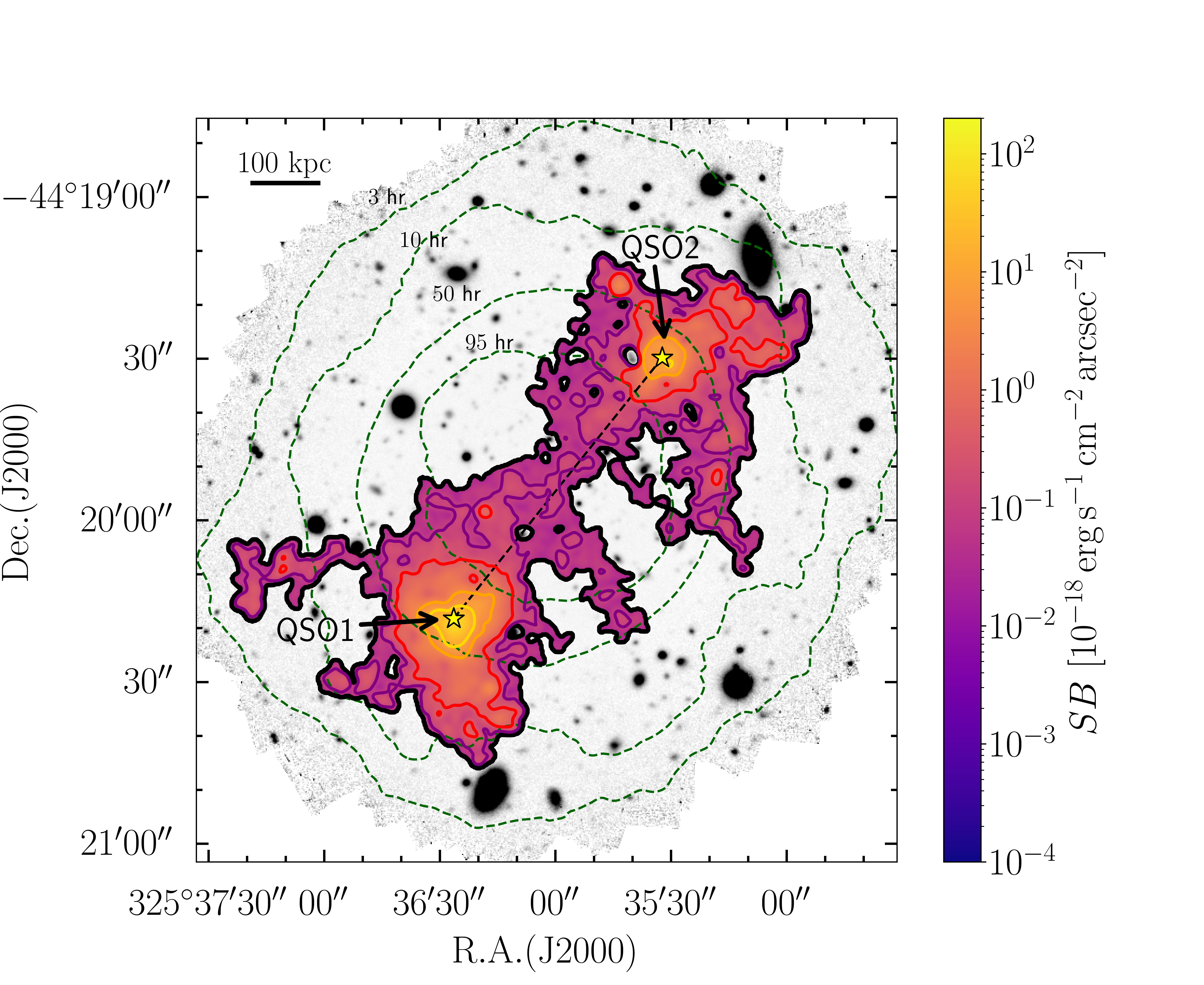
Figure 1: Optimally-extracted Ly$\alpha$ image of the extended nebulae surrounding the two quasars (marked by yellow stars and the respective labels QSO1 and QSO2) and of the filament connecting them along the diagonal direction (dashed black line, $\sim 500$ pkpc). The contour levels are $0.02$, $0.1$, $0.4$, $3.2$, and $10\times 10^{-18}$ erg s^-1 cm^-2 arcsec^-2  (black, purple, red, orange, and gold). The last black contour is the detection limit at $S/N=2$. The color bar covers the same values of Fig. 4. The background, in grey, is a white-light image of the region imaged by MUSE, with the dashed green contours defining the exposure time map of the field according to the labeled values.

Results

Detection and properties of the filament

Prior analysis of a partial-depth dataset of $\sim 40$ hr [15] uncovered extended Ly$\alpha$ nebulae in the circumgalactic medium (CGM) of the quasar hosts, with asymmetric extensions along the direction of the two active galactic nuclei. Based on these features that hinted at a gaseous bridge, we searched the region across the two quasars for low-surface brightness Ly$\alpha$ emission by selecting groups of connected pixels with signal-to-noise ($S/N$) above a threshold of 2 (see Supplementary Online Material, SOM, for further details). This exercise identified Ly$\alpha$ emission in a connected region occupying $\approx 30\times 90$ arcsec². Fig. 1 shows the optimally projected surface brightness map of the connected emission, along with labels for the two quasars, QSO1 (the brighter) and QSO2 (the fainter). Table 1 summarizes the main properties of the emitting structures that we describe next.

	Area	Mean Surface Brightness	Integrated flux	Size
	(arcsec2)	($10^{-19}$ erg s-1 cm-2 arcsec-2)	($10^{-16}$ erg s-1 cm-2)	(pkpc)
Nebula 1	$635^{*}$	$17.4\pm 0.1$	$11.1\pm 0.1^{*}$	117
Nebula 2	$530^{*}$	$7.1\pm 0.1$	$3.78\pm 0.05^{*}$	108
Filament	$830^{*}$	$0.81\pm 0.06$	$0.69\pm 0.05^{*}$	250

Table 1: Global Ly$\alpha$ properties of the two nebulae and the filament. The nebulae properties are computed using circular apertures up to the transition radius between CGM and IGM (see details in the text below) and centered on the quasar. This transition radius also defines the size of the nebulae. The properties of the filament are calculated using a box aperture positioned between the two nebulae, at a distance given by the transition radii. The length of this box defines the reported size of the filament. ^∗These quantities depend on the selected analysis region (see Fig. S2).

An extended emission structure stretches for over $\approx 700$ pkpc in projection, both in between and opposite directions of the two quasars. With a mean surface brightness of $\approx 8\times 10^{-20}$ erg s^-1 cm^-2 arcsec^-2, the filamentary structure between the two quasars would not have been detected in shallower data acquired by most surveys that reach $\gg 10^{-19}$ erg s^-1 cm^-2 arcsec^-2. The map also reveals smaller sub-structures that protrude from the main filament. While some sub-structures are likely affected by noise, especially in regions of moderate depth due to the non-uniform sensitivity of the map, the smaller filaments extending sideways from the central part of the main structure and the nebula of the QSO2 are likely real features, as also demonstrated by the spectra extracted in four different boxes positioned along the filament and near the QSO2 (see in SOM the Fig. S1). The overall morphology of the system, composed of galaxies, nebulae, and filaments, is remarkably similar to the configuration of galaxies assembling inside the cosmic web predicted by modern cosmological simulations [16, 17].

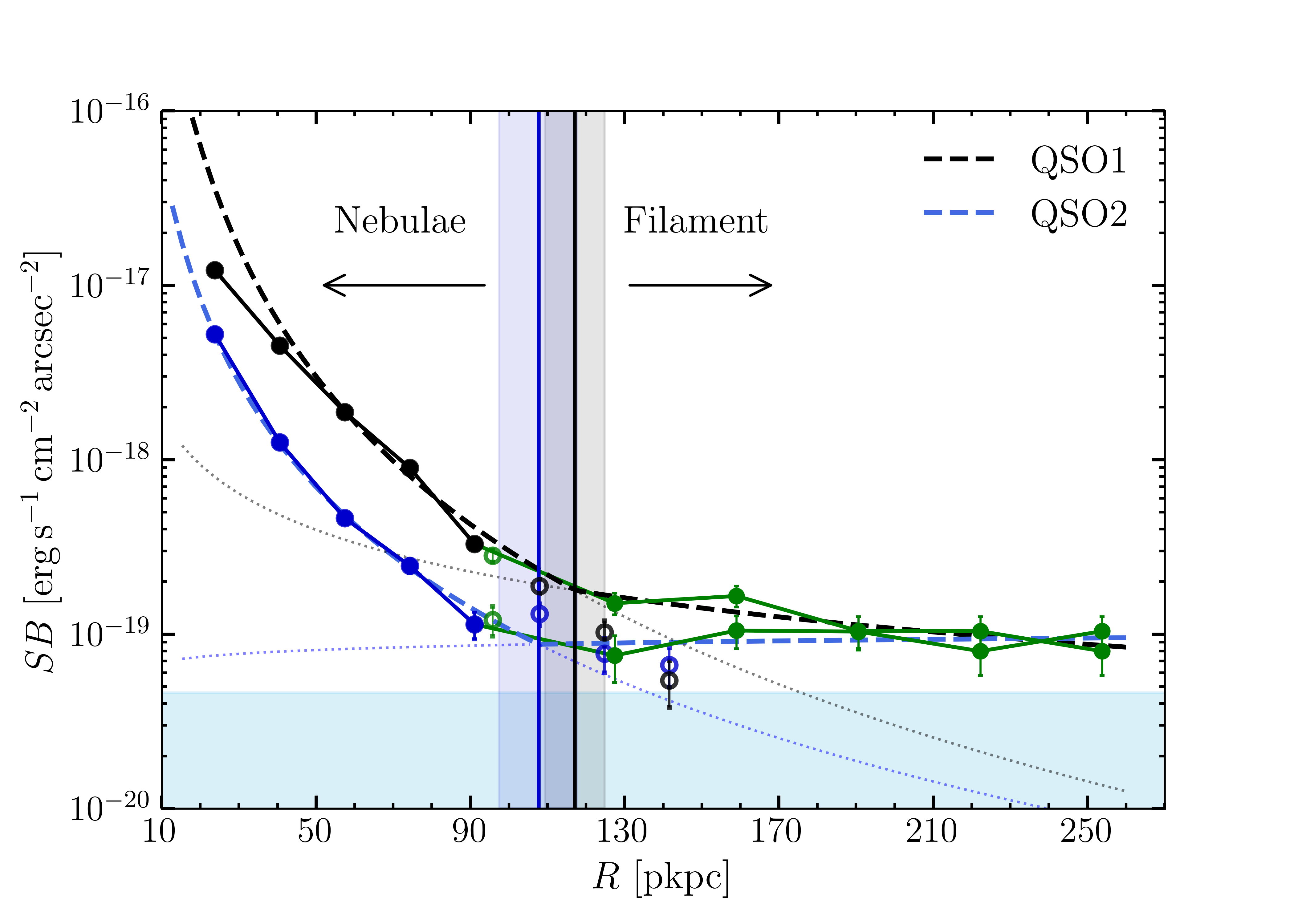
(a)

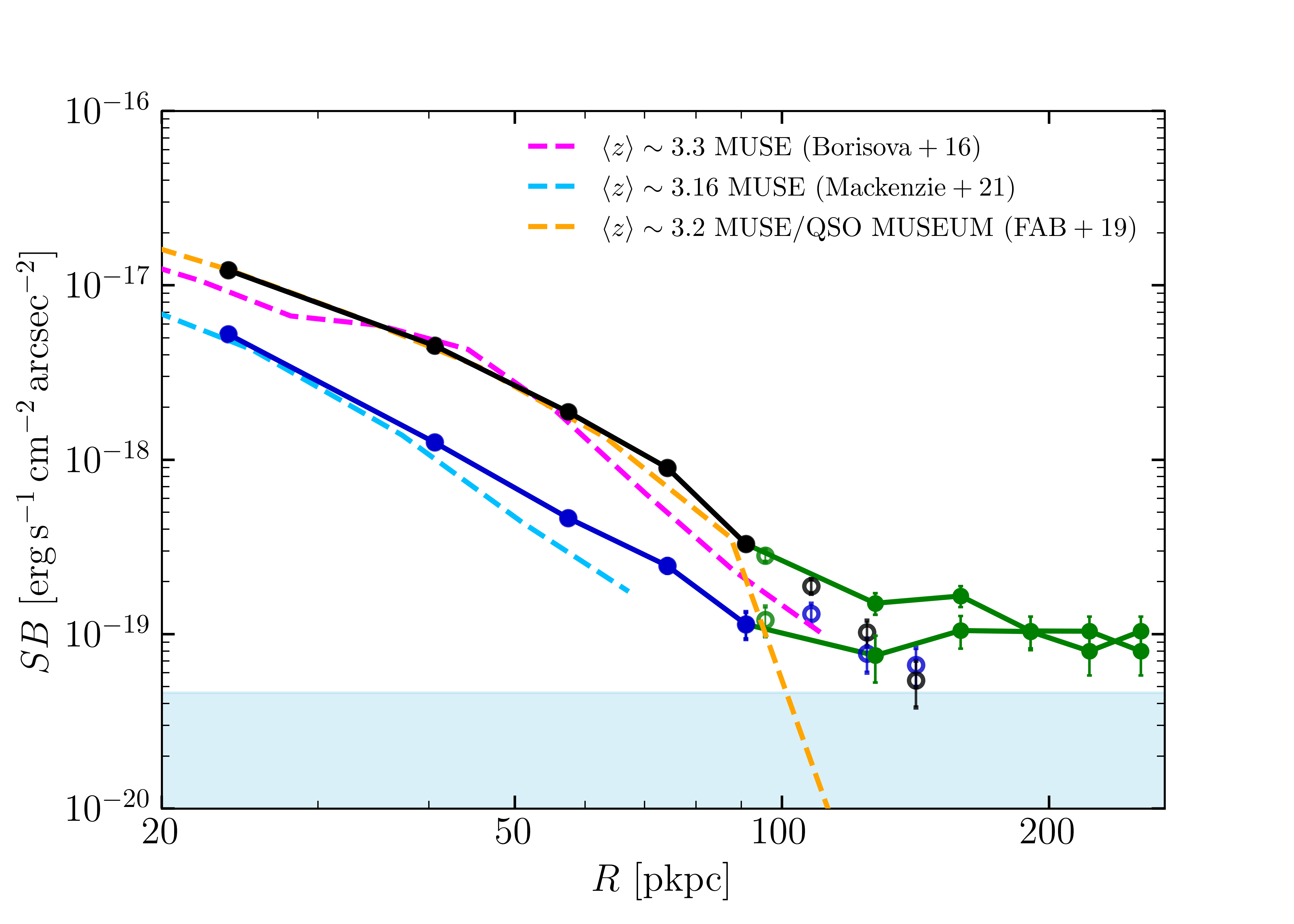
(b)

Figure 2: The complete Ly$\alpha$ surface brightness profiles of the nebulae and filament. (a) The extended Ly$\alpha$ emission’s surface brightness profile at the positions of QSO1 (black solid line) and QSO2 (blue solid line) are shown with filled dots, along with the filament profile (green solid line). The empty dots are the remaining data points measured using the different apertures (see SOM). The dashed lines (black and blue) represent the best-fit double power-law models. The two vertical solid lines (black and blue) denote the values with errors of the transition radii that separate the quasars’ CGM from the filament. The dotted black and blue lines represent the extrapolation of the single power laws of the fitted function. (b) Comparison between the measured surface brightness profiles in log-log scale and literature profiles (dashed lines) in statistical samples at comparable redshift and quasar magnitudes. In both figures, the horizontal sky-blue region marks the narrow-band detection limit at $4.5\times 10^{-20}$ erg s^-1 cm^-2 arcsec^-2  (see SOM for the definition).

The superb depth of the MUSE observations in the MUDF not only allows the detection of the low-surface brightness filament but also provides data of sufficient quality for an in-depth analysis of its structural properties. Such an analysis has never been performed to date. Furthermore, the presence of the bright quasars is likely boosting the emissivity of the denser gas near the host galaxies, as predicted by simulations [18] and seen in other environments populated by AGNs [8]. Starting with the flux-conserving projected surface brightness map obtained by collapsing the MUSE datacube in a wavelength window of $30$ Å centered on the expected Ly$\alpha$ emission peak at the redshift of the two quasars, we extract the Ly$\alpha$ surface brightness profile along the axis connecting the two quasars. We adopt a circular geometry and derive the azimuthally average profile for the emission arising in the nebula near the quasars. For the filament emission, we extract instead the average surface brightness along the axis connecting the quasars inside rectangular regions (see Fig. S2 in the SOM for details). The central region within $\approx 15$ kpc of each quasar is excluded from the analysis due to the residual of the quasar point spread functions, which have been subtracted from the original cube. The emission extracted from the nebulae and the filament profile join smoothly, and we use the radius at which they intersect to switch from one geometry to another (see SOM for a detailed explanation).

The resulting profiles are shown in Fig. 2(a) on a linear scale and in Fig. 2(b) on a logarithmic scale to better highlight the inner radii dominated by the quasar nebular emission. Upon inspection of these figures, we see that the profiles rapidly decline with radius, following a power law with index $\approx-3.3$ for Nebula 1 and $\approx-2.7$ for Nebula 2 (see SOM for details on the fitting procedure), before reaching a plateau of almost constant surface brightness in the region dominated by the filament emission. The profile near QSO2 appears to be a scaled-down version of that centered on QSO1. As the bottom panel of this figure shows, the radial profile measured for the two nebulae is very consistent in shape and normalization with the average profiles obtained for bright and faint quasar samples [19, 20, 21]. Hence, the MUDF quasar nebulae are not outliers but typical under this metric.

Following the observed surface brightness profiles to larger radii makes a slope change apparent at $\lesssim 10^{-19}$ erg s^-1 cm^-2 arcsec^-2. We attribute this variation in the power law index to the transition between the regime dominated by the CGM of the quasar host galaxies and the IGM. This is similar to the analysis performed in a nearby galaxy by Nielsen et al. [22] to infer the transition between the interstellar and circumgalactic medium. By modeling the full profile with a double power-law profile (see Equation 1 in the SOM), we constrain the transition radius between these two regions, $R_{t}$. For QSO1, $R_{t}=117\pm 8$ pkpc, while for the fainter quasar QSO2 $R_{t}=107\pm 10$ pkpc. Values of $\approx 100$ pkpc are comparable to the virial radius of halos with mass $\approx 2-3\times 10^{12}$ M_⊙, which is the estimated halo mass of $z\approx 3$ quasars at these luminosites [23], [24]. This analysis, therefore, provides one of the very few examples currently available in which the transition radius between the CGM and IGM is directly measured, and the only such measurement in emission at cosmic noon. For comparison, at lower redshift ($z<0.5$), using absorption line statistics and by measuring the covering fraction of H I absorption, Wilde et al. [25] found a typical size of about twice the virial radius for the CGM of star-forming galaxies.

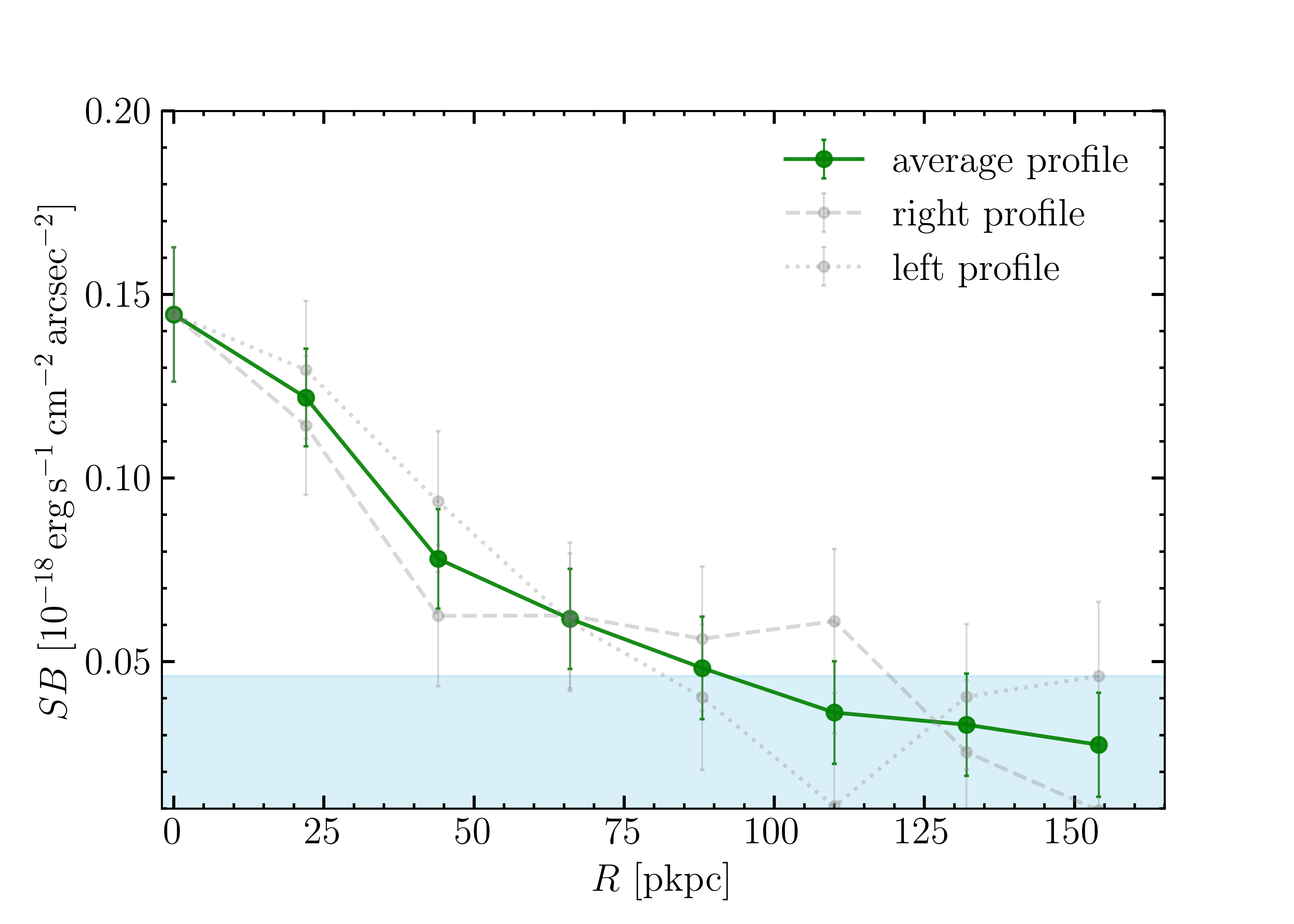
Figure 3: The transverse Ly$\alpha$ surface brightness profile of the filament. The dashed and dotted grey lines represent the right and left profiles relative to the direction connecting QSO1 with QSO2. The green solid line shows the resulting average profile combining the two. The horizontal sky-blue region marks the narrow band detection limit at $4.5\times 10^{-20}$ erg s^-1 cm^-2 arcsec^-2(see SOM for the definition).

The unique nature of the MUDF system further allows for the measurement of the filament properties in the direction transverse to that connecting the quasars (i.e., the spine). For this analysis, we employ again rectangular extraction boxes in the region outside the quasar CGM ($R>R_{t}$) and measure the average surface brightness profile on both sides of the filament’s spine (see Fig. S2 in the SOM). Both sides yield a comparable measure that we average to construct a final transverse Ly$\alpha$ profile (Fig. 3). In the transverse direction, the profile drops with a power law index of $\approx-0.74$ up to $\approx 70$ pkpc. The total thickness is $\lesssim 2\times 70\approx 140$ pkpc at the depth of our observations, reaching the detection limit of the narrow band image, estimated as $4.5\times 10^{-20}$ erg s^-1 cm^-2 arcsec^-2. The increased noise level likely contributes to the flattening at larger radii ($\approx 100$ pkpc). Hence, there is no strong evidence in current data of an edge or change of slope in the profile.

The MUDF filament in cosmological context

To generalize the properties derived from the MUDF filament to other cosmic environments, we assess how typical this double-quasar system is expected to be in our Universe. For this task, we search for MUDF twins in the semianalytic model (SAM) L-Galaxies based on the Millennium simulation [26, 27] (see SOM for further details). We opt for this model as it implements detailed quasar physics that successfully reproduces key statistics of the quasar population, including the observed luminosity function. By selecting simulated quasar pairs within 0.3 dex of the observed bolometric luminosities [28] with projected distances of $400-600$ pkpc and line-of-sight velocity separation of $\Delta v\leq 1000$ km s^-1 (as estimated from the redshift of the quasars, see SOM), we find that the three-dimensional physical distance of pairs is closer than 2.5 pMpc for 95% of the systems, and less than 1 pMpc in half of the cases (see Fig. S4). We thus conclude that filamentary structures similar to that connecting two MUDF quasars are not unlikely to occur within a $\Lambda$CDM universe.

With this SAM, we also infer a number density of quasar pairs of $5.6\times 10^{-9}$ cMpc^-3, implying an expected occurrence of one MUDF-like quasar pair within a random volume of ($560$ cMpc)³. Using these twins, we derive the distribution of halo masses of the bright and faint quasars (see Fig. S3), from which we infer a typical halo mass of $\log(M_{\mathrm{vir}}/M_{\odot})=12.91^{+0.34}_{-0.33}$ for the brighter quasar and $\log(M_{\mathrm{vir}}/M_{\odot})=12.25^{+0.46}_{-0.35}$ for the fainter one. These values are in line with current estimates at comparable redshifts [23, 24]. As we have no reason to expect that the underlying density distribution within the filament depends on the presence of quasars, we can use the halo mass distributions obtained from the SAM to select pairs of halos with separations of $\lesssim 1$ pMpc to investigate further the physical properties of filaments inside cosmological hydrodynamic simulations.

For this analysis, we use the intermediate-resolution simulation box publicly available from the IllustrisTNG project (TNG100$-$1, see SOM; [29]), representing a compromise between resolution and volume. Within this box, we identified 144 pairs with halo masses based on the distribution obtained from the SAM, with a projected distance in the range of $400-600$ pkpc and a 3D distance below $1$ pMpc. First, we confirm that these pairs are generally physically connected by a dense filamentary structure in contrast to pairs that have larger physical distances, $>2$ pMpc, as also inferred from the SAM (see Fig. S4). A thorough inspection of the simulated pairs reveals that the median density profile along the direction that connects the two halos (see SOM) declines from the central regions smoothly reaching a plateau with a minimum value of $\sim 10^{-3.7}$ cm^-3, i.e., approximately ten times the average cosmic density at these redshifts ($\approx 1.4\times 10^{-5}$ cm^-3). In contrast, for pairs with a physical distance $>2$ pMpc, the minimum value of the median profile reaches $\sim 10^{-4.8}$ cm^-3 (see Fig. S5), not far from the mean density. Along the filament’s axis for connected pairs, the hydrogen density reaches a median peak value of $10^{-2.8}$ cm^-3 (see the transverse profile in Fig. S6), indicating the presence of a denser spine in the central part of the cosmic web.

Figure 4: Example of a simulated pair with a 3D physical distance below 1 pMpc, closely resembling the MUDF system. The left panel shows the hydrogen column density map, and the central panel displays the surface brightness map, smoothed on the same scale as the reconstructed MUDF maps. Contour levels of $10^{-20}$, $10^{-19}$, and $10^{-18}$ erg s^-1 cm^-2 arcsec^-2 are marked (black, red, and light-yellow lines). Right panel: the transverse surface brightness profile of the MUDF twin (black line) compared to the MUDF data (red line). Also shown is the median transverse profile obtained with the pairs with a 3D distance below 1 pMpc (yellow line with shaded regions marking the $16^{\rm th}$ and $84^{\rm th}$ percentiles). The profile is shown up to $\sim 70$ pkpc, where the measurements exceed the detection limit.

As two of the main Ly$\alpha$ emission mechanisms (recombination radiation and collisional excitation) depend quadratically on density, a comparison between the observed and predicted surface brightness of filaments offers a novel way to constrain the typical order-of-magnitude underlying gas density within the filaments. We compute surface brightness maps (see a full description in SOM) under the approximation where recombinations and collisional excitations give the total emissivity of the diffuse gas, i.e., below the densities at which the gas in the adopted model lies on the imposed equation of state ($n_{H}<0.1~{}\rm cm^{-3}$). Due to the presence of the quasars, we also consider a maximal fluorescence model, where the bright sources fully ionize the gas that emits only through recombination. As the adopted simulation may not fully resolve the gas density distribution, which is a key ingredient that modulates the observed surface brightness, we also study the resolution effects by repeating the same analysis in other boxes of the TNG suite across a factor of $\sim 200$ in resolution (see SOM). Following the same methodology adopted in the analysis of MUDF data, we calculate the median transverse surface brightness profile of the filaments between the pairs (Fig. S7). The predicted surface brightness is generally insensitive to the details of the assumed emission mechanisms and the resolution adopted for the simulations.

The observed and simulated profiles share a different normalization. However, raising the filaments’ density by less than a factor of three would be enough to match the observed profile, considering the contribution of recombinations alone. A further contribution from collisions reduces this discrepancy, which could even be removed if $n_{H}>0.1~{}\rm cm^{-3}$ gas is considered (see SOM). Furthermore, our simple model does not include scattering, which detailed radiative transfer calculations indicate as an important contribution to the observed signal [30]. Finally, owing to the scatter of the various simulated profiles, we can identify close matches in terms of the transverse surface brightness profile of the MUDF filament inside this simulation. One such example is in Fig. 4.

From this comparison, we conclude that the typical density inferred from the cosmic web in these simulations must be of the order of what is found in the MUDF filament, and, at present, there are no obvious indications of tensions between observations and the predictions of the cosmic web in the adopted cold dark matter model. Our study, which has offered the first quantitative measurements of the structural properties of the cosmic filaments at cosmic noon beyond a simple detection, provides a tantalizing novel avenue for constraining with quantitative data the cosmic web, which is one of the fundamental predictions of cold dark matter.

Conclusions

The unprecedented depth, with a detection limit in the narrow-band image of $4.5\times 10^{-20}$ erg s^-1 cm^-2 arcsec^-2  reached by the MUDF observations in a double-quasar field has enabled the detection of a prominent cosmic filament connecting two quasar-host halos at $z\sim 3.22$. These observations represent the highest-definition view of the cosmic web to date, allowing us to characterize the filament morphology and directly measure for the first time the transition radius between the IGM and the CGM, which occurs around the virial radius for $\approx 2-8\times 10^{12}~{}$M_⊙ halos. We also derived the surface brightness profile along the filament and in the transverse direction. With the aid of SAM and cosmological hydrodynamical simulations, we have shown how the MUDF field, although special for the exceptional dataset, is an excellent laboratory to study the physics of filaments connecting $\gtrsim 10^{12}-10^{13}~{}$M_⊙ halos at cosmic noon. Our analysis reveals that a main filament, with gas overdensities above ten times the mean cosmic density, connects most halos with physical separation $<1$ pMpc. This differs from what is seen in pairs at larger separations, e.g., $>2$ pMpc, where the gas between halos drops to the mean density.

By exploiting the quadratic dependence of the Ly$\alpha$ emissivity for two main channels of photon production, recombination and collisional excitation, we have used the observed surface brightness maps to test the predicted density distribution of cosmic filaments in the current cold dark matter model. We found a shift between the simulated and observed Ly$\alpha$ surface brightness levels. However, this difference can easily be removed by raising the underlying density of the filaments by less than a factor of three, demonstrating that the typical densities in models are within acceptable values. Moreover, we identified examples inside the simulation that closely match the observed MUDF system. Therefore, the current data do not highlight significant tensions with the cold dark matter model. By moving from detections to quantitative analysis of the cosmic web, our study demonstrates the exciting potential of spectrophotometry of cosmic filaments for testing how cosmic structure proceeds. Our pathfinder study opens the way to quantitatively characterize the structure and physical properties of the cosmic web, which is a fundamental prediction of the current cosmological model and - also thanks to its simpler gas physics compared to the galaxies - should be explored more as a way also to test the essence of dark matter. Building on our work, future ultradeep observations of cosmic filaments in the era of 40m telescopes coupled with sophisticated numerical models will strengthen our understanding of the Universe in novel ways.

Author contributions DT analyzed the observations and was the main author of the manuscript. MiFu coordinated the MUDF program, participated in the data analysis, and co-authored the manuscript. MaFo reduced and analyzed the observations and participated in the analysis and manuscript writing. ABL contributed to the simulation analysis and DIV created and provided the SAM lightcone, and contributed to the analysis. All co-authors participated in preparing the manuscript. Acknowledgments This project has received funding from the European Research Council (ERC) under the European Union’s Horizon 2020 research and innovation program (grant agreement No 757535 and No 101026328), by Fondazione Cariplo (grant No 2018-2329) and is supported by the Italian Ministry for Universities and Research (MUR) program “Dipartimenti di Eccellenza 2023-2027”, within the framework of the activities of the Centro Bicocca di Cosmologia Quantitativa (BiCoQ).

Supplementary Materials

Materials and Methods
Figs. S1–S7
References (31-41)

Materials and Methods

Observations and data reduction

Observations of the MUSE Ultra Deep Field ($\mathrm{R.A.}=21^{h}$:42^m:24^s, $\mathrm{Dec.}=-$44^∘:19^m:48^s) have been obtained as part of the ESO Large Programme (PID 1100.A$-$0528; PI Fumagalli) between periods 99-109, using the MUSE instrument in wide-field mode with extended wavelength coverage between $\lambda 4650-9300$ Å. A total of 142.8 h on-source have been collected with multiple exposures through a dither pattern and field rotations designed to cover an $\approx 1.5\times 1.5$ arcmin² area, with maximal sensitivity in the inner $\approx 1$ arcmin² region (see Fig. 1). Using the GALACSI adaptive optics system improves the image quality compared to natural seeing, yielding a full width at half-maximum of $\approx 0.73$ arcsec for point sources.

Using standard techniques from the MUSE pipeline [v2.8 31], we corrected the raw data for primary calibrations (bias, dark, flat correction, and wavelength and flux calibration). Next, individual exposures, sky-subtracted and corrected for residual illumination using the CubExtractor toolkit (v1.8, CubEx hereafter, see [32] for further details), are coadded in a final datacube with a pixel size of $0.2$ arcsec and $1.25$ Å in the spatial and spectral direction, respectively. An associated variance cube is also reconstructed through the bootstrap technique we developed in previous work [33], [14]. The final data achieve a pixel root-mean-square (rms) of $3\times 10^{-21}$ erg s^-1 cm^-2 Å^-1 pix^-1 (at $\sim 5200$ Å, see below), making this the deepest MUSE observation to date, en pair with the MUSE eXtreme Deep Field, which reached comparable limiting fluxes [9].

Due to the exquisite sensitivity of these data and the fact that we are interested in extended low surface brightness emission, we minimize the impact of small sky residuals by performing a final correction of the background level. For this, we select pixels in regions empty of continuum sources and far from where we expect Ly$\alpha$ emission. After identifying the extended emitting structure in the datacube (see next section), we explicitly check that no source contribution is contained in these sky regions. We next construct a median sky spectrum over $\approx 5000$ pixels and use this spectral template for the final sky subtraction. Locally, this template is normalized to the residual sky values measured in two narrow-band (NB) images of spectral width $60$ Å, which we select around $\lambda=4800$ Å, and $\lambda=5400$ Å, i.e., far enough from the wavelength interval where we expect Ly$\alpha$ emission from $z\approx 3.22$ sources. Ultimately, we achieve a robust sky subtraction, where the residual level is $<1\%$ of the pixel rms measured in the deepest central region of the field of view ($>95~{}\rm hr$) and in the spectral range (4900-5100 Å) and (5200-5400 Å) that is adjacent to the wavelengths where we expect Ly$\alpha$ emission.

Identification and extraction of the filament and nebulae

The presence of two bright Ly$\alpha$ emitting nebulae around the two MUDF quasars was already confirmed in a partial, $\approx 40$ hour dataset by Lusso et al. [15]. To search for more extended and very low-surface brightness emission in the datacube, we use the CubEx tool to subtract continuum-emission sources and the quasar point spread function through a nonparametric continuum-subtraction algorithm (see [32] for further details). Next, we identify groups of $>2500$ connected voxels above a signal-to-noise ($S/N$) threshold of 2, with a minimum number of $500$ spatial pixels. To increase the sensitivity to low-surface brightness emission, we further smooth the cube with a Gaussian kernel with a size of $3$ pixels ($0.6$ arcsec or $4.6$ pkpc) in the spatial direction, masking continuum sources to avoid contamination from negative or positive residuals created during the continuum subtraction process. No smoothing is applied in the wavelength direction to maximize the spectral resolution. We also demand that at least $3$ wavelength layers be connected in the spectral direction to avoid spurious thin sheets of emission.

This search yields two connected and very extended structures ($>30000$ voxels). One of them covers the two quasars, with the brightest emission coinciding with the quasar positions. The other one is the already identified Nebula 3 by Lusso et al. [15]. The quasars Ly$\alpha$ nebulae are detected to a surface brightness limit of $\sim 1\times 10^{-19}$ erg s^-1 cm^-2 arcsec^-2  in the new data. With the ultradeep observations in the central region, we also uncover a filamentary and extended emission signal that originates from the edges of the quasar nebulae and connects them in the direction of the putative filament proposed by Lusso et al. [15]. Additional extended emission is detected in the opposite direction for both quasars, suggesting that the emitting structure extends for more considerable distances than probed by our data. The detection of the nebulae and the filament with their overall morphology does not depend on the selection criteria described above. Indeed, we perform the extraction using different $S/N$ thresholds (up to 2.5) and different spatial (2 and 4 pixels) and spectral (0 and 1 pixel) smoothing settings, all of which yield the same global emission structures, once considered the different parameters employed. The detected signal is then projected along the wavelength direction to compose an optimally extracted Ly$\alpha$ image, shown on the top of the white-light image in Fig. 1 and in Fig. S1 on the top of three collapsed wavelength layers at the central wavelengths of the nebulae to assess the background noise level. Optimally-extracted maps are best suited to highlight low surface brightness emissions. Still, as it combines only the voxels identified by CubEx above the $S/N$ threshold as harboring significant emission, it may lose flux and is insufficient for precise estimates of the total surface brightness (see, e.g., [19]). Therefore, we resort to a synthesized NB image centered on the expected Ly$\alpha$ emission peak and obtained by summing the flux in the wavelength direction over $30$ Å for all the measurements presented in this work.

While the nebulae are detected at high $S/N$, the extended low-surface brightness signal across the filament, with $\approx 8\times 10^{-20}$ erg s^-1 cm^-2 arcsec^-2, is close to the detection limit of the NB image ($\approx 2\sigma$, see below how $\sigma$ is defined in the NB image). Therefore, we perform a series of tests to confirm the genuine nature of the detection. Firstly, we search again for the detected signal in a primary data reduction before applying any illumination correction or enhanced sky subtraction using the CubEx code. Secondly, we verify the presence of the extended structure in two independent coadds containing each half of the total number of exposures. The filament is recovered in each test, although at lower $S/N$ due to the higher noise of the various products and methods used for this test. Finally, we verify that the signal is a significant spectral feature in the datacube. We extract spectra from four distinct boxes, denoted as A, B, C, and D, each $\approx 14\times 8$ arcsec² and positioned along the main filament and in the vicinity of the QSO2, as illustrated in the top panel of Fig. S1. In the bottom panel of Fig. S1, we present the extracted normalized spectra for each extraction box. The spectra are shown in velocity space, with the reference zero velocity (marked by the vertical dashed blue line) calculated from the first moment of the line within a wavelength range $\pm 10$ Å around the expected emission peak. The dashed horizontal green line represents the 1$\sigma$ noise level of the spectrum estimated from all the wavelengths not in the interval of the Ly$\alpha$ emission. The spectra extracted in these regions confirm that the detected signal is an actual emission of astrophysical origin and does not arise from spurious noise or systematic artifacts in the advanced processing of the data. Due to the faint nature of the signal, however, we caution that the detailed small-scale morphology visible in Fig. 1 as thin protuberances from the main filament is more affected by noise and not very robust.

Figure S1: (Top panel) Optimally extracted Ly$\alpha$ image on top of three collapsed wavelength layers at the central wavelength of the quasar nebula emission. The contour levels are $0.02,0.06,0.3$ and $2\times 10^{-18}$ erg s^-1 cm^-2 arcsec^-2 (light-grey, black, light-orange, purple). (Bottom panel) Normalized spectra in velocity space extracted from the white boxes labeled A, B, C, and D in the top panel. The vertical dashed blue line represents the zero velocity reference calculated from the first moment of the line, and the horizontal dashed green line represents the $1\sigma$ noise level of the spectrum.

Analysis of the surface brightness profiles

We compute the surface brightness profiles of the nebulae associated with the two quasars and the filament from the synthesized NB image. Before extracting the surface brightness profiles, we apply a mask to avoid residuals of the continuum subtraction of compact sources, which could introduce contamination. Nevertheless, the percentage of unmasked pixels in each region used for the analysis is $>80$ percent. Subsequently, for each nebula, we compute the circularly averaged surface brightness profile, using rings with an aperture of $\approx 10$ spatial pixels (equivalent to $\approx 2$ arcsec, or $\approx 15$ pkpc), up to a radius of 150 pkpc centered at the positions of the quasars. Hereafter, we will use the term Nebula 1 (Nebula 2) to refer to the one associated with the brighter (fainter) quasar, QSO1 (QSO2), as indicated in the left panel of Fig. S2. In Fig. S2, we overplot the annuli on the optimally extracted image within which we calculate the surface brightness profiles, in black for Nebula 1 and blue for Nebula 2. We exclude a circular $2$ arcsec² region around the quasars to avoid residuals from the point spread function subtraction (the two black dots). Hence, the radial profiles are presented for $R\gtrsim 15$ pkpc. Instead, we employ ten boxes for the filament, each with dimensions of approximately $20\times 80$ pixels² along the direction connecting the two quasars, starting at a distance of $80$ pkpc from them. These boxes are in green in the left panel of Fig. S2.

Figure S2: (Left panel) Extraction apertures (black annuli for Nebula 1, blue annuli for Nebula 2, and green boxes for the filament) used to extract the surface brightness profiles, superimposed to the Ly$\alpha$ emission map. The two black dots mark a $\approx 15$ pkpc radius where the quasar’s PSF residuals dominate the signal. QSO1 and QSO2 are indicated by the two black arrows, respectively. (Right panel) Same as panel (a) but for the transverse surface brightness profile. In the background of both images, in grey, is a white-light image of the region imaged by MUSE.

To calculate the surface brightness value for each annulus and box, we adopt a weighted average of all the unmasked pixels, consistently propagating the errors from the associated variance image. Considering the varying aperture widths and shapes used and the irregular geometry of the emission, we examine the overlapping regions between the rings and the boxes to join the nebula and the filament profile. In Fig. 2(a), the observed surface brightness data points are shown using the same colors as for the extraction apertures in the left panel of Fig. S2: black dots represent the measured values in the annuli for Nebula 1, blue dots represent those for Nebula 2, and green dots represent those for the boxes in the filament. The filled dots mark the combined surface brightness profiles, while the empty dots are the individual aperture measurements not included in the final profile and up to the detection limit of the NB image.

The profile from both quasars is rapidly declining to $\approx 100$ pkpc scales, which we identify as the Ly$\alpha$ nebulae arising from the host circumgalactic medium (CGM). The plateau at $\gtrsim 100$ pkpc extending to $250$ pkpc – the midpoint between the two quasars – is instead arising from the filament. Examining the empty data points of the two nebulae above $\sim 100$ pkpc, the excess emission from the filament becomes evident compared to what is measured in the annuli. Clearly, the filament signal is also enclosed in the annuli, but the filling factor becomes progressively low for increasing radius, making this circular geometry a poor choice for the filament surface brightness. Moreover, the annuli include the signal on the opposite side of the nebulae, where the filamentary structure is fainter, yielding a steeper profile.

Examining the two nebulae, in Fig. 2(b), we compare the observed profiles on a log-log scale with the average profile from the $z\sim 3.3$ sample of Borisova et al. [19] (dashed magenta line), the $z\sim 3.2$ sample of Arrigoni Battaia et al. [20] (dashed blue line) and the $z\sim 3.16$ faint sample of Mackenzie et al. [21] (dashed sky blue line). We observe that both our nebulae have a profile that is in excellent agreement with those in literature at the same redshift, once accounting for the different magnitudes of each quasar. Indeed, the $i-$band magnitudes of the quasars in the sample from Borisova et al. [19] range from $16.6$ mag to $18.6$ mag. Those from Arrigoni Battaia et al. [20] range from $17.4$ mag to $19$ mag and include in the sample the brighter QSO1, with a $i-$band magnitude of $17.6$ mag. Finally, the $i-$band magnitude of the quasars in Mackenzie et al. [21] ranges from $20$ mag to $23$ mag, thus being comparable to the fainter QSO2, with a magnitude of $20.6$ mag in the same band. This comparison concludes that both quasars have a typical CGM when traced by Ly$\alpha$ despite being in a close-separation pair.

An evident inflection point is visible in both profiles around $\approx 100$ pkpc from the quasars, which we ascribe to the transition between the CGM traced by the quasar’s nebulae and the IGM traced by the filament. To explore this transition more and to separate the emission of these two components, we fit the complete surface brightness profiles (filled dots) with the following broken power law model

$$SB(R;A,R_{\mathrm{t}},b_{1},b_{2})=\begin{cases}A\left(\frac{R}{R_{\mathrm{t}}}\right)^{b_{1}},&\text{if }R\leq R_{\mathrm{t}},\\ A\left(\frac{R}{R_{\mathrm{t}}}\right)^{b_{2}},&\text{if }R>R_{\mathrm{t}}.\end{cases}$$ (1)

$R_{\mathrm{t}}$ is the transition radius between the CGM and the IGM, $A$ is the normalization, and $b_{1}$ and $b_{2}$ are the two slopes. The choice of a power law function is justified in the quasar Ly$\alpha$ nebulae literature context (e.g., [19], [20]). To determine the best parameters, we employ a Bayesian approach: we assume a Gaussian likelihood for each surface brightness estimate, where $SB(R)\sim\mathcal{N}(SB(R;A,b_{1},b_{2}),\sigma_{\mathrm{SB}})$, with $\sigma_{\mathrm{SB}}$ representing the propagated error. Additionally, we apply a uniform prior on the model parameters in the following intervals: $[60,180]$ pkpc for $R_{\mathrm{t}}$, $[0,1]$ erg s^-1 cm^-2 arcsec^-2  for $A$, $[-4,-1]$ for $b_{1}$, and $[-2,2]$ for $b_{2}$. The best-fitting parameters for the surface brightness profile associated with quasar 1 are $R_{\mathrm{t}}=117\pm 8$ pkpc, $A=0.18\pm 0.04$ erg s^-1 cm^-2 arcsec^-2, $b_{1}=-3.3\pm 0.1$, and $b_{2}=-0.9\pm 0.3$. For quasar 2, the best parameters are $R_{\mathrm{t}}=108\pm 10$ pkpc, $A=0.09\pm 0.03$ erg s^-1 cm^-2 arcsec^-2, $b_{1}=-2.71\pm 0.03$, and $b_{2}=0.1\pm 0.4$. The best fits are shown in Fig. 2(a) as black and blue dashed lines for QSO1 and QSO2. The solid vertical lines, with the same colors, represent the transition radius and its error. Instead, the dotted black and blue lines represent the extrapolation of the best fit for the nebulae and the filament for each quasar, further confirming the presence of an emission excess in the filament region. This model thus recovers a natural transition between the CGM and IGM in the range of $\approx 90-130$ kpc, with the fainter quasar having a smaller size of the Ly$\alpha$-emitting CGM as observed in previous studies ([21],[34]). For typical halo masses in the order of $\approx 10^{12.3-12.5}$ M_⊙ for these quasars ([23], [24]), the virial radius at $z\approx 3.2$ is $R_{\rm vir}=92-108$ kpc, i.e., comparable with the size of the transition radius. The transition occurs at a surface brightness of $\approx(1-2)\times 10^{-19}$ erg s^-1 cm^-2 arcsec^-2, with only a small difference with the quasar luminosity.

The depth and quality of the data also allow us to extract the transverse surface brightness profile of the filament. We calculate the weighted average value from boxes measuring $\approx 160\times 14$ pixels² each, up to a distance of $165$ pkpc on both the right and left sides relative to the direction connecting the two quasars. The 15 boxes are off-axis by 7 pixels in the NW direction to achieve the emission peak in $R=0$. To account only for the filament emission, avoiding contamination from the two nebulae, the length of each box is determined by the distance from the two quasars, selected as the transition radius estimated above (see Fig. S2). The right and left surface brightness profiles are shown in Fig. 3 with grey dashed and dotted lines, respectively. A solid green line shows the combined average profile. Fitting the profile in the region above the detection limit with a power law, we obtain a slope of $-0.74\pm 0.15$, and we observe that the transverse projected width of the filament extends up to approximately $70$ pkpc at the depths of our observations. This value is similar to the shock radius found in Lu et al. [35] in simulations of filaments around a pair of two massive halos ($M\sim 5\times 10^{12}~{}M_{\odot}$), separated by a distance of $1.2$ pMpc at $z\sim 4$.

As the formal error does not fully account for the pixel covariance arising from the cube reconstructions [14], we calculate an empirical surface brightness detection limit in the central region of the field of view, specifically in the area with the deepest data ($>95$ hr) where the filament is detected. For this purpose, we extract an NB image of 30 Å, shifted by approximately 60 Å from the Ly$\alpha$ peak emission. This spectral region is chosen where we do not expect any source emission. We obtain the distribution of SB values by calculating the average along 1000 apertures of the box used to evaluate the filament profile, with size $20\times 80$ pixels², again masking any residuals of the continuum subtraction of compact sources. These apertures are randomly located in the central region of the field of view. The NB detection limit ($1\sigma$) is then determined as one the standard deviation of the distribution above the mean value. The resulting value is $4.5\times 10^{-20}$ erg s^-1 cm^-2 arcsec^-2, shown by the sky blue region in Fig. 2 and Fig. 3.

To measure the global properties of the detected emissions, we use the transition radius as a reference to differentiate between the nebulae and the filament. The nebula around QSO1 has a total flux of approximately $1.1\times 10^{-15}$ erg s^-1 cm^-2 over a total area of approximately $635$ arcsec², while the nebula around QSO2 has a total flux of approximately $3.8\times 10^{-16}$ erg s^-1 cm^-2 over a total area of approximately $530$ arcsec². This leads to a total luminosity of $\sim 1\times 10^{44}$ erg s^-1 for Nebula 1 and $3.6\times 10^{43}$ erg s^-1 for Nebula 2. The filament, considered up to approximately $70$ pkpc in the transverse direction, has an average surface brightness of approximately $8.3\times 10^{-20}$ erg s^-1 cm^-2 arcsec^-2. The total linear extension of the emitting structures is also computed by considering the projected distance between the two quasars and the projected distance up to $\sim 1\times 10^{-19}$ erg s^-1 cm^-2 arcsec^-2  on the opposite side of the filament, leading to $\sim 700$ pkpc. Table 1 summarizes these global properties.

Analysis of the semi-analytic model

We turn to the analysis of semi-analytical models (SAM) with two objectives: to place our system in a broader cosmological context by assessing the expected number density of these pairs and to infer the most probable distributions of dark matter halo masses of the MUDF quasars. For these tasks, we use a lightcone generated with the updated version of the L-Galaxies SAM models [36], as detailed in Izquierdo-Villalba et al. [26], [27]. These models are run using the sub-halo merger trees from the Millennium [37] dark matter N-body simulation within a periodic cube of side $500$ cMpc/$h$. The quasar phase of a galaxy is triggered by gas accretion onto black holes, and this model accounts in detail for these processes, reproducing statistics in good agreement with observations, including a quasar luminosity function (see Izquierdo-Villalba et al. [27] for a more comprehensive discussion). Therefore, we can leverage these models to identify systems similar to the MUDF.

By using the methodology presented in Izquierdo-Villalba et al. [26], we have created a lightcone covering the full sky in the redshift range $z\sim 2.8-3.8$, which is centered on the mean redshift of the two MUDF quasars ($z\sim 3.22$) and has a half width of $\sim 340$ Myr. Next, we select the bright quasars corresponding to QSO1 with a bolometric luminosity of $\log(L_{\mathrm{bol}}/L_{\odot})=47.3\pm 0.3$ and the faint sources corresponding to QSO2 with luminosity $\log(L_{\mathrm{bol}}/L_{\odot})=46.3\pm 0.3$ [28]. This results in a number density of approximately $3\times 10^{-7}$ cMpc^-3 and $8\times 10^{-6}$ cMpc^-3, respectively. The virial mass distribution for the two samples has a mean value of $\log(M_{\mathrm{vir}}/M_{\odot})=12.79^{+0.34}_{-0.32}$ for the bright sample and $\log(M_{\mathrm{vir}}/M_{\odot})=12.20^{+0.40}_{-0.30}$ for the faint one. The errors represent the $16^{\rm th}$ and $84^{\rm th}$ percentiles of the distributions. These frequency distributions are shown as grey histograms in Fig. S3 and are normalized to the total number of bright and faint sources selected, respectively.

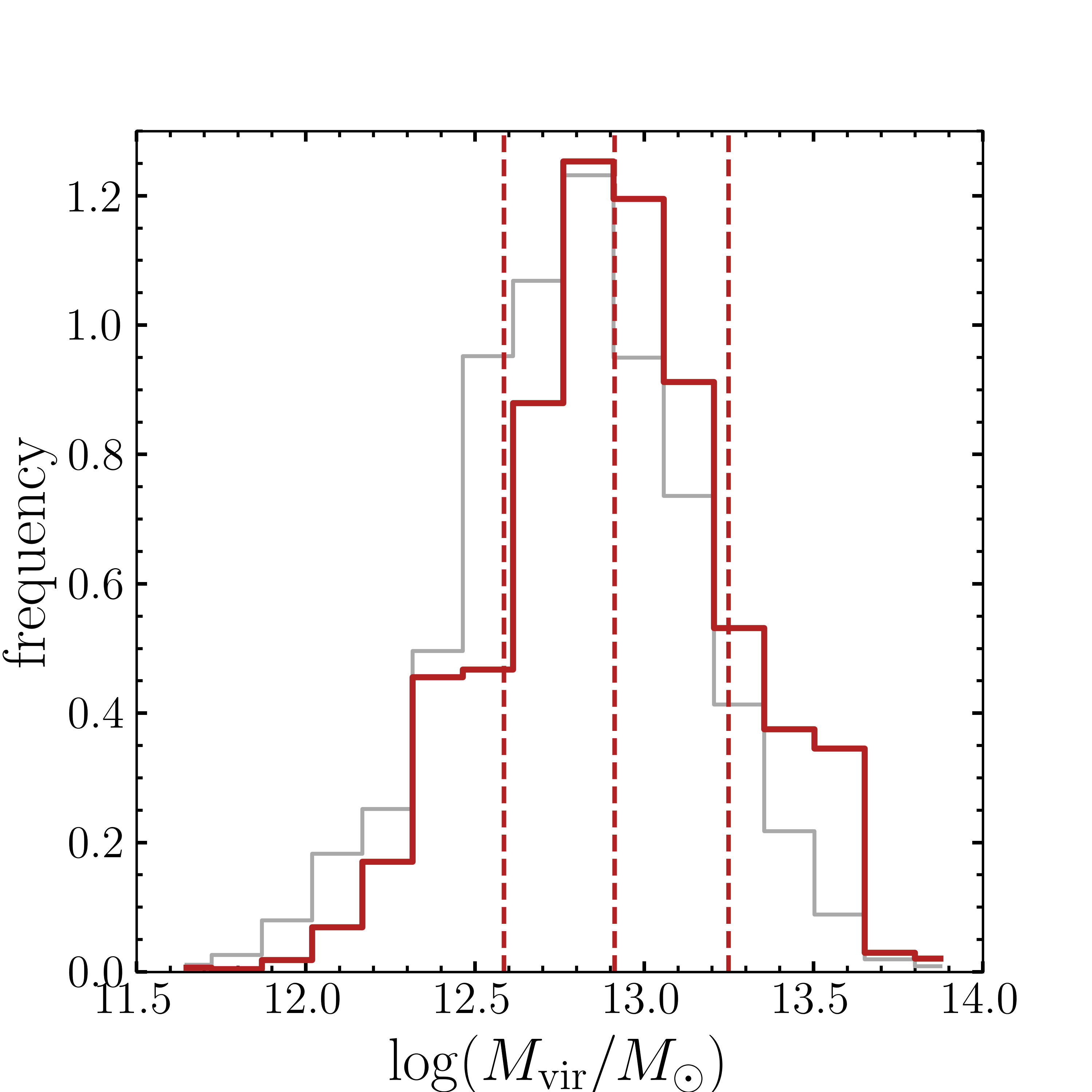
(a)

(b)

Figure S3: (a) The virial halo mass distribution in the SAM of the bright quasars ($\log(L_{\mathrm{bol}}/L_{\odot})=47.3\pm 0.3$) selected across the full-sky is shown in grey. The red curve represents the distribution of bright quasars among the selected pairs that mimic the MUDF system in the sky. (b) Same as panel (a) but for the faint quasars ($\log(L_{\mathrm{bol}}/L_{\odot})=46.3\pm 0.3$). In blue, the subsample resembling the MUDF system in the sky. All distributions are normalized to the bin width and the number of bright and faint sources obtained from their respective selections. Dashed lines indicate the mean values along with the $16^{\rm th}$ and $84^{\rm th}$ percentiles.

To obtain systems that mimic the MUDF quasars in the sky, we select all the pairs separated by a projected physical distance in the range of $400-600$ pkpc, encompassing the projected separation observed for the MUDF pair. The selection leads to a pair density of $\sim 3\times 10^{-8}$ cMpc^-3. We also include the redshift information by relying on optical rest-frame spectroscopy of the two MUDF quasars. Noting that the actual separation in velocity space for the MUDF pair is $\Delta v=600\pm 370$ km/s, we require the selected pairs to have $\Delta v\leq 1000$ km/s, resulting in a number density of $5.6\times 10^{-9}$ cMpc^-3. Thus, to find at least one pair similar to those in the MUDF, we need to sample a cube volume with a comoving side of $\sim 560$ cMpc, which is $\sim 75$ percent of the comoving cube side used in the Millenium simulation. The configuration of the MUDF is thus rare but not highly uncommon in the high-redshift Universe.

The pairs’ virial halo mass frequency distributions under this final selection are shown in Fig. S3 (red and blue curve for the bright and faint quasars). The mean values are $\log(M_{\mathrm{vir}}/M_{\odot})=12.91^{+0.34}_{-0.33}$ for QSO1 and $\log(M_{\mathrm{vir}}/M_{\odot})=12.25^{+0.46}_{-0.35}$ for QSO2. As above, the errors represent the $16^{\rm th}$ and $84^{\rm th}$ percentiles of the distributions, which we normalized to the total number of bright and faint sources obtained after the final selection. The mean masses are slightly larger than those obtained using only the bolometric luminosity selection, as imposing stringent constraints on the physical distance between halos allows us to preferentially select more biased regions than random pairs. Moreover, with this selection, we restrict halos to those that could be physically interacting. Indeed, as shown in Fig. S4 by the underlying 3D physical distance distribution along with the cumulative distribution function (red line), the $95$ percent of the systems are closer than $2.5$ pMpc and more than the $50$ precent are closer than $800$ pkpc. Thus, a large fraction of pairs in the MUDF configuration are part of the same large-scale structure and are, hence, connected or interacting in some form.

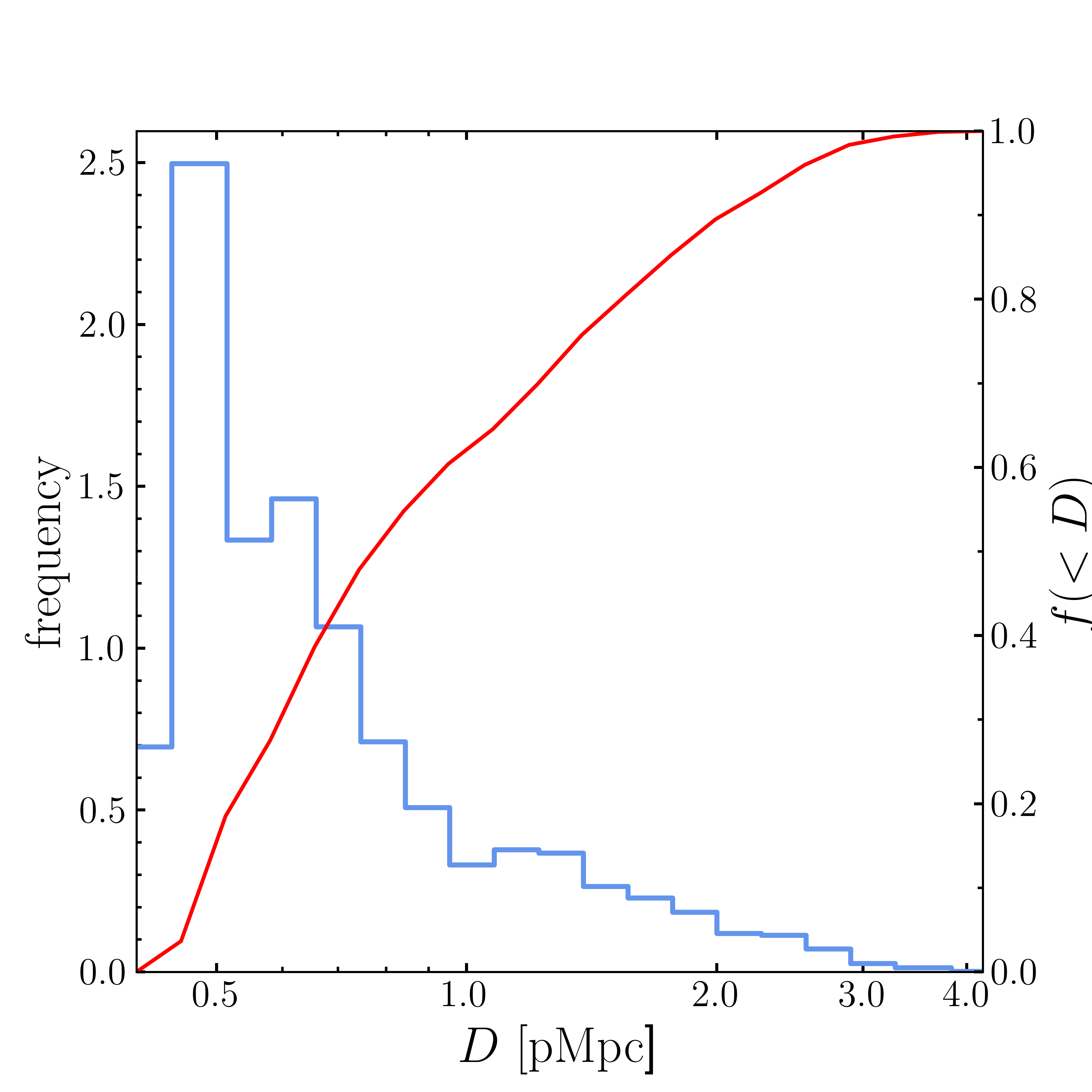
Figure S4: Frequency distribution of the 3D physical distance between each selected pair (blue histogram) and corresponding cumulative probability function (red line). The distribution is normalized to the number of selected pairs. A large fraction of MUDF pair twins are found to be connected or interacting in some form.

Analysis of hydrodynamic simulations

We used hydrodynamic cosmological simulations to explicitly verify the hypothesis that gaseous structures physically connect systems similar to the MUDF pair twins. We consider the IllustrisTNG simulations [29], focusing specifically on TNG100-1, the intermediate periodic simulation box of side length $\sim 100$ pMpc. With a gas particle mass of $1.4\times 10^{6}~{}M_{\odot}$ and a dark matter particle mass of $7.5\times 10^{6}~{}M_{\odot}$, TNG100-1 balances volume and resolution. Each TNG simulation includes a comprehensive physics model for galaxy formation and solves the coupled evolution of dark matter, cosmic gas, luminous stars, and supermassive black holes from $z=127$ to $z=0$. The simulation generates several snapshots across cosmic time, and for our analysis, we consider the one at redshift $z=3.28$, similar to the redshift of the MUDF system.

Using the halo mass distributions of the pairs similar to MUDF obtained from SAM (see Fig. S3), we select a sample of pairs within TNG100-1 with halo masses matching those of each SAM pair within $0.1$ dex. We require a projected physical distance in the range $400-600$ pkpc and a 3D distance below 5 pMpc, according to the 3D physical distance distribution of SAM in Fig. S4. We analyze separately two distinct regimes: the pairs with a 3D distance below $1$ pMpc (144 close pairs) and those at a larger distance, above $2$ pMpc (52 distant pairs).

We calculate the hydrogen density profile for each pair along the direction that connects the halos, considering all gas resolution elements within a cylinder positioned between the two halos. The cylinder’s axis corresponds to the line connecting the two halos, and the cylinder’s radius is set to $100$ pkpc to encompass potential filamentary structures in between. After normalizing the length of the cylinder by the 3D physical distance of the pair, we divide it into $17$ uniformly distributed slices to ensure a sufficient sampling of the profile. We verify that alternative slice choices do not impact the results. For each slice, we compute the hydrogen density as the total mass contained in the slice divided by the volume of the slice, assuming a primordial hydrogen fraction $X_{\mathrm{H}}=0.76$.

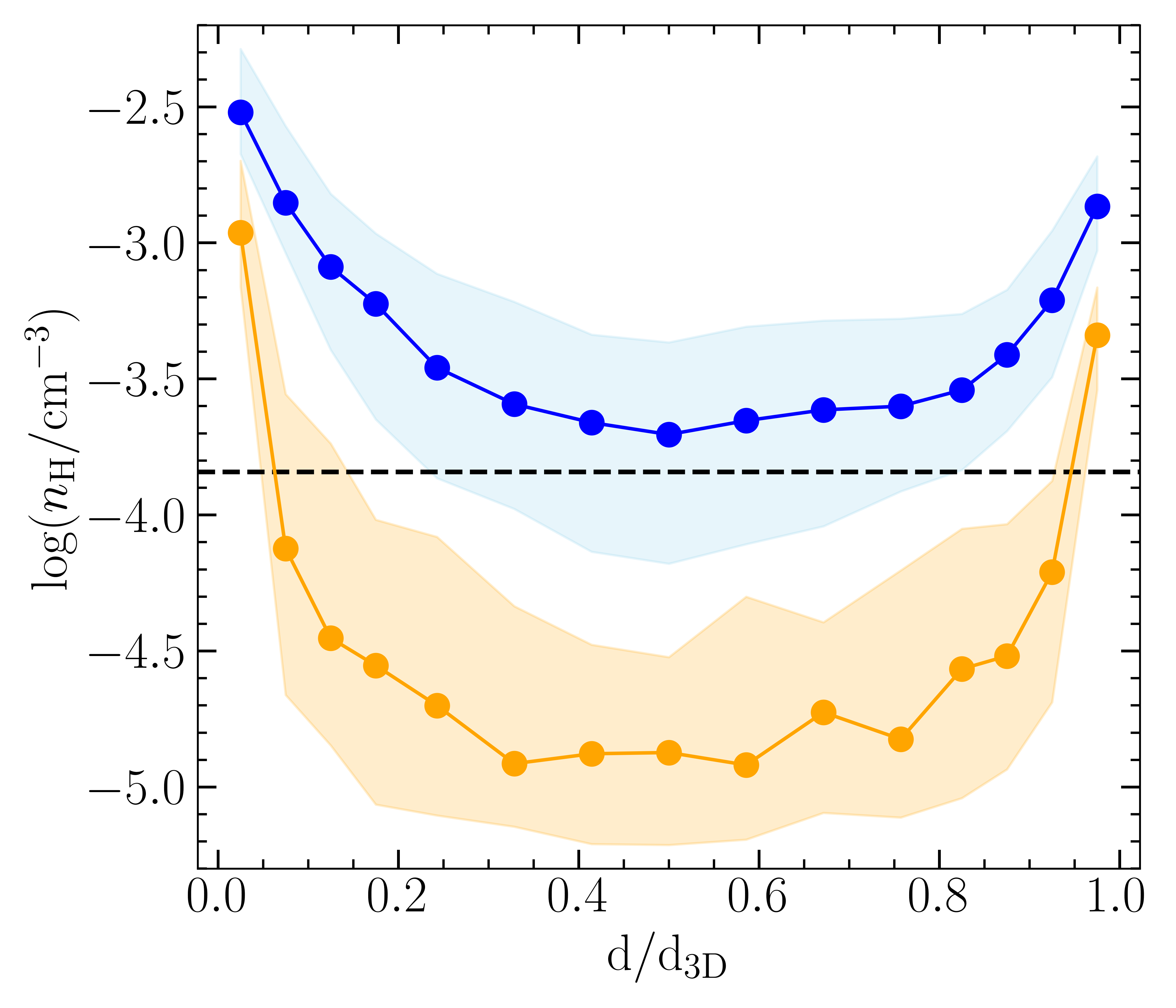
Figure S5: The median hydrogen density profile along the filament of the selected close and distant pairs separated by a 3D distance of $<1$ pMpc (blue line) and $>2$ pMpc (orange line). Both profiles are shown as a function of the normalized 3D physical distance between the two halos. The shaded regions represent the $16^{\rm th}$ and $84^{\rm th}$ percentiles of the profiles distribution. The black dashed lines represent ten times the hydrogen critical density of the Universe at this redshift, the threshold used to compare the properties of the two subsamples.

The median density profiles of the pairs, both those with a 3D distance below 1 pMpc and those above 2 pMpc, are shown in Fig. S5. The sky-blue and orange-shaded regions mark the $16^{\rm th}$ and $84^{\rm th}$ percentiles of the profile distribution. Pairs with a 3D distance below 1 pMpc are typically connected by a denser medium (see, e.g., the left panel of Fig. 4), exhibiting a smooth transition from the CGM to the IGM, with a minimum median hydrogen density value of $\sim 10^{-3.7}$ cm^-3. In contrast, distant pairs with a 3D distance above 2 pMpc are not typically connected by an identifiable overdense structure and display a steeper radial hydrogen density profile, reaching a minimum median hydrogen density of $\sim 10^{-4.8}$ cm^-3. We interpret this result as statistical evidence of more overdense filaments connecting the close pairs. To further quantify the occurrence of connecting filaments between the two subsamples, we also calculate the hydrogen density within a cylinder of radius $100$ pkpc in the region ranging from $0.25d_{\mathrm{3D}}$ to $0.75d_{\mathrm{3D}}$, focusing solely on the contribution of the filamentary structure and excluding the region associated to the CGM. We determine the fraction of pairs with a filament density value above a threshold of ten times the critical hydrogen density at redshift $\sim 3.22$, which is $\sim 1.4\times 10^{-5}$ cm^-3. This reference value aligns to the strongest absorbers observed in tracing the Ly$\alpha$ forest in quasar spectra (e.g., [6]). Most of the systems with a 3D distance below 1 pMpc ($75$ percent) exhibit densities exceeding this threshold, while only $8$ percent of the systems with a 3D distance above 2 pMpc exceed this threshold. We thus conclude that the former subsample contains systems truly connected by a dense gaseous filament.

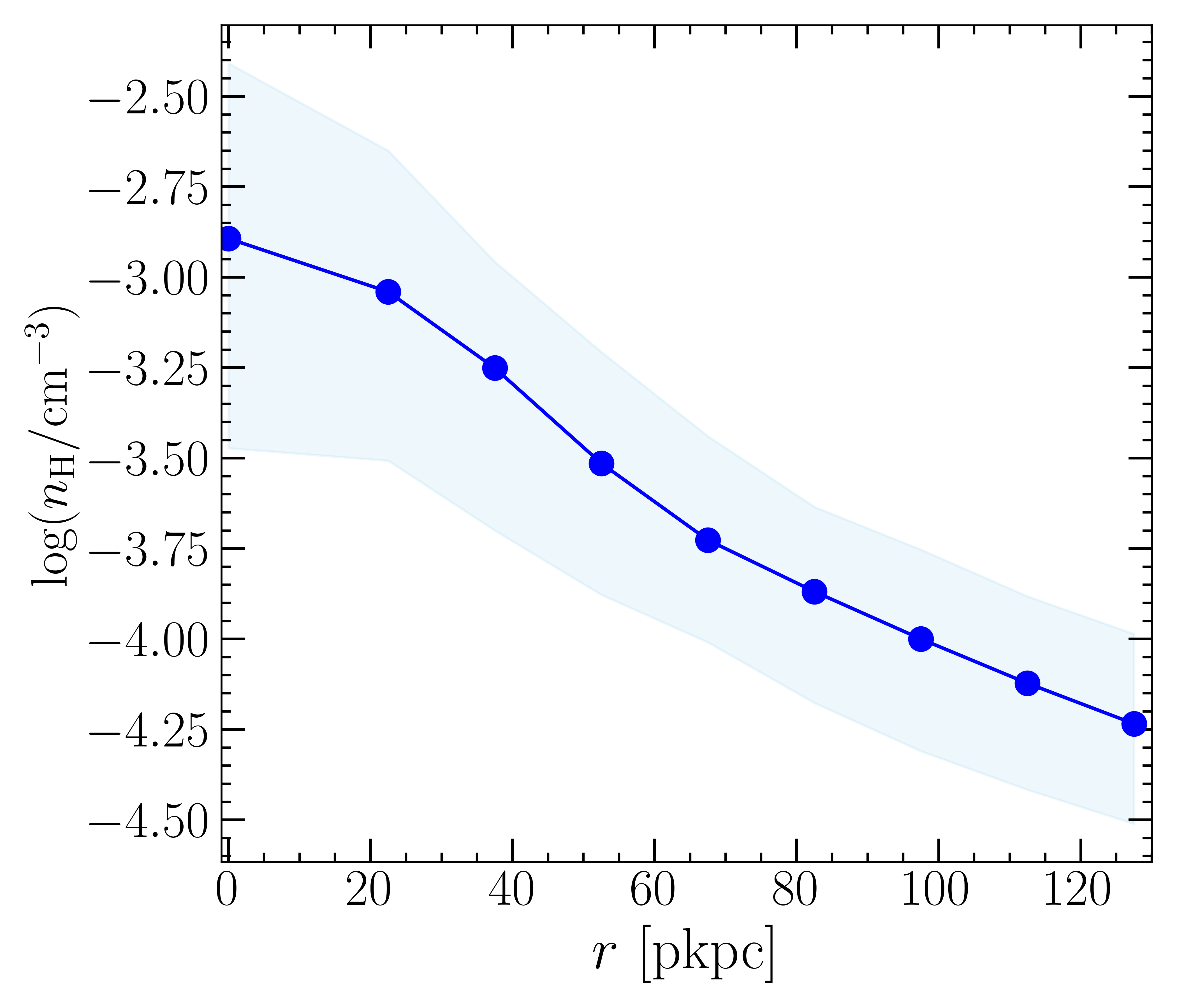
Figure S6: The transverse median hydrogen density profile of the physically connected pairs separated by a 3D distance $<1$ pMpc. The sky-blue colored region represents the $16^{\rm th}$ and $84^{\rm th}$ percentiles of the profiles distribution.

We also compute the filament’s transverse hydrogen profile for the physically connected pairs with a 3D distance below 1 pMpc. After selecting the filamentary structure as described above, we define the direction of the filament’s spine, computing the two highest density points below and above $0.5d_{\mathrm{3D}}$. With this approach, we can account for filaments not perfectly aligned with the axis joining the two halos, as done in our analysis of the transverse surface brightness profile in the MUSE data. Knowing the filament’s orientation, we consider a cylinder along the spine direction with a radius of $130$ pkpc, which we divide into different shells with a width of $\Delta r=15$ pkpc. As above, we estimate the hydrogen density as the total gas mass contained in a given shell divided by the volume of the shell, after accounting for the hydrogen fraction $X_{\mathrm{H}}$. The obtained profile is shown in Fig. S6. From the obtained profile, we can infer that the physically connected pairs have a filamentary structure with a median hydrogen density of $\approx 10^{-2.8}$ cm^-3 in the densest part along the filament’s spine and that the density falls from the center of the filament with an exponential decline radius of $40\pm 15$ pkpc.

To more closely compare the MUSE observations with the results of simulations, we derive the surface brightness maps assuming that the diffuse gas emission originates from recombinations and collisional excitation. For each gas resolution element, we calculate the emissivities from the equations

$$\epsilon_{\mathrm{Ly\alpha}}^{\mathrm{rec}}=\frac{h\nu_{\mathrm{Ly\alpha}}}{4\pi}\alpha_{\mathrm{eff}}(T)(1-\eta)^{2}n_{\mathrm{H}}^{2},$$ (2)

and

$$\epsilon_{\mathrm{Ly\alpha}}^{\mathrm{coll}}=\frac{h\nu_{\mathrm{Ly\alpha}}}{4\pi}\gamma_{\mathrm{1s2p}}(T)\eta(1-\eta)n_{\mathrm{H}}^{2}.$$ (3)

The emissivities depend on the squared number density of neutral hydrogen, $n_{\mathrm{H}}$. Recombinations are calculated assuming a case A scenario with the temperature-dependent recombination coefficient $\alpha_{\mathrm{eff}}(T)$ from Hui & Gnedin [38] and the collisional excitation coefficient $\gamma_{\mathrm{1s2p}}(T)$ from Scholz & Walters [39]. Assuming ionization equilibrium, the neutral hydrogen fraction, $\eta=n_{\mathrm{HI}}/n_{\mathrm{H}}$, is calculated following Appendix A2 in Rahmati et al. [40], as done within the simulation. The temperature of each cell gas is computed assuming a perfect monoatomic gas from the internal energy $u$ given by the simulation, using the relation $T_{\mathrm{cell}}=(\gamma-1)\mu m_{\mathrm{p}}u/k_{\mathrm{B}}$, where $\gamma=5/3$ and $\mu=4/(1+3X_{\mathrm{H}}+4X_{\mathrm{H}}x_{\mathrm{e}})$ is the mean molecular weight calculated with the electron abundance $x_{\mathrm{e}}$ given by the simulation. We include only gas with densities $n_{H}<0.1~{}\rm cm^{-3}$, i.e., outside the imposed equation of state. Due to the presence of the quasars in our observations, we also consider a maximal fluorescence model, assuming that the ionizing sources are bright enough to ionize the surrounding medium fully. We, therefore, calculate the emissivity of the gas due to Ly$\alpha$ recombination radiation following a simplified relation where $\eta$ is assumed to be zero in the equation (2) (see e.g. de Beer et al. [24]). Finally, using the public package Py-SPHViewer [41], we integrate along the line of sight (assumed as $z$) the total emissivity to obtain the surface brightness images of the selected pairs (see, e.g., the center panel of Fig. 4).

Figure S7: From the top to the bottom, the panels display the median transverse surface brightness profiles of the selected pairs with a 3D distance below 1 pMpc in TNG300-1, TNG100-1 and TNG50-1, respectively. The blue line represents the emission contribution from recombinations only, while the orange line represents both recombinations and collisional excitations. The red points represent the measured data and their errors for the transverse surface brightness profile in MUDF. The shaded regions denote the $16^{\rm th}$ and $84^{\rm th}$ percentiles of the profile distributions. In the central panel, the emission contribution from the maximal fluorescence model is also shown as a black line.

Using the same approach followed in our observations (see also the right panel of Fig. S2), we measure the transverse surface brightness profile using 9 rectangular boxes for each pair up to a distance of $100$ pkpc on either side relative to the direction connecting the two halos. Once again, the boxes can be positioned off-axis to that direction, ensuring the emission peak is at $R=0$. To exclude the contribution from the CGM of the two main halos (but leaving possible contribution from other embedded halos), each box’s length encompasses only the projected filament region, defined by maintaining a distance of $0.25d_{\mathrm{2D}}$ from each halo, which is similar to the transition radius measured in the MUDF. As both emission processes considered here depend on the density square, we explicitly test the robustness of these predictions as a function of resolution, comparing results across the three boxes available in the IllustrisTNG simulation (TNG300-1, TNG100-1, and TNG50-1), covering a range of $\approx 200$ in volume and $\approx 130$ in mass. Applying the pair selection described above for TNG100-1 yields 710 pairs below 1 pMpc in TNG300-1 and 24 in TNG50-1.

Fig. S7 compares the median emission profile from both recombinations and collisional excitations (orange line), as well as considering only recombinations (blue line), along with the $16^{\rm th}$ and $84^{\rm th}$ percentiles. We observe that, on average, the result is not strongly sensitive at the different resolutions of TNG, implying that the typical densities within the mildly overdense filaments are reasonably converged at these scales, a result also found in simulations of the Ly$\alpha$ forest. We also observe that the maximal fluorescence model produces a median surface brightness profile that agrees remarkably well, within a mean factor of $\approx 2$, with the recombination model. Thus, the simulations predict that the mostly optically thin filaments have temperature-dependent coefficients and ionization fractions close to the maximal fluorescence conditions. This analysis concludes that the derived surface brightness maps are generally robust relative to the assumptions made.

When comparing the predicted profiles with the observational data points measured in the MUDF up to $\approx 70$ pkpc, where the measurements exceed the detection limit of the NB image, we observe that the maximal fluorescence and the recombination models lie below the observed surface brightness. This indicates that the densities predicted by the simulations cannot be too high compared to real values as, otherwise, the simulated profiles would exceed the observed ones. Moreover, observations and simulations can be brought into agreement by boosting recombination radiation by a factor of $\approx 9$ in the surface brightness, i.e., requiring an increase in density by a factor of no more than $\approx 3$. Hence, the simulated densities cannot be much lower than the true values. Such a boost should also be considered a maximum correction that must be applied due to the presence of additional photons from collisions. Indeed, when including collisional excitations, despite the more uncertain nature of this calculation due to the high sensitivity to temperature, the profile shifts upward, especially in the inner $\approx 25~{}$pkpc. We also note that the $0.1~{}\rm cm^{-3}$ cut is quite stringent, as we explicitly tested that the denser and more neutral gas around $\approx 0.1-0.3~{}\rm cm^{-3}$ is a significant source of photons. Including that phase, we observe a good agreement between the surface brightness level predicted by the simulations and the MUDF filament, with both profiles lying at $\approx 10^{-19}~{}\rm erg~{}s^{-1}~{}cm^{-2}~{}arcsec^{-2}$ in the range $R\approx 20-40$ pkpc. Our analysis also neglects scattering processes, predicted to be significant in the cosmic web [30], that redistribute photons from regions of high to low surface brightness. Hence, discrepancies are not particularly concerning. Overall, this analysis implies a satisfactory agreement between the density predicted in the cold dark matter model and what is in our Universe.

Furthermore, there is no special reason why the MUDF filament should agree with the distribution median. Considering this aspect, we searched among the simulated surface brightness profiles for a pair that resembles the MUDF system more closely. One such MUDF twin is shown in Fig. 4, where we see a transverse profile that matches the observations. Hence, filaments with observed characteristics comparable to the MUDF exist in the cold dark matter paradigm, and our study paves the way for further quantitative analysis of the properties of the cosmic web within our cosmological model.

References

- \bibcommenthead
- Frenk et al. [1988] Frenk, C.S., White, S.D.M., Davis, M., Efstathiou, G.: The Formation of Dark Halos in a Universe Dominated by Cold Dark Matter. ApJ 327, 507 (1988) https://doi.org/10.1086/166213
- Cen et al. [1994] Cen, R., Miralda-Escudé, J., Ostriker, J.P., Rauch, M.: Gravitational Collapse of Small-Scale Structure as the Origin of the Lyman-Alpha Forest. ApJ 437, 9 (1994) https://doi.org/10.1086/187670 arXiv:astro-ph/9409017 [astro-ph]
- Lukić et al. [2015] Lukić, Z., Stark, C.W., Nugent, P., White, M., Meiksin, A.A., Almgren, A.: The Lyman forest in optically thin hydrodynamical simulations. MNRAS 446(4), 3697–3724 (2015) https://doi.org/10.1093/mnras/stu2377 arXiv:1406.6361 [astro-ph.CO]
- Peacock et al. [2001] Peacock, J.A., Cole, S., Norberg, P., Baugh, C.M., Bland-Hawthorn, J., Bridges, T., Cannon, R.D., Colless, M., Collins, C., Couch, W., Dalton, G., Deeley, K., De Propris, R., Driver, S.P., Efstathiou, G., Ellis, R.S., Frenk, C.S., Glazebrook, K., Jackson, C., Lahav, O., Lewis, I., Lumsden, S., Maddox, S., Percival, W.J., Peterson, B.A., Price, I., Sutherland, W., Taylor, K.: A measurement of the cosmological mass density from clustering in the 2dF Galaxy Redshift Survey. Nature 410(6825), 169–173 (2001) https://doi.org/10.1038/35065528 arXiv:astro-ph/0103143 [astro-ph]
- Tempel et al. [2014] Tempel, E., Stoica, R.S., Martínez, V.J., Liivamägi, L.J., Castellan, G., Saar, E.: Detecting filamentary pattern in the cosmic web: a catalogue of filaments for the SDSS. MNRAS 438(4), 3465–3482 (2014) https://doi.org/10.1093/mnras/stt2454 arXiv:1308.2533 [astro-ph.CO]
- Rauch [1998] Rauch, M.: The Lyman Alpha Forest in the Spectra of QSOs. ARA&A 36, 267–316 (1998) https://doi.org/10.1146/annurev.astro.36.1.267 arXiv:astro-ph/9806286 [astro-ph]
- Bacon et al. [2010] Bacon, R., Accardo, M., Adjali, L., Anwand, H., Bauer, S., Biswas, I., Blaizot, J., Boudon, D., Brau-Nogue, S., Brinchmann, J., Caillier, P., Capoani, L., Carollo, C.M., Contini, T., Couderc, P., Daguisé, E., Deiries, S., Delabre, B., Dreizler, S., Dubois, J., Dupieux, M., Dupuy, C., Emsellem, E., Fechner, T., Fleischmann, A., François, M., Gallou, G., Gharsa, T., Glindemann, A., Gojak, D., Guiderdoni, B., Hansali, G., Hahn, T., Jarno, A., Kelz, A., Koehler, C., Kosmalski, J., Laurent, F., Le Floch, M., Lilly, S.J., Lizon, J.-L., Loupias, M., Manescau, A., Monstein, C., Nicklas, H., Olaya, J.-C., Pares, L., Pasquini, L., Pécontal-Rousset, A., Pelló, R., Petit, C., Popow, E., Reiss, R., Remillieux, A., Renault, E., Roth, M., Rupprecht, G., Serre, D., Schaye, J., Soucail, G., Steinmetz, M., Streicher, O., Stuik, R., Valentin, H., Vernet, J., Weilbacher, P., Wisotzki, L., Yerle, N.: The MUSE second-generation VLT instrument. In: McLean, I.S., Ramsay, S.K., Takami, H. (eds.) Ground-based and Airborne Instrumentation for Astronomy III. Society of Photo-Optical Instrumentation Engineers (SPIE) Conference Series, vol. 7735, p. 773508 (2010). https://doi.org/10.1117/12.856027
- Umehata et al. [2019] Umehata, H., Fumagalli, M., Smail, I., Matsuda, Y., Swinbank, A.M., Cantalupo, S., Sykes, C., Ivison, R.J., Steidel, C.C., Shapley, A.E., Vernet, J., Yamada, T., Tamura, Y., Kubo, M., Nakanishi, K., Kajisawa, M., Hatsukade, B., Kohno, K.: Gas filaments of the cosmic web located around active galaxies in a protocluster. Science 366(6461), 97–100 (2019) https://doi.org/10.1126/science.aaw5949 arXiv:1910.01324 [astro-ph.GA]
- Bacon et al. [2021] Bacon, R., Mary, D., Garel, T., Blaizot, J., Maseda, M., Schaye, J., Wisotzki, L., Conseil, S., Brinchmann, J., Leclercq, F., Abril-Melgarejo, V., Boogaard, L., Bouché, N.F., Contini, T., Feltre, A., Guiderdoni, B., Herenz, C., Kollatschny, W., Kusakabe, H., Matthee, J., Michel-Dansac, L., Nanayakkara, T., Richard, J., Roth, M., Schmidt, K.B., Steinmetz, M., Tresse, L., Urrutia, T., Verhamme, A., Weilbacher, P.M., Zabl, J., Zoutendijk, S.L.: The MUSE Extremely Deep Field: The cosmic web in emission at high redshift. A&A 647, 107 (2021) https://doi.org/10.1051/0004-6361/202039887 arXiv:2102.05516 [astro-ph.CO]
- Cai et al. [2018] Cai, Z., Hamden, E., Matuszewski, M., Prochaska, J.X., Li, Q., Cantalupo, S., Arrigoni Battaia, F., Martin, C., Neill, J.D., O’Sullivan, D., Wang, R., Moore, A., Morrissey, P.: Keck/Palomar Cosmic Web Imagers Reveal an Enormous Ly Nebula in an Extremely Overdense Quasi-stellar Object Pair Field at z = 2.45. ApJ 861(1), 3 (2018) https://doi.org/10.3847/2041-8213/aacce6 arXiv:1803.10781 [astro-ph.GA]
- Arrigoni Battaia et al. [2019] Arrigoni Battaia, F., Obreja, A., Prochaska, J.X., Hennawi, J.F., Rahmani, H., Bañados, E., Farina, E.P., Cai, Z., Man, A.: Discovery of intergalactic bridges connecting two faint z 3 quasars. A&A 631, 18 (2019) https://doi.org/10.1051/0004-6361/201936211 arXiv:1909.00829 [astro-ph.GA]
- Martin et al. [2023] Martin, D.C., Darvish, B., Lin, Z., Cen, R., Matuszewski, M., Morrissey, P., Neill, J.D., Moore, A.M.: Extensive diffuse Lyman- emission correlated with cosmic structure. Nature Astronomy 7, 1390–1401 (2023) https://doi.org/10.1038/s41550-023-02054-1
- Revalski et al. [2023] Revalski, M., Rafelski, M., Fumagalli, M., Fossati, M., Pirzkal, N., Sunnquist, B., Prichard, L.J., Henry, A., Bagley, M., Dutta, R., Papini, G., Battaia, F.A., D’Odorico, V., Dayal, P., Estrada-Carpenter, V., Lofthouse, E.K., Lusso, E., Morris, S.L., Nedkova, K.V., Papovich, C., Peroux, C.: The MUSE Ultra Deep Field (MUDF). III. Hubble Space Telescope WFC3 Grism Spectroscopy and Imaging. ApJS 265(2), 40 (2023) https://doi.org/10.3847/1538-4365/acb8ae arXiv:2302.01345 [astro-ph.GA]
- Fossati et al. [2019] Fossati, M., Fumagalli, M., Lofthouse, E.K., D’Odorico, V., Lusso, E., Cantalupo, S., Cooke, R.J., Cristiani, S., Haardt, F., Morris, S.L., Peroux, C., Prichard, L.J., Rafelski, M., Smail, I., Theuns, T.: The MUSE Ultra Deep Field (MUDF). II. Survey design and the gaseous properties of galaxy groups at . Monthly Notices of the Royal Astronomical Society 490(1), 1451–1469 (2019) https://doi.org/10.1093/mnras/stz2693 https://academic.oup.com/mnras/article-pdf/490/1/1451/30152206/stz2693.pdf
- Lusso et al. [2019] Lusso, E., Fumagalli, M., Fossati, M., Mackenzie, R., Bielby, R.M., Arrigoni Battaia, F., Cantalupo, S., Cooke, R., Cristiani, S., Dayal, P., D’Odorico, V., Haardt, F., Lofthouse, E., Morris, S., Peroux, C., Prichard, L., Rafelski, M., Simcoe, R., Swinbank, A.M., Theuns, T.: The MUSE Ultra Deep Field (MUDF) - I. Discovery of a group of Ly nebulae associated with a bright z 3.23 quasar pair. MNRAS 485(1), 62–67 (2019) https://doi.org/%****␣sn-article.bbl␣Line␣500␣****10.1093/mnrasl/slz032 arXiv:1903.00483 [astro-ph.GA]
- Vogelsberger et al. [2014] Vogelsberger, M., Genel, S., Springel, V., Torrey, P., Sijacki, D., Xu, D., Snyder, G., Nelson, D., Hernquist, L.: Introducing the Illustris Project: simulating the coevolution of dark and visible matter in the Universe. MNRAS 444(2), 1518–1547 (2014) https://doi.org/10.1093/mnras/stu1536 arXiv:1405.2921 [astro-ph.CO]
- Rahmati et al. [2015] Rahmati, A., Schaye, J., Bower, R.G., Crain, R.A., Furlong, M., Schaller, M., Theuns, T.: The distribution of neutral hydrogen around high-redshift galaxies and quasars in the EAGLE simulation. MNRAS 452(2), 2034–2056 (2015) https://doi.org/10.1093/mnras/stv1414 arXiv:1503.05553 [astro-ph.CO]
- Cantalupo et al. [2005] Cantalupo, S., Porciani, C., Lilly, S.J., Miniati, F.: Fluorescent Ly Emission from the High-Redshift Intergalactic Medium. ApJ 628(1), 61–75 (2005) https://doi.org/10.1086/430758 arXiv:astro-ph/0504015 [astro-ph]
- Borisova et al. [2016] Borisova, E., Cantalupo, S., Lilly, S.J., Marino, R.A., Gallego, S.G., Bacon, R., Blaizot, J., Bouché, N., Brinchmann, J., Carollo, C.M., Caruana, J., Finley, H., Herenz, E.C., Richard, J., Schaye, J., Straka, L.A., Turner, M.L., Urrutia, T., Verhamme, A., Wisotzki, L.: Ubiquitous Giant Ly Nebulae around the Brightest Quasars at z 3.5 Revealed with MUSE. ApJ 831(1), 39 (2016) https://doi.org/10.3847/0004-637X/831/1/39 arXiv:1605.01422 [astro-ph.GA]
- Arrigoni Battaia et al. [2019] Arrigoni Battaia, F., Hennawi, J.F., Prochaska, J.X., Oñorbe, J., Farina, E.P., Cantalupo, S., Lusso, E.: QSO MUSEUM I: a sample of 61 extended Ly -emission nebulae surrounding quasars. MNRAS 482(3), 3162–3205 (2019) https://doi.org/10.1093/mnras/sty2827 arXiv:1808.10857 [astro-ph.GA]
- Mackenzie et al. [2021] Mackenzie, R., Pezzulli, G., Cantalupo, S., Marino, R.A., Lilly, S., Muzahid, S., Matthee, J., Schaye, J., Wisotzki, L.: Revealing the impact of quasar luminosity on giant Ly nebulae. MNRAS 502(1), 494–509 (2021) https://doi.org/10.1093/mnras/staa3277 arXiv:2010.12589 [astro-ph.GA]
- Nielsen et al. [2023] Nielsen, N.M., Fisher, D.B., Kacprzak, G.G., Chisholm, J., Martin, D.C., Reichardt Chu, B., Sandstrom, K.M., Rickards Vaught, R.J.: Revealing the disk-circumgalactic medium transition with emission mapping. arXiv e-prints, 2311–00856 (2023) https://doi.org/10.48550/arXiv.2311.00856 arXiv:2311.00856 [astro-ph.GA]
- Fossati et al. [2021] Fossati, M., Fumagalli, M., Lofthouse, E.K., Dutta, R., Cantalupo, S., Arrigoni Battaia, F., Fynbo, J.P.U., Lusso, E., Murphy, M.T., Prochaska, J.X., Theuns, T., Cooke, R.J.: MUSE analysis of gas around galaxies (MAGG) - III. The gas and galaxy environment of z = 3-4.5 quasars. MNRAS 503(2), 3044–3064 (2021) https://doi.org/10.1093/mnras/stab660 arXiv:2103.01960 [astro-ph.GA]
- de Beer et al. [2023] de Beer, S., Cantalupo, S., Travascio, A., Pezzulli, G., Galbiati, M., Fossati, M., Fumagalli, M., Lazeyras, T., Pensabene, A., Theuns, T., Wang, W.: Resolving the physics of quasar Ly nebulae (RePhyNe): I. Constraining quasar host halo masses through circumgalactic medium kinematics. MNRAS 526(2), 1850–1873 (2023) https://doi.org/10.1093/mnras/stad2682 arXiv:2309.01506 [astro-ph.GA]
- Wilde et al. [2023] Wilde, M.C., Tchernyshyov, K., Werk, J.K., Tripp, T.M., Burchett, J.N., Prochaska, J.X., Tejos, N., Lehner, N., Bordoloi, R., O’Meara, J.M., Tumlinson, J., Howk, J.C.: CGM2 + CASBaH: The Mass Dependence of H I Ly-Galaxy Clustering and the Extent of the CGM. ApJ 948(2), 114 (2023) https://doi.org/10.3847/1538-4357/acc85b arXiv:2301.02718 [astro-ph.GA]
- Izquierdo-Villalba et al. [2019] Izquierdo-Villalba, D., Bonoli, S., Spinoso, D., Rosas-Guevara, Y., Henriques, B.M.B., Hernández-Monteagudo, C.: The build-up of pseudo-bulges in a hierarchical universe. MNRAS 488(1), 609–632 (2019) https://doi.org/10.1093/mnras/stz1694 arXiv:1901.10490 [astro-ph.GA]
- Izquierdo-Villalba et al. [2020] Izquierdo-Villalba, D., Bonoli, S., Dotti, M., Sesana, A., Rosas-Guevara, Y., Spinoso, D.: From galactic nuclei to the halo outskirts: tracing supermassive black holes across cosmic history and environments. MNRAS 495(4), 4681–4706 (2020) https://doi.org/10.1093/mnras/staa1399 arXiv:2001.10548 [astro-ph.GA]
- Lusso et al. [2023] Lusso, E., Nardini, E., Fumagalli, M., Fossati, M., Arrigoni Battaia, F., Revalski, M., Rafelski, M., D’Odorico, V., Peroux, C., Cristiani, S., Dayal, P., Haardt, F., Lofthouse, E.K.: The MUSE Ultra Deep Field (MUDF). IV. A pair of X-ray weak quasars at the heart of two extended Ly nebulae. MNRAS 525(3), 4388–4404 (2023) https://doi.org/10.1093/mnras/stad2564 arXiv:2308.12993 [astro-ph.GA]
- Nelson et al. [2019] Nelson, D., Springel, V., Pillepich, A., Rodriguez-Gomez, V., Torrey, P., Genel, S., Vogelsberger, M., Pakmor, R., Marinacci, F., Weinberger, R., Kelley, L., Lovell, M., Diemer, B., Hernquist, L.: The IllustrisTNG simulations: public data release. Computational Astrophysics and Cosmology 6(1), 2 (2019) https://doi.org/10.1186/s40668-019-0028-x arXiv:1812.05609 [astro-ph.GA]
- Byrohl and Nelson [2023] Byrohl, C., Nelson, D.: The cosmic web in Lyman-alpha emission. MNRAS 523(4), 5248–5273 (2023) https://doi.org/10.1093/mnras/stad1779 arXiv:2212.08666 [astro-ph.GA]
- Weilbacher et al. [2014] Weilbacher, P.M., Streicher, O., Urrutia, T., Pécontal-Rousset, A., Jarno, A., Bacon, R.: The MUSE Data Reduction Pipeline: Status after Preliminary Acceptance Europe. In: Manset, N., Forshay, P. (eds.) Astronomical Data Analysis Software and Systems XXIII. Astronomical Society of the Pacific Conference Series, vol. 485, p. 451 (2014). https://doi.org/10.48550/arXiv.1507.00034
- Cantalupo et al. [2019] Cantalupo, S., Pezzulli, G., Lilly, S.J., Marino, R.A., Gallego, S.G., Schaye, J., Bacon, R., Feltre, A., Kollatschny, W., Nanayakkara, T., Richard, J., Wendt, M., Wisotzki, L., Prochaska, J.X.: The large- and small-scale properties of the intergalactic gas in the Slug Ly nebula revealed by MUSE He II emission observations. MNRAS 483(4), 5188–5204 (2019) https://doi.org/10.1093/mnras/sty3481 arXiv:1811.11783 [astro-ph.GA]
- Lofthouse et al. [2019] Lofthouse, E.K., Fumagalli, M., Fossati, M., O’Meara, J.M., Murphy, M.T., Christensen, L., Prochaska, J.X., Cantalupo, S., Bielby, R.M., Cooke, R.J., Lusso, E., Morris, S.L.: MUSE Analysis of Gas around Galaxies (MAGG) – I: Survey design and the environment of a near pristine gas cloud at z 3.5. Monthly Notices of the Royal Astronomical Society 491(2), 2057–2074 (2019) https://doi.org/10.1093/mnras/stz3066 https://academic.oup.com/mnras/article-pdf/491/2/2057/36236111/stz3066.pdf
- Arrigoni Battaia et al. [2023] Arrigoni Battaia, F., Obreja, A., Costa, T., Farina, E.P., Cai, Z.: The Luminosity-Area Relation of Quasars’ Ly Nebulae. ApJ 952(1), 24 (2023) https://doi.org/10.3847/2041-8213/ace42b arXiv:2306.14334 [astro-ph.GA]
- Lu et al. [2024] Lu, Y.S., Mandelker, N., Oh, S.P., Dekel, A., van den Bosch, F.C., Springel, V., Nagai, D., van de Voort, F.: The structure and dynamics of massive high-z cosmic-web filaments: three radial zones in filament cross-sections. MNRAS 527(4), 11256–11287 (2024) https://doi.org/10.1093/mnras/stad3779 arXiv:2306.03966 [astro-ph.CO]
- Henriques et al. [2015] Henriques, B.M.B., White, S.D.M., Thomas, P.A., Angulo, R., Guo, Q., Lemson, G., Springel, V., Overzier, R.: Galaxy formation in the Planck cosmology - I. Matching the observed evolution of star formation rates, colours and stellar masses. MNRAS 451(3), 2663–2680 (2015) https://doi.org/10.1093/mnras/stv705 arXiv:1410.0365 [astro-ph.GA]
- Springel et al. [2005] Springel, V., White, S.D.M., Jenkins, A., Frenk, C.S., Yoshida, N., Gao, L., Navarro, J., Thacker, R., Croton, D., Helly, J., Peacock, J.A., Cole, S., Thomas, P., Couchman, H., Evrard, A., Colberg, J., Pearce, F.: Simulations of the formation, evolution and clustering of galaxies and quasars. Nature 435(7042), 629–636 (2005) https://doi.org/10.1038/nature03597 arXiv:astro-ph/0504097 [astro-ph]
- Hui and Gnedin [1997] Hui, L., Gnedin, N.Y.: Equation of state of the photoionized intergalactic medium. Monthly Notices of the Royal Astronomical Society 292(1), 27–42 (1997) https://doi.org/10.1093/mnras/292.1.27 https://academic.oup.com/mnras/article-pdf/292/1/27/4004449/292-1-27.pdf
- Scholz and Walters [1991] Scholz, T.T., Walters, H.R.J.: Collisional Rates and Cooling within Atomic Hydrogen Plasmas. ApJ 380, 302 (1991) https://doi.org/10.1086/170587
- Rahmati et al. [2013] Rahmati, A., Pawlik, A.H., Raičević, M., Schaye, J.: On the evolution of the H I column density distribution in cosmological simulations. MNRAS 430(3), 2427–2445 (2013) https://doi.org/10.1093/mnras/stt066 arXiv:1210.7808 [astro-ph.CO]
- Benitez-Llambay [2015] Benitez-Llambay, A.: py-sphviewer: Py-SPHViewer v1.0.0 (2015). https://doi.org/10.5281/zenodo.21703 . http://dx.doi.org/10.5281/zenodo.21703