Cubic regularized subspace Newton for non-convex optimization

Abstract

This paper addresses the optimization problem of minimizing non-convex continuous functions, which is relevant in the context of high-dimensional machine learning applications characterized by over-parametrization. We analyze a randomized coordinate second-order method named SSCN which can be interpreted as applying cubic regularization in random subspaces. This approach effectively reduces the computational complexity associated with utilizing second-order information, rendering it applicable in higher-dimensional scenarios. Theoretically, we establish convergence guarantees for non-convex functions, with interpolating rates for arbitrary subspace sizes and allowing inexact curvature estimation. When increasing subspace size, our complexity matches $\mathcal{O}(\epsilon^{-3/2})$ of the cubic regularization (CR) rate. Additionally, we propose an adaptive sampling scheme ensuring exact convergence rate of $\mathcal{O}(\epsilon^{-3/2},\epsilon^{-3})$ to a second-order stationary point, even without sampling all coordinates. Experimental results demonstrate substantial speed-ups achieved by SSCN compared to conventional first-order methods.

1 Introduction

In this paper, we address the problem of minimizing an objective function of the form $\min_{{\bf x}\in{\mathbb{R}}^{n}}f({\bf x})$, where $f:{\mathbb{R}}^{n}\to{\mathbb{R}}$ is a two-times differentiable, possibly non-convex function, having Lipschitz continuous gradient and Hessian. Our focus lies on scenarios where the dimension $n$ has the potential to be significantly large, a context that holds relevance for numerous machine learning applications. This pertains particularly to situations in which models tend to exhibit a large number of parameters, commonly referred to as over-parametrization. One method of choice to optimize the objective functions associated with such models is to use (randomized) coordinate descent (CD) methods (Nesterov, 2012) or more generally subspace descent methods (Kozak et al., 2019). The latter class of methods relies on iterative updates of the form

$$\begin{array}[]{rcl}{\bf x}_{k+1}&=&{\bf x}_{k}-\eta_{k}{\bf S}_{k}^{\top}{\bf S}_{k}\nabla f({\bf x}_{k}),\end{array}$$ (1)

where $\eta_{k}>0$ is a step-size and ${\bf S}_{k}\in{\mathbb{R}}^{\tau\times n}$ is a thin matrix where $\tau\ll n$ is a subspace size. This update corresponds to moving in the (negative) direction of the gradient in the subspace spanned by the columns of ${\bf S}_{k}$. While various rules exist to choose the matrix ${\bf S}_{k}$ (Hanzely et al., 2020), we will here focus on the case where ${\bf S}_{k}$ is randomly sampled according to an arbitrary but fixed distribution of coordinate subsets ${\bf S}_{k}$ in ${\mathbb{R}}^{n}$. We choose to focus on coordinate subsets because, in this scenario, there is no additional cost of applying a projection onto the subspace.

While first-order methods such as Eq. (1) are simple and relatively well-studied, their convergence is notably slow. In contrast, second-order optimization methods excel in terms of convergence speed as they possess the capability to capture more information about the optimization landscape. By incorporating such information about the curvature of the objective function, second-order methods such as Newton’s method with cubic regularization (Nesterov and Polyak, 2006) can navigate complex landscapes with greater efficiency. This often results in faster convergence rates (in terms of iterations) and enhanced accuracy in finding optimal solutions. While first-order methods such as gradient descent are computationally cheaper per iteration, second-order methods can offer significant advantages in scenarios where function landscapes are intricate or when the convergence speed is crucial. However, their per-iteration cost makes them expensive in high-dimensional spaces.

Based on this observation, we study efficient subspace second-order methods, of the following form

$$\begin{array}[]{rcl}{\bf x}_{k+1}&=&{\bf x}_{k}-{\bf S}_{k}^{\top}\bigl{[}{\bf H}_{k}+\alpha_{k}{\bf I}\bigr{]}^{-1}{\bf S}_{k}\nabla f({\bf x}_{k}),\end{array}$$ (2)

where ${\bf H}_{k}\in{\mathbb{R}}^{\tau\times\tau}$ is a fixed curvature matrix, ${\bf I}\in{\mathbb{R}}^{\tau\times\tau}$ is the identity matrix, and $\alpha_{k}>0$ is a regularization constant. Note that in (2) we need to invert only the matrix of size $\tau\times\tau$, which is computationally cheap for small $\tau\ll n$. Clearly, substituting ${\bf H}_{k}:=\bm{0}$ into (2), we recover the pure CD method (1). However, to capture the second-order information about the objective function, we make the following natural choice

$$\begin{array}[]{rcl}{\bf H}_{k}&=&{\bf S}_{k}\nabla^{2}f({\bf x}_{k}){\bf S}_{k}^{\top},\end{array}$$ (3)

where $\nabla^{2}f({\bf x}_{k})\in{\mathbb{R}}^{n\times n}$ is the Hessian matrix. Therefore, for a specific coordinate subset, we need to use the second-order information only along the chosen coordinates, making our method scalable. It remains only to pick parameter $\alpha_{k}>0$ in (2), which we select by using the cubic regularization technique Nesterov and Polyak (2006). We use the name stochastic subspace cubic Newton (SSCN) for this algorithm, as it was introduced recently by Hanzely et al. (2020).

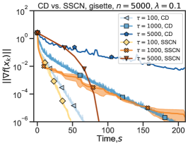
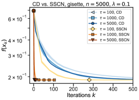
Figure 1: Comparison of CD and SSCN for different constant coordinate schedules, where $\tau$ denotes the dimension of the subspace in the SSCN method. Performance is measured w.r.t. iterations (first column) and time (second column) averaged over three runs for logistic regression with non-convex regularization with $\lambda=0.1$ for the gisette dataset. Experiment details are described in Section 5 and additional plots for the duke and madelon dataset can be found in the Appendix in Fig. 1.

We see in our experiments (Fig. 1), that the combination of second-order information in a coordinate method, as in SSCN, indeed leads to a significant improvement in performance, as compared to the first-order CD. However, while Hanzely et al. (2020) focus on convex objective functions, it has been challenging to show a strict benefit from employing second-order information in coordinate descent methods in non-convex case, which is important for modern applications in machine learning. In this work, we demonstrate that one can obtain strong theoretical convergence guarantees for general, possibly non-convex functions. Toward this goal, we make the following contributions:

• Convergence guarantees: we prove that for non-convex functions, SSCN converges to a stationary point starting from an arbitrary initialization (global convergence), at least with the rate of first-order CD for a rough estimation of the curvature matrix, and with strictly better rates when using the true Hessian (3). The method convergences for an arbitrary selection of $\tau$, and the rate becomes better for larger $\tau$, matching the convergence of the full Cubic Newton for $\tau=n$.

• Sampling schemes: along with the constant sampling (fixed $\tau$), we propose an adaptive theoretical sampling scheme ($\tau_{k}$ grows with $k$) that allows us to prove stronger convergence to a second-order stationary point for SSCN at the full Cubic Newton rate. Thus, this sampling scheme avoids the method to stuck at saddle points which is important for applications. Experimentally, we demonstrate that adaptive sampling does not require to fully sample all coordinates, while preserving the fast rate of convergence for the algorithm.

• Experimentally: Finally, we provide experimental results that verify our theoretical analysis and demonstrate significant speed-ups compared to the classical coordinate descent.

Table 1: Comparison to previous work for non-convex optimization. $\tau_{k}:=\tau(S_{k})$ refers to the adaptive sampling scheme of the main result in Theorem 4.7. And $p_{2}$ is defined as $p_{2}=\frac{\tau(\tau-1)}{n(n-1)}$.

Method	# Coord.	Convergence rate to $\|\nabla f({\bf x})\|\leq\epsilon$	2nd order stationary pt?	Iter. cost (exact step)
Gradient Descent (Nesterov, 2013)	$n$	$\mathcal{O}(k^{-1/2})$	✗	$\mathcal{O}(n)$
Cubic Newton (CR) (Nesterov and Polyak, 2006; Cartis et al., 2011)	$n$	$\mathcal{O}(k^{-2/3})$	✓	$\mathcal{O}(n^{3})$
Stochastic CR (Tripuraneni et al., 2018; Kohler and Lucchi, 2017)	$n$	$\mathcal{O}(k^{-2/3})$	✓	$\mathcal{O}(n^{3})$
Coordinate Descent (Richtárik and Takáč, 2014)	$\tau\leq n$	$\mathcal{O}(k^{-1/2})$	✗	$\mathcal{O}(\tau)$
Random subspace regularized Newton (Fuji et al., 2022)	$\tau\leq n$	$\mathcal{O}(k^{-1/2})$	✗	$\mathcal{O}(\tau^{3})$
This work: Theorem 4.6	$\tau\leq n$	$\mathcal{O}\left(k^{-2/3}+(n(1-p_{2}))^{1/4}k^{-1/2}\right)$	✗	$\mathcal{O}(\tau^{3})$
This work: Theorem 4.7	$\tau_{k}\leq n$	$\mathcal{O}(k^{-2/3})$	✓	$\mathcal{O}(\tau_{k}^{3})$

2 Related work

Newton method and cubic regularization (CR).

The Newton method is the classical optimization algorithm that employs second-order information (the Hessian matrix) about the objective function (Jorge and Stephen, 2006; Nesterov, 2018). Even though the traditional Newton method with a unit step size is effective at handling ill-conditioned problems, it might not achieve global convergence when starting from arbitrary initializations. Therefore, various regularization techniques have been proposed to improve the convergence properties of the Newton method and to ensure the global rates (see Polyak (2007) for a detailed historical overview).

Among these regularization techniques is the well-established cubic regularization of the Newton method, which achieves global complexity bounds that are provably better than those of the gradient descent  (Nesterov and Polyak, 2006). It uses a cubic over-estimator of the objective function as a regularization technique for the computation of a step to minimize the objective function. One limitation of this approach lies in its dependence on calculating the exact minimum of the cubic model. In an alternative approach,  Cartis et al. (2011) introduced the ARC method, which alleviates this demand by allowing for an approximation of the minimizer. Other methods have been proposed to reduce the computational complexity of CR, which we discuss below.

Subsampled/stochastic Newton and CR. For objective functions that have a finite-sum structure, a popular method is to use sub-sampling techniques to approximate the Hessian matrix, such as in Byrd et al. (2011). These techniques have also been adapted to cubic regularization (Kohler and Lucchi, 2017; Tripuraneni et al., 2018) followed by various improvements such as more practical sampling conditions (Wang et al., 2018) or variance reduction (Zhou et al., 2020). We emphasize that there is a notable distinction between our work and these prior works. The latter addresses scenarios involving the sampling of data points, whereas our emphasis lies in the sampling of coordinates. These approaches are therefore orthogonal and could be combined with each other.

Coordinate descent. Coordinate descent methods are particularly useful when dealing with high-dimensional optimization problems, as they allow for efficient optimization by only updating one coordinate at a time, which can be computationally less expensive than updating the entire vector. There is a wide literature focusing on the case where $\tau=1$ with precise convergence rates derived for instance by Nesterov (2012); Richtárik and Takáč (2014). A generalization of CD known as subspace descent  (Kozak et al., 2019) projects the gradient onto a random subspace at each iteration. The rates of convergence of the coordinate descent for non-convex objectives were studied by Patrascu and Necoara (2015).

Subspace Newton. The subspace idea discussed above has also been extended to Newton’s method by Gower et al. (2019) resulting in the update rule ${\bf x}_{k+1}={\bf x}_{k}-\eta{\bf S}_{k}(\nabla_{S}^{2}f({\bf x}_{k}))^{-1}\nabla_{S}f({\bf x}_{k})$, where the gradient and Hessian are computed over a subset of selected coordinates $S$. Finally, Hanzely et al. (2020) extends this idea to cubic regularization, deriving rates of convergence in the more generic case where the objective function $f$ is convex. In contrast, we consider the case where the function $f$ is not necessarily convex. Recently, Fuji et al. (2022) analyzed a randomized subspace version of a (differently regularized) Newton method discussed in Ueda and Yamashita (2010) and obtained convergence to a first-order critical point. An overview of previous works for non-convex optimization can be found in Table 1.

3 Algorithm

3.1 Notation and setting

Our goal is to optimize a bounded below function $f:{\mathbb{R}}^{n}\to{\mathbb{R}}$. We denote $f^{\star}:=\inf_{{\bf x}\in{\mathbb{R}}^{n}}f({\bf x})$. By $\|\cdot\|$ we denote the standard Euclidean norm for vectors and the spectral norm for matrices.

Assumption 3.1.

We assume that $f$ has Lipschitz continuous Hessians with constant $L_{2}\geq 0$, i.e. $\forall{\bf x},{\bf y}\in{\mathbb{R}}^{n}$, it holds $\|\nabla^{2}f({\bf x})-\nabla^{2}f({\bf y})\|\leq L_{2}\|{\bf x}-{\bf y}\|$.

Consequently, we have a global bound for second-order Taylor approximation of $f$, for all ${\bf x},{\bf y}\in{\mathbb{R}}^{n}$:

$$\begin{array}[]{rcl}|f({\bf y})-f({\bf x})-\langle\nabla f({\bf x}),{\bf y}-{\bf x}\rangle-\frac{1}{2}\langle\nabla^{2}f({\bf x})({\bf y}-{\bf x}),{\bf y}-{\bf x}\rangle|&\leq&\frac{L_{2}}{6}\|{\bf y}-{\bf x}\|^{3}.\end{array}$$ (4)

For a given subset of coordinates ${S}\subset[n]:=\{1,\ldots,n\}$ and any vector ${\bf x}\in{\mathbb{R}}^{n}$ we denote by ${\bf x}_{[S]}\in{\mathbb{R}}^{n}$ a vector with nonzero elements whose indices are in $S$ and by ${\bf A}_{[S]}\in{\mathbb{R}}^{n\times n}$ the matrix with nonzero elements whose both rows and columns are in $S$

$$\begin{split}({\bf x}_{[S]})_{i}\overset{\text{def}}{=}\begin{cases}x_{i}\quad&\text{if }i\in S\\ 0\quad&\text{otherwise},\end{cases}\end{split}\qquad\begin{split}({\bf A}_{[S]})_{ij}\overset{\text{def}}{=}\begin{cases}A_{ij}&\quad\text{if }i\in S\text{ and }j\in S\\ 0&\quad\text{otherwise}.\end{cases}\end{split}$$

We also denote the cardinality of set $S$ by $\tau(S):=|S|$. Furthermore, we denote by ${\bf x}|_{S}\in{\mathbb{R}}^{\tau(S)}$ the vector which only contains the entries in ${\bf x}$, which are in $S$. Similarly ${\bf A}|_{S}\in{\mathbb{R}}^{\tau(S)\times\tau(S)}$ contains only the entries ${\bf A}_{ij}$ with $i\in S$ and $j\in S$. Note that $\bm{A}_{[S]}|_{S}\equiv\bm{A}|_{S}$.

3.2 Stochastic subspace cubic newton

Inequality (4) motivates us to introduce the following cubic regularized model, for a given ${\bf x}\in{\mathbb{R}}^{n}$, matrix ${\bf Q}={\bf Q}^{\top}\in{\mathbb{R}}^{n\times n}$, coordinate subset $S\subset[n]$, and regularization parameter $M>0$,

$$\begin{array}[]{rcl}\bar{m}_{{\bf x},{\bf Q},S,M}({\bf h})&:=&f({\bf x})+\langle\nabla f({\bf x}),{\bf h}_{[S]}\rangle+\frac{1}{2}\langle{\bf Q}{\bf h}_{[S]},{\bf h}_{[S]}\rangle+\frac{M}{6}\|{\bf h}_{[S]}\|^{3}\\[7.0pt] &\equiv&f({\bf x})+\langle\nabla f({\bf x})_{[S]},{\bf h}\rangle+\frac{1}{2}\langle{\bf Q}_{[S]}{\bf h},{\bf h}\rangle+\frac{M}{6}\|{\bf h}_{[S]}\|^{3},\qquad{\bf h}\in{\mathbb{R}}^{n}.\end{array}$$

For simplicity and when it is clear from the context, we can omit extra indices, denoting our model simply by $\bar{m}({\bf h})=\bar{m}_{{\bf x},{\bf Q},S,M}({\bf h}):{\mathbb{R}}^{n}\to{\mathbb{R}}$. Then, the next iterate of our method is:

$$\begin{array}[]{rcl}{\bf x}_{k+1}&=&{\bf x}_{k}+\arg\min\limits_{{\bf h}\in{\mathbb{R}}^{n}}\bar{m}_{{\bf x}_{k},{\bf Q}_{k},S_{k},M}({\bf h}),\qquad k\geq 0,\end{array}$$ (5)

where $S_{k}\subset[n]$ are random subspaces of a fixed size $\tau\equiv\tau(S_{k})$, $\tau\in[n]$, so we update the $\tau$ coordinates of ${\bf x}_{k}$ which are in $S_{k}$ in each iteration. Note that for $\tau=n$ we obtain the full cubic Newton step (Nesterov and Polyak, 2006). However, we are interested in choosing $\tau\ll n$, such that the corresponding optimization subproblem (5) can be solved efficiently when $n$ is large.

Remark 3.2.

We note that Eq. (5) is equivalent to the following update rule: ${\bf x}_{k+1}|_{S_{k}}={\bf x}_{k}|_{S_{k}}+\arg\min_{{\bf h}\in{\mathbb{R}}^{\tau}}m_{{\bf x}_{k},{\bf Q}_{k},S_{k},M}({\bf h})$ with a model $m:{\mathbb{R}}^{\tau}\to{\mathbb{R}}$ defined as

$$\begin{array}[]{rcl}m_{{\bf x},{\bf Q},S,M}({\bf h})&:=&f({\bf x})+\langle\nabla f({\bf x})|_{S},{\bf h}\rangle+\frac{1}{2}\langle{\bf Q}|_{S}{\bf h},{\bf h}\rangle+\frac{M}{6}\|{\bf h}\|^{3},\qquad{\bf h}\in{\mathbb{R}}^{\tau}.\end{array}$$ (6)

This update rule implies that in practice we only need to solve a cubic subproblem of dimension $\tau\ll n$. At the same time, in theoretical analysis it is more convenient to work with the initial $\bar{m}$.

1:  Initialization: ${\bf x}_{0}\in{\mathbb{R}}^{n}$, distribution ${\mathcal{D}}$ of random subsets $S\subset[n]$ of size $\tau\equiv\tau(S)$

2:  for $k=0,1,\dots$ do

3:     Sample $S_{k}$ from distribution ${\mathcal{D}}$

4:     Estimate matrix ${\bf Q}_{k}\approx\nabla^{2}f({\bf x}_{k})_{[S_{k}]}$

5:     Set ${\bf x}_{k+1}|_{S_{k}}={\bf x}_{k}|_{S_{k}}+\arg\min_{{\bf h}\in{\mathbb{R}}^{\tau}}m_{{\bf x}_{k},{\bf Q}_{k},S_{k},M_{k}}({\bf h})$, for some $M_{k}>0$

6:  end for

Algorithm 1 SSCN: Stochastic Subspace Cubic Newton

The resulting optimization method is stated in Algorithm 1, where we first sample $S_{k}$ from a chosen distribution ${\mathcal{D}}$, and then perform an update by minimizing our model. Additional details concerning this minimization subproblem will be provided shortly.

In this algorithm, we have a freedom of choosing the matrix ${\bf Q}_{k}$ in every iteration. Even though, we mainly focus on employing the true Hessian $\nabla^{2}f({\bf x}_{k})$ for a selected subset of coordinates, there are several interesting possibilities, that can be also efficiently adapted within our framework.

• Full Hessian matrix: ${\bf Q}_{k}=\nabla^{2}f({\bf x}_{k})_{[S_{k}]}$. Then, our algorithm recovers the SSCN method from Hanzely et al. (2020). This is the most powerful version, which we equip with new strong convergence guarantees, valid for general non-convex objective functions.

• No second-order information: ${\bf Q}_{k}=\bm{0}$. In this case, Algorithm 1 and our analysis recovers the rate of the coordinate descent (CD) method, even though our algorithm is slightly different due to the cubic regularization, which affects the step-size selection: one step becomes ${\bf h}_{k}^{*}=-\eta_{k}\nabla f({\bf x}_{k})|_{S_{k}}\in{\mathbb{R}}^{\tau}$, with $\eta_{k}=\sqrt{2/(M_{k}\|\nabla f({\bf x}_{k})|_{S_{k}}\|)}$. The ability to tackle this extreme case demonstrates the robustness of our iterations: we show that Algorithm 1 works even if the approximation ${\bf Q}_{k}\approx\nabla^{2}f({\bf x}_{k})_{[S_{k}]}$ is not exact.

• Lazy Hessian updates: ${\bf Q}_{k}=\nabla^{2}f({\bf x}_{t})_{[S_{k}]}$, where ${\bf x}_{t}$ is some point from the past, $0\leq t\leq k$. In this approach we use the same Hessian for several steps, which improves the arithmetic complexity of the method Doikov et al. (2023).

• Quasi-Newton updates, such as DFP, BFGS, and L-BFGS (Dennis and Moré, 1977; Nocedal and Wright, 1999). Some recent works combine quasi-Newton methods with the cubic regularization technique, including Kamzolov et al. (2023); Scieur (2024).

• Finite-difference approximation. When second-order information is not directly available, we can approximate the Hessian using only the gradients, as follows: $({\bf Q}_{k})_{ij}=\frac{1}{\delta}(\nabla f({\bf x}_{k}+\delta{\bf e}_{i})-\nabla f({\bf x}_{k}))_{j}$, for $i,j\in S_{k}$, with a possible symmetrization later on. Here, ${\bf e}_{i}$ is the basis vector, and $\delta>0$ is a parameter. Choosing $\delta$ sufficiently small we ensure the rate of the cubic Newton Cartis et al. (2012); Grapiglia et al. (2022); Doikov and Grapiglia (2023).

Complexity of solving the cubic subproblem.

Note that in general, for non-convex functions, the model $\bar{m}({\bf h})$ can be non-convex. However, its global minimum is always well-defined and can be found by standard techniques from linear algebra. One step of our method can be rewritten in the standard form, as in (2): $({\bf x}_{k+1}-{\bf x}_{k})|_{S_{k}}=-\bigl{(}{\bf Q}_{k}|_{S_{k}}+\alpha_{k}{\bf I}\bigr{)}^{-1}\nabla f({\bf x}_{k})|_{S_{k}}$, and the regularization constant $\alpha_{k}$ can be found as a solution to the following univariate concave maximization,

$$\begin{array}[]{c}\max\limits_{\alpha>0}\Bigl{[}-\frac{1}{2}{\langle}\bigl{(}{\bf Q}_{k}|_{S_{k}}+\alpha{\bf I}\bigr{)}^{-1}\nabla f({\bf x}_{k})|_{S_{k}},\nabla f({\bf x}_{k})|_{S_{k}}{\rangle}-\frac{2^{4}\alpha^{3}}{3M_{k}^{2}}\;:\;{\bf Q}_{k}|_{S_{k}}+\alpha{\bf I}\succ\bm{0}\Bigr{]}.\end{array}$$ (7)

It can be done efficiently by means of any one-dimensional procedure (e.g. the binary search or univariate Newton’s method, see also Chapter 7 of Conn et al. (2000) and Section 5 of Nesterov and Polyak (2006)). Then, the complexity of one step is $\mathcal{O}(\tau^{3})$, as for the standard matrix inversion. Cartis et al. (2011) show that one can retain the fast rate with an inexact model minimizer which solves $m({\bf h})$ on a Krylov subspace. The subproblem can also be solved using the gradient descent, as shown by Carmon and Duchi (2019), which means that only Hessian-vector products are required.

4 Convergence analysis

4.1 General convergence rate

First, let us establish a general convergence result for Algorithm 1 when using an arbitrary matrix ${\bf Q}_{k}={\bf Q}_{k}^{\top}\in{\mathbb{R}}^{n\times n}$. To quantify the approximation error, we introduce parameter $\sigma\geq 0$ such that

$$\begin{array}[]{rcl}\|\nabla^{2}f({\bf x}_{k})_{[S_{k}]}-{\bf Q}_{k}\|&\leq&\sigma,\qquad\forall k.\end{array}$$ (8)

Ideally, ${\bf Q}_{k}$ would equal $\nabla^{2}f({\bf x}_{k})_{[S_{k}]}$ (i.e. $\sigma=0$), but our approach accommodates inaccuracies in the Hessian estimation. On the other extreme, when ${\bf Q}_{k}=\bm{0}$ our method should recover the standard rate of the coordinate descent (CD). For that, we have to use an additional assumption.

Assumption 4.1.

Let $f$ have Lipschitz continuous gradient with constant $L_{1}>0$, i.e. $\forall{\bf x},{\bf y}\in{\mathbb{R}}^{n}$, it holds $\|\nabla f({\bf x})-\nabla f({\bf y})\|\leq L_{1}\|{\bf x}-{\bf y}\|$.

By choosing the regularization parameter $M_{k}$ in our cubic model sufficiently large, we can ensure that the following progress condition is satisfied, at each iteration $k\geq 0$:

$$\begin{array}[]{rcl}f({\bf x}_{k}+{\bf h}_{k}^{*})&\leq&\bar{m}_{{\bf x}_{k},{\bf Q}_{k},S_{k},M_{k}}({\bf h}_{k}^{*}).\end{array}$$ (9)

This inequality justifies that our method is monotone (i.e. $f({\bf x}_{k+1})\leq f({\bf x}_{k}))$, and it is crucial for establishing that SSCN can achieve any precision in terms of the gradient norm for any size of a stochastic subspace, and for arbitrary selection of ${\bf Q}_{k}$. All mising proofs are provided in the appendix.

Theorem 4.2.

Let the sequence $\{{\bf x}_{i}\}$ be generated by Algorithm 1 with arbitrary $\bm{Q}_{k}$ satisfying (8), and any fixed $\tau\equiv\tau(S_{k})\in[n]$. Let the regularization parameter at iteration $k\geq 0$ be chosen as

$$\begin{array}[]{rcl}M_{k}&=&2L_{2}+\frac{7^{2}(\sigma+L_{1})^{2}}{2\|\nabla f({\bf x}_{k})_{[S_{k}]}\|}.\end{array}$$ (10)

For a given accuracy level $\varepsilon>0$, assume that $\|\nabla f({\bf x}_{i})\|\geq\varepsilon$, for all $0\leq i\leq K$. Then, it holds

$$\begin{array}[]{rcl}K&\leq&\frac{n}{\tau}\cdot\Bigl{[}\frac{(2+\frac{7^{2}}{3})(\sigma+L_{1})(f({\bf x}_{0})-f^{\star})}{\varepsilon^{2}}+\frac{4L_{2}(f({\bf x}_{0})-f^{\star})}{3(\sigma+L_{1})\varepsilon}\Bigr{]}.\end{array}$$ (11)

4.2 The power of second-order information

In this and the following sections, we assume that we use the exact second-order information, ${\bf Q}_{k}=\nabla^{2}f({\bf x}_{k})_{[S_{k}]}$. In this case, we are able to ensure a faster rate of convergence, thus showing the power of utilizing the second-order information, for general possibly non-convex problems.

Using the model’s optimality (see Section A.1 in the appendix),we can establish that we consistently decrease the objective function at each step, with the following progress.

Lemma 4.3.

For any ${\bf x}_{k}\in{\mathbb{R}}^{n}$ and arbitrary ${S}_{k}\subset[n]$, let ${\bf h}_{k}^{*}=\arg\min_{\bf h}\bar{m}_{{\bf x}_{k},\nabla^{2}f({\bf x}_{k}),S_{k},M}({\bf h})$. Then we have, for any $M\geq L_{2}$,

$$\begin{array}[]{rcl}f({\bf x}_{k})-f({\bf x}_{k+1})&\geq&\frac{M}{12}\|{\bf h}_{k}^{*}\|^{3}.\end{array}$$ (12)

For our refined analysis, we must characterize the distance between the coordinate-sampled gradient $\nabla f({\bf x})_{[S]}$ and the full gradient $\nabla f({\bf x})$, as well as the corresponding distance for the Hessian.

Lemma 4.4.

For any ${\bf x}\in{\mathbb{R}}^{n}$ and any subset $S\subset[n]$, we have

$$\begin{array}[]{rcl}{\mathbb{E}}\|\nabla f({\bf x})-\nabla f({\bf x})_{[S]}\|&\leq&\sqrt{1-\frac{\tau(S)}{n}}\|\nabla f({\bf x})\|,\end{array}$$ (13)

$$\begin{array}[]{rcl}{\mathbb{E}}\|\nabla^{2}f({\bf x})_{[S]}-\nabla^{2}f({\bf x})\|&\leq&\sqrt{1-p_{2}}\|\nabla^{2}f({\bf x})\|_{F},\end{array}$$ (14)

where $p_{2}:=\frac{\tau(S)(\tau(S)-1)}{n(n-1)}$, where $\|\cdot\|_{F}$ is the Frobenius norm of a matrix.

Remark 4.5.

Note that the expectations in Lemma 4.4 are over a subset of coordinates, instead of a subset of datapoints as in Kohler and Lucchi (2017); Tripuraneni et al. (2018); Wang et al. (2018). This distinction implies that the reliance on concentration for sums of i.i.d. random variables, which are used in the latter references, is not applicable in our case. We therefore use a different proof technique that directly exploits the sampling of the coordinates of the gradient and Hessian.

As expected, Lemma 4.4 shows that increasing the sampling size $\tau(S)$ yields more accurate sampled gradients and Hessians. This effect will later be verified experimentally in Section 5 where we will test different coordinate sampling schedules. Notably, the expectation bounds derived in Eqs. (13)-(14) also imply high-probability bounds. We are ready to state our main convergence rate for a fixed coordinate sample size.

Theorem 4.6.

Let the sequence $\{{\bf x}_{i}\}$ be generated by Algorithm 1 with ${\bf Q}_{k}=\nabla^{2}f({\bf x}_{k})_{[S_{k}]}$, and any fixed $\tau\equiv\tau(S_{k})\in[n]$. For a given $\varepsilon>0$, assume that the first $K$ gradients are such that $\|\nabla f({\bf x}_{i})\|\geq\varepsilon,0\leq i\leq K$. Then for a sufficiently large $M\geq L_{2}$, it holds

$$\begin{array}[]{rcl}K&=&\mathcal{O}\Bigl{(}\left[\frac{n}{\tau}\right]^{3/2}\frac{\sqrt{L_{2}}(f({\bf x}_{0})-f^{\star})}{\varepsilon^{3/2}}+n^{1/2}(1-p_{2})^{1/2}\left[\frac{n}{\tau}\right]^{2}\frac{L_{1}(f({\bf x}_{0})-f^{\star}}{\varepsilon^{2}}\Bigr{)}.\end{array}$$ (15)

We see that according to this result, SSCN achieves any desirable accuracy for the gradient norm after a finite number of iterations, starting from an arbitrary initialization ${\bf x}_{0}$. The size of stochastic subspaces $\tau=\tau(S_{k})$ can be arbitrary. Note that $p_{2}=\frac{\tau(\tau-1)}{n(n-1)}$ increases with increasing $\tau$ and we recover the rate of the full Cubic Newton for $\tau=n$. If the cubic subproblem is solved exactly in each iteration (with the cost of $\mathcal{O}(\tau^{3}))$, then the total computational complexity is $\mathcal{O}\Bigl{(}(\tau n)^{3/2}\frac{\sqrt{L_{2}}(f({\bf x}_{0})-f^{\star})}{\varepsilon^{3/2}}+(1-p_{2})^{1/2}\tau n^{5/2}\frac{L_{1}(f({\bf x}_{0})-f^{\star}}{\varepsilon^{2}}\Bigr{)}$. Note that the global computational complexity for CR is $\mathcal{O}\Bigl{(}n^{3}\frac{\sqrt{L_{2}}(f({\bf x}_{0})-f^{\star})}{\varepsilon^{3/2}}\Bigr{)}$. Therefore, we see that SSCN is already strictly better than CR for $\tau(1-p_{2})^{1/2}<(\varepsilon nL_{2})^{1/2}/L_{1}$. Note that in practice we can already observe speed-ups of SSCN for smaller problem dimensions. We also see that the second term in (15) matches the complexity of CD, up to the factor $n^{3/2}(1-p_{2})^{1/2}/\tau$, which tends to $0$ when $\tau\to n$. Lastly, we highlight that the final complexity of SSCN with constant sampling can be taken as the minimum of both (11) and (15), thus achieving the best of these two bounds.

4.3 Adaptive sampling scheme

In the following, we present a scheme to sample the number of coordinates at each iteration that yields even faster convergence to a second-order stationary point up to an arbitrary precision. This scheme is adaptive in the sense that it depends on the gradient and Hessian measured at each iteration. We measure optimality using the standard first and second-order criticality measures $\|\nabla f({\bf x})\|$ and $\lambda_{\min}(\nabla^{2}f({\bf x}))$ (the minimum eigenvalue of the Hessian matrix). To do so, we introduce the following quantity (Nesterov and Polyak, 2006):

$$\begin{array}[]{rcl}\mu({\bf x})&=&\max\left\{\|\nabla f({\bf x})\|^{3/2},\,[-\lambda_{\min}(\nabla^{2}f({\bf x}))]^{3}\right\}.\end{array}$$

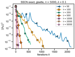
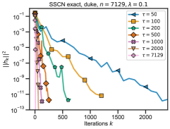
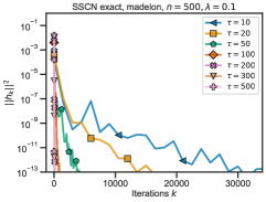
Figure 2: Squared norm of the step ${\bf h}_{k}$ for different constant coordinate schedules for logistic regression with non-convex regularization with $\lambda=0.1$ for three different datasets (left:gisette, center:duke, right:madelon). Note that the y-axis is plotted in log-scale.

Given $\epsilon_{1}>0$ and $\epsilon_{2}>0$, we would like to have

$$\begin{array}[]{rcl}{\mathbb{E}}\|\nabla f({\bf x}_{k})-\nabla f({\bf x}_{k})_{[S_{k}]}\|&\!\!\!\leq\!\!\!&\epsilon_{1},\quad{\mathbb{E}}\|\nabla^{2}f({\bf x}_{k})-\nabla^{2}f({\bf x}_{k})_{[S_{k}]}\|\leq\sqrt{\epsilon_{2}}.\end{array}$$ (16)

Taking into account Lemma 4.4, to ensure (16), it is enough to choose $\tau(S_{k})$ such that

$$\begin{array}[]{rcl}\sqrt{1-\frac{\tau(S_{k})}{n}}&=&\frac{\epsilon_{1}}{\|\nabla f({\bf x}_{k})\|}\qquad\text{and}\qquad\sqrt{1-p_{2}}\;\;=\;\;\frac{\sqrt{\epsilon_{2}}}{\|\nabla^{2}f({\bf x}_{k})\|_{F}}.\end{array}$$

Putting everything together, we obtain the following condition for our adaptive scheme at iteration $k\geq 0$:

$$\begin{array}[]{rcl}\frac{\tau(S_{k})}{n}&\geq&\max\Bigl{\{}1-\frac{\epsilon_{1}^{2}}{\|\nabla f({\bf x}_{k})\|^{2}},\sqrt{1-\frac{\epsilon_{2}}{\|\nabla^{2}f({\bf x}_{k})\|_{F}^{2}}}\Bigr{\}}.\end{array}$$ (17)

Next, we will demonstrate that choosing $\epsilon_{1}=\epsilon_{2}=c_{k-1}\cdot\|{\bf h}_{k-1}^{*}\|^{2}$, for a given sequence $(c_{k})$, allows us to recover the convergence rate of cubic regularization. Importantly, Theorem 4.7 permits the choice of an arbitrary sequence $(c_{k})$ enabling the adjustment of the number of coordinates as a function of the iteration $k$. Section 5 will illustrate that this flexibility leads to an effective strategy, resulting in substantial speed-ups.

Theorem 4.7.

Consider the sequence $\{{\bf x}_{k}\}_{k=0}^{K}$ generated by ${\bf x}_{k+1}={\bf x}_{k}+{\bf h}_{k}^{*}$ where $\tau$ satisfies Eq. (17) with $\epsilon_{1}=\epsilon_{2}=c_{k-1}\cdot\|{\bf h}_{k-1}^{*}\|^{2}$ for some $c_{k-1}>0,\;\forall k=0,\ldots,K$. Let $M\geq L_{2}$. Let $\Delta_{0}=f({\bf x}_{0})-f^{*}$, and define the following constants (dependent on $M$):

$$\begin{array}[]{rcl}C_{M}&=&\left((2M+1)^{3/2}+6\delta^{-3}\max_{i}c_{i}^{3/2}\right)^{-1},\qquad D_{M}\;\;=\;\;\left(\frac{27M^{3}}{8}+\delta^{-3}\max_{i}c_{i}^{3/2}\right)^{-1}.\end{array}$$

Then with probability at least $1-\delta$, we have

$$\begin{array}[]{rcl}\min\limits_{1\leq j\leq K}\mu({\bf x}_{j})&\leq&\frac{1}{K}\left(\frac{6}{M}\max(C_{M}^{-1},D_{M}^{-1})\Delta_{0}+\delta^{-3}c_{-1}^{3/2}\max(3C_{M}^{-1},D_{M}^{-1})\|{\bf h}_{-1}^{*}\|^{3}\right),\end{array}$$

where ${\bf h}_{-1}^{*}$ is such that ${\mathbb{E}}_{[S]}\|\nabla^{2}f({\bf x}_{0})-\nabla^{2}f({\bf x}_{0})_{[S]}\|\leq\sqrt{c_{-1}}\|{\bf h}_{-1}^{*}\|$.

Theorem 4.7 states that Algorithm 1 with an adaptive sampling scheme converges to an $\epsilon$-second-order stationary point at a rate of $\mathcal{O}(\epsilon^{-3/2},\epsilon^{-3})$.

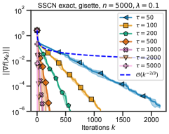
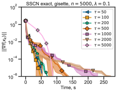
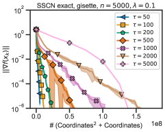
Figure 3: Convergence of different constant coordinate schedules measured w.r.t. iterations (first column), time (second column) and # (Coordinates² + Coordinates) evaluated (third column) averaged over three runs for logistic regression with non-convex regularization with $\lambda=0.1$ for gisette dataset. Same plots for duke madelon, and realsim dataset can be found in Figure 5

A practical scaling rule.

The theoretical result of Theorem 4.7 relies on using Eq. (17) which requires access to the gradient and Hessian norms. We note that one can use the estimates computed over a subset of coordinates $S\subset[n]$. We give further details regarding the validity of this scheme in the Appendix. Alternatively, we have discovered that a less complex schedule produces comparable results. Our starting point is the observation that $\|{\bf h}_{k-1}^{*}\|^{2}$ exhibits exponential growth on most datasets, as illustrated in Figure 2. We posit that this exponential increase allows us to employ a coordinate sampling schedule that also follows an exponential trend. We substantiate the effectiveness of this straightforward approach in Section 5.

Table 2: Overview of the datasets used in the experimental section with non-convex regularizer $\lambda$.

	Type	n	#samples	$\lambda$
gisette	Classification	5.000	6.000	$1e^{-1}$
duke	Classification	7.129	44	$1e^{-1}$
madelon	Classification	500	2.000	$1e^{-1}$

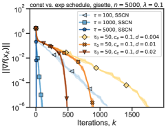
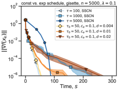
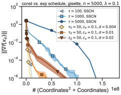
Figure 4: Comparison of constant vs. exponential schedules $\tau(S_{k})=\tau_{0}+c_{e}\exp(dk)$ for different parameters w.r.t. iterations (first column) and time (second column) and # (Coordinates² + Coordinates) evaluated (third column) averaged over three runs for logistic regression with non-convex regularization with $\lambda=0.1$ for the gisette datasets. Same plots for the duke and madelon dataset can be found in the Appendix in Fig. 6.

5 Experiments

We now verify our theoretical results numerically. Due to space limitations, we can only present a fraction of the experiments and refer the reader to the Appendix for the remaining experiments. We ran experiments with a logistic regression loss with a non-convex regularizer $\lambda\cdot\sum_{i=1}^{n}{\bf x}_{i}^{2}/(1+{\bf x}_{i}^{2})$ (Kohler and Lucchi, 2017) where $\lambda>0$ controls the strength of the regularizer. An overview of the three datasets used in our experiments can be found in Table 2. All runs were initialized in the origin at ${\bf x}_{0}=\mathbf{0}$ and all the plots shown in this section are averaged over three runs. The shaded region corresponds to one standard deviation. In the inner loop of Algorithm 1, we solve the subproblem exactly up to a pre-specified tolerance of $1e^{-5}$. We use the exact same subsolver, which is discussed in section 3.3 in Kohler and Lucchi (2017) . The experiments were run on an Apple MacBook Pro with an Apple M1 Pro Chip and 16 GB RAM.

Constant coordinate schedule. In Figure 3 and 5 we plot the convergence of different constant coordinate schedules w.r.t. iterations, time and # (coordinates² + coordinates). We chose the last measure to approximate the efficiency of the coordinate schedule, since the Hessian matrix scales quadratically and the gradient scales linearly with the number of sampled coordinates. As expected, full cubic Newton is the fastest in terms of number of iterations and the fewer coordinates are sampled, the more iterations are required to reach the same gradient norm. However, in terms of average run time and number of evaluated coordinates, we observe that smaller coordinate schedules are faster and more efficient up to some gradient norm for the gisette and duke dataset, where the benefit is more pronounced if the problem is higher dimensional. We note that, even for the smaller madelon dataset, smaller coordinate schedules are more efficient w.r.t # coordinate evaluations until $\|\nabla f({\bf x}_{k})\|\approx 1e^{-1}$. This clearly underscores the potential for substantial computational savings through the utilization of a straightforward approach that samples a fixed number of coordinates. Subsequently, we will explore the performance of this approach in contrast to an adaptive scheme that incrementally increases the number of sampled coordinates.

Constant vs exponential schedule. As discussed earlier, the adaptive sampling scheme presented in Section 4.3 suggests using an exponential schedule to sample coordinates. We compare this schedule to a constant schedule in Figure 4. We observe that for the two high-dimensional datasets gisette and duke, the best constant schedule and the best exponential schedule perform on par both in terms of time and # coordinates evaluated. We conclude that in some cases a simple constant schedule can already perform sufficiently well. However, an exponential schedule might still be more appropriate if one needs a high-accuracy solution.

CD vs SSCN. We compare SSCN to a vanilla randomized coordinate descent (CD) for different constant coordinate schedules. The results are shown in Figure 1. The CD step size $\eta$ was chosen via a line search procedure that guarantees that $f(x_{k+1})-f(x_{k})\geq\frac{\eta}{2}\|\nabla f(x_{k})\|^{2}_{2}$, which is the so-called Armijo condition (Nocedal and Wright, 1999). We evaluate the performance of CD and SSCN by measuring the number of full gradient steps required to converge to a first-order stationary point. For the duke dataset, we observe that CD is extremely fast to converge. Since the per-iteration cost of CD is much lower compared to SSCN, this results in much faster convergence for CD. However, CD converges very slowly to what seems to be a suboptimal solution for the madelon dataset, while for the gisette dataset the fastest schedule is clearly SSCN which only samples $2\%$ of the coordinates. This set of experiments highlights some interesting trade-offs between CD and SSCN. In the case of simpler objective functions, CD demonstrates a clear advantage. However, this advantage can diminish rapidly when dealing with more intricate objective functions where SSCN tends to be more efficient.

6 Conclusion

We analyze the convergence rate of SSCN for the class of twice differentiable non-convex functions. From a theoretical point of view, we demonstrate the convergence of SSCN both with a fixed sampling scheme and an adaptive sampling scheme that recovers the convergence rate of cubic regularization. Furthermore, we have empirically observed that a more straightforward exponential schedule produces favorable results. Overall, our experiments demonstrated that one can sample a fraction of the coordinates while observing fast convergence. This results in significant computational gains compared to the vanilla cubic regularization algorithm. There are various interesting extensions to consider such as the use of importance sampling and combining coordinate sampling with datapoint sampling in the case of finite-sum objective functions.

Appendix

Appendix A Proofs of auxiliary lemmas

A.1 Model optimality

As mentioned earlier, in our analysis, we will assume that each iteration is performed by computing ${\bf h}^{*}_{k}=\arg\min_{{\bf h}\in{\mathbb{R}}^{n}}\bigl{[}\bar{m}({\bf h}):=\bar{m}_{{\bf x}_{k},{\bf Q}_{k},S_{k},M}({\bf h})\bigr{]}$ exactly, and then we set ${\bf x}_{k+1}={\bf x}_{k}+{\bf h}_{k}^{*}$. Of course, in practice the algorithm needs to solve the subproblem only along coordinates in $S_{k}$, which has dimensionality $\tau$. Note that in general (for non-convex objective functions), the model $\bar{m}({\bf h})$ can also be non-convex. However, its global minimum is always well-defined and can be found efficiently by employing standard techniques from linear algebra (see discussion in the end of the previous section). Prior work [Cartis et al., 2011] has shown that it is possible to retain the remarkable properties of the cubic regularization algorithm with an inexact model minimizer. For our purpose, we will simply rely on first-order and second-order optimality, i.e. $\nabla\bar{m}({\bf h}^{*}_{k})=0$ and $\nabla^{2}\bar{m}({\bf h}_{k}^{*})\succeq 0$, which respectively imply:

$$\begin{array}[]{rcl}\nabla f({\bf x}_{k})_{[{S}_{k}]}+{{\bf Q}_{k}}_{[{S}_{k}]}{\bf h}^{*}_{k}+\frac{M}{2}\|{\bf h}^{*}_{k}\|\cdot{\bf h}^{*}_{k}&=&0,\\[10.0pt] {{\bf Q}_{k}}_{[{S}_{k}]}+\frac{M}{2}\|{\bf h}^{*}_{k}\|\cdot{\bf I}+\frac{M}{2\|{\bf h}^{*}_{k}\|}{\bf h}^{*}_{k}({\bf h}^{*}_{k})^{\top}&\succeq&0.\end{array}$$ (18)

Based on these optimality properties, we can establish the following lemmas, which will serve as the foundational bases for our main convergence theorem.

Proposition A.1.

For all global minimizers ${\bf h}^{*}_{k}$ of $\bar{m}({\bf h})=\bar{m}_{{\bf x}_{k},{\bf Q}_{k},{S}_{k},M}({\bf h})$ over ${\mathbb{R}}^{n}$ it holds that

$$\begin{array}[]{rcl}{{\bf Q}_{k}}_{[{S}_{k}]}+\frac{M}{2}\|{\bf h}^{*}_{k}\|\cdot{\bf I}&\succeq&0,\end{array}$$ (19)

where ${\bf I}$ denotes the identity matrix.

Proof.

This proof follows closely the proof of Theorem 3.1 in Cartis et al. [2011]. From the second-order necessary optimality conditions at ${\bf h}^{*}_{k}$ we have

$$\begin{array}[]{rcl}{\langle}\left({{\bf Q}_{k}}_{[{S}_{k}]}+\frac{M}{2}\|{\bf h}^{*}_{k}\|\cdot{\bf I}+\frac{M}{2\|{\bf h}^{*}_{k}\|}{\bf h}^{*}_{k}({\bf h}^{*}_{k})^{\top}\right){\bf w},{\bf w}{\rangle}&\geq&0\end{array}$$

for all vectors ${\bf w}\in{\mathbb{R}}^{n}$.

If ${\bf h}^{*}_{k}=0$, we immediately have the result. Thus, we only need to consider ${\bf h}^{*}_{k}\neq 0$. There are two cases to analyse. Firstly, suppose that ${\langle}{\bf w},{\bf h}^{*}_{k}{\rangle}$ = 0. Then it immediately follows

$$\begin{array}[]{rcl}{\langle}\left({{\bf Q}_{k}}_{[{S}_{k}]}+\frac{M}{2}\|{\bf h}^{*}_{k}\|\cdot{\bf I}\right){\bf w},{\bf w}{\rangle}&\geq&0\qquad\text{for all }{\bf w}\in{\mathbb{R}}^{n}\text{ s.t. }{\langle}{\bf w},{\bf h}^{*}_{k}{\rangle}=0.\end{array}$$ (20)

It remains to consider vectors ${\bf w}$ for which ${\langle}{\bf w},{\bf h}^{*}_{k}{\rangle}\neq 0$. Since ${\bf w}$ and ${\bf h}^{*}_{k}$ are not orthogonal, the line ${\bf h}^{*}_{k}+\alpha{\bf w}$ intersects the ball of radius $\|{\bf h}^{*}_{k}\|$ at two points, ${\bf h}^{*}_{k}$ and ${\bf u}^{*}_{k}\neq{\bf h}^{*}_{k}$, and thus

$$\begin{array}[]{rcl}\|{\bf u}^{*}_{k}\|&=&\|{\bf h}^{*}_{k}\|.\end{array}$$ (21)

Let ${\bf w}^{*}_{k}={\bf u}^{*}_{k}-{\bf h}^{*}_{k}$, and note that ${\bf w}^{*}_{k}$ is parallel to ${\bf w}$, thus ${\bf w}=\beta{\bf w}^{*}_{k}$ for some $\beta\not=0$. Since ${\bf h}^{*}_{k}$ is a global minimizer of $\bar{m}({\bf h})$, we have that

$$\begin{array}[]{rcl}0&\leq&\bar{m}({\bf u}^{*}_{k})-\bar{m}({\bf h}^{*}_{k})\\ \\ &=&\langle\nabla f({\bf x}_{k})_{[S_{k}]},({\bf u}^{*}_{k}-{\bf h}^{*}_{k})\rangle+\frac{1}{2}\langle{{\bf Q}_{k}}_{[{S}_{k}]}{\bf u}^{*}_{k},{\bf u}^{*}_{k}\rangle-\frac{1}{2}\langle{{\bf Q}_{k}}_{[{S}_{k}]}{\bf h}^{*}_{k},{\bf h}^{*}_{k}\rangle\\ \\ &&\qquad+\;\frac{M}{6}(\|{\bf u}^{*}_{k}\|^{3}-\|{\bf h}^{*}_{k}\|^{3})\\ \\ &\overset{\eqref{eq:u_star_norm_=_y_star_norm}}{=}&\langle\nabla f({\bf x}_{k})_{[S_{k}]},({\bf u}^{*}_{k}-{\bf h}^{*}_{k})\rangle+\frac{1}{2}\langle{{\bf Q}_{k}}_{[{S}_{k}]}{\bf u}^{*}_{k},{\bf u}^{*}_{k}\rangle-\frac{1}{2}\langle{{\bf Q}_{k}}_{[{S}_{k}]}{\bf h}^{*}_{k},{\bf h}^{*}_{k}\rangle.\end{array}$$ (22)

But (18) gives that

$$\begin{array}[]{rcl}\langle\nabla f({\bf x}_{k})_{[S_{k}]},({\bf u}^{*}_{k}-{\bf h}^{*}_{k})\rangle&=&\langle{{\bf Q}_{k}}_{[{S}_{k}]}{\bf h}^{*}_{k},({\bf h}^{*}_{k}-{\bf u}^{*}_{k})\rangle+\frac{M}{2}\|{\bf h}^{*}_{k}\|\langle{\bf h}^{*}_{k}-{\bf u}^{*}_{k},{\bf h}^{*}_{k}\rangle.\end{array}$$ (23)

Further note that from (21) it follows that

$$\begin{array}[]{rcl}\langle{\bf h}^{*}_{k}-{\bf u}^{*}_{k},{\bf h}^{*}_{k}\rangle&=&\frac{1}{2}{\langle}{\bf h}^{*}_{k},{\bf h}^{*}_{k}{\rangle}+\frac{1}{2}{\langle}{\bf u}^{*}_{k},{\bf u}^{*}_{k}{\rangle}-{\langle}{\bf u}^{*}_{k},{\bf h}^{*}_{k}{\rangle}\;\;=\;\;\frac{1}{2}\langle{\bf w}^{*}_{k},{\bf w}^{*}_{k}\rangle.\end{array}$$ (24)

Now plugging (24) in (23), and then plugging it in (22) we get

$$\begin{array}[]{rcl}0&\leq&\frac{M}{4}\|{\bf h}^{*}_{k}\|\langle{\bf w}^{*}_{k},{\bf w}^{*}_{k}\rangle+\frac{1}{2}\langle{{\bf Q}_{k}}_{[{S}_{k}]}{\bf h}^{*}_{k},{\bf h}^{*}_{k}\rangle-\langle{{\bf Q}_{k}}_{[{S}_{k}]}{\bf h}^{*}_{k},{\bf u}^{*}_{k}\rangle\\ \\ &&\qquad+\;\frac{1}{2}\langle{{\bf Q}_{k}}_{[{S}_{k}]}{\bf u}^{*}_{k},{\bf u}^{*}_{k}\rangle\\ \\ &=&\frac{M}{4}\|{\bf h}^{*}_{k}\|\langle{\bf w}^{*}_{k},{\bf w}^{*}_{k}\rangle+\frac{1}{2}\langle{{\bf Q}_{k}}_{[{S}_{k}]}({\bf u}^{*}_{k}-{\bf h}^{*}_{k}),({\bf u}^{*}_{k}-{\bf h}^{*}_{k})\rangle\\ \\ &\overset{{\bf w}_{k}^{*}={\bf u}_{k}^{*}-{\bf h}_{k}^{*}}{=}&\frac{1}{2}\left\langle\left({{\bf Q}_{k}}_{[{S}_{k}]}+\frac{M}{2}\|{\bf h}^{*}_{k}\|\cdot{\bf I}\right)({\bf u}^{*}_{k}-{\bf h}^{*}_{k}),({\bf u}^{*}_{k}-{\bf h}^{*}_{k})\right\rangle\\ \\ &=&\frac{1}{2\beta}\left\langle\left({{\bf Q}_{k}}_{[{S}_{k}]}+\frac{M}{2}\|{\bf h}^{*}_{k}\|\cdot{\bf I}\right){\bf w},{\bf w}\right\rangle.\end{array}$$ (25)

Therefore, it holds for any ${\bf w}\in{\mathbb{R}}^{n}$ such that ${\langle}{\bf w},{\bf h}^{*}_{k}{\rangle}\neq 0$. Finally we can conclude from (20) and (25) that

$$\begin{array}[]{rcl}{{\bf Q}_{k}}_{[{S}_{k}]}+\frac{M}{2}\|{\bf h}^{*}_{k}\|\cdot{\bf I}&\succeq&0,\end{array}$$

which completes the proof. ∎

Lemma A.2.

For all global minimizers ${\bf h}^{*}_{k}$ of $\bar{m}({\bf h})=\bar{m}_{{\bf x}_{k},{\bf Q}_{k},{S}_{k},M}({\bf h})$ over ${\mathbb{R}}^{n}$ it holds that

$$\begin{array}[]{rcl}\langle\nabla f({\bf x}_{k})_{[{S}_{k}]},{\bf h}_{k}^{*}\rangle&\leq&0.\end{array}$$ (26)

Proof.

Multiplying (19) twice with ${\bf h}_{k}^{*}$ and multiplying (18) once with ${\bf h}_{k}^{*}$ we get

$$\begin{array}[]{rcl}\langle{{\bf Q}_{k}}_{[{S}_{k}]}{\bf h}_{k}^{*},{\bf h}_{k}^{*}\rangle+\frac{M}{2}\|{\bf h}_{k}^{*}\|^{3}&\geq&0,\\ \\ \langle\nabla f({\bf x}_{k})_{[S_{k}]},{\bf h}_{k}^{*}\rangle+{{\bf Q}_{k}}_{[{S}_{k}]}{\bf h}_{k}^{*},{\bf h}_{k}^{*}\rangle+\frac{M}{2}\|{\bf h}_{k}^{*}\|^{3}&=&0.\end{array}$$

∎

Note that (19) is a stronger version of the standard second-order optimality condition (18), which takes additionally into account that ${\bf h}^{*}$ is a global minimum.

See 4.3

Proof Lemma 4.3.

By 3.1,we have for all ${\bf x},{\bf y}\in{\mathbb{R}}^{n}$:

$$\begin{array}[]{rcl}|f({\bf y})-f({\bf x})-\langle\nabla f({\bf x}),{\bf y}-{\bf x}\rangle-\frac{1}{2}\langle\nabla^{2}f({\bf x})({\bf y}-{\bf x}),{\bf y}-{\bf x}\rangle|&\leq&\frac{L_{2}}{6}\|{\bf y}-{\bf x}\|^{3}.\end{array}$$

This implies that,

$$\begin{array}[]{rcl}f({\bf x}_{k+1})&\leq&f({\bf x}_{k})+\langle\nabla f({\bf x}_{k}),{\bf h}_{k}^{*}\rangle+\frac{1}{2}\langle\nabla^{2}f({\bf x}_{k}){\bf h}_{k}^{*},{\bf h}_{k}^{*}\rangle+\frac{L_{2}}{6}\|{\bf h}_{k}^{*}\|^{3}\\ \\ &\leq&f({\bf x}_{k})+\langle\nabla f({\bf x}_{k}),{\bf h}_{k}^{*}\rangle+\frac{1}{2}\langle\nabla^{2}f({\bf x}_{k}){\bf h}_{k}^{*},{\bf h}_{k}^{*}\rangle+\frac{M}{6}\|{\bf h}_{k}^{*}\|^{3}\\ \\ &=&f({\bf x}_{k})+\langle\nabla f({\bf x}_{k})_{[S_{k}]},{\bf h}_{k}^{*}\rangle+\frac{1}{2}\langle\nabla^{2}f({\bf x}_{k})_{[S_{k}]}{\bf h}_{k}^{*},{\bf h}_{k}^{*}\rangle+\frac{M}{6}\|{\bf h}_{k}^{*}\|^{3}\\ \\ &=&\bar{m}_{{\bf x}_{k},\nabla^{2}f({\bf x}_{k}),S_{k},M}({\bf h}_{k}^{*}),\end{array}$$ (27)

where we used $M\geq L_{2}$ in the second inequality.

By first-order optimality of the cubic model, recall that

$$\begin{array}[]{rcl}\nabla f({\bf x}_{k})_{[{S}_{k}]}+\nabla^{2}f({\bf x}_{k})_{[{S}_{k}]}{\bf h}^{*}_{k}+\frac{M}{2}\|{\bf h}^{*}_{k}\|\cdot{\bf h}^{*}_{k}&=&0.\end{array}$$

Taking the inner product with ${\bf h}^{*}_{k}$, we obtain

$$\begin{array}[]{rcl}\langle\nabla^{2}f({\bf x}_{k})_{[{S}_{k}]}{\bf h}^{*}_{k},{\bf h}^{*}_{k}\rangle&=&-\langle\nabla f({\bf x}_{k})_{[{S}_{k}]},{\bf h}^{*}_{k}\rangle-\frac{M}{2}\|{\bf h}^{*}_{k}\|^{3}.\end{array}$$ (28)

Combining Eq. (27) and (28), we obtain

$$\begin{array}[]{rcl}f({\bf x}_{k+1})-f({\bf x}_{k})&\leq&\frac{1}{2}\langle\nabla f({\bf x}_{k})_{[S_{k}]},{\bf h}_{k}^{*}\rangle-\frac{M}{12}\|{\bf h}_{k}^{*}\|^{3}\\ \\ &\leq&-\frac{M}{12}\|{\bf h}_{k}^{*}\|^{3},\end{array}$$

where the last inequality holds since $\langle\nabla f({\bf x}_{k})_{[{S}_{k}]},{\bf h}_{k}^{*}\rangle\leq 0$ by Eq. (26). ∎

Appendix B Convergence of a fixed sampling scheme

In this section, we assume that in each iteration we sample a coordinate subspace $S_{k}$ of the same fixed sample size $\tau(S_{k})\equiv\tau\in[n]$. We establish the global convergence rates for our method, for an arbitrary initialization ${\bf x}_{0}$.

B.1 General convergence rate

Let us prove our general result that allows for an approximate matrix ${\bf Q}\approx\nabla^{2}f({\bf x}_{k})_{[S_{k}]}$.

See 4.2

Proof.

First, we want to choose $M_{k}>0$ such that the following progress condition is satisfied:

$$\begin{array}[]{rcl}f({\bf x}_{k}+{\bf h}_{k}^{*})&\leq&\bar{m}_{{\bf x}_{k},{\bf Q}_{k},S_{k},M_{k}}({\bf h}_{k}^{*}).\end{array}$$ (29)

We can ensure that this condition holds for a sufficiently large value of $M_{k}$. Indeed, by Lipschitzness of the Hessian, we have

$$\begin{array}[]{rcl}f({\bf x}_{k}+{\bf h}_{k}^{*})&\leq&f({\bf x}_{k})+{\langle}\nabla f({\bf x}_{k})_{[S_{k}]}{\bf h}_{k}^{*}{\rangle}+\frac{1}{2}{\langle}\nabla^{2}f({\bf x}_{k})_{[S_{k}]}{\bf h}_{k}^{*},{\bf h}_{k}^{*}{\rangle}+\frac{L_{2}}{6}\|{\bf h}_{k}^{*}\|^{3}\\ \\ &=&\bar{m}_{{\bf x}_{k},{\bf Q}_{k},S_{k},M_{k}}({\bf h}_{k}^{*})+\frac{1}{2}{\langle}(\nabla^{2}f({\bf x}_{k})_{[S_{k}]}-\bm{Q}_{k}){\bf h}_{k}^{*},{\bf h}_{k}^{*}{\rangle}+\frac{L_{2}-M_{k}}{6}\|{\bf h}_{k}^{*}\|^{3}\\ \\ &\overset{\eqref{SigmaDef}}{\leq}&\bar{m}_{{\bf x}_{k},{\bf Q}_{k},S_{k},M_{k}}({\bf h}_{k}^{*})+\frac{\sigma}{2}\|{\bf h}_{k}^{*}\|^{2}+\frac{L_{2}-M_{k}}{6}\|{\bf h}_{k}^{*}\|^{3},\end{array}$$

and to satisfy (9), it is sufficient to have

$$\begin{array}[]{rcl}\frac{M_{k}}{6}\|{\bf h}_{k}^{*}\|^{3}&\geq&\frac{\sigma}{2}\|{\bf h}_{k}^{*}\|^{2}+\frac{L_{2}}{6}\|{\bf h}_{k}^{*}\|^{3}.\end{array}$$ (30)

Note that the stationary condition for ${\bf h}_{k}^{*}$ gives

$$\begin{array}[]{rcl}\nabla f({\bf x}_{k})_{[S_{k}]}+\bm{Q}_{k}{\bf h}_{k}^{*}+\frac{M_{k}}{2}\|{\bf h}_{k}^{*}\|{\bf h}_{k}^{*}&=&0,\\ \\ \bm{Q}_{k}+\frac{M_{k}}{2}\bm{I}&\succeq&0.\end{array}$$ (31)

Then, observe that

$$\bm{Q}_{k}\overset{\eqref{SigmaDef}}{\preceq}\sigma\bm{I}+\nabla^{2}f({\bf x}_{k})_{[S_{k}]}\;\;\preceq\;\;(\sigma+L_{1})\bm{I},$$ (32)

where the second inequality is due to Assumption 4.1.
Denoting $r:=\|{\bf h}_{k}^{*}\|$, we get

$$\begin{array}[]{rcl}\|\nabla f({\bf x}_{k})_{[S_{k}]}\|^{2}&\overset{\eqref{QStatCond}}{=}&{\langle}(\bm{Q}_{k}+\frac{M_{k}r}{2}\bm{I})^{2}{\bf h}_{k}^{*},{\bf h}_{k}^{*}{\rangle}\;\;\overset{\eqref{eq:bound_Q}}{\leq}\;\;(\sigma+L_{1}+\frac{M_{k}r}{2})^{2}r^{2}.\end{array}$$

Hence,

$$\begin{array}[]{rcl}\frac{M_{k}}{2}r^{2}+(\sigma+L_{1})r&\geq&\|\nabla f({\bf x}_{k})_{[S_{k}]}\|.\end{array}$$ (33)

Resolving the quadratic equation, we conclude from (33) that

$$\begin{array}[]{rcl}M_{k}\|{\bf h}_{k}^{*}\|&=&M_{k}r\;\;\overset{\eqref{RIneq}}{\geq}\;\;\sqrt{(\sigma+L_{1})^{2}+2M_{k}\|\nabla f({\bf x}_{k})_{[S_{k}]}\|}-\sigma-L_{1}.\end{array}$$ (34)

Therefore, we can estimate the left hand side in (30) as follows,

$$\begin{array}[]{rcl}\frac{M_{k}}{6}\|{\bf h}_{k}^{*}\|^{3}&=&\frac{M_{k}}{12}\|{\bf h}_{k}^{*}\|^{3}+\frac{M_{k}}{12}\|{\bf h}_{k}^{*}\|^{3}\\ \\ &\geq&\frac{\sqrt{(\sigma+L_{1})^{2}+2M_{k}\|\nabla f({\bf x}_{k})_{[S_{k}]}\|}-\sigma-L_{1}}{12}\|{\bf h}_{k}^{*}\|^{2}+\frac{M_{k}}{12}\|{\bf h}_{k}^{*}\|^{3},\end{array}$$

and to ensure the inequality in (29), it is sufficient to choose any $M_{k}\geq 2L_{2}+\frac{(7\sigma+L_{1})^{2}}{2\|\nabla f({\bf x}_{k})_{[S_{k}]}\|}$. Let us make the following simple choice:

$$\boxed{\begin{array}[]{rcl}M_{k}&:=&2L_{2}+\frac{7^{2}(\sigma+L_{1})^{2}}{2\|\nabla f({\bf x}_{k})_{[S_{k}]}\|}.\end{array}}$$ (35)

Note that without loss of generality we assume that $\|\nabla f({\bf x}_{k})_{[S_{k}]}\|>0$. Otherwise, the algorithm simply does not move for the current step, since it appears to be already in a local optimum in the sampled subspace.

Therefore, for this choice of $M_{k}$, we have established, for arbitrary ${\bf y}\in{\mathbb{R}}^{n}$:

$$\begin{array}[]{rcl}f({\bf x}_{k+1})&\leq&\bar{m}_{{\bf x}_{k},{\bf Q}_{k},S_{k},M_{k}}({\bf h}_{k}^{*})\;\;\leq\;\;\bar{m}_{{\bf x}_{k},{\bf Q}_{k},S_{k},M_{k}}({\bf y}-{\bf x}_{k}),\end{array}$$

where the last inequality holds since ${\bf h}_{k}^{*}$ is a global minimum of the model. Hence, for any ${\bf y}\in{\mathbb{R}}^{n}$, we have:

$$\begin{array}[]{rcl}f({\bf x}_{k+1})&\leq&f({\bf x}_{k})+{\langle}\nabla f({\bf x}_{k})_{[S_{k}]},{\bf y}-{\bf x}_{k}{\rangle}+\frac{1}{2}{\langle}{{\bf Q}_{k}}_{[S_{k}]}({\bf y}-{\bf x}_{k}),{\bf y}-{\bf x}_{k}{\rangle}+\frac{M_{k}}{6}\|{\bf y}-{\bf x}_{k}\|^{3}\\ \\ &\overset{\eqref{eq:bound_Q}}{\leq}&f({\bf x}_{k})+{\langle}\nabla f({\bf x}_{k})_{[S_{k}]},{\bf y}-{\bf x}_{k}{\rangle}+\frac{\sigma+L_{1}}{2}\|{\bf y}-{\bf x}_{k}\|^{2}+\frac{M_{k}}{6}\|{\bf y}-{\bf x}_{k}\|^{3}.\end{array}$$

Let us take ${\bf y}:={\bf x}_{k}-\alpha\nabla f({\bf x}_{k})_{[S_{k}]}$ (the coordinated descent step), with some $\alpha>0$. Then,

$$\begin{array}[]{rcl}f({\bf x}_{k+1})&\leq&f({\bf x}_{k})-\alpha\|\nabla f({\bf x}_{k})_{[S_{k}]}\|^{2}+\frac{\alpha^{2}(\sigma+L_{1})}{2}\|\nabla f({\bf x}_{k})_{[S_{k}]}\|^{2}+\frac{\alpha^{3}M_{k}}{6}\|\nabla f({\bf x}_{k})_{[S_{k}]}\|^{3},\end{array}$$

or, rearranging the terms,

$$\begin{array}[]{rcl}f({\bf x}_{k})-f({\bf x}_{k+1})&\geq&\alpha\|\nabla f({\bf x}_{k})_{[S_{k}]}\|^{2}\cdot\Bigl{(}1-\frac{\alpha(\sigma+L_{1})}{2}-\frac{\alpha^{2}M_{k}}{6}\|\nabla f({\bf x}_{k})_{[S_{k}]}\|\Bigr{)}.\end{array}$$

Note that $\alpha>0$ is an arbitrary stepsize. We choose it in a way to have

$$\begin{array}[]{rcl}1-\frac{\alpha(\sigma+L_{1})}{2}-\frac{\alpha^{2}M_{k}}{6}\|\nabla f({\bf x}_{k})_{[S_{k}]}\|&=&\frac{1}{2},\end{array}$$

which is achieved by finding the positive root of the quadratic equation. We obtain, denoting $g:=\|\nabla f({\bf x}_{k})_{[S_{k}]}\|$ and $\beta:=L_{1}+\sigma$:

$$\begin{array}[]{rcl}\alpha&:=&\frac{-\beta+\sqrt{\beta^{2}+\frac{4}{3}M_{k}g}}{\frac{2}{3}M_{k}g}\;\;=\;\;\frac{3\beta}{2M_{k}g}\cdot\Bigl{(}\sqrt{1+\frac{4M_{k}}{3\beta^{2}}g}\;-\;1\Bigr{)}\\ \\ &=&\frac{3\beta}{2M_{k}g}\cdot\frac{1+\frac{4M_{k}}{3\beta^{2}}g-1}{\sqrt{1+\frac{4M_{k}}{3\beta^{2}}g}\;+\;1}\;\;=\;\;\frac{2}{\beta}\cdot\frac{1}{\sqrt{1+\frac{4M_{k}}{3\beta^{2}}g}\;+\;1}\\ \\ &\geq&\frac{2}{\beta}\cdot\frac{1}{2+\frac{2M_{k}}{3\beta^{2}}g},\end{array}$$

where in the last bound we used the inequality $\sqrt{1+t}\leq 1+\frac{t}{2}$, valid for $t\geq 0$.

Thus, we obtain the following progress for one step of our method:

$$\begin{array}[]{rcl}f({\bf x}_{k})-f({\bf x}_{k+1})&\geq&\frac{1}{\beta}\|\nabla f({\bf x}_{k})_{[S_{k}]}\|^{2}\cdot\frac{1}{2+\frac{2M_{k}}{3\beta^{2}}\|\nabla f({\bf x}_{k})_{[S_{k}]}\|}\\ \\ &=&\frac{1}{2\beta}\frac{\|\nabla f({\bf x}_{k})_{[S_{k}]}\|^{2}}{1+\frac{M_{k}}{3\beta^{2}}\|\nabla f({\bf x}_{k})_{[S_{k}]}\|}\\ \\ &\overset{\eqref{M_k_Q_Choice}}{=}&\frac{1}{2\beta}\frac{\|\nabla f({\bf x}_{k})_{[S_{k}]}\|^{2}}{1+\frac{7^{2}}{6}+\frac{2L_{2}}{3\beta^{2}}\|\nabla f({\bf x}_{k})_{[S_{k}]}\|}\\ \\ &\geq&\frac{1}{2\beta}\frac{\|\nabla f({\bf x}_{k})_{[S_{k}]}\|^{2}}{1+\frac{7^{2}}{6}+\frac{2L_{2}}{3\beta^{2}}\|\nabla f({\bf x}_{k})\|},\end{array}$$

where the last inequality holds due to the trivial observation,

$$\begin{array}[]{rcl}\|\nabla f({\bf x}_{k})_{[S_{k}]}\|^{2}&=&\sum\limits_{i\in S_{k}}(\nabla f({\bf x}_{k}))_{i}^{2}\;\;\leq\;\;\sum\limits_{i=1}^{n}(\nabla f({\bf x}_{k}))_{i}^{2}\;\;=\;\;\|\nabla f({\bf x}_{k})\|^{2}.\end{array}$$

Taking the expectation w.r.t. $S_{k}$, we get

$$\begin{array}[]{rcl}{\mathbb{E}}_{S_{k}}\Bigl{[}f({\bf x}_{k})-f({\bf x}_{k+1})\Bigr{]}&\geq&\frac{1}{2\beta}\frac{{\mathbb{E}}_{S_{k}}\|\nabla f({\bf x}_{k})_{[S_{k}]}\|^{2}}{1+\frac{7^{2}}{6}+\frac{2L_{2}}{3\beta^{2}}\|\nabla f({\bf x}_{k})\|}\;\;=\;\;\frac{1}{2\beta}\frac{(\frac{\tau}{n})\|\nabla f({\bf x}_{k})\|^{2}}{1+\frac{7^{2}}{6}+\frac{2L_{2}}{3\beta^{2}}\|\nabla f({\bf x}_{k})\|}.\end{array}$$

The last equality holds because

$${\mathbb{E}}_{S}\|\nabla f({\bf x}_{k})_{[S_{k}]}\|^{2}=\sum\limits_{i=1}^{n}{\mathbb{E}}_{S}(\nabla f({\bf x}_{k})^{(i)}1_{i\in S_{k}})^{2}=\frac{\tau(S_{k})}{n}\|\nabla f({\bf x}_{k})\|^{2},$$ (36)

where we used ${\mathbb{E}}_{S}[(1_{i\in S})^{2}]={\mathbb{E}}_{S}[(1_{i\in S})]=\frac{\tau(S)}{n}$.

Assuming that $\|\nabla f({\bf x}_{k})\|\geq\varepsilon$ and using monotonicity of the last expression w.r.t $\|\nabla f({\bf x}_{k})\|$, we obtain

$$\begin{array}[]{rcl}{\mathbb{E}}_{S_{k}}\Bigl{[}f({\bf x}_{k})-f({\bf x}_{k+1})\Bigr{]}&\geq&\frac{(\frac{\tau}{n})\varepsilon^{2}}{2\beta(1+\frac{7^{2}}{6})+\frac{4L_{2}}{3\beta}\varepsilon}.\end{array}$$

Taking the full expectation and telescoping this bound for $K$ iterations, we obtain

$$\begin{array}[]{rcl}f({\bf x}_{0})-f^{\star}&\geq&f({\bf x}_{0})-{\mathbb{E}}f({\bf x}_{K})\;\;\geq\;\;\frac{(\frac{\tau}{n})\varepsilon^{2}K}{2\beta(1+\frac{7^{2}}{6})+\frac{4L_{2}}{3\beta}\varepsilon},\end{array}$$

which leads to the following global complexity:

$$\begin{array}[]{rcl}K&\leq&\frac{n}{\tau}\cdot\frac{2(1+\frac{7^{2}}{6})\beta(f({\bf x}_{0})-f^{\star})}{\varepsilon^{2}}+\frac{n}{\tau}\cdot\frac{4L_{2}(f({\bf x}_{0})-f^{\star})}{3\beta\varepsilon}.\end{array}$$

∎

B.2 The power of second-order information

In this section, we use exact second-order information, ${\bf Q}_{k}=\nabla^{2}f({\bf x}_{k})_{[S_{k}]}$. We show that in this case, it is possible to prove better convergence rates that interpolate between CD and the full Cubic Newton method.

By Lemma C.1, we have that

$$\begin{array}[]{rcl}{\mathbb{E}}_{S}\|\nabla f({\bf x})-\nabla f({\bf x})_{[S]}\|&\leq&\sqrt{1-\frac{\tau}{n}}\|\nabla f({\bf x})\|.\end{array}$$ (37)

And from the proof of Lemma C.2, we get

$$\begin{array}[]{rcl}{\mathbb{E}}_{S}\|\nabla^{2}f({\bf x})-\nabla^{2}f({\bf x})_{[S]}\|^{2}_{2}&\leq&(1-p_{2})\|\nabla^{2}f({\bf x})\|_{F}^{2},\end{array}$$ (38)

where $p_{2}=\frac{\tau(\tau-1)}{n(n-1)}$.

Let us repeat the analysis of one step of our method, employing bounds (37) and (38) directly. The goal is to refine Lemma C.4. We fix ${\bf x}_{k}$ and consider one step of the method:

$$\begin{array}[]{rcl}{\bf h}_{k}^{*}&=&\text{argmin}_{{\bf h}}m_{3}({\bf h};{\bf x}_{k},S_{k})\end{array}$$ (39)

for an arbitrary $S_{k}\subset[n]$ and $M\geq L_{2}$. Then by first order optimality of $h_{k}^{*}$, the new gradient norm is bounded as

$$\begin{array}[]{rcl}\|\nabla f({\bf x}_{k}+{\bf h}_{k}^{*})\|&\leq&\|\nabla f({\bf x}_{k})+\nabla^{2}f({\bf x}_{k}){\bf h}_{k}^{*}\|+\frac{L_{2}}{2}\|{\bf h}_{k}^{*}\|^{2}\\ \\ &\leq&\|\nabla f({\bf x}_{k})-\nabla f({\bf x}_{k})_{[S_{k}]}\|+\|(\nabla^{2}f({\bf x}_{k})-\nabla^{2}f({\bf x}_{k})_{[S_{k}]}){\bf h}_{k}^{*}\|\\ \\ &&\quad+\;\frac{L_{2}}{2}\|{\bf h}_{k}^{*}\|^{2}+\|\nabla f({\bf x}_{k})_{[S_{k}]}+\nabla^{2}f({\bf x}_{k})_{[S_{k}]}{\bf h}_{k}^{*}\|\\ \\ &\overset{\eqref{eq:first_order_optimality}}{=}&\|\nabla f({\bf x}_{k})-\nabla f({\bf x}_{k})_{[S_{k}]}\|+\|(\nabla^{2}f({\bf x}_{k})-\nabla^{2}f({\bf x}_{k})_{[S_{k}]}){\bf h}_{k}^{*}\|\\ \\ &&\quad+\;\frac{L_{2}+M}{2}\|{\bf h}_{k}^{*}\|^{2}\\ \\ &\leq&\|\nabla f({\bf x}_{k})-\nabla f({\bf x}_{k})_{[S_{k}]}\|+\|\nabla^{2}f({\bf x}_{k})-\nabla^{2}f({\bf x}_{k})_{[S_{k}]}\|\cdot\|{\bf h}_{k}^{*}\|\\ \\ &&\quad+\;\frac{L_{2}+M}{2}\|{\bf h}_{k}^{*}\|^{2}.\end{array}$$

Now, we take (the full) expectation ${\mathbb{E}}_{S}[\cdot]$ and use the Cauchy-Schwartz inequality for random variables:

$$\begin{array}[]{rcl}{\mathbb{E}}_{S}\|\nabla f({\bf x}_{k}+{\bf h}_{k}^{*})\|&\leq&{\mathbb{E}}_{S}\|\nabla f({\bf x}_{k})-\nabla f({\bf x}_{k})_{[S_{k}]}\|\\ \\ &&\qquad+\;\sqrt{{\mathbb{E}}\bigl{[}\|\nabla^{2}f({\bf x}_{k})-\nabla^{2}f({\bf x}_{k})_{[S_{k}]}\|^{2}\bigr{]}\cdot{\mathbb{E}}\bigl{[}\|{\bf h}_{k}^{*}\|^{2}\bigr{]}}\\ \\ &&\qquad+\;\frac{L_{2}+M}{2}{\mathbb{E}}_{S}[\|{\bf h}_{k}^{*}\|^{2}]\\ \\ &\overset{\eqref{GradBound},\eqref{HessBound}}{\leq}&\sqrt{1-\frac{\tau}{n}}\cdot{\mathbb{E}}_{S}\|\nabla f({\bf x}_{k})\|\\ \\ &&\qquad+\;\sqrt{(1-p_{2}){\mathbb{E}}_{S}\|\nabla^{2}f({\bf x}_{k})\|_{F}^{2}\cdot{\mathbb{E}}_{S}[\|{\bf h}_{k}^{*}\|^{2}]}+\frac{L_{2}+M}{2}{\mathbb{E}}_{S}[\|{\bf h}_{k}^{*}\|^{2}]\\ \\ &\overset{(*)}{\leq}&\sqrt{1-\frac{\tau}{n}}\cdot{\mathbb{E}}_{S}\|\nabla f({\bf x}_{k})\|+\frac{(1-p_{2}){\mathbb{E}}_{S}\|\nabla^{2}f({\bf x}_{k})\|_{F}^{2}}{2M}+\frac{L_{2}+2M}{2}{\mathbb{E}}_{S}[\|{\bf h}_{k}^{*}\|^{2}]\\ \\ &\leq&\sqrt{1-\frac{\tau}{n}}\cdot{\mathbb{E}}_{S}\|\nabla f({\bf x}_{k})\|+\frac{(1-p_{2}){\mathbb{E}}_{S}\|\nabla^{2}f({\bf x}_{k})\|_{F}^{2}}{2M}+\frac{3M}{2}{\mathbb{E}}_{S}[\|{\bf h}_{k}^{*}\|^{2}],\end{array}$$

where we used Young’s inequality in $(*)$.

Since the function $g(x)=x^{3/2},x\geq 0$ is convex, we have, for an arbitrary $\lambda\in(0,1)$, and $a,b\geq 0$:

$$\begin{array}[]{rcl}(a+b)^{3/2}&=&\frac{1}{\lambda^{3/2}}\Bigl{(}\lambda a+(1-\lambda)\bigl{[}\frac{\lambda}{1-\lambda}(b)\bigr{]}\Bigr{)}^{3/2}\\ \\ &\leq&\frac{1}{\lambda^{1/2}}a^{3/2}+\frac{1}{(1-\lambda)^{1/2}}b^{3/2}.\end{array}$$ (40)

Let us fix some $\lambda_{*}\in(0,1)$, and use inequality (40) with $\lambda:=\lambda_{*}\in(0,1)$, obtaining:

$$\begin{array}[]{rcl}&&\!\!\!\!\!\!\!\!\!\!\!\!\!\!\!({\mathbb{E}}_{S}\|\nabla f({\bf x}_{k}+{\bf h}_{k}^{*})\|)^{3/2}\\ \\ &\leq&\frac{1}{\lambda_{*}^{1/2}}\bigl{[}1-\frac{\tau}{n}\bigr{]}^{3/4}({\mathbb{E}}_{S}\|\nabla f({\bf x}_{k})\|)^{3/2}+\bigl{[}\frac{1}{1-\lambda_{*}}\bigr{]}^{1/2}\cdot\Bigl{(}\frac{(1-p_{2}){\mathbb{E}}_{S}\|\nabla^{2}f({\bf x}_{k})\|_{F}^{2}}{2M}+\frac{3M}{2}{\mathbb{E}}_{S}[\|{\bf h}_{k}^{*}\|^{2}]\Bigr{)}^{3/2}\\ \\ &\leq&\frac{1}{\lambda_{*}^{1/2}}\bigl{[}1-\frac{\tau}{n}\bigr{]}^{3/4}({\mathbb{E}}_{S}\|\nabla f({\bf x}_{k})\|)^{3/2}+\bigl{[}\frac{2}{1-\lambda_{*}}\bigr{]}^{1/2}\cdot\frac{(1-p_{2})^{3/2}}{(2M)^{3/2}}{\mathbb{E}}_{S}\|\nabla^{2}f({\bf x}_{k})\|_{F}^{3}\\ \\ &&\qquad+\;\bigl{[}\frac{2}{1-\lambda_{*}}\bigr{]}^{1/2}\bigl{[}\frac{3M}{2}\bigr{]}^{3/2}{\mathbb{E}}_{S}[\|{\bf h}_{k}^{*}\|^{3}]\end{array}$$

where in the last inequality we used (40) again, but with $\lambda:=\frac{1}{2}$, as well as Jensen’s inequality for the expectation. Hence, we obtain that

$$\begin{array}[]{rcl}{\mathbb{E}}_{S}[\|{\bf h}_{k}^{*}\|^{3}]&\geq&\bigl{[}\frac{1-\lambda_{*}}{2}\bigr{]}^{1/2}\bigl{[}\frac{2}{3M}\bigr{]}^{3/2}\Bigl{(}({\mathbb{E}}\|\nabla f({\bf x}_{k+1})\|)^{3/2}-\frac{1}{\lambda_{*}^{1/2}}\bigl{[}1-\frac{\tau}{n}\bigr{]}^{3/4}({\mathbb{E}}_{S}\|\nabla f({\bf x}_{k})\|)^{3/2}\Bigr{)}\\ \\ &&\quad-\;\frac{(1-p_{2})^{3/2}}{3^{3/2}M^{3}}{\mathbb{E}}_{S}\|\nabla^{2}f({\bf x}_{k})\|_{F}^{3}.\end{array}$$

It remains to combine it with the progress of one step in terms of the functional residual (Lemma 4.3):

$$\begin{array}[]{rcl}{\mathbb{E}}_{S}f({\bf x}_{k})-{\mathbb{E}}_{S}f({\bf x}_{k+1})&\geq&\frac{M}{12}{\mathbb{E}}_{S}[\|{\bf h}_{k}^{*}\|^{3}]\end{array}$$

We have proved the following inequality.

Lemma B.1.

For one step of our method, with an arbitrary $S_{k}\subset[n]$ of size $\tau_{k}=|S_{k}|$, $1\leq\tau_{k}\leq n$, and $M\geq L_{2}$, it holds, for any $\lambda_{*}\in(0,1)$:

$$\begin{array}[]{cl}&{\mathbb{E}}_{S}f({\bf x}_{k})-{\mathbb{E}}_{S}f({\bf x}_{k+1})\\ \\ &\geq\;\frac{1}{12}\bigl{[}\frac{1-\lambda_{*}}{2M}\bigr{]}^{1/2}\bigl{[}\frac{2}{3}\bigr{]}^{3/2}\Bigl{(}({\mathbb{E}}\|\nabla f({\bf x}_{k+1})\|)^{3/2}-\frac{1}{\lambda_{*}^{1/2}}\bigl{[}1-\frac{\tau_{k}}{n}\bigr{]}^{3/4}({\mathbb{E}}_{S}\|\nabla f({\bf x}_{k})\|)^{3/2}\Bigr{)}\\ \\ &\qquad-\;\frac{(1-p_{2,k})^{3/2}}{12\cdot 3^{3/2}M^{2}}{\mathbb{E}}_{S}\|\nabla^{2}f({\bf x}_{k})\|_{F}^{3},\end{array}$$ (41)

where $p_{2,k}=\frac{\tau_{k}(\tau_{k}-1)}{n(n-1)}$.

Let us denote by $L_{1}$ the Lipschitz constant of the gradient, which provides us a uniform bound for the Hessian in Frobenius norm: $\|\nabla^{2}f({\bf x})\|_{F}\leq\sqrt{n}L_{1}$, $\forall{\bf x}$.

Then, using the same subset size $\tau_{k}\equiv\tau$ for all iterations, we can telescope (41) as follows:

$$\begin{array}[]{rcl}f({\bf x}_{0})-f^{\star}&\geq&\frac{1}{12}\bigl{[}\frac{1-\lambda_{*}}{2M}\bigr{]}^{1/2}\bigl{[}\frac{2}{3}\bigr{]}^{3/2}\sum\limits_{i=1}^{k}\Bigl{[}({\mathbb{E}}\|\nabla f({\bf x}_{i})\|)^{3/2}-\frac{1}{\lambda_{*}^{1/2}}\bigl{[}1-\frac{\tau}{n}\bigr{]}^{3/4}({\mathbb{E}}\|\nabla f({\bf x}_{i-1})\|)^{3/2}\Bigr{]}\\ \\ &&\;\;-\;\frac{(1-p_{2})^{3/2}n^{3/2}L_{1}^{3}}{12\cdot 3^{3/2}M^{2}}k\\ \\ &=&\frac{1}{12}\bigl{[}\frac{1-\lambda_{*}}{2M}\bigr{]}^{1/2}\bigl{[}\frac{2}{3}\bigr{]}^{3/2}\Bigl{(}1-\frac{1}{\lambda_{*}^{1/2}}\bigl{[}1-\frac{\tau}{n}\bigr{]}^{3/4}\Bigr{)}\sum\limits_{i=1}^{k-1}({\mathbb{E}}_{S}\|\nabla f({\bf x}_{i})\|)^{3/2}\\ \\ &&\;\;+\;\frac{1}{12}\bigl{[}\frac{1-\lambda_{*}}{2M}\bigr{]}^{1/2}\bigl{[}\frac{2}{3}\bigr{]}^{3/2}({\mathbb{E}}_{S}\|\nabla f({\bf x}_{k})\|)^{3/2}\\ \\ &&\;\;-\;\frac{1}{12}\bigl{[}\frac{1-\lambda_{*}}{2M\lambda_{*}}\bigr{]}^{1/2}\bigl{[}\frac{2}{3}\bigr{]}^{3/2}\bigl{[}1-\frac{\tau}{n}\bigr{]}^{3/4}\|\nabla f({\bf x}_{0})\|^{3/2}\;-\;\frac{(1-p_{2})^{3/2}n^{3/2}L_{1}^{3}}{12\cdot 3^{3/2}M^{2}}k.\end{array}$$

Therefore, we obtain the following convergence result.

Theorem B.2.

For any $M\geq L_{2}$, $\lambda_{*}\in(0,1)$, and $1\leq\tau\leq n$, it holds

$$\begin{array}[]{cl}&\min\limits_{1\leq i\leq k}({\mathbb{E}}_{S}\|\nabla f({\bf x}_{i})\|)^{3/2}\\ \\ &\;\leq\;12\bigl{[}\frac{3}{2}\bigr{]}^{3/2}\bigl{[}\frac{2}{1-\lambda_{*}}\bigr{]}^{1/2}\Bigl{(}1-\frac{1}{\lambda_{*}^{1/2}}\bigl{[}1-\frac{\tau}{n}\bigr{]}^{3/4}\Bigr{)}^{-1}\cdot\Bigl{[}\frac{\sqrt{M}(f({\bf x}_{0})-f^{\star})}{k}+\frac{(1-p_{2})^{3/2}n^{3/2}}{12\cdot 3^{3/2}M^{3/2}}L_{1}^{3}\Bigr{]}+\frac{R_{0}}{k},\end{array}$$

where

$$\begin{array}[]{rcl}R_{0}&:=&\frac{1}{\lambda_{*}^{1/2}}\bigl{[}1-\frac{\tau}{n}\bigr{]}^{3/4}\cdot\Bigl{(}1-\frac{1}{\lambda_{*}^{1/2}}\bigl{[}1-\frac{\tau}{n}\bigr{]}^{3/4}\Bigr{)}^{-1}\|\nabla f({\bf x}_{0})\|^{3/2}.\end{array}$$

The constant $R_{0}$ is a technical term which is not important. Let us ignore it for simplicity.

Note that we have a freedom in choosing parameter $M\geq L_{2}$ and $\lambda_{*}\in(0,1)$. Let us assume that all gradients are sufficiently large, for some given tolerance $\varepsilon>0$:

$$\begin{array}[]{rcl}{\mathbb{E}}_{S}\|\nabla f({\bf x}_{i})\|&\geq&\varepsilon,\qquad\forall 0\leq i\leq k.\end{array}$$

We can choose $M\geq L_{2}$ such that the constant term with $L_{1}$ be sufficiently small, namely

$$\begin{array}[]{rcl}12\bigl{[}\frac{3}{2}\bigr{]}^{3/2}\bigl{[}\frac{2}{1-\lambda_{*}}\bigr{]}^{1/2}\Bigl{(}1-\frac{1}{\lambda_{*}^{1/2}}\bigl{[}1-\frac{\tau}{n}\bigr{]}^{3/4}\Bigr{)}^{-1}\cdot\frac{(1-p_{2})^{3/2}n^{3/2}}{12\cdot 3^{3/2}M^{3/2}}L_{1}^{3}&\leq&\bigl{(}\frac{\varepsilon}{2}\bigr{)}^{3/2}.\end{array}$$

E.g., this condition will be satisfied for the choice

$$\boxed{\begin{array}[]{rcl}M&:=&L_{2}+\bigl{[}\frac{2}{1-\lambda_{*}}\bigr{]}^{1/3}\Bigl{(}1-\frac{1}{\lambda_{*}^{1/2}}\bigl{[}1-\frac{\tau}{n}\bigr{]}^{3/4}\Bigr{)}^{-2/3}\frac{(1-p_{2})n}{\varepsilon}L_{1}^{2}.\end{array}}$$ (42)

In this case, the number of iterations $k$ required to reach $\varepsilon$ accuracy is:

$$\begin{array}[]{rcl}k&=&\mathcal{O}\Bigl{(}\bigl{[}\frac{1}{1-\lambda_{*}}\bigr{]}^{1/2}\Bigl{(}1-\frac{1}{\lambda_{*}^{1/2}}\bigl{[}1-\frac{\tau}{n}\bigr{]}^{3/4}\Bigr{)}^{-1}\frac{\sqrt{M}(f({\bf x}_{0})-f^{\star})}{\varepsilon^{3/2}}+\frac{R_{0}}{\varepsilon^{3/2}}\Bigr{)}\\ \\ &\overset{\eqref{MChoiceNew}}{=}&\mathcal{O}\biggl{(}\bigl{[}\frac{1}{1-\lambda_{*}}\bigr{]}^{1/2}\Bigl{(}1-\frac{1}{\lambda_{*}^{1/2}}\bigl{[}1-\frac{\tau}{n}\bigr{]}^{3/4}\Bigr{)}^{-1}\cdot\frac{\sqrt{L_{2}}(f({\bf x}_{0})-f^{\star})}{\varepsilon^{3/2}}\\ \\ &&\;+\;\bigl{[}\frac{1}{1-\lambda_{*}}\bigr{]}^{2/3}\Bigl{(}1-\frac{1}{\lambda_{*}^{1/2}}\bigl{[}1-\frac{\tau}{n}\bigr{]}^{3/4}\Bigr{)}^{-4/3}\cdot n^{1/2}(1-p_{2})^{1/2}\frac{L_{1}(f({\bf x}_{0})-f^{\star})}{\varepsilon^{2}}+\frac{R_{0}}{\varepsilon^{3/2}}\biggr{)}.\end{array}$$ (43)

It remains to choose $\lambda_{*}\in(0,1)$.

Let us consider the following simple choice: $\lambda_{*}:=1-\frac{\tau}{n}$. Then,

$$\begin{array}[]{rcl}1-\frac{1}{\lambda_{*}^{1/2}}\bigl{[}1-\frac{\tau}{n}\bigr{]}^{3/4}&=&1-\bigl{[}1-\frac{\tau}{n}\bigr{]}^{1/4}\;\;=\;\;1-\frac{(n-\tau)^{1/4}}{n^{1/4}}\;\;=\;\;\frac{n^{1/4}-(n-\tau)^{1/4}}{n^{1/4}}\\ \\ &\geq&\frac{[n-n+\tau]}{4n^{3/4}}\frac{1}{n^{1/4}}\;\;=\;\;\frac{\tau}{4n},\end{array}$$

where we used concavity of the function $\phi(x):=x^{1/4},x\geq 0$, which implies that, for any $x,y\geq 0$:

$$\begin{array}[]{rcl}y^{1/4}\;\;=\;\;\phi(y)&\leq&\phi(x)+\phi^{\prime}(x)(y-x)\;\;=\;\;x^{1/4}+\frac{y-x}{4x^{3/4}}\quad\Leftrightarrow\quad x^{1/4}-y^{1/4}\;\;\geq\;\;\frac{x-y}{4x^{3/4}}.\end{array}$$

At the same time,

$$\begin{array}[]{rcl}\frac{1}{1-\lambda_{*}}&=&\frac{n}{\tau}.\end{array}$$

Therefore, for this choice of $\lambda_{*}:=1-\frac{\tau}{n}$ we obtain the following interpolating complexity, valid for any $1\leq\tau\leq n$:

$$\boxed{\begin{array}[]{rcl}k&=&\mathcal{O}\Bigl{(}\bigl{[}\frac{n}{\tau}\bigr{]}^{3/2}\frac{\sqrt{L_{2}}(f({\bf x}_{0})-f^{\star})}{\varepsilon^{3/2}}+n^{1/2}(1-p_{2})^{1/2}\bigl{[}\frac{n}{\tau}\bigr{]}^{2}\frac{L_{1}(f({\bf x}_{0})-f^{\star}}{\varepsilon^{2}}\Bigr{)}.\end{array}}$$ (44)

Appendix C Convergence adaptive scheme - high-probability version

C.1 General second-order convergence

For instructional purposes, we first conduct an analysis under some general conditions for the quality of the approximation of the sampled coordinate gradients. In section C.2, we will demonstrate that one can remove this condition using an adaptive sampling scheme.

Condition 1 (Condition only used in Theorem C.3).

For $\epsilon_{1},\epsilon_{2}\geq 0$, for all ${\bf x}\in{\mathbb{R}}^{n}$ and any subset ${S}\subset[n]$ from ${\mathcal{D}}$,

$${\mathbb{E}}_{{S}}\|\nabla f({\bf x})-\nabla f({\bf x})_{[{S}]}\|\leq\epsilon_{1}\quad\text{ and }\quad\\ {\mathbb{E}}_{{S}}\|\nabla^{2}f({\bf x})-\nabla^{2}f({\bf x})_{[{S}]}\|\leq\sqrt{\epsilon_{2}}.$$ (45)

This condition is established in Lemma 4.4, with its proof provided in the subsequent two lemmas.

Lemma C.1.

For any ${\bf x}\in{\mathbb{R}}^{n}$ and any subset $S\subset[n]$, we have

$${\mathbb{E}}_{S}\|\nabla f({\bf x})-\nabla f({\bf x})_{[S]}\|\leq\sqrt{1-\frac{\tau(S)}{n}}\|\nabla f({\bf x})\|=:\epsilon_{1}.$$ (46)

Proof.

For any ${\bf x}\in{\mathbb{R}}^{n}$, we have

$$\begin{array}[]{rcl}\|\nabla f({\bf x})-\nabla f({\bf x})_{[S]}\|^{2}&=&\sum\limits_{i=1}^{n}(\nabla f({\bf x})^{(i)}-\nabla f({\bf x})^{(i)}1_{i\in S})^{2}\\ \\ &=&\sum\limits_{i=1}^{n}(\nabla f({\bf x})^{(i)})^{2}+(\nabla f({\bf x})^{(i)}1_{i\in S})^{2}-2(\nabla f({\bf x})^{(i)})^{2}1_{i\in S}.\end{array}$$

Taking expectation over $S$, we get

$$\begin{array}[]{rcl}{\mathbb{E}}_{S}\|\nabla f({\bf x})-\nabla f({\bf x})_{[S]}\|^{2}&=&\sum\limits_{i=1}^{n}{\mathbb{E}}_{S}(\nabla f({\bf x})^{(i)}-\nabla f({\bf x})^{(i)}1_{i\in S})^{2}\\ \\ &=&\sum\limits_{i=1}^{n}(\nabla f({\bf x})^{(i)})^{2}+{\mathbb{E}}_{S}(\nabla f({\bf x})^{(i)}1_{i\in S})^{2}-2{\mathbb{E}}_{S}(\nabla f({\bf x})^{(i)})^{2}1_{i\in S}\\ \\ &\stackrel{{\scriptstyle(i)}}{{=}}&\sum\limits_{i=1}^{n}(\nabla f({\bf x})^{(i)})^{2}(1+\frac{\tau(S)}{n}-2\frac{\tau(S)}{n})\\ \\ &=&(1-\frac{\tau(S)}{n})\|\nabla f({\bf x})\|^{2},\end{array}$$

where $(i)$ used ${\mathbb{E}}_{S}[(1_{i\in S})^{2}]={\mathbb{E}}_{S}[(1_{i\in S})]=\frac{\tau(S)}{n}$.

We conclude the expectation bound using Jensen’s inequality,

$${\mathbb{E}}_{S}\|\nabla f({\bf x})-\nabla f({\bf x})_{[S]}\|\leq({\mathbb{E}}_{S}\|\nabla f({\bf x})-\nabla f({\bf x})_{[S]}\|^{2})^{1/2}\leq\sqrt{1-\frac{\tau(S)}{n}}\|\nabla f({\bf x})\|.$$ (47)

Finally, we can obtain a high-probability bound using Markov’s inequality as follows:

$$\Pr(\|\nabla f({\bf x})-\nabla f({\bf x})_{[S]}\|\geq\mu)\leq\mu^{-2}{\mathbb{E}}_{S}\|\nabla f({\bf x})-\nabla f({\bf x})_{[S]}\|^{2}.$$ (48)

Setting $\mu=\delta^{-2}\sqrt{1-\frac{\tau(S)}{n}}\|\nabla f({\bf x})\|$ for $\delta\in(0,1)$ yields:

$$\Pr\left(\|\nabla f({\bf x})-\nabla f({\bf x})_{[S]}\|\geq\delta^{-2}\underbrace{\sqrt{1-\frac{\tau(S)}{n}}\|\nabla f({\bf x})\|}_{=\epsilon_{1}}\right)\leq\delta.$$ (49)

∎

Lemma C.2.

For any ${\bf x}\in{\mathbb{R}}^{n}$ and any subset $S\subset[n]$, we have

$${\mathbb{E}}_{S}\|\nabla^{2}f({\bf x})_{[S]}-\nabla^{2}f({\bf x})\|_{2}\leq\sqrt{1-p_{2}}\|\nabla^{2}f({\bf x})\|_{F}=:\epsilon_{2},$$ (50)

where $p_{2}:=\frac{\tau(S)(\tau(S)-1)}{n(n-1)}$.

Proof.

$${\mathbb{E}}_{S}\|\nabla^{2}f({\bf x})_{[S]}-\nabla^{2}f({\bf x})\|_{F}^{2} ={\mathbb{E}}_{S}\sum_{i,j}\big{(}(\nabla^{2}f({\bf x}))_{ij}^{2}1_{i,j\in S}+(\nabla^{2}f({\bf x}))_{ij}^{2}-2(\nabla^{2}f({\bf x}))_{ij}^{2}1_{i,j\in S}\big{)}$$ (51)

$$=\sum_{i,j}(\nabla^{2}f({\bf x}))_{ij}^{2}{\mathbb{E}}_{S}[1_{i,j\in S}^{2}+1-2\cdot 1_{i,j\in S}]$$ (52)

$$=(1-p^{\prime})\sum_{i,j}(\nabla^{2}f({\bf x}))_{ij}^{2}$$ (53)

$$=(1-p^{\prime})\|\nabla^{2}f({\bf x})\|_{F}^{2},$$ (54)

where $p^{\prime}={\mathbb{E}}_{S}[1_{i,j\in S}]=p^{2}$.

Since $\|{\bf A}\|_{2}\leq\|{\bf A}\|_{F}$ for any matrix ${\bf A}$, we get the desired result:

$${\mathbb{E}}_{S}\|\nabla^{2}f({\bf x})_{[S]}-\nabla^{2}f({\bf x})\|_{2}\leq\sqrt{1-p_{2}}\|\nabla^{2}f({\bf x})\|_{F}.$$

We can derive a high probability bound by Markov’s inequality since

$$\Pr(\|\nabla^{2}f({\bf x})_{[S]}-\nabla^{2}f({\bf x})\|^{2}_{F}\geq\epsilon)\leq\frac{{\mathbb{E}}_{S}\|\nabla^{2}f({\bf x})_{[S]}-\nabla^{2}f({\bf x})\|_{F}^{2}}{\epsilon^{2}}$$ (55)

∎

We are now ready to state the first main result of this section.

Theorem C.3.

Let the sequence $\{{\bf x}_{i}\}$ be generated by ${\bf x}_{k+1}={\bf x}_{k}+\arg\min_{\bf h}m_{3}({\bf h};{\bf x}_{k},{S}_{k})$ and let $M\geq L_{2}$. Assume that the objective function $f({\bf x})$ is bounded below:

$$f({\bf x})\geq f^{*}\quad\forall{\bf x}\in{\mathbb{R}}^{n}.$$

Let $\Delta_{0}=f({\bf x}_{0})-f^{*}$, and define the following constants (dependent on $M$):

$$C =\tfrac{12\sqrt{3}}{M}\left(\tfrac{2M+1}{2}\right)^{3/2},D=162M^{2},$$

$$E =\sqrt{3},F=648M^{2}.$$

Then, under Condition 1 we have with probability at least $1-\delta$,

$$\min_{1\leq j\leq k}\mu({\bf x}_{j})\leq\max(C,D)\frac{\Delta_{0}}{k}+\sqrt{3}\delta^{-3}\epsilon_{1}^{3/2}+\max(E,F)\delta^{-3}\epsilon_{2}^{3/2}.$$

Theorem C.3 states that Algorithm 1 converges to an $\epsilon$-second-order stationary point at a rate of $\mathcal{O}(\epsilon^{-3/2},\epsilon^{-3})$, up to a ball whose radius is determined by $\epsilon_{1}$ and $\epsilon_{2}$. We also expect that the constants in the bound could be made tighter even if it results in a somewhat less readable proof. However, the interesting aspect of this theorem is that it shows that we obtain the same convergence as cubic regularization up to a ball. Next, we turn our attention to characterizing how $\epsilon_{1}$ and $\epsilon_{2}$ depend on the number of sampled coordinates.

In order to prove the theorem, we will first prove two lemmas, Lemma C.4 and C.5, that relate the gradient and the Hessian of the objective function $f$ with the norm of the step ${\bf h}_{k}^{*}$.

Lemma C.4.

For any ${\bf x}_{k}\in{\mathbb{R}}^{n}$, let ${\bf h}_{k}^{*}=\arg\min_{\bf h}m_{3}({\bf h};{\bf x}_{k},{S}_{k})$ for an arbitrary ${S}_{k}\subset[n]$ and let $M\geq L_{2}$. Then, the full gradient norm $\|\nabla f({\bf x}_{k}+{\bf h}_{k}^{*})\|$ at the new iterate can be bounded with probability at least $1-\delta$ as

$$\|\nabla f({\bf x}_{k}+{\bf h}_{k}^{*})\|\leq\frac{2M+1}{2}\|{\bf h}_{k}^{*}\|^{2}+\delta^{-2}\epsilon_{1}+\frac{1}{2}\delta^{-2}\epsilon_{2}.$$

Proof.

By the triangle inequality, we have:

$$\|\nabla f({\bf x}_{k}+{\bf h}_{k}^{*})\|\leq\|\nabla f({\bf x}_{k}+{\bf h}_{k}^{*})-\nabla\phi({\bf h}_{k}^{*})\|+\|\nabla\phi({\bf h}_{k}^{*})\|,$$ (56)

where $\nabla\phi({\bf h}_{k}^{*})=\nabla f({\bf x}_{k})_{[S_{k}]}+\nabla^{2}f({\bf x}_{k})_{[S_{k}]}{\bf h}_{k}^{*}$.

From the first-order optimality condition in (18) it follows that $\|\nabla\phi({\bf h}_{k}^{*})\|=\frac{M}{2}\|{\bf h}_{k}^{*}\|^{2}$. Therefore we focus on the first term, for which

$$\begin{array}[]{rcl}&&\!\!\!\!\!\!\!\!\!\!\!\!\!\!\!\!\!\!\|\nabla f({\bf x}_{k}+{\bf h}_{k}^{*})-\nabla f({\bf x}_{k})_{[S_{k}]}-\nabla^{2}f({\bf x}_{k})_{[S_{k}]}{\bf h}_{k}^{*}\|\\ \\ &\leq&\|\nabla f({\bf x}_{k}+{\bf h}_{k}^{*})-\nabla f({\bf x}_{k})-\nabla^{2}f({\bf x}_{k}){\bf h}_{k}^{*}\|\\ \\ &&\qquad+\;\|\nabla f({\bf x}_{k})_{[S_{k}]}-\nabla f({\bf x}_{k})\|+\|\nabla^{2}f({\bf x}_{k})_{[S_{k}]}{\bf h}_{k}^{*}-\nabla^{2}f({\bf x}_{k}){\bf h}_{k}^{*}\|\\ \\ &\overset{\lx@cref{creftype~refnum}{assumption:lipschitz_hessian}}{\leq}&\frac{L_{2}}{2}\|{\bf h}_{k}^{*}\|^{2}+\|\nabla f({\bf x}_{k})_{[S_{k}]}-\nabla f({\bf x}_{k})\|+\|\nabla^{2}f({\bf x}_{k})_{[S_{k}]}{\bf h}_{k}^{*}-\nabla^{2}f({\bf x}_{k}){\bf h}_{k}^{*}\|.\end{array}$$ (57)

From Eq. (56) and Eq. (57) we have that

$$\begin{array}[]{rcl}\|\nabla f({\bf x}_{k}+{\bf h}_{k}^{*})\|&\leq&\frac{M+L_{2}}{2}\|{\bf h}_{k}^{*}\|^{2}+\|\nabla f({\bf x}_{k})_{[S_{k}]}-\nabla f({\bf x}_{k})\|+\|\nabla^{2}f({\bf x}_{k})_{[S_{k}]}{\bf h}_{k}^{*}-\nabla^{2}f({\bf x}_{k}){\bf h}_{k}^{*}\|\\ \\ &\leq&\frac{M+L_{2}}{2}\|{\bf h}_{k}^{*}\|^{2}+\|\nabla f({\bf x}_{k})_{[S_{k}]}-\nabla f({\bf x}_{k})\|+\|\nabla^{2}f({\bf x}_{k})_{[S_{k}]}-\nabla^{2}f({\bf x}_{k})\|\|{\bf h}_{k}^{*}\|\\ \\ &\stackrel{{\scriptstyle(i)}}{{\leq}}&\frac{M+L_{2}}{2}\|{\bf h}_{k}^{*}\|^{2}+\delta^{-2}\epsilon_{1}+\sqrt{\delta^{-2}\epsilon_{2}}\|{\bf h}_{k}^{*}\|\\ \\ &\stackrel{{\scriptstyle(ii)}}{{\leq}}&\frac{M+L_{2}}{2}\|{\bf h}_{k}^{*}\|^{2}+\delta^{-2}\epsilon_{1}+\frac{1}{2}\delta^{-2}\epsilon_{2}+\frac{1}{2}\|{\bf h}_{k}^{*}\|^{2}\\ \\ &\leq&\frac{2M+1}{2}\|{\bf h}_{k}^{*}\|^{2}+\delta^{-2}\epsilon_{1}+\frac{1}{2}\delta^{-2}\epsilon_{2},\end{array}$$

where $(i)$ uses Eq. (45) and $(ii)$ uses Young’s inequality for products. ∎

Lemma C.5.

For any ${\bf x}_{k}\in{\mathbb{R}}^{n}$, let ${\bf h}_{k}^{*}=\arg\min_{\bf h}m_{3}({\bf h};{\bf x}_{k},{S}_{k})$ for an arbitrary ${S}_{k}\subset[n]$. Then, the smallest eigenvalue at the new iterate can be bounded with probability at least $1-\delta$ as

$$-\lambda_{\min}(\nabla^{2}f({\bf x}_{k}+{\bf h}_{k}^{*}))\leq\frac{3M}{2}\|{\bf h}_{k}^{*}\|+\delta^{-1}\sqrt{\epsilon_{2}}.$$ (58)

Proof.

Recall that

$$\|(\nabla^{2}f({\bf x})-\nabla^{2}f({\bf y}))_{[{S}]}\|\leq L_{2}\|{\bf x}-{\bf y}\|,$$ (59)

By Eq. (19), $\nabla^{2}f({\bf x}_{k})_{[S_{k}]}+\frac{M}{2}\|{\bf h}_{k}^{*}\|\cdot{\bf I}\succeq 0$. Therefore

$$\begin{array}[]{rcl}\nabla^{2}f({\bf x}_{k}+{\bf h}_{k}^{*})&\overset{\eqref{eq:lipschitz_hessian_submatrix}}{\succeq}&\nabla^{2}f({\bf x}_{k})-L_{2}\|{\bf h}_{k}^{*}\|{\bf I}\\ \\ &\overset{\eqref{eq:concentration_bound_gradient_norm}}{\succeq}&\nabla^{2}f({\bf x}_{k})_{[S_{k}]}-\sqrt{\delta^{-2}\epsilon_{2}}{\bf I}-L_{2}\|{\bf h}_{k}^{*}\|{\bf I}\\ \\ &\overset{Prop.\ref{prop:second_order_optimality}}{\succeq}&-\left(\frac{1}{2}M+L_{2}\right)\|{\bf h}_{k}^{*}\|{\bf I}-\sqrt{\delta^{-2}\epsilon_{2}}{\bf I}\\ \\ &\succeq&-\frac{3M}{2}\|{\bf h}_{k}^{*}\|{\bf I}-\sqrt{\delta^{-2}\epsilon_{2}}{\bf I},\end{array}$$

where we used $L_{2}\leq M$. Therefore, we have

$$\|{\bf h}_{k}^{*}\|\geq\frac{2}{3M}\left(-\lambda_{\min}(\nabla^{2}f({\bf x}_{k}+{\bf h}_{k}^{*}))-\sqrt{\delta^{-2}\epsilon_{2}}\right),$$ (60)

which implies

$$-\lambda_{\min}(\nabla^{2}f({\bf x}_{k}+{\bf h}_{k}^{*}))\leq\frac{3M}{2}\|{\bf h}_{k}^{*}\|+\sqrt{\delta^{-2}\epsilon_{2}}.$$ (61)

∎

Now we are ready to prove Theorem C.3.

Proof of Theorem C.3.

By the convexity of the function $g(x)=x^{3/2},x\geq 0$, Jensen’s inequality yields $(\sum_{i=1}^{d}x_{i})^{3/2}\leq\sum_{i=1}^{d}(x_{i})^{3/2}$. Applied to the result of Lemma C.4, we obtain

$$\begin{array}[]{rcl}\|\nabla f({\bf x}_{k}+{\bf h}_{k}^{*})\|^{3/2}&\leq&\left(\frac{M+L_{2}+1}{2}\|{\bf h}_{k}^{*}\|^{2}+\delta^{-2}\epsilon_{1}+\delta^{-2}\epsilon_{2}\right)^{3/2}\\ \\ &\leq&\sqrt{3}\left(\frac{M+L_{2}+1}{2}\right)^{3/2}\|{\bf h}_{k}^{*}\|^{3}+\sqrt{3}\delta^{-3}\epsilon_{1}^{3/2}+\sqrt{3}\delta^{-3}\epsilon_{2}^{3/2}\\ \\ &\leq&\sqrt{3}\left(\frac{2M+1}{2}\right)^{3/2}\|{\bf h}_{k}^{*}\|^{3}+\sqrt{3}\delta^{-3}\epsilon_{1}^{3/2}+\sqrt{3}\delta^{-3}\epsilon_{2}^{3/2}.\end{array}$$ (62)

Let $C_{M}=\frac{M}{12\sqrt{3}}\left(\frac{2}{2M+1}\right)^{3/2}$. Using a telescoping argument, we have

$$\begin{array}[]{rcl}f({\bf x}_{0})-f^{*}&\geq&\sum\limits_{i=0}^{k-1}\left(f({\bf x}_{i})-f({\bf x}_{i+1})\right)\\ \\ &\overset{\text{Lem.}~{}\ref{lemma:model_decrease}}{\geq}&\sum\limits_{i=0}^{k-1}\frac{M}{12}\|{\bf h}_{i}^{*}\|^{3}\\ \\ &\overset{\text{Lem.}~{}\ref{lemma:bounding_full_grad_by_s_k}}{\geq}&C_{M}\sum\limits_{i=0}^{k-1}\|\nabla f({\bf x}_{i}+{\bf h}_{i}^{*})\|^{3/2}-\sqrt{3}k\delta^{-3}C_{M}\epsilon_{1}^{3/2}-\sqrt{3}k\delta^{-3}C_{M}\epsilon_{2}^{3/2}\\ \\ &\geq&C_{M}k\min\limits_{0\leq i\leq k-1}\|\nabla f({\bf x}_{i}+{\bf h}_{i}^{*})\|^{3/2}-\sqrt{3}k\delta^{-3}C_{M}\epsilon_{1}^{3/2}-\sqrt{3}k\delta^{-3}C_{M}\epsilon_{2}^{3/2}\\ \\ &\geq&C_{M}k\min\limits_{1\leq i\leq k}\|\nabla f({\bf x}_{i})\|^{3/2}-\sqrt{3}k\delta^{-3}C_{M}\epsilon_{1}^{3/2}-\sqrt{3}k\delta^{-3}C_{M}\epsilon_{2}^{3/2}.\end{array}$$

Now rearranging for $\|\nabla f({\bf x}_{j})\|$ we get

$$\min_{1\leq i\leq k}\|\nabla f({\bf x}_{i})\|^{3/2}\leq\frac{1}{C_{M}k}(f({\bf x}_{0})-f^{*})+\sqrt{3}\delta^{-3}\epsilon_{1}^{3/2}+\sqrt{3}\delta^{-3}\epsilon_{2}^{3/2}.$$ (63)

We can also obtain a guarantee in terms of second-order optimality as follows. By Lemma C.5, we have $-\lambda_{\min}(\nabla^{2}f({\bf x}_{k}+{\bf h}_{k}^{*}))\leq\frac{3M}{2}\|{\bf h}_{k}^{*}\|+\delta^{-1}\sqrt{\epsilon_{2}}$. By the convexity of the function $g(x)=x^{3}$ on ${\mathbb{R}}^{+}$, Jensen’s inequality yields $(\sum_{i=1}^{d}x_{i})^{3}\leq d^{2}\sum_{i=1}^{d}(x_{i})^{3}$, therefore

$$(-\lambda_{\min}(\nabla^{2}f({\bf x}_{k}+{\bf h}_{k}^{*})))^{3}\leq\frac{27M^{3}}{2}\|{\bf h}_{k}^{*}\|^{3}+4\delta^{-3}\epsilon_{2}^{3/2}$$

$$\implies \|{\bf h}_{k}^{*}\|^{3}\geq\frac{2}{27M^{3}}\left((-\lambda_{\min}(\nabla^{2}f({\bf x}_{k}+{\bf h}_{k}^{*})))^{3}-4\delta^{-3}\epsilon_{2}^{3/2}\right).$$ (64)

Using a telescoping argument, we have

$$\begin{array}[]{rcl}f({\bf x}_{0})-f^{*}&\geq&\sum\limits_{i=0}^{k-1}f({\bf x}_{i})-f({\bf x}_{i+1})\\ \\ &\overset{\text{Lem.}~{}\ref{lemma:model_decrease}}{\geq}&\sum\limits_{i=0}^{k-1}\frac{M}{12}\|{\bf h}_{i}^{*}\|^{3}\\ \\ &\overset{\eqref{eq:bound_norm_of_stepsize_by_Hessian}}{\geq}&\frac{1}{162M^{2}}\sum\limits_{i=0}^{k-1}\left((-\lambda_{\min}(\nabla^{2}f({\bf x}_{i}+{\bf h}_{i}^{*})))^{3}-4\delta^{-3}\epsilon_{2}^{3/2}\right)\\ \\ &\geq&\frac{1}{162M^{2}}\sum\limits_{i=0}^{k-1}(-\lambda_{\min}(\nabla^{2}f({\bf x}_{i}+{\bf h}_{i}^{*})))^{3}-4k\delta^{-3}\epsilon_{2}^{3/2}\\ \\ &\geq&\frac{1}{162M^{2}}\min\limits_{1\leq i\leq k}(-\lambda_{\min}(\nabla^{2}f({\bf x}_{i}+{\bf h}_{i}^{*})))^{3}-4k\delta^{-3}\epsilon_{2}^{3/2}.\end{array}$$

By rearranging, we get

$$\min_{1\leq i\leq k}(-\lambda_{\min}(\nabla^{2}f({\bf x}_{k}+{\bf h}_{k}^{*})))^{3}\leq\frac{162M^{2}}{k}(f({\bf x}_{0})-f^{*})+648M^{2}\delta^{-3}\epsilon_{2}^{3/2}.$$ (65)

∎

C.2 Adaptive sampling

We now present our main convergence result when using the adaptive sampling scheme described in Section 4.3.

See 4.7

Proof.

By Lemma C.4,

$$\|\nabla f({\bf x}_{k}+{\bf h}_{k}^{*})\|\leq\frac{2M+1}{2}\|{\bf h}_{k}^{*}\|^{2}+\frac{3\delta^{-2}c_{k-1}}{2}\|{\bf h}_{k-1}^{*}\|^{2}.$$ (66)

By the convexity of the function $g(x)=x^{3/2}$, Jensen’s inequality yields $(\frac{1}{d}\sum_{i=1}^{d}{\bf x}_{i})^{3/2}\leq\frac{1}{d}\sum_{i=1}^{d}({\bf x}_{i})^{3/2}$. Therefore

$$\begin{array}[]{rcl}\|\nabla f({\bf x}_{k}+{\bf h}_{k}^{*})\|^{3/2}&\leq&\frac{1}{2}\left((2M+1)^{3/2}\|{\bf h}_{k}^{*}\|^{3}+(3\delta^{-2}c_{k-1})^{3/2}\|{\bf h}_{k-1}^{*}\|^{3}\right).\end{array}$$ (67)

Let ${\bf h}^{*}_{-1}$ be such that ${\mathbb{E}}_{[S]}\|\nabla^{2}f({\bf x}_{0})-\nabla^{2}f({\bf x}_{0})_{[S]}\|\leq\sqrt{c_{-1}}\|{\bf h}_{-1}^{*}\|$. Summing Eq. (67) over $K$, we get

$$\begin{array}[]{rcl}\sum\limits_{i=0}^{K-1}\|\nabla f({\bf x}_{i}+{\bf h}_{i}^{*})\|^{3/2}&\leq&\frac{1}{2}\left((2M+1)^{3/2}\sum\limits_{i=0}^{K-1}\|{\bf h}_{i}^{*}\|^{3}+\sum\limits_{i=0}^{K-1}(3\delta^{-2}c_{i-1})^{3/2}\|{\bf h}_{i-1}^{*}\|^{3}\right)\\ \\ &\leq&\frac{1}{2}\left((2M+1)^{3/2}\sum\limits_{i=0}^{K-1}\|{\bf h}_{i}^{*}\|^{3}+\sum\limits_{i=0}^{K-1}(3\delta^{-2}c_{i})^{3/2}\|{\bf h}_{i}^{*}\|^{3}+(3\delta^{-2}c_{-1})^{3/2}\|{\bf h}_{-1}^{*}\|^{3}\right)\\ \\ &\leq&\frac{1}{2}\left((2M+1)^{3/2}\sum\limits_{i=0}^{K-1}\|{\bf h}_{i}^{*}\|^{3}+6\delta^{-3}\max c_{i}^{3/2}\sum\limits_{i=0}^{K-1}\|{\bf h}_{i}^{*}\|^{3}+(3\delta^{-2}c_{-1})^{3/2}\|{\bf h}_{-1}^{*}\|^{3}\right)\\ &\leq&\frac{1}{2}\left(\left((2M+1)^{3/2}+6\delta^{-3}\max c_{i}^{3/2}\right)\sum\limits_{i=0}^{K-1}\|{\bf h}_{i}^{*}\|^{3}+(3\delta^{-2}c_{-1})^{3/2}\|{\bf h}_{-1}^{*}\|^{3}\right)\end{array}$$

which implies

$$\sum\limits_{i=0}^{K-1}\|{\bf h}_{i}^{*}\|^{3}\geq 2C_{M}\sum\limits_{i=0}^{K-1}\|\nabla f({\bf x}_{i}+{\bf h}_{i}^{*})\|^{3/2}-(3\delta^{-2}c_{-1})^{3/2}C_{M}\|{\bf h}_{-1}^{*}\|^{3}.$$ (68)

where $C_{M}:=\left((2M+1)^{3/2}+6\delta^{-3}\max c_{i}^{3/2}\right)^{-1}$.

Using a telescoping argument, we have

$$\begin{array}[]{rcl}f({\bf x}_{0})-f^{*}&\geq&\sum\limits_{i=0}^{K-1}f({\bf x}_{i})-f({\bf x}_{i+1})\\ \\ &\overset{Eq.~{}\eqref{eq:model_decrease}}{\geq}&\frac{M}{12}\sum\limits_{i=0}^{K-1}\|{\bf h}_{i}^{*}\|^{3}\\ &\overset{Eq.~{}\eqref{eq:lower_bound_sum_s_norm_cube}}{\geq}&\frac{MC_{M}}{6}\sum\limits_{i=0}^{K-1}\|\nabla f({\bf x}_{i}+{\bf h}_{i}^{*})\|^{3/2}-\frac{M}{12}(3\delta^{-2}c_{-1})^{3/2}C_{M}\|{\bf h}_{-1}^{*}\|^{3}\end{array}$$

Rearranging terms, we obtain

$$(f({\bf x}_{0})-f^{*})+\frac{M}{12}(3\delta^{-2}c_{-1})^{3/2}C_{M}\|{\bf h}_{-1}\|^{3} \geq\frac{MC_{M}}{6}\sum\limits_{i=0}^{K-1}\|\nabla f({\bf x}_{i}+{\bf h}_{i}^{*})\|^{3/2}$$

$$\geq\frac{MC_{M}}{6}K\min\limits_{0\leq i\leq K-1}\|\nabla f({\bf x}_{i}+{\bf h}_{i}^{*})\|^{3/2}$$

$$=\frac{MC_{M}}{6}K\min\limits_{1\leq i\leq K}\|\nabla f({\bf x}_{i})\|^{3/2}.$$ (69)

Now rearranging for $\|\nabla f({\bf x}_{i})\|$ we get

$$\min_{1\leq i\leq K}\|\nabla f({\bf x}_{i})\|^{3/2} \leq\frac{1}{K}\left(\frac{6}{MC_{M}}(f({\bf x}_{0})-f^{*})+\frac{1}{2}C_{M}^{-1}(3\delta^{-2}c_{-1})^{3/2}\|{\bf h}_{-1}^{*}\|^{3}\right),$$ (70)

which implies $\min_{1\leq j\leq K}\|\nabla f({\bf x}_{j})\|=\mathcal{O}(K^{-2/3})$.

We can also obtain a guarantee in terms of second-order optimality as follows. By Lemma C.5,

$$-\lambda_{\min}(\nabla^{2}f({\bf x}_{k}+{\bf h}_{k}^{*}))\leq\frac{3M}{2}\|{\bf h}_{k}^{*}\|+\sqrt{\delta^{-2}\epsilon_{2}}.$$ (71)

By the convexity of the function $g(x)=x^{3}$ on ${\mathbb{R}}^{+}$, Jensen’s inequality yields $(\frac{1}{d}\sum_{i=1}^{d}{\bf x}_{i})^{3}\leq\frac{1}{d}\sum_{i=1}^{d}({\bf x}_{i})^{3}$, therefore

$$(-\lambda_{\min}(\nabla^{2}f({\bf x}_{k}+{\bf h}_{k}^{*})))^{3} \overset{\text{monotonicity of }x^{3}}{\leq}\left(\frac{1}{2}\left({3M}\|{\bf h}_{k}^{*}\|+2\sqrt{\delta^{-2}\epsilon_{2}}\right)\right)^{3}$$

$$\overset{\text{Jensen}}{\leq}\frac{1}{2}\left({27M^{3}}\|{\bf h}_{k}^{*}\|^{3}+8\delta^{-3}\epsilon_{2}^{3/2}\right)$$

$$=\frac{1}{2}\left({27M^{3}}\|{\bf h}_{k}^{*}\|^{3}+8\delta^{-3}c_{k-1}^{3/2}\|{\bf h}_{k-1}^{*}\|^{3}\right).$$ (72)

Let ${\bf h}_{-1}^{*}$ be such that ${\mathbb{E}}_{S}\|\nabla^{2}f({\bf x})-\nabla^{2}f({\bf x})_{[S]}\|\leq\sqrt{c_{-1}}\|{\bf h}_{-1}^{*}\|$. Summing Eq. (72) over $K$, we get

$$\begin{array}[]{rcl}\sum\limits_{i=0}^{K-1}(-\lambda_{\min}(\nabla^{2}f({\bf x}_{i}+{\bf h}_{i}^{*})))^{3}&\leq&\frac{27M^{3}}{{2}}\sum\limits_{i=0}^{k-1}\|{\bf h}_{i}^{*}\|^{3}+{4}\sum\limits_{i=0}^{k-1}\delta^{-3}c_{i-1}^{3/2}\|{\bf h}_{i-1}^{*}\|^{3}\\ \\ &\leq&\frac{27M^{3}}{{2}}\sum\limits_{i=0}^{k-1}\|{\bf h}_{i}^{*}\|^{3}+{4}\left(\sum\limits_{i=0}^{k-1}\delta^{-3}c_{i}^{3/2}\|{\bf h}_{i}^{*}\|^{3}+\delta^{-3}c_{-1}^{3/2}\|{\bf h}^{*}_{-1}\|^{3}\right)\\ \\ &\leq&\left(\frac{27M^{3}}{{2}}+{4}\delta^{-3}\max_{i}c_{i}^{3/2}\right)\sum\limits_{i=0}^{k-1}\|{\bf h}_{i}^{*}\|^{3}+{4}\delta^{-3}c_{-1}^{3/2}\|{\bf h}^{*}_{-1}\|^{3},\end{array}$$

which implies

$$\sum_{i=0}^{K-1}\|{\bf h}_{i}^{*}\|^{3}\geq D_{M}\sum_{i=0}^{K-1}(-\lambda_{\min}(\nabla^{2}f({\bf x}_{i}+{\bf h}_{i}^{*})))^{3}-{4}\delta^{-3}D_{M}c_{-1}^{3/2}\|{\bf h}_{-1}^{*}\|^{3},$$ (73)

where $D_{M}=\left(\frac{27M^{3}}{{2}}+{4}\delta^{-3}\max_{i}c_{i}^{3/2}\right)^{-1}$.

Using a telescoping argument, we have

$$\begin{array}[]{rcl}f({\bf x}_{0})-f^{*}&\geq&\sum\limits_{i=0}^{K-1}f({\bf x}_{i})-f({\bf x}_{i+1})\\ \\ &\overset{Eq.~{}\eqref{eq:model_decrease}}{\geq}&\frac{M}{12}\sum\limits_{i=0}^{K-1}\|{\bf h}_{i}^{*}\|^{3}\\ \\ &\overset{Eq.~{}\eqref{eq:lower_bound_sum_s_norm_cube_2}}{\geq}&\frac{M}{12}D_{M}\sum_{i=0}^{K-1}(-\lambda_{\min}(\nabla^{2}f({\bf x}_{i}+{\bf h}_{i}^{*})))^{3}-\frac{M}{{3}}\delta^{-3}D_{M}c_{-1}^{3/2}\|{\bf h}_{-1}^{*}\|^{3}.\end{array}$$

By rearranging terms, we obtain

$$\begin{array}[]{rcl}(f({\bf x}_{0})-f^{*})+\frac{M}{{3}}\delta^{-3}D_{M}c^{3/2}_{-1}\|{\bf h}_{-1}^{*}\|^{3}&\geq&\frac{M}{12}D_{M}\sum_{i=0}^{K-1}(-\lambda_{\min}(\nabla^{2}f({\bf x}_{i}+{\bf h}_{i}^{*})))^{3}\\ \\ &\geq&\frac{M}{12}D_{M}K\min\limits_{0\leq i\leq K-1}(-\lambda_{\min}(\nabla^{2}f({\bf x}_{i}+{\bf h}_{i}^{*})))^{3}\\ \\ &\geq&\frac{M}{12}D_{M}K\min\limits_{1\leq i\leq K}(-\lambda_{\min}(\nabla^{2}f({\bf x}_{i})))^{3}.\end{array}$$

Thus, we get

$$\min_{1\leq i\leq K}(-\lambda_{\min}(\nabla^{2}f({\bf x}_{i})))^{3}\leq\frac{1}{K}\left(\frac{12}{MD_{M}}(f({\bf x}_{0})-f^{*})+{4}\delta^{-3}c^{3/2}_{-1}\|{\bf h}_{-1}^{*}\|^{3}\right),$$

which implies $\min_{1\leq j\leq K}(-\lambda_{\min}(\nabla^{2}f({\bf x}_{j})))=\mathcal{O}(K^{-1/3})$.

∎

Appendix D Convergence adaptive scheme - expectation version

In this section, we derive a version of the main theorem in expectation, instead of a high-probability statement. The main step is to derive variants of Lemma C.4 and C.5, that relate the gradient and the Hessian of the objective function $f$ with the norm of the step ${\bf h}_{k}^{*}$. Adapting the proof of Theorem 4.7 is then straightforward.

Lemma D.1.

For any ${\bf x}_{k}\in{\mathbb{R}}^{n}$, let ${\bf h}_{k}^{*}=\arg\min_{\bf h}m_{3}({\bf h};{\bf x}_{k},{S}_{k})$ for an arbitrary ${S}_{k}\subset[n]$ and let $M\geq L_{2}$. Then, the full gradient norm $\|\nabla f({\bf x}_{k}+{\bf h}_{k}^{*})\|$ at the new iterate can be bounded:

$${\mathbb{E}}_{S}\|\nabla f({\bf x}_{k}+{\bf h}_{k}^{*})\|\leq\frac{2M+1}{2}{\mathbb{E}}_{S}\|{\bf h}_{k}^{*}\|^{2}+\epsilon_{1}+\frac{1}{2}\epsilon_{2}.$$

Proof.

By the triangle inequality, we have:

$$\|\nabla f({\bf x}_{k}+{\bf h}_{k}^{*})\|\leq\|\nabla f({\bf x}_{k}+{\bf h}_{k}^{*})-\nabla\phi({\bf h}_{k}^{*})\|+\|\nabla\phi({\bf h}_{k}^{*})\|,$$ (74)

where $\nabla\phi({\bf h}_{k}^{*})=\nabla f({\bf x}_{k})_{[S_{k}]}+\nabla^{2}f({\bf x}_{k})_{[S_{k}]}{\bf h}_{k}^{*}$.

From the first-order optimality condition in (18) it follows that $\|\nabla\phi({\bf h}_{k}^{*})\|=\frac{M}{2}\|{\bf h}_{k}^{*}\|^{2}$. Therefore we focus on the first term, for which

$$\begin{array}[]{rcl}&&\!\!\!\!\!\!\!\!\!\!\!\!\!\!\!\!\!\!\|\nabla f({\bf x}_{k}+{\bf h}_{k}^{*})-\nabla f({\bf x}_{k})_{[S_{k}]}-\nabla^{2}f({\bf x}_{k})_{[S_{k}]}{\bf h}_{k}^{*}\|\\ \\ &\leq&\|\nabla f({\bf x}_{k}+{\bf h}_{k}^{*})-\nabla f({\bf x}_{k})-\nabla^{2}f({\bf x}_{k}){\bf h}_{k}^{*}\|\\ \\ &&\qquad+\;\|\nabla f({\bf x}_{k})_{[S_{k}]}-\nabla f({\bf x}_{k})\|+\|\nabla^{2}f({\bf x}_{k})_{[S_{k}]}{\bf h}_{k}^{*}-\nabla^{2}f({\bf x}_{k}){\bf h}_{k}^{*}\|\\ \\ &\overset{(i)}{\leq}&\frac{L_{2}}{2}\|{\bf h}_{k}^{*}\|^{2}+\|\nabla f({\bf x}_{k})_{[S_{k}]}-\nabla f({\bf x}_{k})\|+\|\nabla^{2}f({\bf x}_{k})_{[S_{k}]}{\bf h}_{k}^{*}-\nabla^{2}f({\bf x}_{k}){\bf h}_{k}^{*}\|.\end{array}$$ (75)

where $(i)$ uses $\|\nabla^{2}f({\bf x})-\nabla^{2}f({\bf y})\|\leq L_{2}\|{\bf x}-{\bf y}\|$.

$$\begin{array}[]{rcl}{\mathbb{E}}_{S}\|\nabla f({\bf x}_{k}+{\bf h}_{k}^{*})\|&\leq&\frac{M+L_{2}}{2}{\mathbb{E}}_{S}\|{\bf h}_{k}^{*}\|^{2}+{\mathbb{E}}_{S}\|\nabla f({\bf x}_{k})_{[S_{k}]}-\nabla f({\bf x}_{k})\|+{\mathbb{E}}_{S}\|\nabla^{2}f({\bf x}_{k})_{[S_{k}]}{\bf h}_{k}^{*}-\nabla^{2}f({\bf x}_{k}){\bf h}_{k}^{*}\|\\ \\ &\leq&\frac{M+L_{2}}{2}{\mathbb{E}}_{S}\|{\bf h}_{k}^{*}\|^{2}+{\mathbb{E}}_{S}\|\nabla f({\bf x}_{k})_{[S_{k}]}-\nabla f({\bf x}_{k})\|+{\mathbb{E}}_{S}\|\nabla^{2}f({\bf x}_{k})_{[S_{k}]}-\nabla^{2}f({\bf x}_{k})\|\|{\bf h}_{k}^{*}\|\\ \\ &\stackrel{{\scriptstyle(i)}}{{\leq}}&\frac{M+L_{2}}{2}{\mathbb{E}}_{S}\|{\bf h}_{k}^{*}\|^{2}+{\mathbb{E}}_{S}\|\nabla f({\bf x}_{k})_{[S_{k}]}-\nabla f({\bf x}_{k})\|+\\ \\ &&({\mathbb{E}}_{S}\|\nabla^{2}f({\bf x}_{k})_{[S_{k}]}-\nabla^{2}f({\bf x}_{k})\|^{2}{\mathbb{E}}_{S}\|{\bf h}_{k}^{*}\|^{2})^{1/2}\\ \\ &\stackrel{{\scriptstyle(ii)}}{{\leq}}&\frac{M+L_{2}}{2}{\mathbb{E}}_{S}\|{\bf h}_{k}^{*}\|^{2}+\epsilon_{1}+\sqrt{\epsilon_{2}}\sqrt{{\mathbb{E}}_{S}\|{\bf h}_{k}^{*}\|^{2}}\\ \\ &\stackrel{{\scriptstyle(iii)}}{{\leq}}&\frac{M+L_{2}}{2}{\mathbb{E}}_{S}\|{\bf h}_{k}^{*}\|^{2}+\epsilon_{1}+\frac{1}{2}\epsilon_{2}+\frac{1}{2}{\mathbb{E}}_{S}\|{\bf h}_{k}^{*}\|^{2}\\ \\ &\leq&\frac{2M+1}{2}{\mathbb{E}}_{S}\|{\bf h}_{k}^{*}\|^{2}+\epsilon_{1}+\frac{1}{2}\epsilon_{2},\end{array}$$

where $(i)$ uses Cauchy–Schwarz inequality (for random variables), $(ii)$ uses Eq. (45), and $(iii)$ uses Young’s inequality for products.

∎

Lemma D.2.

For any ${\bf x}_{k}\in{\mathbb{R}}^{n}$, let ${\bf h}_{k}^{*}=\arg\min_{\bf h}m_{3}({\bf h};{\bf x}_{k},{S}_{k})$ for an arbitrary ${S}_{k}\subset[n]$. Then, the smallest eigenvalue at the new iterate can be bounded:

$$-{\mathbb{E}}_{S}\lambda_{\min}(\nabla^{2}f({\bf x}_{k}+{\bf h}_{k}^{*}))\leq\frac{3M}{2}{\mathbb{E}}_{S}\|{\bf h}_{k}^{*}\|+\sqrt{\epsilon_{2}}.$$ (76)

Proof.

By Eq. (19), $\nabla^{2}f({\bf x}_{k})_{[S_{k}]}+\frac{M}{2}\|{\bf h}_{k}^{*}\|\cdot{\bf I}\succeq 0$. Therefore

$$\begin{array}[]{rcl}{\mathbb{E}}_{S}\lambda_{\min}(\nabla^{2}f({\bf x}_{k}+{\bf h}_{k}^{*}))&\overset{\eqref{eq:lipschitz_hessian_submatrix}}{\geq}&\lambda_{\min}(\nabla^{2}f({\bf x}_{k}))-L_{2}{\mathbb{E}}_{S}\|{\bf h}_{k}^{*}\|\\ \\ &\geq&{\mathbb{E}}_{S}\lambda_{\min}(\nabla^{2}f({\bf x}_{k})_{[S_{k}]}+(\nabla^{2}f({\bf x}_{k})-\nabla^{2}f({\bf x}_{k})_{[S_{k}]}))-L_{2}{\mathbb{E}}_{S}\|{\bf h}_{k}^{*}\|\\ \\ &\overset{\eqref{eq:concentration_bound_gradient_norm}}{\geq}&{\mathbb{E}}_{S}\lambda_{\min}(\nabla^{2}f({\bf x}_{k})_{[S_{k}]})-\sqrt{\epsilon_{2}}-L_{2}{\mathbb{E}}_{S}\|{\bf h}_{k}^{*}\|\\ \\ &\overset{Prop.\ref{prop:second_order_optimality}}{\geq}&-\left(\frac{1}{2}M+L_{2}\right){\mathbb{E}}_{S}\|{\bf h}_{k}^{*}\|-\sqrt{\epsilon_{2}}\\ \\ &\geq&-\frac{3M}{2}{\mathbb{E}}_{S}\|{\bf h}_{k}^{*}\|-\sqrt{\epsilon_{2}},\end{array}$$

where we used $L_{2}\leq M$. Therefore, we have

$${\mathbb{E}}_{S}\|{\bf h}_{k}^{*}\|\geq\frac{2}{3M}\left(-{\mathbb{E}}_{S}\lambda_{\min}(\nabla^{2}f({\bf x}_{k}+{\bf h}_{k}^{*}))-\sqrt{\epsilon_{2}}\right),$$ (77)

which implies

$$-{\mathbb{E}}_{S}\lambda_{\min}(\nabla^{2}f({\bf x}_{k}+{\bf h}_{k}^{*}))\leq\frac{3M}{2}{\mathbb{E}}_{S}\|{\bf h}_{k}^{*}\|+\sqrt{\epsilon_{2}}.$$ (78)

∎

Proof main theorem.

By Lemma D.1,

$${\mathbb{E}}_{S}\|\nabla f({\bf x}_{k}+{\bf h}_{k}^{*})\|\leq\frac{2M+1}{2}{\mathbb{E}}_{S}\|{\bf h}_{k}^{*}\|^{2}+\epsilon_{1}+\frac{1}{2}\epsilon_{2}.$$

By the convexity of the function $g(x)=x^{3/2}$, Jensen’s inequality yields $(\frac{1}{d}\sum_{i=1}^{d}{\bf x}_{i})^{3/2}\leq\frac{1}{d}\sum_{i=1}^{d}({\bf x}_{i})^{3/2}$. Therefore

$$\begin{array}[]{rcl}({\mathbb{E}}_{S}\|\nabla f({\bf x}_{k}+{\bf h}_{k}^{*})\|)^{3/2}&\leq&\frac{1}{2}\left((2M+1)^{3/2}{\mathbb{E}}_{S}\|{\bf h}_{k}^{*}\|^{3}+(3c_{k-1})^{3/2}{\mathbb{E}}_{S}\|{\bf h}_{k-1}^{*}\|^{3}\right).\end{array}$$ (79)

Let ${\bf h}^{*}_{-1}$ be such that ${\mathbb{E}}_{[S]}\|\nabla^{2}f({\bf x}_{0})-\nabla^{2}f({\bf x}_{0})_{[S]}\|\leq\sqrt{c_{-1}}\|{\bf h}_{-1}^{*}\|$. Summing Eq. (79) over $K$, we get

$$\begin{array}[]{rcl}\sum\limits_{i=0}^{K-1}({\mathbb{E}}_{S}\|\nabla f({\bf x}_{i}+{\bf h}_{i}^{*})\|)^{3/2}&\leq&\frac{1}{2}\left((2M+1)^{3/2}\sum\limits_{i=0}^{K-1}{\mathbb{E}}_{S}\|{\bf h}_{i}^{*}\|^{3}+\sum\limits_{i=0}^{K-1}(3c_{i-1})^{3/2}{\mathbb{E}}_{S}\|{\bf h}_{i-1}^{*}\|^{3}\right)\\ \\ &\leq&\frac{1}{2}\left((2M+1)^{3/2}\sum\limits_{i=0}^{K-1}{\mathbb{E}}_{S}\|{\bf h}_{i}^{*}\|^{3}+\sum\limits_{i=0}^{K-1}(3c_{i})^{3/2}{\mathbb{E}}_{S}\|{\bf h}_{i}^{*}\|^{3}+(3c_{-1})^{3/2}\|{\bf h}_{-1}^{*}\|^{3}\right)\\ \\ &\leq&\frac{1}{2}\left((2M+1)^{3/2}\sum\limits_{i=0}^{K-1}{\mathbb{E}}_{S}\|{\bf h}_{i}^{*}\|^{3}+6\max c_{i}^{3/2}\sum\limits_{i=0}^{K-1}{\mathbb{E}}_{S}\|{\bf h}_{i}^{*}\|^{3}+(3c_{-1})^{3/2}\|{\bf h}_{-1}^{*}\|^{3}\right)\\ &\leq&\frac{1}{2}\left(\left((2M+1)^{3/2}+6\max c_{i}^{3/2}\right)\sum\limits_{i=0}^{K-1}{\mathbb{E}}_{S}\|{\bf h}_{i}^{*}\|^{3}+(3c_{-1})^{3/2}\|{\bf h}_{-1}^{*}\|^{3}\right),\end{array}$$

which implies

$$\sum\limits_{i=0}^{K-1}{\mathbb{E}}_{S}\|{\bf h}_{i}^{*}\|^{3}\geq 2C_{M}\sum\limits_{i=0}^{K-1}({\mathbb{E}}_{S}\|\nabla f({\bf x}_{i}+{\bf h}_{i}^{*})\|)^{3/2}-(3c_{-1})^{3/2}C_{M}\|{\bf h}_{-1}^{*}\|^{3}.$$ (80)

where $C_{M}:=\left((2M+1)^{3/2}+6\max c_{i}^{3/2}\right)^{-1}$.

Using a telescoping argument, we have

$$\begin{array}[]{rcl}{\mathbb{E}}_{S}f({\bf x}_{0})-f^{*}&\geq&\sum\limits_{i=0}^{K-1}{\mathbb{E}}_{S}f({\bf x}_{i})-f({\bf x}_{i+1})\\ \\ &\overset{Eq.~{}\eqref{eq:model_decrease}}{\geq}&\frac{M}{12}\sum\limits_{i=0}^{K-1}{\mathbb{E}}_{S}\|{\bf h}_{i}^{*}\|^{3}\\ &\overset{Eq.~{}\eqref{eq:lower_bound_sum_s_norm_cube_Expectation}}{\geq}&\frac{MC_{M}}{6}\sum\limits_{i=0}^{K-1}({\mathbb{E}}_{S}\|\nabla f({\bf x}_{i}+{\bf h}_{i}^{*})\|)^{3/2}-\frac{M}{12}(3c_{-1})^{3/2}C_{M}\|{\bf h}_{-1}^{*}\|^{3}.\end{array}$$

Rearranging terms, we obtain

$${\mathbb{E}}_{S}(f({\bf x}_{0})-f^{*})+\frac{M}{12}(3c_{-1})^{3/2}C_{M}\|{\bf h}_{-1}^{*}\|^{3} \geq\frac{MC_{M}}{6}\sum\limits_{i=0}^{K-1}({\mathbb{E}}_{S}\|\nabla f({\bf x}_{i}+{\bf h}_{i}^{*})\|)^{3/2}$$

$$\geq\frac{MC_{M}}{6}K\min\limits_{0\leq i\leq K-1}({\mathbb{E}}_{S}\|\nabla f({\bf x}_{i}+{\bf h}_{i}^{*})\|)^{3/2}$$

$$=\frac{MC_{M}}{6}K\min\limits_{1\leq i\leq K}({\mathbb{E}}_{S}\|\nabla f({\bf x}_{i})\|)^{3/2}.$$ (81)

Now rearranging for $\|\nabla f({\bf x}_{i})\|$ we get

$$\min_{1\leq i\leq K}({\mathbb{E}}_{S}\|\nabla f({\bf x}_{i})\|)^{3/2} \leq\frac{1}{K}\left(\frac{6}{MC_{M}}{\mathbb{E}}(f({\bf x}_{0})-f^{*})+\frac{1}{2}(3c_{-1})^{3/2}\|{\bf h}_{-1}^{*}\|^{3}\right),$$ (82)

which implies $\min_{1\leq j\leq K}{\mathbb{E}}_{S}\|\nabla f({\bf x}_{j})\|=\mathcal{O}(K^{-2/3})$.

We can also obtain a guarantee in terms of second-order optimality as follows. By Lemma D.2,

$$-{\mathbb{E}}_{S}\lambda_{\min}(\nabla^{2}f({\bf x}_{k}+{\bf h}_{k}^{*}))\leq\frac{3M}{2}{\mathbb{E}}_{S}\|{\bf h}_{k}^{*}\|+\sqrt{\epsilon_{2}}.$$ (83)

By the convexity of the function $g(x)=x^{3}$ on ${\mathbb{R}}^{+}$, Jensen’s inequality yields $(\frac{1}{d}\sum_{i=1}^{d}{\bf x}_{i})^{3}\leq\frac{1}{d}\sum_{i=1}^{d}({\bf x}_{i})^{3}$, therefore

$$(-{\mathbb{E}}_{S}\lambda_{\min}(\nabla^{2}f({\bf x}_{k}+{\bf h}_{k}^{*})))^{3} \overset{\text{monotonicity of }x^{3}}{\leq}\left(\frac{1}{2}\left({3M}{\mathbb{E}}_{S}\|{\bf h}_{k}^{*}\|+2\sqrt{\epsilon_{2}}\right)\right)^{3}$$

$$\overset{\text{Jensen}}{\leq}\frac{1}{2}\left({27M^{3}}{\mathbb{E}}_{S}\|{\bf h}_{k}^{*}\|^{3}+8\epsilon_{2}^{3/2}\right)$$

$$=\frac{1}{2}\left({27M^{3}}{\mathbb{E}}_{S}\|{\bf h}_{k}^{*}\|^{3}+8c_{k-1}^{3/2}{\mathbb{E}}_{S}\|{\bf h}_{k-1}^{*}\|^{3}\right).$$ (84)

Let ${\bf h}_{-1}^{*}$ be such that ${\mathbb{E}}_{S}\|\nabla^{2}f({\bf x})-\nabla^{2}f({\bf x})_{[S]}\|\leq\sqrt{c_{-1}}\|{\bf h}_{-1}^{*}\|$. Summing Eq. (84) over $K$, we get

$$\begin{array}[]{rcl}\sum\limits_{i=0}^{K-1}(-{\mathbb{E}}_{S}\lambda_{\min}(\nabla^{2}f({\bf x}_{i}+{\bf h}_{i}^{*})))^{3}&\leq&\frac{27M^{3}}{2}\sum\limits_{i=0}^{k-1}{\mathbb{E}}_{S}\|{\bf h}_{i}^{*}\|^{3}+4\sum\limits_{i=0}^{k-1}c_{i-1}^{3/2}{\mathbb{E}}_{S}\|{\bf h}_{i-1}^{*}\|^{3}\\ \\ &\leq&\frac{27M^{3}}{2}\sum\limits_{i=0}^{k-1}{\mathbb{E}}_{S}\|{\bf h}_{i}^{*}\|^{3}+4\left(\sum\limits_{i=0}^{k-1}c_{i}^{3/2}{\mathbb{E}}_{S}\|{\bf h}_{i}^{*}\|^{3}+c_{-1}^{3/2}\|{\bf h}^{*}_{-1}\|^{3}\right)\\ \\ &\leq&\left(\frac{27M^{3}}{2}+4\max_{i}c_{i}^{3/2}\right)\sum\limits_{i=0}^{k-1}{\mathbb{E}}_{S}\|{\bf h}_{i}^{*}\|^{3}+4c_{-1}^{3/2}\|{\bf h}^{*}_{-1}\|^{3},\end{array}$$

which implies

$$\sum_{i=0}^{K-1}{\mathbb{E}}_{S}\|{\bf h}_{i}^{*}\|^{3}\geq D_{M}\sum_{i=0}^{K-1}(-{\mathbb{E}}_{S}\lambda_{\min}(\nabla^{2}f({\bf x}_{i}+{\bf h}_{i}^{*})))^{3}-4D_{M}c_{-1}^{3/2}\|{\bf h}_{-1}^{*}\|^{3},$$ (85)

where $D_{M}=\left(\frac{27M^{3}}{2}+4\max_{i}c_{i}^{3/2}\right)^{-1}$.

Using a telescoping argument, we have

$$\begin{array}[]{rcl}{\mathbb{E}}_{S}f({\bf x}_{0})-f^{*}&\geq&\sum\limits_{i=0}^{K-1}{\mathbb{E}}_{S}f({\bf x}_{i})-f({\bf x}_{i+1})\\ \\ &\overset{Eq.~{}\eqref{eq:model_decrease}}{\geq}&\frac{M}{12}\sum\limits_{i=0}^{K-1}{\mathbb{E}}_{S}\|{\bf h}_{i}^{*}\|^{3}\\ \\ &\overset{Eq.~{}\eqref{eq:lower_bound_sum_s_norm_cube_2_Expectation}}{\geq}&\frac{M}{12}D_{M}\sum_{i=0}^{K-1}(-{\mathbb{E}}_{S}\lambda_{\min}(\nabla^{2}f({\bf x}_{i}+{\bf h}_{i}^{*})))^{3}-\frac{M}{3}D_{M}c_{-1}^{3/2}\|{\bf h}_{-1}^{*}\|^{3}.\end{array}$$

By rearranging terms, we obtain

$$\begin{array}[]{rcl}{\mathbb{E}}_{S}(f({\bf x}_{0})-f^{*})+\frac{M}{3}D_{M}c^{3/2}_{-1}\|{\bf h}_{-1}^{*}\|^{3}&\geq&\frac{M}{12}D_{M}\sum_{i=0}^{K-1}(-{\mathbb{E}}_{S}\lambda_{\min}(\nabla^{2}f({\bf x}_{i}+{\bf h}_{i}^{*})))^{3}\\ \\ &\geq&\frac{M}{12}D_{M}K\min\limits_{0\leq i\leq K-1}(-{\mathbb{E}}_{S}\lambda_{\min}(\nabla^{2}f({\bf x}_{i}+{\bf h}_{i}^{*})))^{3}\\ \\ &\geq&\frac{M}{12}D_{M}K\min\limits_{1\leq i\leq K}(-{\mathbb{E}}_{S}\lambda_{\min}(\nabla^{2}f({\bf x}_{i})))^{3}.\end{array}$$

Thus, we get

$$\min_{1\leq i\leq K}(-{\mathbb{E}}_{S}\lambda_{\min}(\nabla^{2}f({\bf x}_{i})))^{3}\leq\frac{1}{K}\left(\frac{12}{MD_{M}}{\mathbb{E}}_{S}(f({\bf x}_{0})-f^{*})+4c^{3/2}_{-1}\|{\bf h}_{-1}^{*}\|^{3}\right),$$

which implies $\min_{1\leq j\leq K}(-\lambda_{\min}(\nabla^{2}f({\bf x}_{j})))=\mathcal{O}(K^{-1/3})$. ∎

Appendix E Limitations

In terms of theory, we emphasize that the adaptive scheme studied in Section 4.3 is developed assuming we have access to the partial derivatives of the expected objective function. Thus, if the dataset contains a large number of data points, one might need to resort to a stochastic approximation, which would require adapting the analysis to work with high probability. This could be an interesting venue for future work where one can use both sampling of coordinates and datapoints in the same algorithm.

Based on experimental observations (refer to, for example, Figure 1 and Figure 7), we have found that the comparative advantage of SSCN over first-order CD is heavily contingent upon the complexity of the objective function. When dealing with a well-conditioned loss function, the lower per-iteration cost of CD results in notably faster convergence in terms of wall clock time. However, in scenarios where the loss function is ill-conditioned, SSCN manages to converge while CD struggles to do so within a reasonable timeframe. Thus, there appears to be a significant interest in studying the intrinsic ill-conditioning aspect of contemporary machine learning models. This would allow us to better understand the applicability of coordinate methods for such models.

Appendix F Extended related work

In the literature random subspace methods are also widely known as sketch-and-project methods. In the convex setting, the sketched Newton method proposed in Hanzely [2023] is shown to convergence at a global rate of $\mathcal{O}(k^{-2})$. More recently, Dereziński and Rebrova [2022] derive sharp convergence rates for sketch-and-project methods to iteratively solve linear systems via a connection to randomized singular value decomposition. They extend their setting to the minimization of convex function with stochastic Newton methods. In Lacotte et al. [2021], the authors make a connection between the sketch size and the efficient Hessian dimensionality and show quadratic convergence for self-concordant, strongly convex functions.
Extensions of stochastic Newton methods to inexact tensor methods for convex objectives were proposed in Lucchi and Kohler [2023], Agafonov et al. [2020], Doikov and Nesterov [2020]. In the context of non-convex optimization, Cartis et al. [2022] derive a high-probability bound for convergence to a first-order stationary bound for randomised subspace methods, which are safeguarded by trust region or quadratic regularization with a complexity of $\mathcal{O}(k^{-1/2})$, which is the same rate as for gradient-based methods [Nesterov, 2018].

Appendix G Additional experiments

Used datasets and license

The datasets used in the experiments are all taken from LibSVM  [Chang and Lin, 2011], which are provided under a modified BSD license.

G.1 Constant coordinate schedule on additional datasets

We verified our theoretical results also on two other datasets duke ($n=7129,d=44$) and madelon ($n=500,d=2000)$. The convergence results can be found in Figure 5.

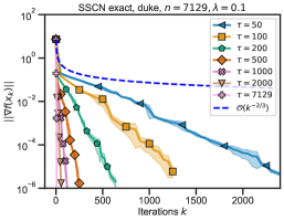
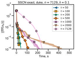
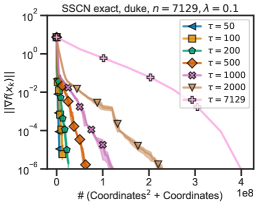
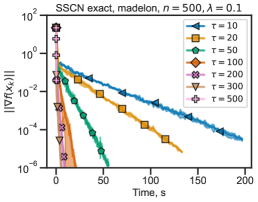
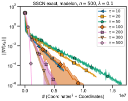
Figure 5: Convergence of different constant coordinate schedules measured w.r.t. iterations (first column), time (second column) and # (Coordinates² + Coordinates) evaluated (third column) averaged over three runs for logistic regression with non-convex regularization with $\lambda=0.1$ for two datasets. First row: duke, second row: madelon.

G.2 Constant vs. exponential schedule on more datasets

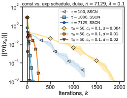
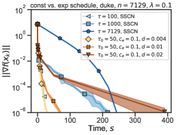
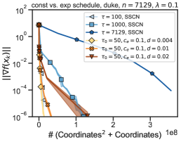
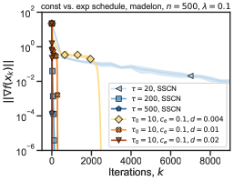
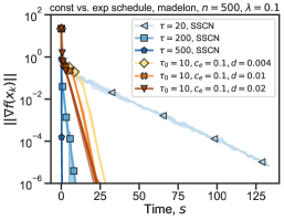
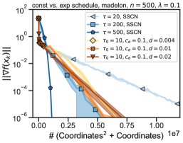
Figure 6: Comparison of constant vs. exponential schedules $\tau(S_{k})=\tau_{0}+c_{e}\exp(dk)$ for different parameters w.r.t. iterations (first column) and time (second column) and # (Coordinates² + Coordinates) evaluated (third column) averaged over three runs for logistic regression with non-convex regularization with $\lambda=0.1$ for the duke and madelon dataset.

G.3 CD vs. SSCN for more datasets

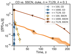
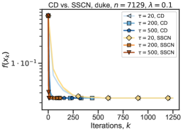
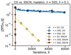
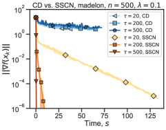
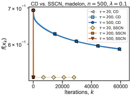
Figure 7: Comparison of CD and SSCN for different constant coordinate schedules measured w.r.t. iterations (first column) and time (second column) averaged over three runs for logistic regression with non-convex regularization with $\lambda=0.1$ for the duke and madelon dataset.

G.4 Convergence to an $\epsilon$-ball

We validate our prediction from Theorem 6 which guarantees the convergence to a ball whose radius is determined by $\epsilon_{1}$ and $\epsilon_{2}$, which in turn depends on the number of sampled coordinates $\tau(S)$. The larger $\tau(S)$, the smaller the radius of the ball, as stated in Lemma C.1 and Lemma C.2. In Figure 8 we can see that in the setting of binary logistic regression with non-convex regularizer $\lambda\cdot\sum_{i=1}^{n}{\bf x}_{i}^{2}/(1+{\bf x}_{i}^{2})$ indeed the gradient norm to which each constant coordinate schedule converges to decreases with increasing number of sampled coordinates.

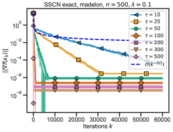
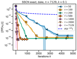
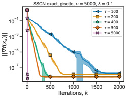
Figure 8: Convergence of different constant coordinate schedules measured w.r.t. iterations averaged over three runs for logistic regression with non-convex regularization with $\lambda=0.1$ for three different dataset. Plots correspond to the same setting as Figure 3 where the limits of the y-axis are chosen to be larger.

G.5 Adaptive schedule on gisette dataset

We also verify the proposed adaptive schedule from Eq. (17) on the gisette dataset, where we replaced the full gradient norm and Hessian Frobenius norm by estimates $\|\nabla f({\bf x}_{k})_{\text{est}}\|$ and $\|\nabla^{2}f({\bf x}_{k})_{\text{est}}\|_{2}$, which are estimated as exponential moving averages:

$$\|\nabla f({\bf x}_{k+1})_{\text{est}}\| =\alpha\|\nabla f({\bf x}_{k+1})_{[S]}\|+(1-\alpha)\|\nabla f({\bf x}_{k})_{\text{est}}\|$$ (86)

$$\|\nabla^{2}f({\bf x}_{k+1})_{\text{est}}\| =\alpha\|\nabla^{2}f({\bf x}_{k+1})_{[S]}\|+(1-\alpha)\|\nabla^{2}f({\bf x}_{k})_{\text{est}}\|,$$ (87)

where the weighting factor was chosen as $\alpha=0.2$. The proposed schedule $\tau(S_{k})_{\text{prop}}$ is further smoothed through an exponential moving average $\tau(S_{k+1})=\beta\cdot\tau(S_{k+1})_{\text{prop}}+(1-\beta)\tau(S_{k})$. As we can see the schedule is indeed close to an exponential schedule.

Figure 9: Evolution of $\|{\bf h}_{k}^{*}\|$ and $\tau(S_{k})$ for the gisette dataset for the adaptive coordinate schedule $\tau(S_{k})$.

References

• Agafonov et al. [2020] Artem Agafonov, Dmitry Kamzolov, Pavel Dvurechensky, Alexander Gasnikov, and Martin Takáč. Inexact tensor methods and their application to stochastic convex optimization. arXiv preprint arXiv:2012.15636, 2020.
• Byrd et al. [2011] Richard H Byrd, Gillian M Chin, Will Neveitt, and Jorge Nocedal. On the use of stochastic hessian information in optimization methods for machine learning. SIAM Journal on Optimization, 21(3):977–995, 2011.
• Carmon and Duchi [2019] Yair Carmon and John Duchi. Gradient descent finds the cubic-regularized nonconvex newton step. SIAM Journal on Optimization, 29(3):2146–2178, 2019.
• Cartis et al. [2011] Coralia Cartis, Nicholas IM Gould, and Philippe L Toint. Adaptive cubic regularisation methods for unconstrained optimization. part i: motivation, convergence and numerical results. Mathematical Programming, 127(2):245–295, 2011.
• Cartis et al. [2012] Coralia Cartis, Nicholas IM Gould, and Philippe L Toint. On the oracle complexity of first-order and derivative-free algorithms for smooth nonconvex minimization. SIAM Journal on Optimization, 22(1):66–86, 2012.
• Cartis et al. [2022] Coralia Cartis, Jaroslav Fowkes, and Zhen Shao. Randomised subspace methods for non-convex optimization, with applications to nonlinear least-squares. arXiv preprint arXiv:2211.09873, 2022.
• Chang and Lin [2011] Chih-Chung Chang and Chih-Jen Lin. LIBSVM: A library for support vector machines. ACM Transactions on Intelligent Systems and Technology, 2:27:1–27:27, 2011. Software available at http://www.csie.ntu.edu.tw/~cjlin/libsvm.
• Conn et al. [2000] Andrew R Conn, Nicholas IM Gould, and Philippe L Toint. Trust region methods. SIAM, 2000.
• Dennis and Moré [1977] John E Dennis, Jr and Jorge J Moré. Quasi-newton methods, motivation and theory. SIAM review, 19(1):46–89, 1977.
• Dereziński and Rebrova [2022] Michał Dereziński and Elizaveta Rebrova. Sharp analysis of sketch-and-project methods via a connection to randomized singular value decomposition. arXiv preprint arXiv:2208.09585, 2022.
• Doikov and Grapiglia [2023] Nikita Doikov and Geovani Nunes Grapiglia. First and zeroth-order implementations of the regularized Newton method with lazy approximated Hessians. arXiv preprint arXiv:2309.02412, 2023.
• Doikov and Nesterov [2020] Nikita Doikov and Yurii E Nesterov. Inexact tensor methods with dynamic accuracies. In ICML, pages 2577–2586, 2020.
• Doikov et al. [2023] Nikita Doikov, El Mahdi Chayti, and Martin Jaggi. Second-order optimization with lazy Hessians. In International Conference on Machine Learning. PMLR, 2023.
• Fuji et al. [2022] Terunari Fuji, Pierre-Louis Poirion, and Akiko Takeda. Randomized subspace regularized newton method for unconstrained non-convex optimization. arXiv preprint arXiv:2209.04170, 2022.
• Gower et al. [2019] Robert Gower, Dmitry Kovalev, Felix Lieder, and Peter Richtárik. Rsn: randomized subspace Newton. Advances in Neural Information Processing Systems, 32, 2019.
• Grapiglia et al. [2022] Geovani Nunes Grapiglia, Max LN Gonçalves, and GN Silva. A cubic regularization of Newton’s method with finite difference Hessian approximations. Numerical Algorithms, pages 1–24, 2022.
• Hanzely et al. [2020] Filip Hanzely, Nikita Doikov, Yurii Nesterov, and Peter Richtarik. Stochastic subspace cubic newton method. In International Conference on Machine Learning, pages 4027–4038. PMLR, 2020.
• Hanzely [2023] Slavomir Hanzely. Sketch-and-project meets newton method: Global o (k- 2) convergence with low-rank updates. 2023.
• Jorge and Stephen [2006] Nocedal Jorge and J Wright Stephen. Numerical optimization. Spinger, 2006.
• Kamzolov et al. [2023] Dmitry Kamzolov, Klea Ziu, Artem Agafonov, and Martin Takác. Cubic regularized quasi-Newton methods. arXiv preprint arXiv:2302.04987, 2023.
• Kohler and Lucchi [2017] Jonas Moritz Kohler and Aurelien Lucchi. Sub-sampled cubic regularization for non-convex optimization. In International Conference on Machine Learning, pages 1895–1904. PMLR, 2017.
• Kozak et al. [2019] David Kozak, Stephen Becker, Alireza Doostan, and Luis Tenorio. Stochastic subspace descent. arXiv preprint arXiv:1904.01145, 2019.
• Lacotte et al. [2021] Jonathan Lacotte, Yifei Wang, and Mert Pilanci. Adaptive newton sketch: Linear-time optimization with quadratic convergence and effective hessian dimensionality. In International Conference on Machine Learning, pages 5926–5936. PMLR, 2021.
• Lucchi and Kohler [2023] Aurelien Lucchi and Jonas Kohler. A sub-sampled tensor method for nonconvex optimization. IMA Journal of Numerical Analysis, 43(5):2856–2891, 2023.
• Nesterov [2012] Yurii Nesterov. Efficiency of coordinate descent methods on huge-scale optimization problems. SIAM Journal on Optimization, 22(2):341–362, 2012.
• Nesterov [2013] Yurii Nesterov. Introductory lectures on convex optimization: A basic course, volume 87. Springer Science & Business Media, 2013.
• Nesterov [2018] Yurii Nesterov. Lectures on convex optimization, volume 137. Springer, 2018.
• Nesterov and Polyak [2006] Yurii Nesterov and Boris T Polyak. Cubic regularization of newton method and its global performance. Mathematical Programming, 108(1):177–205, 2006.
• Nocedal and Wright [1999] Jorge Nocedal and Stephen J Wright. Numerical optimization. Springer, 1999.
• Patrascu and Necoara [2015] Andrei Patrascu and Ion Necoara. Efficient random coordinate descent algorithms for large-scale structured nonconvex optimization. Journal of Global Optimization, 61(1):19–46, 2015.
• Polyak [2007] Boris T Polyak. Newton’s method and its use in optimization. European Journal of Operational Research, 181(3):1086–1096, 2007.
• Richtárik and Takáč [2014] Peter Richtárik and Martin Takáč. Iteration complexity of randomized block-coordinate descent methods for minimizing a composite function. Mathematical Programming, 144(1-2):1–38, 2014.
• Scieur [2024] Damien Scieur. Adaptive quasi-Newton and Anderson acceleration framework with explicit global (accelerated) convergence rates. In International Conference on Artificial Intelligence and Statistics, pages 883–891. PMLR, 2024.
• Tripuraneni et al. [2018] Nilesh Tripuraneni, Mitchell Stern, Chi Jin, Jeffrey Regier, and Michael I Jordan. Stochastic cubic regularization for fast nonconvex optimization. Advances in neural information processing systems, 31, 2018.
• Ueda and Yamashita [2010] Kenji Ueda and Nobuo Yamashita. Convergence properties of the regularized newton method for the unconstrained nonconvex optimization. Applied Mathematics and Optimization, 62:27–46, 2010.
• Wang et al. [2018] Zhe Wang, Yi Zhou, Yingbin Liang, and Guanghui Lan. A note on inexact condition for cubic regularized newton’s method. arXiv preprint arXiv:1808.07384, 2018.
• Zhou et al. [2020] Dongruo Zhou, Pan Xu, and Quanquan Gu. Stochastic nested variance reduction for nonconvex optimization. The Journal of Machine Learning Research, 21(1):4130–4192, 2020.