Scale setting and hadronic properties in light quark sector with $(2+1)$-flavor Wilson fermions at the physical point

Abstract

We report scale setting and hadronic properties for our new lattice QCD gauge configuration set (HAL-conf-2023). We employ $(2+1)$-flavor nonperturbatively improved Wilson fermions with stout smearing and the Iwasaki gauge action on a $96^{4}$ lattice, and generate configurations of 8,000 trajectories at the physical point. We show the basic properties of the configurations such as the plaquette value, topological charge distribution and their auto-correlation times. The scale setting is performed by detailed analyses of the $\Omega$ baryon mass. We calculate the physical results of quark masses, decay constants of pseudoscalar mesons and single hadron spectra in light quark sector. The masses of the stable hadrons are found to agree with the experimental values within a sub-percent level.

I Introduction

Quantum Chromodynamics (QCD) governs the dynamics of quarks and gluons, and ultimately properties of hadrons and nuclei as well as nuclear astrophysical phenomena such as binary neutron star merges and nucleosynthesis. Currently, numerical lattice QCD simulation is the only available theoretical method which can solve QCD in a first-principle manner, and decades of theoretical progress together with the development of faster supercomputers enable us to make predictions (or postdictions) for basic hadronic quantities as well as quantities relevant to the search of physics beyond the Standard Model FlavourLatticeAveragingGroupFLAG:2021npn ; Aoyama:2020ynm ; Borsanyi:2020mff .

It remains, however, a great challenge to construct a bridge between QCD and nuclear physics by lattice QCD, since it is necessary to study multi-hadron systems on the lattice. For such studies, the so-called Signal(S)-to-Noise(N) problem appears generally, where the S/N ratio of the relevant correlation function becomes exponentially worse with lighter quark masses, a larger mass number and larger Euclidean time separation between source and sink operators Parisi:1983ae ; Lepage:1989hd . In addition, it is necessary to employ a larger lattice volume compared to that required for usual single hadron studies, in order to accommodate the longest interaction range (typically the range of the one-pion exchange) between two hadrons. It is clear that these problems are most pronounced with the physical (light) quark masses, while it is expected that physical point simulation is particularly important for nuclear physics due to the vital role of one- (and two-) pion exchanges.

The HAL QCD Collaboration significantly improved the situation recently, where we performed the first lattice QCD calculations for baryon-baryon interactions near the physical point Gongyo:2017fjb ; HALQCD:2018qyu ; HALQCD:2019wsz ; Lyu:2021qsh ; Aoki:2020bew . (See also Refs. Francis:2018qch ; Horz:2020zvv ; Amarasinghe:2021lqa ; Green:2021qol for recent studies for two-baryon systems at heavy quark masses based on Lüscher’s finite volume method.) Utilizing the (time-dependent) HAL QCD method Ishii:2006ec ; Ishii:2012ssm , which can significantly ameliorate the S/N problem Ishii:2012ssm ; Iritani:2018vfn , we performed comprehensive calculations of baryon-baryon interactions relevant to nuclear physics Aoki:2020bew as well as meson-meson Lyu:2023xro and meson-baryon interactions Lyu:2022imf at $(m_{\pi},m_{K})=(146,525)$ MeV on a large volume of $L^{4}=(8.1{\rm fm})^{4}$ with $N_{s}\equiv L/a=96$ and a lattice cutoff $a^{-1}=2.3$ GeV Ishikawa:2015rho . In these calculations, we employed the gauge configurations with $\sim$ 2,000 trajectories generated by the PACS Collaboration on the K computer, one of the fastest supercomputers in the world of that time. (We refer to this configuration set as “K-conf” hereafter.) Some of the highlights are the prediction of bound/virtual di-baryon states as $\Omega\Omega$ Gongyo:2017fjb , $\Omega_{ccc}\Omega_{ccc}$ Lyu:2021qsh , $N\Omega$ HALQCD:2018qyu , $N\Xi$ (remnant of H-dibaryon) HALQCD:2019wsz ; Kamiya:2021hdb as well as $\Xi$-hypernuclei Hiyama:2019kpw ; Hiyama:2022jqh and the exotic $T^{+}_{cc}$ state Lyu:2023xro .

Under these circumstances, the most important next step is to perform physical point simulations for nuclear physics. The results of di-baryons/hypernuclei/exotics mentioned above also indicate its importance. In fact, these states are found to be located near the unitary regime, and the importance of one- (or two-) pion exchange is explicitly observed in many of these states. Therefore, a tiny difference in quark masses could make a significant impact on the fate of these states. It is also implied that precision calculations with larger statistics are necessary.

In this paper, we report the generation of gauge configurations at the physical point by the HAL QCD Collaboration. We employ $(2+1)$-flavor nonperturbatively ${\cal O}(a)$-improved Wilson quark action with the stout smearing and the Iwasaki gauge action at $\beta=1.82$ on a $N_{s}^{4}=96^{4}$ box, as was the case for the K-conf. We, however, perform the simulation with the physical-point quark masses, which correspond to $(m_{\pi},m_{K})=(137.1(0.3)(^{+0.0}_{-0.2}),501.8(0.3)(^{+0.0}_{-0.7}))$ MeV. The lattice cutoff, $a^{-1}=2338.8(1.5)(^{+0.2}_{-3.0})$ MeV, is also determined in this paper using the mass of the $\Omega$ baryon. Physical values of quark masses, decay constants of pseudoscalar mesons and spectra of other hadrons are evaluated accordingly.

Numerical computations are performed on the supercomputer Fugaku, the new flagship supercomputer in Japan which succeeds the K computer. Fugaku was developed by the co-design of hardware and software, in which lattice QCD was one of the major targets of software applications Ishikawa:2021iqw . This enables efficient computations of the gauge configuration generation on Fugaku.

Before going to the main part, we have two remarks on our simulations. First, similar physical point generation was performed by the PACS Collaboration recently, with the same action and the same $(\beta,\kappa_{ud},\kappa_{s})$ but with two different volumes, $N_{s}^{4}=64^{4}$ and $128^{4}$, the latter of which is called “PACS10” configurations Ishikawa:2018jee ; PACS:2019ofv . With their determination of the cutoff, $a^{-1}=2316.2(4.4)$ MeV, the generation point for PACS10 configurations is found to be $(m_{\pi},m_{K})=(135.3(6)(3),497.2(2)(9))$ MeV. Unfortunately, the statistics are as small as $200$ trajectories and are insufficient to perform lattice QCD studies for nuclear physics. In this work, we generate $8,000$ trajectories in total with the benefit from their parameter tuning for the physical point. We also note that there is worldwide effort to generate configurations with various lattice QCD actions near or at the physical point PACS-CS:2008bkb ; PACS-CS:2009sof ; BMW:2008jgk ; BMW:2014pzb ; Ishikawa:2018jee ; PACS:2019ofv ; RBC:2012cbl ; RBC:2014ntl ; Bruno:2014jqa ; RQCD:2022xux ; Alexandrou:2018egz ; MILC:2012znn ; Bazavov:2017lyh .

Another remark is on the notion of “physical point” in our simulations. Since we perform $(2+1)$-flavor lattice QCD simulations without QED, the physical point can be defined only up to the uncertainties of isospin breaking effect (as well as much minor effect from dynamical heavy quarks). Since our primary target is to study nuclear physics from lattice QCD, in particular from the point of view of hadron interactions, we set our target values for the physical point by employing the isospin-averaged values of pseudoscalar meson masses, $(m_{\pi},m_{K})=(m_{\pi^{\rm ave}},m_{K^{\rm ave}})=(138,496)$ MeV.

This paper is organized as follows. In Sec. II, we give simulation details. In Sec. III, we show the basic properties of the generated ensemble by studying the plaquette value, the topological charge distribution, and their autocorrelation times. The analyses of the correlation functions of mesons and baryons are presented in Secs. IV and  V, respectively. In Sec. VII, we fix the scale of lattice spacing $a$ and show our results of hadron spectra, decay constants of pseudoscalar mesons and quark masses in physical units. Sec. VIII is devoted to summary and discussion.

II Simulation details

We generate $(2+1)$-flavor QCD configurations employing the Iwasaki gauge Iwasaki:1983iya and $\mathcal{O}(a)$-improved Wilson-clover quark actions. The lattice extent is $96^{4}$ and the lattice bare coupling constant $\beta\equiv 6/g^{2}=1.82$ following Refs. Ishikawa:2015rho ; Ishikawa:2018jee ; PACS:2019ofv .

The quark action is given by

$$S_{q=u,d,s} = \sum_{n}\bar{q}_{n}\left[q_{n}-\kappa_{q}c_{\text{SW}}\frac{i}{2}\sum_{\mu,\nu}\sigma_{\mu\nu}F_{\mu\nu}(n)q_{n}\right.$$

$$\left.-\kappa_{q}\sum_{\mu}\left\{(1-\gamma_{\mu})U_{n,\mu}q_{n+\hat{\mu}}+(1+\gamma_{\mu})U^{\dagger}_{n-\hat{\mu},\mu}q_{n-\hat{\mu}}\right\}\right],$$

where the gauge field is $6$ times smeared using the stout smearing parameter $\rho=0.1$. We utilize $c_{\text{SW}}=1.11$, which is nonperturbatively determined by the Schrödinger functional scheme in Ref. Taniguchi:2012gew . The hopping parameters for $u,d$ quarks and $s$ quark are set to $(\kappa_{ud},\kappa_{s})=(0.126117,0.124902)$, with which the hadron masses are reported to be almost the values at the physical point in Refs. Ishikawa:2018jee ; PACS:2019ofv . In our work, configurations are generated through 5 independent Markov chains ($5$-run series) by the hybrid Monte Carlo (HMC) algorithm, where different random number seeds and different initial configurations are used for each run. As initial configurations, we pick 5 configurations from the K-conf, which were generated with $(\kappa_{ud},\kappa_{s})=(0.126117,0.124790)$ corresponding to slightly heavier quark masses than the physical point Ishikawa:2015rho . After discarding more than $300$ trajectories for the thermalization process in each run, we generate $1,600$ trajectories in each run, thus, $8,000$ trajectories in total. We save the configurations every $5$ trajectories and use them for the measurement of physical quantities, e.g., topological charge and hadron correlation functions.

Let us explain how to implement the quark action in HMC in detail. We symbolically rewrite the Wilson-clover operator as

$$D=1+T+M,$$ (2)

where $T$ and $M$ denote the clover and the hopping terms, respectively. As for the $u,d$ quarks with degenerated masses, we divide the corresponding quark action, $|\det D|^{2}$, into several factors as follows. First of all, factorization of the clover term as $D=(1+T)(1+(1+T)^{-1}D)\equiv(1+T)\tilde{D}$ gives

$$|\det D|^{2}=|\det(1+T)|^{2}|\det\tilde{D}|^{2}.$$ (3)

Since the term $(1+T)$ consists of the local quantities, it is easy to simulate the first factor in the determinant. On the other hand, the calculation of the second factor is expensive, so that we utilize the domain-decomposed HMC (DDHMC) algorithm Luscher:2003vf , the Hasenbusch mass preconditioning Hasenbusch:2001ne ; Hasenbusch:2002ai , and the even-odd preconditioning.

The Dirac operator $\tilde{D}$ is decomposed by the even ($E$) and odd ($O$) domains,

$$\tilde{D}=\begin{pmatrix}\tilde{D}_{EE}&\tilde{D}_{EO}\\ \tilde{D}_{OE}&\tilde{D}_{OO}\\ \end{pmatrix}.$$ (4)

Utilizing the Schur decomposition, we rewrite $|\det\tilde{D}|^{2}$ as

$$\left|\det\tilde{D}\right|^{2} =\left|\det\tilde{D}_{EE}\right|^{2}\left|\det\tilde{D}_{OO}\right|^{2}\left|\det[1-(\tilde{D}_{EE}^{-1}\tilde{D}_{EO}\tilde{D}_{OO}^{-1}\tilde{D}_{OE})]\right|^{2}.$$

Introducing the even-odd site decomposition in each domain and the spin projection that connects even-odd sites, each determinant can be written by

$$\det\tilde{D}_{EE}=\det[(\hat{D}_{EE})_{ee}],$$

$$\det\tilde{D}_{OO}=\det[(\hat{D}_{OO})_{ee}],$$

$$\det[1-(\tilde{D}_{EE}^{-1}\tilde{D}_{EO}\tilde{D}_{OO}^{-1}\tilde{D}_{OE})]=\det[\hat{D}_{EE}^{\mathrm{spin}}],$$ (5)

where we refer to Ref. PACS-CS:2008bkb for the explicit form of the spin projection.

Now, we can implement the $u,d$ quark action using three pseudo fermions ($\phi_{O_{e}},\phi_{Ee}$ and $\chi_{E}$),

$$S_{ud} = -\log\left(|\det D|^{2}\right)$$ (6)

$$\rightarrow -2\mathrm{Tr}\log(1+T)+\sum_{X=E,O}\left|((\hat{D}_{XX})_{ee})^{-1}\phi_{Xe}\right|^{2}+\left|(\hat{D}_{EE}^{\mathrm{spin}})^{-1}\chi_{E}\right|^{2}$$

$$\coloneqq S_{ud,\mathrm{clv.}}[U;\kappa_{ud}]+\sum_{X=E,O}S_{ud,\mathrm{UV}}[U,\phi_{Xe};\kappa_{ud}]+S_{ud,\mathrm{IR}}[U,\chi_{E};\kappa_{ud}].$$

The calculations of the first and second terms can be performed within each domain, while the third term describes the long-range modes and the simulation of this term requires data transfer between different domains. Therefore, we introduce the two-fold Hasenbusch preconditioning to speed up the simulation. By introducing $\kappa_{1}=\rho_{1}\kappa_{ud}$ and $\kappa_{2}=\rho_{2}\kappa_{1}$ ($\rho_{1},\rho_{2}<1$) with two additional pseudo fermions, $\zeta_{E}^{1},\zeta_{E}^{2}$, the third term is decomposed into three parts,

$$\left|(\hat{D}_{EE}^{\mathrm{spin}}(\kappa_{ud}))^{-1}\chi_{E}\right|^{2} \rightarrow \left|\frac{\hat{D}_{EE}^{\mathrm{spin}}(\kappa_{1})}{\hat{D}_{EE}^{\mathrm{spin}}(\kappa_{ud})}\zeta_{E}^{1}\right|^{2}+\left|\frac{\hat{D}_{EE}^{\mathrm{spin}}(\kappa_{2})}{\hat{D}_{EE}^{\mathrm{spin}}(\kappa_{1})}\zeta_{E}^{2}\right|^{2}+\left|(\hat{D}_{EE}^{\mathrm{spin}}(\kappa_{2}))^{-1}\chi_{E}\right|^{2}$$ (7)

$$\coloneqq S_{{ud},\mathrm{IR1}}+S_{{ud},\mathrm{IR2}}+S_{{ud},\mathrm{IR3}}$$

In this work, we tune the values of $\rho_{1}$ and $\rho_{2}$ as $\rho_{1}=0.99975$ and $\rho_{2}=0.99600$, respectively.

The strange quark part is implemented by the rational hybrid Monte Carlo (RHMC) algorithm Clark:2006fx . The clover term is factored out as in the case of the $u,d$ quarks, $D=(1+T)\tilde{D}$, and the weight factor associated with the second term is evaluated with the rational approximation. For the calculations of the force, the range of the approximation for the rational functions of $x=\tilde{D}^{\dagger}\tilde{D}$ is taken as $[x_{\rm min},x_{\rm max}]=[0.000200000001,2]$ with the order of $N_{\mathrm{\mathrm{RHMC,F}}}=10$ expansion, which ensures $10^{-7}$ accuracy for $1/\sqrt{x}$. Note that these parameters for the rational approximation of the force are fixed during the steps of molecular dynamics (MD) in order to fix the equation of motion of the MD. We also checked that our simulation is actually within the range of $[x_{\rm min},x_{\rm max}]$. On the other hand, in the calculation of the strange quark Hamiltonian for the Metropolis test, the approximation range is chosen from min and max eigenvalues of the $\tilde{D}^{\dagger}\tilde{D}$ operator (with an additional margin factor of $1.01$ for both min and max), and the order of the approximation, $N_{\mathrm{RHMC,H}}$, is tuned to keep $10^{-14}$ accuracy (typically $N_{\mathrm{RHMC,H}}=20$ is chosen.).

Corresponding to each term in the action, we have the following force terms in the MD steps in the HMC algorithm: the gauge force $F_{g}$ from the gauge action, the clover force $F_{ud,\mathrm{clv.}}$, the UV force $F_{ud,\mathrm{UV}}$ and the three IR parts $F_{ud,\mathrm{IR1}}$, $F_{ud,\mathrm{IR2}}$, $F_{ud,\mathrm{IR3}}$ from the $u,d$ quark actions, and the clover force $F_{s,\mathrm{clv.}}$ and the RHMC force $F_{s,\mathrm{RHMC}}$ from the $s$ quark action. In the MD steps, we adopt the multiple time scale integration scheme Sexton:1992nu with a depth of 5, where the hierarchy of forces is taken as follows: $F_{5}=F_{g}$, $F_{4}=F_{ud,\mathrm{UV}}$, $F_{3}=F_{ud,\mathrm{IR3}}+F_{s,\mathrm{RHMC}}+F_{ud,\mathrm{clv.}}+F_{s,\mathrm{clv.}}$ $F_{2}=F_{ud,\mathrm{IR2}}$, $F_{1}=F_{ud,\mathrm{IR1}}$,

We employ the leapfrog algorithm for the MD evolution, as in the case of Refs. PACS-CS:2008bkb ; PACS-CS:2009sof ; Ishikawa:2015rho ; Ishikawa:2018jee ; PACS:2019ofv , since we find that the Omelyan algorithm is less stable. In the solver for the pseudo fermions, we impose the stopping condition of $|r_{\rm crit}|<10^{-14}$ for the evaluations of both the forces and the Hamiltonian so that the reversibility in the MD evolution and the accuracy of the Metropolis test are assured PACS-CS:2008bkb ; PACS-CS:2009sof ; Ishikawa:2015rho . For the IR part of the $u,d$ quarks, we employ the mixed precision nested BiCGStab solver with the Schwarz Alternating Procedure (SAP) and point Jacobi iteration preconditioners PACS-CS:2008bkb ; Ishikawa:2021iqw . The code optimization for Fugaku developed in the QWS library Ishikawa:2021iqw is utilized in the quark solver. Within one MD trajectory ($\delta\tau_{\mathrm{MD}}=1.0$), the time step of the MD evolution is implemented using a set of integers ($N_{5},N_{4},N_{3},N_{2},N_{1}$) for each force calculation: $\delta\tau_{5}=\delta\tau_{\mathrm{MD}}/(N_{5}N_{4}N_{3}N_{2}N_{1})$, $\delta\tau_{4}=\delta\tau_{\mathrm{MD}}/(N_{4}N_{3}N_{2}N_{1})$, $\delta\tau_{3}=\delta\tau_{\mathrm{MD}}/(N_{3}N_{2}N_{1})$, $\delta\tau_{2}=\delta\tau_{\mathrm{MD}}/(N_{2}N_{1})$, and $\delta\tau_{1}=\delta\tau_{\mathrm{MD}}/N_{1}$. We take ($N_{5},N_{4},N_{3},N_{2},N_{1}$) $=$ ($8,2,2,2,22$). Figure 1 depicts the history of the force average in each MD trajectory. Figure 2 represents the difference of Hamiltonian, $dH$, for each MD trajectory. While there are several spikes in total $8,000$ trajectories, the simulation is basically stable during the MD evolution. It results in the $87$% acceptance rate.

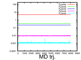
Figure 1: History of the force average in the MD evolution.

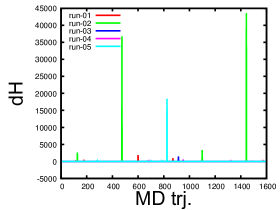
Figure 2: History of difference of Hamiltonian, $dH$, in the MD evolution for each run.

In Fig. 3, we show the plaquette values calculated by the jackknife method with different bin sizes. As a central value, we take the bin size $=100$ trajectories and obtain $\langle\mathrm{plaquette}\rangle=0.5039576(3)$. Our result is $1\sigma$ consistent with the data by the PACS Collaboration on $64^{4}$ and $128^{4}$ lattices with the same $\beta$ and $\kappa_{ud},\kappa_{s}$ Ishikawa:2018jee ; PACS:2019ofv , but the statistical errors of our data are much smaller thanks to our higher statistics. We summarize basic data for the configuration generation in Table 1. All statistical errors are estimated by the jackknife method with the bin size of $100$ trajectories.

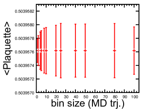
Figure 3: Bin-size dependence in the jackknife analysis for the plaquette average.

$\langle$ plaquette $\rangle$	$\langle e^{-dH}\rangle$	acc. rate	$\langle F_{5}\rangle$	$\langle F_{4}\rangle$	$\langle F_{3}\rangle$	$\langle F_{2}\rangle$	$\langle F_{1}\rangle$
0.5039576(3)	0.991(4)	0.872	4.689783(1)	0.340328(1)	0.217155(2)	0.009101(5)	0.000110(1)

Table 1: Detail data of configuration generation

III Ensemble properties: auto correlation

In this section, we show the ensemble properties of generated configurations by investigating several local observables such as the energy density as a function of the gradient flow time and the topological charge distribution. Furthermore, we study the integrated auto-correlation time of these quantities. As will be shown below, the resulting integrated auto-correlation times are found to be reasonably short (less than $10$ trajectories) even for the topological charges. This indicates that an independent configuration set has been generated.

To measure the topological charge distribution, we adopt the definition of the topological charge through the gradient flow Luscher:2010iy . The gradient flow is defined by the following equations

$$\partial_{t}V_{t}(x,\mu) = -g_{0}^{2}\{\partial_{x,\mu}S(V_{t})\}V_{t}(x,\mu),$$ (8)

$$V_{t}(x,\mu)|_{t=0} = U(x,\mu),$$ (9)

where $x=(\vec{x},\tau)$ is the space-time lattice point and $t$ is the flow-time, $V_{t}(x,\mu)$ denotes the smeared link variables over a radius $r=\sqrt{8t}$ at the flow-time $t$, and $U(x,\mu)$ is the generated link variable in Monte Carlo calculations. Here, $S$ represents the flow gauge action, which we can choose independently from the gauge action in the configuration generation process. In our work, we utilize the standard plaquette gauge action as a flow gauge action to solve the differential equation Eq. (8). We use the third-order Runge-Kutta algorithm with a step size $\varepsilon=0.01$.

The gluonic definition of the topological charge density can be given by

$$q(x,t)=-\frac{1}{32\pi^{2}}\epsilon_{\mu\nu\rho\sigma}\mathrm{tr}\{G_{\mu\nu}(x,t)G_{\rho\sigma}(x,t)\},$$ (10)

with a clover-type definition of the field strength $G_{\mu\nu}(x,t)$, which is constructed by the smeared link variables $V_{t}$. The topological charge can be directly calculated by the topological charge density in Eq. (10),

$$Q(t)=a^{4}\sum_{x}q(x,t).$$ (11)

The value of $Q(t)$ roughly plateaus in a long $t$ region, but small fluctuations exist. Therefore, we introduce a reference scale $t_{0}$ and identify the value of $Q(t=t_{0})$ as a convergent value of $Q$ for each configuration Bruno:2014ova .

The reference scale $t_{0}$ is originally introduced in Ref. Luscher:2010iy , which is given by

$$t^{2}\langle E(t)\rangle|_{t=t_{0}}=0.3,$$ (12)

where $E(t)$ denotes the energy density

$$E(t)=-\frac{1}{2V}\sum_{x}\mathrm{tr}\{G_{\mu\nu}(x,t)G_{\mu\nu}(x,t)\}.$$ (13)

Here, we utilize a clover-type definition for $G_{\mu\nu}(x,t)$ again.

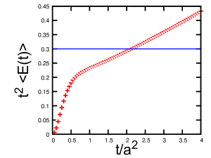
Figure 4: Data of $t^{2}\langle E(t)\rangle$ as a function of the gradient flow time, $t/a^{2}$.

Figure 4 depicts the dimensionless energy density $t^{2}\langle E(t)\rangle$ as a function of the flow-time $t$. We obtain

$$t_{0}/a^{2}=2.1047(4)$$ (14)

as an averaged value of $t_{0}$ in lattice unit results. We also calculate a similar reference scale,

$$w_{0}/a=2.0126(4),$$ (15)

which is defined by BMW:2012hcm

$$\left.t\frac{d}{dt}\left\{t^{2}\langle E(t)\rangle\right\}\right|_{t=w_{0}^{2}}=0.3.$$ (16)

Figure 5 represents the histogram of $Q(t_{0})$ for total $1,600$ generated configurations.

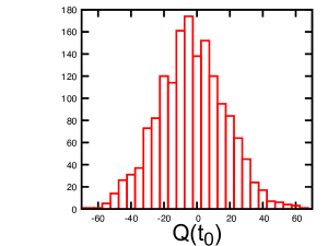
Figure 5: Histogram of the topological charge $Q(t)$ at $t=t_{0}$.

It shows almost a Gaussian distribution as expected. Table 2 is the summary of the averaged values of $Q(t_{0})$ and $Q(t_{0})^{2}$, and the susceptibility $\chi_{Q}=\langle(Q-\langle Q\rangle)^{2}/V$. As expected, $\langle Q\rangle$ is consistent with zero within $1.1\sigma$ uncertainty.

$\langle Q\rangle$	$\langle Q^{2}\rangle$	$\chi_{Q}$
$-0.6644(6167)\quad$	$\quad 416.8(16.1)\quad$	$\quad 4.90(19)\times 10^{-6}$

Table 2: Averages and statistical errors of $Q$, $Q^{2}$ and the topological susceptibility $\chi_{Q}$.

Now, let us estimate the auto-correlation times of local observables. We follow the papers RBC:2012cbl ; RBC:2014ntl to define the integrated auto-correlation time and its error estimation. The integrated auto-correlation time $\tau_{\mathrm{i}nt.}$ for the observable $A$ as a function of the cutoff in MD time separation ($\Delta_{\mathrm{cut}}$) is given by

$$\tau_{\mathrm{int.}}(\Delta_{\mathrm{cut}})=\frac{1}{2}+\sum_{\Delta=1}^{\Delta_{{\mathrm{cut}}}}C(\Delta),$$ (17)

where

$$C(\Delta)=\left\langle\frac{(A_{i}-\bar{A})(A_{i+\Delta}-\bar{A})}{\sigma^{2}}\right\rangle_{i}$$ (18)

with the index $i$ denoting the MD time. Here, $\bar{A}$ and $\sigma$ represent the mean and variance of $A_{i}$. We first calculate them using the jackknife method with a sufficiently large bin size. By referring to Fig. 3, we take $20$ MD trajectories in our analyses. Next, we bin the data inside the brackets in Eq. (18) for a fixed $\Delta$. Here, the bin size can be taken independently of the first bin size in the jackknife method. We increase it until the statistical error of $\tau_{\mathrm{int.}}$ saturates. The statistical error of $\tau_{\mathrm{int.}}$ is estimated by the bootstrap method by resampling the binned data inside the brackets in Eq. (18).

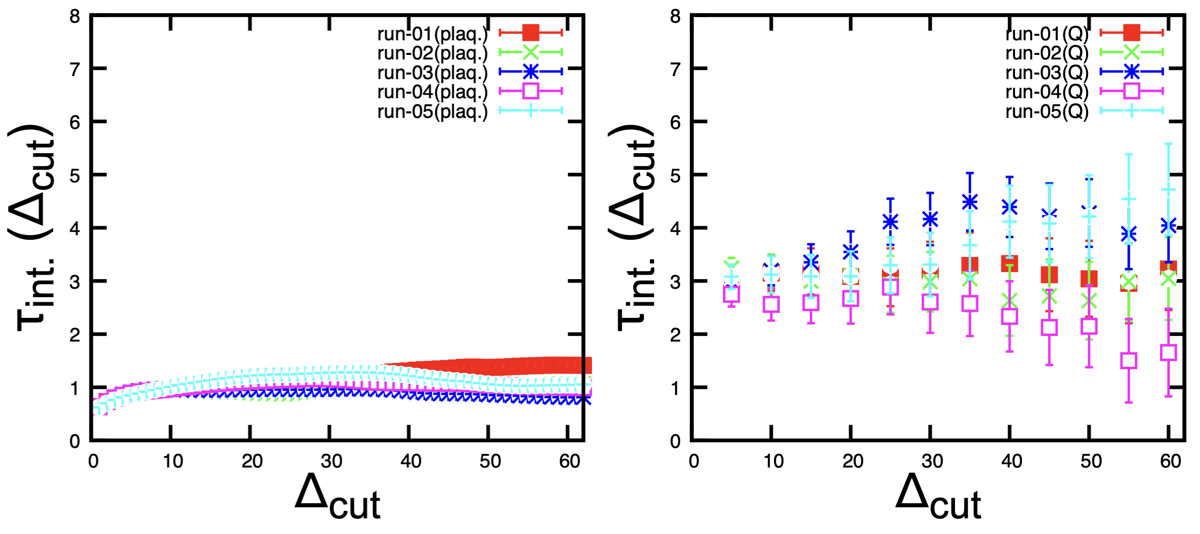
Figure 6: Integrated auto-correlation time $\tau_{\mathrm{int.}}$ for the plaquette (left) and topological charge ($Q(t_{0})$) (right) as a function of $\Delta_{\mathrm{cut}}$ for each run.

Figure 6 displays the integrated auto-correlation times for the plaquette and topological charge ($Q(t_{0})$) in the left and right panels, respectively. Here, we analyze our data for each run series independently. We observe that the obtained integrated auto-correlation times saturate in short trajectory regions, namely at most $2$ MD trajectories for the plaquette and $6$ MD trajectories for the topological charge.

In order to further confirm such a short auto-correlation time, we study the history of $Q$ in the MD evolution. As shown in Fig. 7, we find that the value of $Q$ indeed changes significantly even for $1$ configuration separation corresponding to 5 MD trajectory separation.

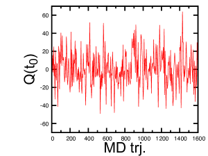
Figure 7: History of the topological charge $Q(t_{0})$ in the MD evolution for the run-01 configurations.

There are two possible reasons for this short auto-correlation time. One is the use of the Wilson fermions, where the near-zero mode is absent even in a small quark mass regime. The other is that the lattice spacing in our simulation, which will be determined as $a\approx 0.08$fm later in this paper, is relatively coarse compared to the spacing where the topological freezing starts to appear. Consequently, the short auto-correlation time suggests that our set of $1,600$ configurations is well spread in the configuration space and serves as good ensembles for lattice QCD measurements of physical quantities.

IV Stable Mesons

IV.1 Calculation strategy

We study the meson spectra, the decay constants and the PCAC masses for $u,d$ and $s$ quarks from the two-point correlation functions.

The local operators for flavor off-diagonal pseudo-scalar (PS) and axial-vector current with zero-momentum projection are defined by

$$P(\tau) = \sum_{\vec{x}}\bar{q}_{f}(\vec{x},\tau)\gamma_{5}q_{g}(\vec{x},\tau),$$ (19)

$$A_{\mu}(\tau) = \sum_{\vec{x}}\bar{q}_{f}(\vec{x},\tau)\gamma_{\mu}\gamma_{5}q_{g}(\vec{x},\tau).$$ (20)

Here, the indices $f,g$ with $f\neq g$ label the flavor of the valence quarks ($f,g=u,d,s$). In terms of the operator improvement of the axial-vector current, $A_{\mu}(\tau)\rightarrow A_{\mu}(\tau)+ac_{A}\partial_{\mu}P(\tau)$, we employ the tree-level value, $c_{A}=0$, since it is expected to be a good approximation in our lattice setup thanks to the link smearing for the fermion BMW:2010skj ; BMW:2013fzj , and the explicit non-perturbative calculation found that $c_{A}$ is indeed consistent with zero within the statistical error Taniguchi:2012gew .

To measure the correlation function between the currents, we employ the wall source method without gauge fixing Kuramashi:1993ka . Quark propagators are solved with the periodic boundary condition for all directions, where the stopping conditions are taken as $|r_{\rm crit}|<10^{-6}$ for $u,d$ quarks and $|r_{\rm crit}|<10^{-12}$ for $s$ quark. We have checked that these stopping conditions are sufficiently precise in our study. To suppress statistical fluctuations, we take the average between forward and backward propagation, and we also measure the correlation function in each of the four directions for one configuration using the fact that our lattice has hypercubic symmetry. Thus, the total number of measurements for the observables in this section is $1600\times 4\times 2=12,800$. The statistical errors in this section are estimated by the jackknife method.

To obtain the PS meson masses ($m_{\mathrm{PS}}$), the PCAC quark masses and the PS meson decay constants, we utilize the PS-PS correlators and PS-A₄ correlators as follows. The PS-PS correlators at $\tau/a,(T-\tau)/a\rightarrow\infty$ are expressed by

$$\langle P(\tau)P^{\dagger}(0)\rangle \simeq N_{s}^{3}C_{PP}W(m_{\mathrm{PS}}T)\times\left[\exp(-m_{\mathrm{PS}}\tau)+\exp(-m_{\mathrm{PS}}(T-\tau))\right],$$ (21)

where $W(m_{\mathrm{PS}}T)$ with $T/a=96$ counts the contribution from wrapping propagation of the PS meson around the lattice in the temporal direction. This is given as the sum of zero to infinite windings,

$$W(m_{\mathrm{PS}}T) = 1+\exp(-m_{\mathrm{PS}}T)+\exp(-2m_{\mathrm{PS}}T)+\cdots,$$ (22)

$$= \frac{1}{1-\exp(-m_{\mathrm{PS}}T)}.$$

Similarly, the PS-A₄ correlators at $\tau/a,(T-\tau)/a\rightarrow\infty$ have the following form,

$$\langle A_{4}(\tau)P^{\dagger}(0)\rangle \simeq N_{s}^{3}C_{AP}W(m_{\mathrm{PS}}T)\times\left[\exp(-m_{\mathrm{PS}}\tau)-\exp(-m_{\mathrm{PS}}(T-\tau))\right].$$ (23)

We define the PCAC bare quark masses through axial Ward identity (AWI) as

$$m_{f}^{\rm AWI}+m_{g}^{\rm AWI}=\frac{\langle 0|\partial_{4}A_{4}|PS\rangle}{\langle 0|P|PS\rangle}.$$ (24)

They can be evaluated with

$$m_{f}^{\rm AWI}+m_{g}^{\rm AWI}=m_{\mathrm{PS}}\left|\frac{C_{AP}}{C_{PP}}\right|,$$ (25)

using the parameters given in Eqs. (21) and (23).

As for the decay constants of the PS mesons, we utilize the following expression for the bare values,

$$f_{\mathrm{PS},fg}^{\rm bare}=\sqrt{2\kappa_{f}}\sqrt{2\kappa_{g}}\frac{\sqrt{2}|C_{AP}|}{\sqrt{m_{\mathrm{PS}}|C_{PP}|}}.\quad$$ (26)

In our analysis, we first study the effective masses of the PS mesons, defined locally in time using two data points, $\tau$ and $\tau+a$ of Eq. (21) (or Eq. (23)), and examine the ground state saturation. The effective PCAC quark masses are studied by using Eq. (24), where the derivative of $A_{4}$ is estimated by the forth-order symmetric difference.

To obtain our main results, we perform simultaneous fit of Eqs. (21) and (23) to determine best-fit values of $m_{\mathrm{PS}},C_{PP}$ and $C_{AP}$, from which the PS meson masses and the bare values of the PCAC masses and decay constants are obtained.

In order to obtain the physical values of the quark masses and decay constants, we consider the ${\cal O}(ma)$ improvement and the renormalization factors. The expressions for the ${\cal O}(ma)$ improvement are given by Bhattacharya:2005rb

$$m_{fg}^{\rm imp.}=\left[\frac{1+ab_{A}m_{fg}+a\bar{b}_{A}{\rm Tr}M}{1+ab_{P}m_{fg}+a\bar{b}_{P}{\rm Tr}M}\right]m_{fg}^{\rm AWI},$$ (27)

$$f_{\mathrm{PS},fg}^{\rm imp.}=\left[1+ab_{A}m_{fg}+a\bar{b}_{A}{\rm Tr}M\right]f_{\mathrm{PS},fg}^{\rm bare},$$ (28)

where $m_{fg}\equiv(m_{f}+m_{g})/2$ and $M\equiv{\rm diag}(m_{u},m_{d},m_{s})$ represent the bare quark masses, and $b_{A},\bar{b}_{A}$ and $b_{P},\bar{b}_{P}$ are improvement coefficients for axial-vector and pseudo-scalar currents, respectively. Note that these formulae are valid for flavor non-singlet operators  .

As regards the bare quark masses in the improvement terms, $m_{f}$, one may employ those associated with axial Ward identity (AWI), $m_{f}^{\rm AWI}$, or with vector Ward identity (VWI), $\displaystyle m_{f}^{\rm VWI}\equiv\frac{1}{a}\left(\frac{1}{2\kappa_{f}}-\frac{1}{2\kappa_{c}}\right)$ with $\kappa_{c}$ being the critical hopping parameter, as far as the improvement coefficients are defined consistently. The relation between the two definitions is given as Bhattacharya:2005rb

$$m_{fg}^{\rm AWI} = \frac{Z_{P}Z_{m}}{Z_{A}}\left[m_{fg}^{\rm VWI}+(r_{m}-1)\frac{{\rm Tr}M^{\rm VWI}}{N_{f}}\right]+{\cal O}(a),$$ (29)

$${\rm Tr}M^{\rm AWI} = \frac{Z_{P}Z_{m}}{Z_{A}}r_{m}{\rm Tr}M^{\rm VWI}+{\cal O}(a),$$ (30)

where $Z_{A},Z_{P}$ and $Z_{m}$ denote the renormalization factor in flavor non-singlet sector for the axial-vector current, for the pseudo-scalar current, and for the VWI quark mass, respectively, and $r_{m}$ is the ratio of renormalization factors between flavor singlet and non-singlet sectors for the VWI quark mass. In order to evaluate the ${\cal O}(ma)$ improvement terms in Eqs. (27) and (28), we employ the tree-level values, $Z_{A}=Z_{P}=Z_{m}=r_{m}=1$ and $b_{A}=b_{p}=1,\bar{b}_{A}=\bar{b}_{P}=0$, and with $m_{f}$ substituted by $m_{f}^{\rm AWI}$. In perturbation theory, the correction to the tree-level value is ${\cal O}(g_{0}^{4})$ for $r_{m},\bar{b}_{A},\bar{b}_{P}$ and ${\cal O}(g_{0}^{2})$ for others. In our lattice setup, we expect such corrections are well suppressed thanks to the stout smearing. In fact, in the case of $Z_{A}$ and $Z_{P}$, the values determined non-perturbatively are found to agree with the tree-level values within a few percent errors Ishikawa:2015fzw . Considering also that the magnitude of the improvement term is small, we neglect the uncertainties associated with the tree-level evaluation of the ${\cal O}(ma)$ improvement.

Finally, we obtain the physical values for the quark masses and decay constants by

$$m_{fg}^{\rm\overline{MS}} = \frac{Z_{A}}{Z_{P}}m_{fg}^{\rm imp.},$$ (31)

$$f_{\mathrm{PS},fg} = Z_{A}f_{\mathrm{PS},fg}^{\rm imp.}.$$ (32)

In our calculation, we take $(Z_{A}/Z_{P})^{\rm\overline{MS}}=Z_{m}^{\rm\overline{MS}\leftarrow SF}\cdot(Z_{A}/Z_{P})^{\rm SF}=0.9950(142)$ at $\mu=$ 2 GeV and $Z_{A}=0.9650(117)$ where $Z_{A},Z_{P}$ are determined nonperturbatively in the Schrödinger functional (SF) scheme and $Z_{m}^{\rm\overline{MS}\leftarrow SF}$ is the mass matching factor between SF and ${\rm\overline{MS}}$ schemes Ishikawa:2015fzw . The uncertainties of the renormalization factors are included in the systematic errors of our results.

In terms of the quark masses, we remark that there exists another formula called the ratio-difference method BMW:2010skj . While we do not use this method in this work, we give a quick summary for this method in Appendix A, where we argue that it is necessary to modify the formula known in the literature in order to respect that Eq. (27) is valid only for flavor non-singlet sectors.

IV.2 Numerical results: PS meson spectra and PCAC quark masses

Here, we present our numerical results. In Fig. 8, we show the effective masses of the PS mesons using the PS-PS correlators in the light-light quark sector ($q_{f},q_{g}=q_{u,d}$ in Eq. (21)) for pion and in the light-heavy quark sector ($q_{f}=q_{u,d}$ and $q_{g}=q_{s}$) for kaon. We observe clear plateaux for both PS mesons. The results from the PS-A₄ correlators show similar behavior.

The PS meson masses are obtained by the simultaneous fit of the PS-PS and PS-A₄ correlators of Eqs. (21) and (23), where the fit range is taken to be $17\leq\tau/a\leq 41$ for the light-light quark sector and $25\leq\tau/a\leq 39$ for the light-heavy quark sector. The corresponding fit results as well as the statistical errors are shown by the black lines with gray bands in Fig. 8. We also study the systematic errors by investigating the fit range dependence.

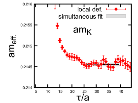
Figure 8: Effective masses for pion (left) and kaon (right) obtained from the PS-PS correlators. The black lines with gray bands depict the results with statistical errors obtained by the simultaneous fit of the PS-PS and PS-A₄ correlators.

In Fig. 9, we show the effective PCAC bare quark masses for $u,d$ and $s$ quarks. The $u,d$ quark mass is obtained from correlators in the light-light quark sector, while the $s$ quark mass is obtained from the combination of correlators in the light-light and light-heavy quark sectors. Clear plateaux are observed in both quark masses. Shown together by the black lines with gray bands in Fig. 9 are the results with statistical errors from the simultaneous fit of the PS-PS and PS-A₄ correlators combined with Eq. (25).

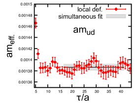
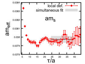
Figure 9: Effective masses for the PCAC bare quark masses for $u,d$ (left) and $s$ (right) quarks obtained from the combinations of the PS-PS and PS-A₄ correlators in light-light and light-heavy quark sectors. The black lines with gray bands depict the results with statistical errors obtained by the simultaneous fit of the PS-PS and PS-A₄ correlators.

The summary of the results for the PS meson masses and PCAC bare quark masses are tabulated in Table 3. Our result of $m_{s}/m_{ud}=27.39(11)(^{+1}_{-0})$ is found to be consistent with the FLAG average value for $(2+1)$-flavor QCD, $m_{s}/m_{ud}=27.42(12)$ FlavourLatticeAveragingGroupFLAG:2021npn .

$am_{ud}$	$am_{s}$	$m_{s}/m_{ud}$	$am_{\pi}$	$am_{K}$
$0.001386(6)(^{+1}_{-0})\quad$	$\quad 0.037974(40)(^{+2}_{-2})\quad$	$\quad 27.39(11)(^{+1}_{-0})\quad$	$\quad 0.058606(152)(^{+10}_{-13})\quad$	$\quad 0.214552(43)(^{+1}_{-4})$

Table 3: The results for PCAC (AWI) bare quark masses and PS meson masses in lattice units. The errors in the first parentheses are statistical ones and those in the second parentheses are systematic ones originating from the fit-range uncertainty of the simultaneous fit.

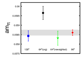
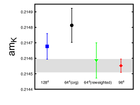
Figure 10: Comparison of our results and PACS results Ishikawa:2018jee for pion mass (left) and kaon mass (right) in lattice units, where the error bars are statistical. Our results obtained on a $96^{4}$ lattice are shown in red diamonds with gray bands depicting our statistical errors. The PACS results on $128^{4}$, $64^{4}$ (org) and $64^{4}$ (reweighted) lattices are shown by blue squares, black circles and green triangles, respectively, where $64^{4}$ (org) and $64^{4}$ (reweighted) denote results at the simulation point and those at the reweighted point for $(\kappa_{ud},\kappa_{s})$ parameters.

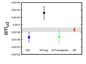
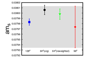
Figure 11: Same as Fig. 10, but for PCAC (AWI) bare quark masses for $u,d$ (left) and $s$ (right) quarks in lattice units.

We also compare our numerical results on a $96^{4}$ lattice with those given by the PACS Collaboration on $128^{4}$ and $64^{4}$ lattices Ishikawa:2018jee ; PACS:2019ofv , since we take the same simulation parameters, ($\beta,\kappa_{ud},\kappa_{s}$), with theirs. We note that, in the case of the PACS results on a $64^{4}$ lattice, the results at the simulation point (referred to $64^{4}$ (org)) correspond to those at slightly different physical quark masses due to the finite volume effect on $\kappa_{c}$, so the results at the reweighted $(\kappa_{ud},\kappa_{s})$ parameters (referred to $64^{4}$ (reweighted)) are the relevant ones to be compared with Ishikawa:2018jee .

Figure 10 shows the comparison for the pion and kaon masses in lattice units. Our results are consistent with the PACS results on $128^{4}$ and $64^{4}$ (reweighted) lattices within $\sim 1\sigma$ error, and have smaller statistical errors thanks to higher statistics. We note that the estimate based on the one-loop SU(3) chiral perturbation theory (ChPT) shows that the finite volume effects are much smaller than the statistical errors in these results Colangelo:2005gd ; Ishikawa:2018jee .

In Fig. 11, we show the comparison for the PCAC bare quark masses of $u,d$ and $s$ quarks in lattice units. The obtained $u,d$ quark mass is consistent with the PACS result on $128^{4}$ and $64^{4}$ (reweighted) lattices, and our result has a smaller error as expected. On the other hand, the result of the $s$ quark mass exhibits unexpected behavior. While the results are consistent with each other within the errors, our result has a much larger statistical error than those of the PACS result.

It turns out that different flavor sector of the correlators are used to extract $s$ quark mass. In our case, we use the combination of light-light and light-heavy quark sector of correlators, Eqs. (21) and  (23), while the PACS Collaboration used those only in the heavy-heavy quark sector (without so-called disconnected diagrams) . In fact, we checked that the statistical error of the $s$ quark mass from our data becomes smaller than those of the PACS results, if we use the heavy-heavy quark sector of correlators.

We, however, note that the PCAC relation holds for the flavor non-singlet sector, and using heavy-heavy quark sector in the $(2+1)$-flavor QCD introduces systematic errors associated with the disconnected diagrams and/or the (partially) quenching effects for the heavy valence quarks. The renormalization as well as the ${\cal O}(ma)$ improvement becomes also non-trivial in this case. Given that the statistical error of $s$ quark mass obtained from the heavy-heavy sector becomes extremely small, ${\cal O}(10^{-4})$ Ishikawa:2018jee , the systematic errors mentioned above may not be neglected. Therefore, we use the combination of flavor off-diagonal light-light and light-heavy sectors for the $s$ quark mass.

In the analysis by the PACS Collaboration, a large finite volume effect on $\kappa_{c}$ on a $64^{4}$ lattice was indicated from the comparison of the PS meson masses and the quark masses between $128^{4}$ and $64^{4}$ (org) Ishikawa:2018jee . Since our results on $96^{4}$ are found to be consistent with PACS results on $128^{4}$, we conclude that $\kappa_{c}$ is also consistent between $96^{4}$ and $128^{4}$.

IV.3 Numerical results: decay constants of pseudo-scalar mesons

The last quantities obtained from the simultaneous fit of the PS-PS and PS-A₄ correlation functions are the decay constants for pion and kaon. The obtained values are summarized in Table 4.

$af_{\pi}$	$af_{K}$	$f_{K}/f_{\pi}$
$0.056980(136)(^{+4}_{-6})(690)\quad$	$\quad 0.067792(68)(^{+5}_{-5})(822)\quad$	$\quad 1.1898(26)(^{+0}_{-1})\quad$

Table 4: The results for the decay constants for pion and kaon in lattice units. The errors in the first and second parentheses are statistical ones and systematic ones originating from the fit-range uncertainty of the simultaneous fit, respectively. The systematic errors given in the third parentheses for $f_{\pi},f_{K}$ are estimated from uncertainties of $Z_{A}$.

The comparison plots between ours and the PACS results with statistical errors are shown in Fig. 12. Note that systematic errors originating from uncertainties of the renormalization constant, $Z_{A}$, are irrelevant in this comparison, since $Z_{A}$ should be common in both results. We observe that our data are consistent with those from the PACS Collaboration, in particular with the PACS results on a $128^{4}$ lattice. In fact, SU(3) ChPT indicates that the finite volume effects are much smaller than the statistical errors in our results on $96^{4}$ and PACS results on $128^{4}$ Colangelo:2005gd ; Ishikawa:2018jee . On the other hand, the PACS results on $64^{4}$ (reweighted) show some discrepancies from our results on $96^{4}$ and PACS results on $128^{4}$. The reason is most likely the finite volume effect on a $64^{4}$ (or $(5.4{\rm fm})^{4}$) lattice, as is semiquantitatively supported by the estimates from SU(3) ChPT Ishikawa:2018jee .

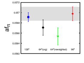
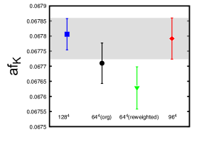
Figure 12: Same as Fig. 10, but for decay constants of pion (left) and kaon (right) in lattice units.

Finally, we compare our results of $f_{K}/f_{\pi}=1.1898(26)(^{+0}_{-1})$ with the FLAG average value of $f_{K^{\pm}}/f_{\pi^{\pm}}$. To this end, we follow the prescription to estimate the strong-isospin correction based on NLO SU(3) ChPT FlavourLatticeAveragingGroupFLAG:2021npn ,

$$\frac{f_{K^{\pm}}}{f_{\pi^{\pm}}} = \frac{f_{K}}{f_{\pi}}\sqrt{1+\delta_{\rm SU(2)}},$$ (33)

$$\delta_{\rm SU(2)} \approx \sqrt{3}\,\epsilon_{\rm SU(2)}\left[-\frac{4}{3}\left(f_{K}/f_{\pi}-1\right)+\frac{2}{3(4\pi)^{2}f_{0}^{2}}\left(m_{K}^{2}-m_{\pi}^{2}-m_{\pi}^{2}\ln\frac{m_{K}^{2}}{m_{\pi}^{2}}\right)\right]\,.$$ (34)

Using $\epsilon_{\rm SU(2)}=\sqrt{3}/(4R)$ with $R=38.1(1.5)$, $F_{0}=f_{0}/\sqrt{2}=80(20)$ MeV FlavourLatticeAveragingGroupFLAG:2021npn and the values of $m_{\pi},m_{K}$ determined in Sec. VII, we estimate $\delta_{\rm SU(2)}\simeq-0.0038$ and obtain

$$\frac{f_{K^{\pm}}}{f_{\pi^{\pm}}} = 1.1875(26)(^{+0}_{-1})(23),$$ (35)

where the error in the third parenthesis is due to 100% uncertainty assumed for $\delta_{\rm SU(2)}$. This result is found to be consistent with the FLAG average value for $(2+1)$-flavor QCD, $f_{K^{\pm}}/f_{\pi^{\pm}}=1.1917(37)$ FlavourLatticeAveragingGroupFLAG:2021npn within uncertainties.

V Stable Baryons

In this section, we calculate the masses of the five baryons, $N$, $\Lambda$, $\Sigma$, $\Xi$, and $\Omega$, which are low-lying stable baryons in strong interaction. The obtained result for the $\Omega$ mass will be used for the scale setting in Sec. VII.

V.1 Calculation strategy

The mass of a baryon $B$ is calculated from two-point temporal correlators,

$$C(\tau)=\sum_{{\vec{x}}}\langle B^{\rm(sink)}({\vec{x}},\tau)\overline{B}^{\rm(src)}(\vec{y},0)\rangle,$$ (36)

where we omit the spin indices for simplicity.

The baryon operator $B(x)$ with $x=(\vec{x},\tau)$ for an octet baryon is defined by

$$B(x)=\epsilon^{abc}(q_{a}(x)^{T}C\gamma_{5}q_{b}(x))q_{c}(x),$$ (37)

where $C=\gamma_{4}\gamma_{2}$ is the charge conjugation matrix and $a,b,c$ are the color indices. The spin and parity projection to $J^{P}=\frac{1}{2}^{+}$ is performed as

$$C^{({\rm O})}(\tau)={\rm Tr}\left[P^{\frac{1}{2}^{+}}C(\tau)\right]$$ (38)

with

$$P^{\frac{1}{2}^{+}}\equiv\frac{1+\gamma_{4}}{2},$$ (39)

where ${\rm Tr}$ is taken in the spinor space.

For the decuplet baryons with spin $3/2$, we employ the correlator of the Rarita-Schwinger fields defined as

$$C_{ij}(\tau) = \sum_{{\vec{x}}}\langle B^{\rm(sink)}_{i}({\vec{x}},\tau)\overline{B}^{\rm(src)}_{j}(\vec{y},0)\rangle,$$ (40)

$$B_{i}(x) = \epsilon^{abc}(q_{a}(x)^{T}C\gamma_{i}q_{b}(x))q_{c}(x),$$ (41)

where we explicitly show the indices for the spatial label of the Rarita-Schwinger fields, $i,j=1,2,3$. The spin and parity projection to $J^{P}=\frac{3}{2}^{+}$ is performed as

$$C^{({\rm D})}(\tau)=\sum_{\begin{subarray}{c}i,j=1,2,3\end{subarray}}{\rm Tr}\left[P_{ij}^{\frac{3}{2}^{+}}C_{ij}(\tau)\right]$$ (42)

with

$$P_{ij}^{\frac{3}{2}^{+}}\equiv\frac{1+\gamma_{4}}{2}(\delta_{ij}-\frac{1}{3}\gamma_{i}\gamma_{j}).$$ (43)

In the calculation of the correlators, there is additional freedom to introduce smearing in the sink and/or source quark operators. After benchmark of several possibilities, we employ the analysis of the correlators with the point-sink and wall-source operators as our main results, where the quark operator in the source operator $B^{\rm(src)}$ is replaced with the wall-source one,

$$q^{({\rm w})}_{a}(\tau)\equiv\sum_{\vec{y}}q_{a}({\vec{y}},\tau),$$ (44)

together with the Coulomb gauge fixing for the configurations. A reason for this choice is that the large amount of statistical data is accumulated for this setup as the by-product of our calculations of two-baryon systems with the wall-source, and we can achieve better precision compared to other choices.

In the case of the mass of $\Omega$, which is obtained with the highest precision and is used for the scale setting, we perform additional calculations using the variational method Luscher:1990ck with the smeared-sink and smeared-source operators. In this method, a rigorous upper bound for the mass can be obtained, and we can estimate the systematic error in the result obtained from the wall-source.

In the variational method, a generalized eigenvalue problem (GEVP) is solved for the correlator matrix of the baryon. The $(l,l^{\prime})$-element of the correlator matrix is defined as the two-point temporal correlators with $l$-th smeared-sink and $l^{\prime}$-th smeared-source operators

$$\left[C(\tau)\right]_{ll^{\prime}}=\sum_{\vec{x}}\langle B^{(l)}(\vec{x},\tau)\overline{B}^{(l^{\prime})}(\vec{y},0)\rangle.$$ (45)

Here, the smeared baryon operators, $B^{(l)}$, are given by replacing the local quark operator with the smeared one,

$$q^{(l)}_{a}({\vec{x}},\tau)=\sum_{\vec{y}}f_{q}^{(l)}(|{\vec{x}}-{\vec{y}}|)q_{a}({\vec{y}},\tau),$$ (46)

where $f_{q}^{(l)}(r)$ is a smearing function.

The GEVP of the correlator matrix is solved as

$$\tilde{C}(\tau)=V^{\dagger}(\tau_{D})C^{-1/2}(\tau_{0})C(\tau)C^{-1/2}(\tau_{0})V(\tau_{D})$$ (47)

with the parameter $\tau_{0}$ and $\tau_{D}$, and the rotational matrix $V(\tau_{D})$ is defined to make the matrix $\tilde{C}(\tau_{D})$ diagonal. It is also checked that $\tilde{C}(\tau)$ at $\tau\neq\tau_{D}$ is almost diagonal. The component $[\tilde{C}(\tau)]_{11}$ corresponds to the correlator of the lowest energy state. The parameters $\tau_{0}$ and $\tau_{D}$ with $\tau_{D}>\tau_{0}\geq\tau/2$ Blossier:2009kd should be large to suppress the contribution from the excited states.

For the calculation of the correlators with smeared-sink and smeared-source, we utilize the $Z_{3}$ noise source method PhysRevD.82.114501 ; PhysRevD.88.014503 ; Wu_2018 ; PACS:2019ofv in order to reduce the statistical fluctuations. The three-dimensional lattice of size $L^{3}$ is divided into $n_{\rm sub}^{3}$ sub-lattices with the size of $L_{\rm sub}^{3}=(L/n_{\rm sub})^{3}$, and the sub-lattices are labeled by the even-odd coloring. The spatial center of the smearing function $f_{q}^{(l)}$ is located on each even-colored sub-lattice so that $(n_{\rm sub}^{3}/2)$ copies of the original smearing function are distributed in the total lattice, and each copy of the smearing function is multiplied by the $Z_{3}$ random number. In this way, we can prepare a quark source operator which has support for an independent single-baryon operator at $(n_{\rm sub}^{3}/2)$ spatially different places simultaneously. The spatial distribution of this work is same as the $s2$ (even-odd) spatial dilution (in sub-lattice degrees of freedom) given in Ref. Akahoshi:2019klc , and also as the crystal structure of face-centered-cubic (FCC) in Ref. PACS:2019ofv .

In our study, we employ a Gaussian-type smearing function. Moreover, we use the tail-cut technique for the smearing, where the smearing function is defined within a finite distance in order to avoid overlap of the smearing functions from spatially separated sources. The explicit form for the smearing function in Eq. (46) is given as

$$f_{q}^{(l)}(r)=\begin{cases}A_{q}^{(l)}{\rm e}^{-\alpha_{q}^{(l)}r^{2}}\quad&\text{for}\ 0<r<r_{\rm cut},\\ 1\quad&\text{for}\ r=0,\\ 0\quad&\text{for}\ r_{\rm cut}\leq r.\end{cases}$$ (48)

When combined with the $Z_{3}$ noise source method on our lattice with $L/a=96$, we take $L_{\rm sub}/a=24$ with $n_{\rm sub}=4$ so that $n_{\rm sub}^{3}/2=32$ single baryon sources are distributed on the lattice (i.e., at spacial locations of $(0,0,0),(48,0,0),(24,24,0),(72,24,0),(0,48,0),(48,48,0),(24,72,0),(72,72,0),(24,0,24),\cdots,(48,72,72)$), and the tail-cut parameter is taken as $r_{\rm cut}=L_{\rm sub}/(\sqrt{2}a)$. We confirm that both the $Z_{3}$ noise method and the tail-cut technique improve the signal-to-noise of the results of the baryon masses.

We have performed benchmark calculations with relatively low statistics to tune the dimension of the correlator matrix (from $2\times 2$ to $5\times 5$) and the smearing parameters. In general, the lowest eigenstate of the correlator matrix is expected to have a larger overlap with the desired ground state if the matrix has a larger size. However, we found that the statistical error increases with the size of the correlator matrix. Finally, we employ the $2\times 2$ correlator matrix in our study with high statistics to obtain the clearest signal of the $\Omega$ baryon mass. The corresponding two sets of the smearing parameters for the $s$-quark sector $(q=s)$ are taken as $A_{s}^{(1)}=A_{s}^{(2)}=1$, $(\alpha_{s}^{(1)},\alpha_{s}^{(2)})=(0.30250,0.02560)$, where the smearing parameters of $l=1,2$ correspond to the narrow and broad extent of the quark fields, respectively. The mass of $\Omega$ is obtained by solving GEVP of the corresponding $2\times 2$ correlator matrix.

We also performed supplemental calculations for other baryons in the $2\times 2$ variational method using the smearing parameters for the $u,d$-quark sectors, $A_{u,d}^{(1)}=A_{u,d}^{(2)}=1$, $(\alpha_{u,d}^{(1)},\alpha_{u,d}^{(2)})=(0.13505,0.01155)$, whereas the parameters for the $s$-quark are taken to be the same as in the $\Omega$ case. However, we found that the statistical fluctuations are much larger than the case of $\Omega$. Considering that the computational cost is also much larger due to the $u,d$-quark solver, we do not use the variational method for baryons other than $\Omega$.

V.2 Numerical results: baryon masses

First, we present analyses of the masses of baryons from the correlators with the point-sink and wall-sources. Quark propagators are solved with the periodic boundary condition for all directions and stopping conditions $|r_{\rm crit}|<10^{-8}(10^{-12})$ for $u,d$-quarks ($s$-quark). The hypercubic symmetry on the lattice (4 rotations and 96 temporal source locations) is used with 1600 configurations as well as the average of the forward/backward propagations, so that the total number of measurements is $1600\times 4\times 96\times 2=1,228,800$. The statistical errors are estimated by the jackknife method with 20 jackknife samples (${\rm bin~{}size}=80$ configurations). We have checked that the results are almost unchanged in the case of ${\rm bin~{}size}=160,40,20$ configurations.

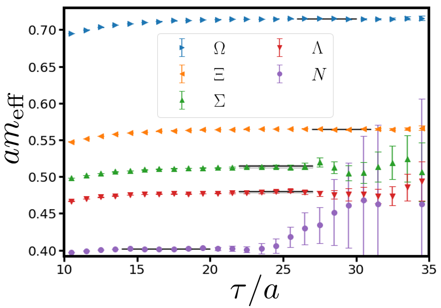
Figure 13: The effective masses for five baryons in lattice units. The fit range and fit results with statistical errors are shown by black lines with gray bands.

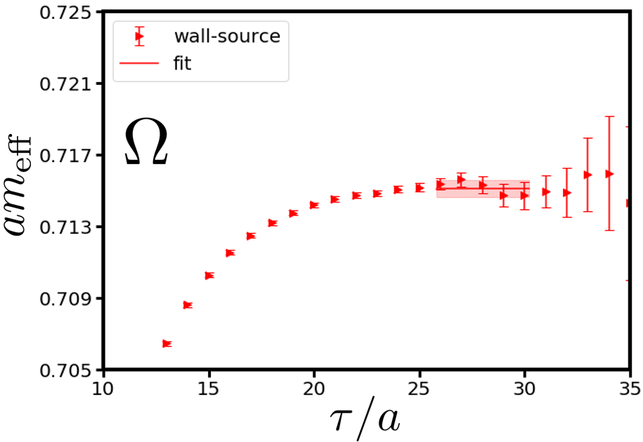
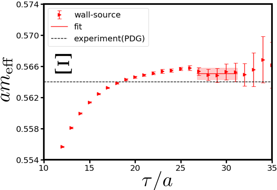
Figure 14: Effective masses for five low-lying baryons with point-sink and wall-source correlators in lattice units. The red lines are the fit results with the red bands denoting the statistical errors. The dotted lines denote the isospin-averaged experimental results from Particle Data Group(PDG) Workman:2022ynf , where the $\Omega$ mass is used for the scale setting.

In Fig. 13, we show the effective masses of five baryons simultaneously, and the enlarged figures for each baryon are shown in Fig. 14, where the effective mass is defined as

$$m_{\rm eff}(\tau)\equiv\log\frac{C^{(B)}(\tau)}{C^{(B)}(\tau+1)}$$ (49)

with $C^{(B)}(\tau)=C^{(O)}(\tau)$ or $C^{(D)}(\tau)$. We observe a good plateau for each baryon corresponding to the ground state saturation.

The baryon masses are obtained by fitting the correlators by a single exponential functional form with the fit ranges chosen from the plateau regions in the effective mass plots. In Figs. 13 and 14, the fit results are shown by black lines with gray bands denoting the statistical errors. The numerical fit results with statistical errors and the fit ranges are summarized in Table 5. We also consider several different choices for the fit ranges by changing the lower and/or upper bounds of ranges by several time slices, and estimate the systematic errors in the baryon masses. The resulting systematic errors for the octet baryons are given in Table 5. The relative magnitudes of the finite volume effect are expected to be $\sim(m_{\rm PS}/m_{B})\cdot e^{-(m_{\rm PS}L)}/(m_{\rm PS}L)<{\cal O}(10^{-4})$ from ChPT with $m_{\rm PS}(m_{B})$ being a relevant PS meson mass (baryon mass) Gasser:1987zq , and thus are negligible in the current precision. In the case of the $\Omega$ mass, the systematic errors are estimated not only from the fit range dependence but also from the analysis with the variational method as will be described below. This additional study is performed because the $\Omega$ mass is determined with the highest precision and is used for the scale setting.

Table 5: The results of the masses of the five baryons in lattice unit. The central values as well as statistical errors (in the first parentheses) are obtained from the analyses of the wall-source data with the fit ranges given in the table. The systematic errors (in the second parentheses) are estimated from the fit range dependence. In the case of the $\Omega$ mass, the result of the variational method is additionally used to estimate the systematic error.

baryon	mass	fit range
$N$	$0.40179(64)(^{+4}_{-20})$	[14,20]
$\Lambda$	$0.47947(154)(^{+18}_{-95})$	[22,27]
$\Sigma$	$0.51414(237)(^{+11}_{-105})$	[22,27]
$\Xi$	$0.56469(74)(^{+58}_{-0})$	[27,31]
$\Omega$	$0.71510(46)(^{+93}_{-5})$	[26,30]

We present the details of the analysis with the variational method for the $\Omega$ baryon. The $2\times 2$ correlator matrix is calculated with the $Z_{3}$ noise method and the tail-cut technique at 16 temporal source locations, and thus the total number of measurements is $1600\ \mbox{confs}\times 4\ \mbox{rotations}\times 16\ \mbox{sources}\times 2\ \mbox{propagations}=204,800$. The statistical errors are estimated by the jackknife method with ${\rm bin~{}size}=80$ configurations as in the case of the wall-source analysis and bin size dependence is found to be negligible. In terms of the parameters in the variational method, $\tau_{0}$ and $\tau_{D}$ in Eq. (47), we tried several combinations and $(\tau_{0},\tau_{D})=(19,22)$ is found to give the clearest signal for the $\Omega$ baryon.

The effective mass of $\Omega$ with the variational method is shown in Fig. 15 by blue circles. Here, the effective mass is defined by

$$\tilde{m}_{\rm eff}(\tau)=-\frac{1}{\tau-\tau_{0}}\log[\tilde{C}(\tau)]_{11}$$ (50)

with $[\tilde{C}(\tau)]_{11}$ being the lowest diagonal element of Eq. (47). This definition is found to give smaller statistical errors than the case of Eq. (49). Shown together in Fig. 15 by red triangles are the effective masses from the point-sink and wall-source (with the definition of Eq. (49) as before). We find that the results from the variational method and the wall-source converge to consistent plateaux within the error bars around $26\lesssim\tau/a\lesssim 30$. By fitting $[\tilde{C}(\tau)]_{11}$ with a single exponential function, we obtain the result of the variational method as $am_{\Omega}^{({\rm var.})}=0.71603(120)$ with the fit range $[26,30]$. The result is insensitive to a change of the fit range.

We note that the result from the variational method gives us the upper bound of the true value, while that from the wall-source analysis does not have such a property. In our analysis, we see that the $\Omega$ mass from the variational method decreases as the parameters $(\tau_{0},\tau_{D})$ increase. However, the statistical error is found to become larger in the case of larger $(\tau_{0},\tau_{D})$. This is why we employ $(\tau_{0},\tau_{D})=(19,22)$ as an optimal choice in the variational method and we utilize the corresponding result to estimate the upper side of the systematic error for the $\Omega$ mass.

Our final result for the $\Omega$ mass leads to $am_{\Omega}=0.71510(46)(^{+93}_{-5})$ and is given in Table 5. The central value and statistical error are obtained from the wall-source analysis. The systematic error is estimated from the largest deviation considering both the upper bound given from the variational method and the fit range dependence in the wall-source analysis.

In the study of the PACS Collaboration, which employs essentially the same configuration setup as this study, any reasonable plateau is not found for $\Omega$ in their point-sink and (exponential-type) smeared-source two-point correlator PACS:2019ofv . A possible reason why we observe a clear plateau in our point-sink and wall-source correlator is that excited state contaminations from meson-baryon scattering states are expected to be suppressed in the wall-source because the dominant meson-baryon states are the P-wave states. We also note that our statistics are much larger than those in Ref. PACS:2019ofv , which is helpful in identifying the plateau.

In the variational method, such excited state contaminations are automatically suppressed by solving the GEVP. However, we employ only single-baryon (three-quark) type operators in our variational method, which would have a small overlap with meson-baryon scattering states. This could be a reason why we have to take large $(\tau_{0},\tau_{D})$ in our study. In the future, it will be desirable to employ not only single-baryon type operators but also meson-baryon type operators in the variational method.

Figure 15: The effective mass for $\Omega$ baryon in lattice units with two analyses, one from the point-sink and wall-source operators (red triangles) and the other from the variational method (blue circles). The fit results as well as the corresponding statistical errors for each analysis are shown by lines and bands, respectively. The data are slightly shifted horizontally for visibility.

VI Unstable hadrons

We present the study of the low-lying resonances, the decuplet baryons ($\Delta,\Sigma^{*}~{}\rm{and}~{}\Xi^{*}$), and the vector mesons ($\rho,K^{*}~{}\rm{and}~{}\phi$). As a rigorous treatment of these hadrons, it is necessary to calculate the scattering phase shifts of the relevant decay modes as formulated in Refs. Luscher:1990ux ; Ishii:2006ec and extract the pole position in the scattering matrix. Since such a detailed analysis is beyond the scope of this paper, we here present a simple analysis which is performed in the same way as in the case of stable hadrons. Such an analysis is expected to be a good approximation for hadrons with small decay widths, but large systematic uncertainties are introduced for hadrons with large decay widths.

The correlators are calculated with the point-sink and wall-source operators as described in Sec. V.2. The effective mass plots are shown in Appendix C. The fit results are summarized in Table 6. We note again that the study considering decay modes is necessary in the future in particular for hadrons with large decay widths.

Table 6: The results of the masses of the resonant hadrons in lattice units. The central values as well as statistical errors (in the first parentheses) are obtained from the analyses of the wall-source data with the fit ranges given in the table. The systematic errors (in the second parentheses) are estimated from the fit range dependence.

hadron	mass	fit range
$\Delta$	$0.54195(105)(^{+7}_{-4})$	[11,16]
$\Sigma^{*}$	$0.60080(417)(^{+115}_{-0})$	[20,24]
$\Xi^{*}$	$0.66178(175)(^{+0}_{-211})$	[25,28]
$\rho$	$0.31710(8)(^{+36}_{-4147})$	[6,10]
$K^{*}$	$0.38156(8)(^{+6}_{-604})$	[11,15]
$\phi$	$0.43695(8)(^{+1}_{-33})$	[19,25]

VII Scale setting and observables in physical units

The lattice cutoff scale is determined in this section. In our study, we choose the mass of the $\Omega$ baryon, $m_{\Omega}$, for the determination of the lattice cutoff scale. As was shown in Sec. V.2, $m_{\Omega}$ is determined with the highest precision among all the baryons considered and its systematic error is thoroughly under control.

Using the experimental value of the $\Omega$ mass Workman:2022ynf , $m_{\Omega}=1672.45\ [{\rm MeV}],$ we determine the lattice spacing as

$$a =0.084372(54)(^{+109}_{-6})\ [{\rm fm}],$$ (51)

$$\frac{1}{a} =2338.8(1.5)(^{+0.2}_{-3.0})\ [{\rm MeV}].$$ (52)

We also confirm that the lattice scale determined from the $\Xi$ mass is consistent with that from the $\Omega$ mass. Our lattice scale is slightly different from that obtained from PACS10 configurations PACS:2019ofv , which employ essentially the same gauge configuration setup, $a^{-1}_{\rm PACS10}=2316.2(4.4)\ [{\rm MeV}]$. For in-depth comparison between two results, see Appendix B.

Using our lattice cutoff scale, we can now give the physical values for the renormalized quark masses and the decay constants of PS mesons as

$$m_{ud}^{\overline{\rm MS}}(\mbox{2 GeV})=3.225(^{+16}_{-19})(46)\ [{\rm MeV}],\quad m_{s}^{\overline{\rm MS}}(\mbox{2 GeV})=88.37(^{+0.15}_{-0.22})(1.26)\ [{\rm MeV}],$$ (53)

$$f_{\pi}=133.3(^{+0.4}_{-0.5})(1.6)\ [{\rm MeV}],\quad f_{K}=158.6(^{+0.3}_{-0.4})(1.9)\ [{\rm MeV}].$$ (54)

Here, the first errors denote the sum of the statistical and systematic errors of each quantity in lattice units as well as the statistical and systematic errors of the lattice unit combined in quadrature, while the second errors in quark masses and decay constants present the error of $(Z_{A}/Z_{P})$ and $Z_{A}$, respectively.

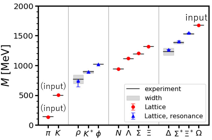
Figure 16: Summary of hadron spectrum at the physical point, where $m_{\Omega}$ is used as an input for the scale setting. $m_{\pi},m_{K}$ are outputs in this paper, but they were essentially used as inputs in previous studies with the same lattice setting Ishikawa:2018jee . Red circles and blue triangles denote the masses of stable hadrons and hadronic resonances, respectively, with statistical and systematic errors combined in quadrature. Horizontal black lines denote the experimental values, and gray bands correspond to the decay widths of resonances.

The masses of low-lying hadrons in physical units are given in Table 7. The numbers in the first (second) parentheses denote the statistical (systematic) errors. The statistical correlations between each hadron and $\Omega$ baryon wall-source correlators are properly taken into account in the estimate of statistical errors. In Table 7, the experimental values corresponding to the isospin-averaged masses are also shown for comparison. In Fig. 16, we show a summary plot for stable hadrons by red circles together with experimental values shown by black lines. In this paper, $m_{\Omega}$ is used as an input for the scale setting, and masses of all other hadrons, including $m_{\pi},m_{K}$, are outputs. In Fig. 16, however, we indicate that $m_{\pi},m_{K}$ also correspond to inputs, since quark mass parameters $\kappa_{ud},\kappa_{s}$ used in this study were previously tuned using $m_{\pi},m_{K}$ in Ref. Ishikawa:2018jee .

The lattice results of the masses of hadrons are found to be sufficiently close to the experimental results considering the uncertainties of the isospin breaking effects. This also indicates that the discretization errors in this study is small, but it would be better to perform explicit calculations for the continuum extrapolation in the future. In Fig. 16, the results for hadron resonances are also shown by blue triangles. Note that they are obtained neglecting the effect of hadronic decays and more proper phase shift studies of relevant decay modes are left for future studies.

Table 7: Summary table for the masses of stable hadrons in physical units. The first and second parentheses denote the statistical and systematic errors, respectively. The experimental values correspond to isospin-averaged ones.

hadron	experiment [MeV]	lattice [MeV]
$\pi$	138.04	$137.1(0.3)(^{+0.0}_{-0.2})$
$K$	495.64	$501.8(0.3)(^{+0.0}_{-0.7})$
$N$	938.92	$939.7(1.8)(^{+0.2}_{-1.7})$
$\Lambda$	1115.68	$1121.4(3.6)(^{+0.5}_{-3.7})$
$\Sigma$	1193.15	$1202.5(5.6)(^{+0.3}_{-4.0})$
$\Xi$	1318.29	$1320.7(2.1)(^{+1.5}_{-1.7})$
$\Omega$	1672.45	input

VIII Summary and concluding remarks

In this paper, we have reported the scale setting and hadronic properties for a new set of lattice QCD gauge configurations generated by the HAL QCD Collaboration which is named as “HAL-conf-2023”. The purpose of this new generation is to enable lattice simulations at the physical point, on a large lattice volume and with a large number of ensembles. We employed $(2+1)$-flavor nonperturbatively ${\cal O}(a)$ improved Wilson fermions with stout smearing and the Iwasaki gauge action at $\beta=1.82$. The size of the lattice is $96^{4}$, corresponding to $(8.1{\rm fm})^{4}$ in physical units. We generated as many as 8,000 trajectories at the physical point using the simulation parameters employed by the PACS Collaboration Ishikawa:2018jee ; PACS:2019ofv .

We showed the MD history of the generation and basic properties of the configurations including the plaquette value, the topological charge distribution and their auto-correlation times. We observed that the MD evolution was stable, and the auto-correlation times are short even for the topological charge, indicating that this configuration set is well spread in the configuration space.

We performed the scale setting using the $\Omega$ baron mass as a reference scale. The systematic error has been carefully examined by the operator dependence of the correlation function of $\Omega$, and the value of the lattice cutoff is determined as $a^{-1}=2338.8(1.5)(^{+0.2}_{-3.0})$ MeV.

We calculated the correlation functions of hadrons and obtained the physical results of single hadron spectra, quark masses and decay constants of pseudoscalar mesons in the light quark sector. The masses of the pseudoscalar mesons are found to be $(m_{\pi},m_{K})=(137.1(0.3)(^{+0.0}_{-0.2}),501.8(0.3)(^{+0.0}_{-0.7}))$ MeV, which are sufficiently close to the experimental values considering the uncertainties of the isospin breaking. The masses of other stable hadrons also agree with the experimental values within a sub-percent level. The results of the quark masses and decay constants are compared to those from PACS10 configuration with the same simulation parameter Ishikawa:2018jee ; PACS:2019ofv and those of FLAG average FlavourLatticeAveragingGroupFLAG:2021npn , and are found to be consistent within uncertainties. These results show that this configuration set, HAL-conf-2023, serves as good physical point ensembles to be used for future lattice QCD calculations for various physical quantities. One of the notable utilities of HAL-conf-2023 is the physical point simulations of hadron interactions, which are currently in progress and will be reported elsewhere.

Finally, we remark several uncertainties to be investigated in the future. The present calculation is performed at only one lattice spacing and the continuum limit is yet to be taken. While the agreements of our results with experimental values as well as with the FLAG average values (in the continuum limit) indicate that the scaling violation is suppressed for this configuration set, explicit calculations at finer lattice spacings would be desirable. In addition, the “physical point” in our $(2+1)$-flavor lattice QCD simulation is defined only up to the uncertainties of the isospin breaking effects. The vacuum polarization effect of the charm quark has not been taken into account, either. In the future, it is desirable to perform $(2+1+1)$, $(1+1+1)$ and $(1+1+1+1)$-flavor QCD (+ QED) simulations to fully control the systematics in lattice calculations.

Appendix A The ratio-difference method for quark masses

In order to obtain physical quark masses, the so-called ratio-difference method was developed by the BMW Collaboration BMW:2010skj . In this method, AWI and VWI bare quark masses are combined in a different way than the one used in the main text (Sec. IV.1), considering that physical quark masses are obtained by additive and multiplicative (only multiplicative) renormalization for VWI (AWI) masses for Wilson-type fermions.

While their concept and the derivation were well-described in BMW:2010skj , we find that the obtained formula in Ref. BMW:2010skj has to be corrected. This is because they performed the ${\cal O}(ma)$ improvement for AWI masses in each flavor (Eq. (11.6) in Ref. BMW:2010skj ), while such improvement is valid only for flavor non-singlet sectors Bhattacharya:2005rb . In this appendix, we give a formula derived with the correct ${\cal O}(ma)$ improvement. In addition, we take into account the ${\cal O}(g_{0}^{4})$ terms which are neglected in Ref. BMW:2010skj .

We define the AWI bare quark masses as

$$m_{f}^{\rm AWI}+m_{g}^{\rm AWI}=\frac{\langle 0|\partial_{4}A_{4}|PS\rangle}{\langle 0|P|PS\rangle}.$$ (55)

and the VWI bare quark masses

$$m_{f}^{\rm VWI}=\frac{1}{a}\left(\frac{1}{2\kappa_{f}}-\frac{1}{2\kappa_{c}}\right).$$ (56)

Here, ${\cal O}(a)$ improvement of the axial-current $A_{4}\rightarrow A_{4}+ac_{A}\partial_{4}P$ is implicitly understood, and the flavor indices $f,g$ should be taken such that the axial-current is flavor non-singlet.

The physical quark masses $\hat{m}_{f}$ obtained by the ${\cal O}(ma)$ improvement and renormalization for the AWI or VWI bare quark masses are given by Bhattacharya:2005rb

$$\hat{m}_{fg} = \frac{Z_{A}}{Z_{P}}\left[\frac{1+ab_{A}m_{fg}+a\bar{b}_{A}{\rm Tr}M}{1+ab_{P}m_{fg}+a\bar{b}_{P}{\rm Tr}M}\right]m_{fg}^{{\rm AWI}}+{\cal O}(a^{2}),$$ (57)

where $m^{\prime}_{fg}=(m^{\prime}_{f}+m^{\prime}_{g})/2$ with $m^{\prime}$ denoting $\hat{m},m$ or $m^{\rm AWI}$, and

$$\hat{m}_{f} = Z_{m}\left\{\left[m_{f}+(r_{m}-1)\frac{{\rm Tr}M}{N_{f}}\right]\right.$$

$$\qquad\left.+a\left[b_{m}m_{f}^{2}+\bar{b}_{m}m_{f}{\rm Tr}M+(r_{m}d_{m}-b_{m})\frac{{\rm Tr}(M^{2})}{N_{f}}+(r_{m}\bar{d}_{m}-\bar{b}_{m})\frac{({\rm Tr}M)^{2}}{N_{f}}\right]\right\}+{\cal O}(a^{2}).$$

In the following, we employ $m^{\rm VWI}$ for the bare mass $m$ appearing in the ${\cal O}(ma)$ improvement terms as is usually the case in the literature Bhattacharya:2005rb , and the improvement coefficients, $b_{X},\bar{b}_{X},d_{X},\bar{d}_{X}(X=A,P,m)$, are defined accordingly.

We now derive the formula for the ratio-difference method. For simplicity, we consider $N_{f}=2+1$ QCD hereafter, with flavor indices $(u,d,s)$ labeled by $(1,2,3)$. The formula for other flavor cases can be obtained similarly.

We begin with the following definitions and trivial equalities,

$$d^{\rm imp} \equiv \frac{1}{Z_{m}}(a\hat{m}_{s}-a\hat{m}_{ud})$$ (59)

$$d \equiv am_{s}^{{\rm VWI}}-am_{ud}^{{\rm VWI}}$$ (60)

$$r^{\rm imp} \equiv \frac{\hat{m}_{s}}{\hat{m}_{ud}}$$ (61)

$$r \equiv \frac{m_{s}^{{\rm AWI}}}{m_{ud}^{{\rm AWI}}}=2\frac{m_{13}^{{\rm AWI}}}{m_{12}^{{\rm AWI}}}-1$$ (62)

$$a\hat{m}_{ud} = Z_{m}\frac{d^{\rm imp}}{r^{\rm imp}-1}$$ (63)

$$a\hat{m}_{s} = Z_{m}\frac{r^{\rm imp}d^{\rm imp}}{r^{\rm imp}-1}$$ (64)

From Eqs. (57) and (LABEL:eq:VWI-mass-phys-each),

$$d^{\rm imp} = (am_{s}^{{\rm VWI}}-am_{ud}^{{\rm VWI}})\times\left[1+ab_{m}(m_{s}^{{\rm VWI}}+m_{ud}^{{\rm VWI}})+a\bar{b}_{m}{\rm Tr}M^{\rm VWI}+{\cal O}(a^{2})\right]$$ (65)

$$\frac{\hat{m}_{13}}{\hat{m}_{12}} = \frac{1}{2}r^{\rm imp}+\frac{1}{2}$$ (66)

$$= \frac{m_{13}^{{\rm AWI}}}{m_{12}^{{\rm AWI}}}\left[1+a(b_{A}-b_{P})(m_{13}^{{\rm VWI}}-m_{12}^{{\rm VWI}})+{\cal O}(a^{2})\right]$$

$$= \frac{r+1}{2}\left[1+(b_{A}-b_{P})\frac{1}{2}d+{\cal O}(a^{2})\right]$$

The next step is to express $(m_{s}^{{\rm VWI}}+m_{ud}^{{\rm VWI}})$ and ${\rm Tr}M^{\rm VWI}=(m_{s}^{{\rm VWI}}+2m_{ud}^{{\rm VWI}})$ which appear in $d^{\rm imp}$ by some functions of $r,d$. For this purpose, we use Eqs. (66) and (LABEL:eq:VWI-mass-phys-each) to show that

$$\frac{\hat{m}_{s}}{\hat{m}_{ud}} = r+{\cal O}(a)$$ (67)

and

$$\frac{\hat{m}_{s}}{\hat{m}_{ud}} = \frac{m_{s}^{{\rm VWI}}+(r_{m}-1)\frac{1}{3}(m_{s}^{{\rm VWI}}+2m_{ud}^{{\rm VWI}})}{m_{ud}^{{\rm VWI}}+(r_{m}-1)\frac{1}{3}(m_{s}^{{\rm VWI}}+2m_{ud}^{{\rm VWI}})}+{\cal O}(a).$$ (68)

Equating Eqs. (67) and (68), we obtain

$$\frac{m_{s}^{{\rm VWI}}}{m_{ud}^{{\rm VWI}}} = \frac{(2r_{m}+1)r-2(r_{m}-1)}{(r_{m}+2)-(r_{m}-1)r}+{\cal O}(a)$$ (69)

and thus

$$am_{s}^{{\rm VWI}}+am_{ud}^{{\rm VWI}} = (am_{s}^{{\rm VWI}}-am_{ud}^{{\rm VWI}})\cdot\frac{m_{s}^{{\rm VWI}}/m_{ud}^{{\rm VWI}}+1}{m_{s}^{{\rm VWI}}/m_{ud}^{{\rm VWI}}-1}$$ (70)

$$= d\left[\frac{3(r+1)+(r_{m}-1)(r-1)}{3r_{m}(r-1)}+{\cal O}(a)\right]$$

$$am_{s}^{{\rm VWI}}+2am_{ud}^{{\rm VWI}} = (am_{s}^{{\rm VWI}}-am_{ud}^{{\rm VWI}})\cdot\frac{m_{s}^{{\rm VWI}}/m_{ud}^{{\rm VWI}}+2}{m_{s}^{{\rm VWI}}/m_{ud}^{{\rm VWI}}-1}$$ (71)

$$= d\left[\frac{r+2}{r_{m}(r-1)}+{\cal O}(a)\right]$$

To summarize, the formula for the ratio-difference method is

$$a\hat{m}_{ud} = Z_{m}\frac{d^{\rm imp}}{r^{\rm imp}-1}$$ (72)

$$a\hat{m}_{s} = Z_{m}\frac{r^{\rm imp}d^{\rm imp}}{r^{\rm imp}-1}$$ (73)

$$d^{\rm imp} = d\cdot\left[1+b_{m}d\cdot\frac{3(r+1)+(r_{m}-1)(r-1)}{3r_{m}(r-1)}+\bar{b}_{m}d\cdot\frac{r+2}{r_{m}(r-1)}+{\cal O}(a^{2})\right]$$ (74)

$$r^{\rm imp} = r\left[1+(b_{A}-b_{P})d\cdot\frac{r+1}{2r}+{\cal O}(a^{2})\right]$$ (75)

$$d = \frac{1}{2\kappa_{s}}-\frac{1}{2\kappa_{ud}}$$ (76)

$$r = 2\frac{m_{13}^{{\rm AWI}}}{m_{12}^{{\rm AWI}}}-1,$$ (77)

where $d^{\rm imp}$ and $r^{\rm imp}$ are different from the original formula given by the BMW Collaboration (Eqs. (11.14) and (11.15) in Ref. BMW:2010skj ).

We note that, in numerical calculations for quark masses by the BMW Collaboration BMW:2010skj ; BMW:2013fzj , the tree-level improvement coefficients are used in practice, where $(b_{A}-b_{P})=\bar{b}_{A}=\bar{b}_{P}=\bar{b}_{m}=0,r_{m}=1$. In such a case, the differences in the formula become irrelevant and their numerical results remain intact.

Appendix B Comparison with PACS10 study

We present a comparison of physical point simulations with our HAL-Conf-2023 configurations and PACS10 configurations by the PACS collaboration Ishikawa:2018jee ; PACS:2019ofv , where the same action with the same parameters such as hopping parameters $\kappa$ (except for the lattice volume) are employed in the generation. More specifically, we find that there is a deviation of $\simeq 1\%$ (corresponding to 4.1$\sigma$) for the obtained values of the lattice cutoff, $a^{-1}_{\rm HAL}=2338.8(1.5)\left({}^{+0.2}_{-3.0}\right)$ MeV in our study and $a^{-1}_{\rm PACS10}=2316.2(4.4)$ MeV in the PACS10 study, and we examine the origin of the difference.

First, we consider the effect of the difference of the lattice volume, where $N_{s}^{4}=96^{4}$ ($L=N_{s}a\simeq 8.1$ fm) in HAL-Conf-2023 and $N_{s}^{4}=128^{4}$ ($L\simeq 10.8$ fm) in PACS10 configurations. In the study of the PACS collaboration Ishikawa:2018jee ; PACS:2019ofv , configurations with $N_{s}^{4}=64^{4}$ ($L\simeq 5.4$ fm) with the same hopping parameters are also generated, and the PS meson masses and the PCAC quark masses are found to be different between $N_{s}=64$ and $N_{s}=128$ due to the finite volume effect on the critical kappa $\kappa_{c}$. On this point, we find that our PS meson masses and PCAC masses in lattice units are consistent with those of PACS10 as shown in Sec. IV.2. This indicates that $N_{s}=96$ is large enough to be compared directly with $N_{s}=128$. In addition, since the PCAC masses (and baryon masses used for the scale setting) in lattice units become larger with a smaller volume in the PACS study, our setup with $N_{s}=96$ might underestimate the cutoff value $a^{-1}$ compared to $N_{s}=128$ due to the finite volume effect on $\kappa_{c}$, if any. This is the opposite effect of the deviation between $a^{-1}_{\rm HAL}$ and $a^{-1}_{\rm PACS10}$. As further consideration, even when finite volume effect on $\kappa_{c}$ is negligible, there could also exist finite volume effect on baryon masses through, e.g., meson cloud contributions. However, such an effect is considered to be negligible for our large spatial volume, as is estimated by ChPT in Sec. V.2 and is numerically demonstrated in the PACS study for the comparison of baryon spectra between $N_{s}=128$ and $N_{s}=64$ (with reweighted $\kappa$ for the latter to compensate for the finite volume effect on $\kappa_{c}$). With these considerations, we conclude that the difference of the lattice volume is not the origin of that between $a^{-1}_{\rm HAL}$ and $a^{-1}_{\rm PACS10}$.

Second, we consider the difference for the definition of the “physical point”. In the PACS10 study, quark masses are slightly reweighted from the simulation point using the experimental values of $(m_{\pi^{0}},m_{K^{0}})$ with the lattice scale determined by $m_{\Xi^{0}}$. On the other hand, we do not use the reweighting since the spectrum on the simulation point is sufficiently close to our physical point target defined by the experimental spectra with the isospin average, $(m_{\pi^{\rm ave}},m_{K^{\rm ave}})$, with the lattice scale determined by $m_{\Omega}$. Among several differences given above, the effect of reweighting on $m_{\Xi^{0}}$ in PACS10 study is much smaller than the difference between $a^{-1}_{\rm HAL}$ and $a^{-1}_{\rm PACS10}$ PACS:2019ofv and can be neglected. Also, the choice of baryon species for the scale setting is not an issue within our study, since the lattice cutoff determined from $m_{\Omega}$ is consistent with that determined from $m_{\Xi^{\rm ave}}$. However, the choice of experimental value for $m_{\Xi}$ does matter. In fact, the experimental value of $m_{\Xi^{0}}$ is about $0.3\%$ smaller than $m_{\Xi^{\rm ave}}$ and thus can explain a part of the $1\%$ deviation between $a^{-1}_{\rm HAL}$ and $a^{-1}_{\rm PACS10}$. Note that this difference is unavoidable uncertainty for the $N_{f}=2+1$ lattice QCD (without QED) simulations, and there is no rigorous theoretical argument which one to choose FlavourLatticeAveragingGroupFLAG:2021npn .

Finally, we examine the origin of the remaining $0.7\%$ deviation for the lattice cutoff. It turns out that the mass of $\Xi$ in lattice units, obtained on the lattice at the simulation point, has 0.5% deviation ($2.6\sigma$) as $(am_{\Xi})_{\rm HAL}=0.56469(74)\left({}^{+58}_{-0}\right)$ and $(am_{\Xi})_{\rm PACS10}=0.56742(50)$. In these calculations, the correlator with the wall-source and point-sink operator is employed in our study, while the smeared-source and point-sink operator is employed in the PACS10 study. In order to further study the dependence on the source operator, we additionally calculate with smeared-source and point-sink operator with two smearing parameter sets, $l=1$ (narrow) and $l=2$ (broad) given in Sec. V.1.

The effective masses in our calculations are shown in Fig.17. The red circles denote the results with the wall-source, and the blue (green) triangles denote those with the narrow (broad) smeared-source. The red horizontal line with a band denotes our fit result obtained from the wall-source with statistical and systematic errors added in quadrature. As Fig.17 shows, all results are consistent with the red band in the large $\tau$ region. In particular, while the wall-source data tend to converge from the lower side, our smeared-source data tend to converge from the upper side, indicating that our identification of the ground state plateau is reliable.

In Fig.17, we also show the result of the PACS10 study for comparison, where the black dashed line with a band is their fit result with their error obtained from the smeared-source at the simulation point. There is a clear deviation from our results as mentioned before. We note that the smearing functions are slightly different between our study and the PACS10 study, and the black dashed line does not correspond to the fit of our smeared-source data (blue and green triangles). Having said that, a comparison implies that, if one analyzes a correlator with only one specific choice of the operator, one may easily misidentify a pseudo-plateau structure at early $\tau$ as a signal of the ground state saturation, which leads to an incorrect result for the spectrum.

As discussed above, our analysis for $m_{\Xi}$ passed the consistency check between different choices of the source operator. In addition, our final result for the lattice cutoff is determined from $m_{\Omega}$, where a more stringent and higher-precision cross check is performed between the result from the wall-source and point-sink operator and that from the variational method with the $2\times 2$ smeared operators (See Sec. V.2). Therefore, we conclude that the reliability of our determination of the lattice cutoff is well established.

Figure 17: Effective mass plot for the $\Xi$ baryon in lattice units with two methods: the point-sink and wall-source operators (red circles) and the point-sink and smeared-source operators (blue (green) triangles for narrow (broad) smearing function). The red horizontal line denotes the fit results with the wall-source and point-sink operator, and the red band denotes the statistical and systematic errors combined in quadrature. The black dashed line with a band denotes the fit result of the PACS10 study, obtained from the smeared-source and point-sink operator at the simulation point PACS:2019ofv .

Appendix C The effective masses of unstable hadrons

We show the effective mass plots for the unstable hadrons (resonances) discussed in Sec. VI. In Fig. 18, the results are shown by red points. Shown together by red lines with red bands are the results of the single-state fit of the correlators with statistical errors. Systematic errors are estimated by the fit range dependence. In some hadrons, we do not see clear single plateaux, and we adopt two separate fit ranges for possible plateaux as explicitly shown in Fig.18.

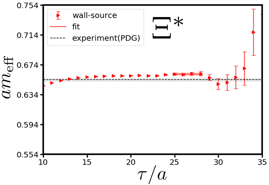
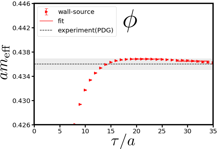
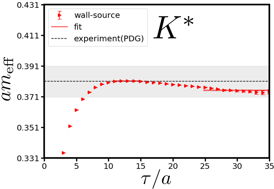
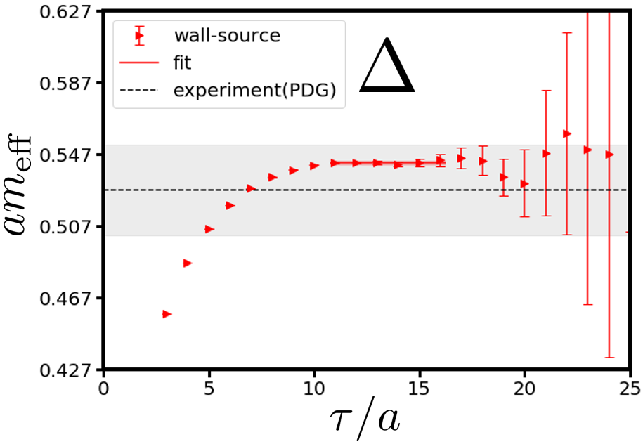
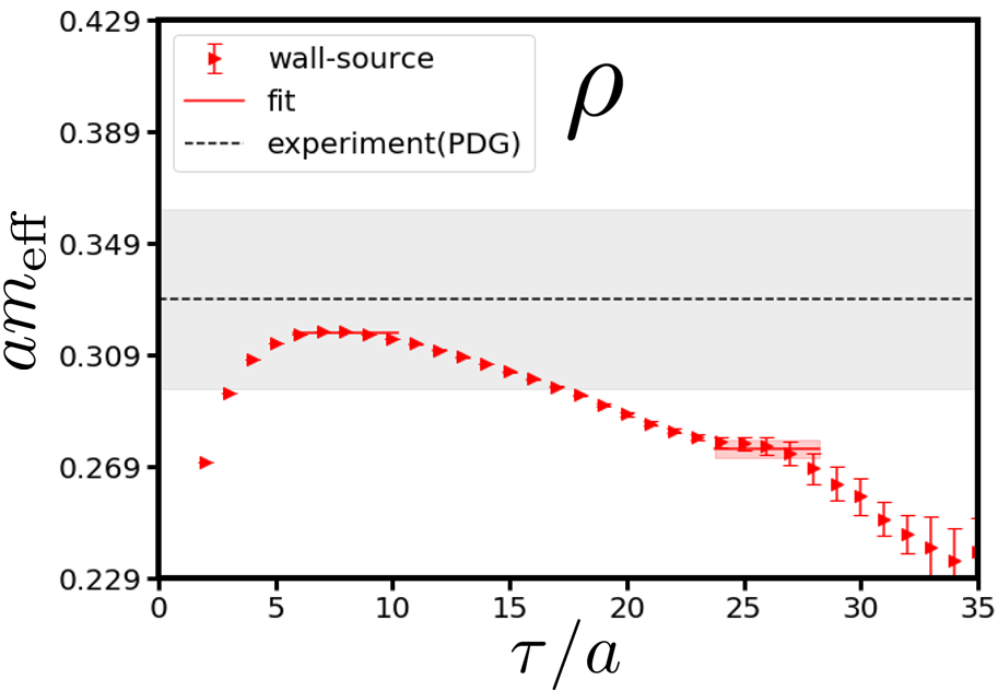
Figure 18: Effective masses for low-lying resonant decuplet baryons and vector mesons with point-sink and wall-source correlators in lattice units. The red lines and red bands denote the fit results and the statistical errors, respectively. The black dotted lines and the gray bands denote the experimental values of masses and widths, respectively.

References

- (1) Flavour Lattice Averaging Group (FLAG) Collaboration, Y. Aoki et al., “FLAG Review 2021,” Eur. Phys. J. C 82 no. 10, (2022) 869, arXiv:2111.09849 [hep-lat].
- (2) T. Aoyama et al., “The anomalous magnetic moment of the muon in the Standard Model,” Phys. Rept. 887 (2020) 1–166, arXiv:2006.04822 [hep-ph].
- (3) S. Borsanyi et al., “Leading hadronic contribution to the muon magnetic moment from lattice QCD,” Nature 593 no. 7857, (2021) 51–55, arXiv:2002.12347 [hep-lat].
- (4) G. Parisi, “The Strategy for Computing the Hadronic Mass Spectrum,” Phys. Rept. 103 (1984) 203–211.
- (5) G. P. Lepage, “The Analysis of Algorithms for Lattice Field Theory,” in Theoretical Advanced Study Institute in Elementary Particle Physics. 6, 1989.
- (6) S. Gongyo et al., “Most Strange Dibaryon from Lattice QCD,” Phys. Rev. Lett. 120 no. 21, (2018) 212001, arXiv:1709.00654 [hep-lat].
- (7) HAL QCD Collaboration, T. Iritani et al., “ dibaryon from lattice QCD near the physical point,” Phys. Lett. B 792 (2019) 284–289, arXiv:1810.03416 [hep-lat].
- (8) HAL QCD Collaboration, K. Sasaki et al., “ and N interactions from lattice QCD near the physical point,” Nucl. Phys. A 998 (2020) 121737, arXiv:1912.08630 [hep-lat].
- (9) Y. Lyu, H. Tong, T. Sugiura, S. Aoki, T. Doi, T. Hatsuda, J. Meng, and T. Miyamoto, “Dibaryon with Highest Charm Number near Unitarity from Lattice QCD,” Phys. Rev. Lett. 127 no. 7, (2021) 072003, arXiv:2102.00181 [hep-lat].
- (10) S. Aoki and T. Doi, “Lattice QCD and baryon-baryon interactions: HAL QCD method,” Front. in Phys. 8 (2020) 307, arXiv:2003.10730 [hep-lat].
- (11) A. Francis, J. R. Green, P. M. Junnarkar, C. Miao, T. D. Rae, and H. Wittig, “Lattice QCD study of the dibaryon using hexaquark and two-baryon interpolators,” Phys. Rev. D 99 no. 7, (2019) 074505, arXiv:1805.03966 [hep-lat].
- (12) B. Hörz et al., “Two-nucleon S-wave interactions at the flavor-symmetric point with : A first lattice QCD calculation with the stochastic Laplacian Heaviside method,” Phys. Rev. C 103 no. 1, (2021) 014003, arXiv:2009.11825 [hep-lat].
- (13) S. Amarasinghe, R. Baghdadi, Z. Davoudi, W. Detmold, M. Illa, A. Parreno, A. V. Pochinsky, P. E. Shanahan, and M. L. Wagman, “Variational study of two-nucleon systems with lattice QCD,” Phys. Rev. D 107 no. 9, (2023) 094508, arXiv:2108.10835 [hep-lat].
- (14) J. R. Green, A. D. Hanlon, P. M. Junnarkar, and H. Wittig, “Weakly bound dibaryon from SU(3)-flavor-symmetric QCD,” Phys. Rev. Lett. 127 no. 24, (2021) 242003, arXiv:2103.01054 [hep-lat].
- (15) N. Ishii, S. Aoki, and T. Hatsuda, “The Nuclear Force from Lattice QCD,” Phys. Rev. Lett. 99 (2007) 022001, arXiv:nucl-th/0611096.
- (16) HAL QCD Collaboration, N. Ishii, S. Aoki, T. Doi, T. Hatsuda, Y. Ikeda, T. Inoue, K. Murano, H. Nemura, and K. Sasaki, “Hadron–hadron interactions from imaginary-time Nambu–Bethe–Salpeter wave function on the lattice,” Phys. Lett. B 712 (2012) 437–441, arXiv:1203.3642 [hep-lat].
- (17) HAL QCD Collaboration, T. Iritani, S. Aoki, T. Doi, T. Hatsuda, Y. Ikeda, T. Inoue, N. Ishii, H. Nemura, and K. Sasaki, “Consistency between Lüscher’s finite volume method and HAL QCD method for two-baryon systems in lattice QCD,” JHEP 03 (2019) 007, arXiv:1812.08539 [hep-lat].
- (18) Y. Lyu, S. Aoki, T. Doi, T. Hatsuda, Y. Ikeda, and J. Meng, “Doubly Charmed Tetraquark Tcc+ from Lattice QCD near Physical Point,” Phys. Rev. Lett. 131 no. 16, (2023) 161901, arXiv:2302.04505 [hep-lat].
- (19) Y. Lyu, T. Doi, T. Hatsuda, Y. Ikeda, J. Meng, K. Sasaki, and T. Sugiura, “Attractive N- interaction and two-pion tail from lattice QCD near physical point,” Phys. Rev. D 106 no. 7, (2022) 074507, arXiv:2205.10544 [hep-lat].
- (20) PACS Collaboration, K. I. Ishikawa, N. Ishizuka, Y. Kuramashi, Y. Nakamura, Y. Namekawa, Y. Taniguchi, N. Ukita, T. Yamazaki, and T. Yoshie, “2+1 Flavor QCD Simulation on a Lattice,” PoS LATTICE2015 (2016) 075, arXiv:1511.09222 [hep-lat].
- (21) Y. Kamiya, K. Sasaki, T. Fukui, T. Hyodo, K. Morita, K. Ogata, A. Ohnishi, and T. Hatsuda, “Femtoscopic study of coupled-channels and interactions,” Phys. Rev. C 105 no. 1, (2022) 014915, arXiv:2108.09644 [hep-ph].
- (22) E. Hiyama, K. Sasaki, T. Miyamoto, T. Doi, T. Hatsuda, Y. Yamamoto, and T. A. Rijken, “Possible lightest Hypernucleus with Modern Interactions,” Phys. Rev. Lett. 124 no. 9, (2020) 092501, arXiv:1910.02864 [nucl-th].
- (23) E. Hiyama, M. Isaka, T. Doi, and T. Hatsuda, “Probing the N interaction through inversion of spin-doublets in N nuclei,” Phys. Rev. C 106 no. 6, (2022) 064318, arXiv:2209.06711 [nucl-th].
- (24) K.-I. Ishikawa, I. Kanamori, H. Matsufuru, I. Miyoshi, Y. Mukai, Y. Nakamura, K. Nitadori, and M. Tsuji, “102 PFLOPS lattice QCD quark solver on Fugaku,” Comput. Phys. Commun. 282 (2023) 108510, arXiv:2109.10687 [hep-lat].
- (25) PACS Collaboration, K. I. Ishikawa, N. Ishizuka, Y. Kuramashi, Y. Nakamura, Y. Namekawa, Y. Taniguchi, N. Ukita, T. Yamazaki, and T. Yoshie, “Finite size effect on pseudoscalar meson sector in 2+1 flavor QCD at the physical point,” Phys. Rev. D 99 no. 1, (2019) 014504, arXiv:1807.06237 [hep-lat].
- (26) PACS Collaboration, K. I. Ishikawa, N. Ishizuka, Y. Kuramashi, Y. Nakamura, Y. Namekawa, E. Shintani, Y. Taniguchi, N. Ukita, T. Yamazaki, and T. Yoshié, “Finite size effect on vector meson and baryon sectors in 2+1 flavor QCD at the physical point,” Phys. Rev. D 100 no. 9, (2019) 094502, arXiv:1907.10846 [hep-lat].
- (27) PACS-CS Collaboration, S. Aoki et al., “2+1 Flavor Lattice QCD toward the Physical Point,” Phys. Rev. D 79 (2009) 034503, arXiv:0807.1661 [hep-lat].
- (28) PACS-CS Collaboration, S. Aoki et al., “Physical Point Simulation in 2+1 Flavor Lattice QCD,” Phys. Rev. D 81 (2010) 074503, arXiv:0911.2561 [hep-lat].
- (29) BMW Collaboration, S. Durr et al., “Ab-Initio Determination of Light Hadron Masses,” Science 322 (2008) 1224–1227, arXiv:0906.3599 [hep-lat].
- (30) BMW Collaboration, S. Borsanyi et al., “Ab initio calculation of the neutron-proton mass difference,” Science 347 (2015) 1452–1455, arXiv:1406.4088 [hep-lat].
- (31) RBC, UKQCD Collaboration, R. Arthur et al., “Domain Wall QCD with Near-Physical Pions,” Phys. Rev. D 87 (2013) 094514, arXiv:1208.4412 [hep-lat].
- (32) RBC, UKQCD Collaboration, T. Blum et al., “Domain wall QCD with physical quark masses,” Phys. Rev. D 93 no. 7, (2016) 074505, arXiv:1411.7017 [hep-lat].
- (33) M. Bruno et al., “Simulation of QCD with N 2 1 flavors of non-perturbatively improved Wilson fermions,” JHEP 02 (2015) 043, arXiv:1411.3982 [hep-lat].
- (34) RQCD Collaboration, G. S. Bali, S. Collins, P. Georg, D. Jenkins, P. Korcyl, A. Schäfer, E. E. Scholz, J. Simeth, W. Söldner, and S. Weishäupl, “Scale setting and the light baryon spectrum in Nf = 2 + 1 QCD with Wilson fermions,” JHEP 05 (2023) 035, arXiv:2211.03744 [hep-lat].
- (35) C. Alexandrou et al., “Simulating twisted mass fermions at physical light, strange and charm quark masses,” Phys. Rev. D 98 no. 5, (2018) 054518, arXiv:1807.00495 [hep-lat].
- (36) MILC Collaboration, A. Bazavov et al., “Lattice QCD Ensembles with Four Flavors of Highly Improved Staggered Quarks,” Phys. Rev. D 87 no. 5, (2013) 054505, arXiv:1212.4768 [hep-lat].
- (37) A. Bazavov et al., “- and -meson leptonic decay constants from four-flavor lattice QCD,” Phys. Rev. D 98 no. 7, (2018) 074512, arXiv:1712.09262 [hep-lat].
- (38) Y. Iwasaki, “Renormalization Group Analysis of Lattice Theories and Improved Lattice Action. II. Four-dimensional non-Abelian SU(N) gauge model,” arXiv:1111.7054 [hep-lat].
- (39) Y. Taniguchi, “Non-perturbative evaluation of for smeared link clover fermion and Iwasaki gauge action,” PoS LATTICE2012 (2012) 236, arXiv:1303.0104 [hep-lat].
- (40) M. Luscher, “Lattice QCD and the Schwarz alternating procedure,” JHEP 05 (2003) 052, arXiv:hep-lat/0304007.
- (41) M. Hasenbusch, “Speeding up the hybrid Monte Carlo algorithm for dynamical fermions,” Phys. Lett. B 519 (2001) 177–182, arXiv:hep-lat/0107019.
- (42) M. Hasenbusch and K. Jansen, “Speeding up lattice QCD simulations with clover improved Wilson fermions,” Nucl. Phys. B 659 (2003) 299–320, arXiv:hep-lat/0211042.
- (43) M. A. Clark and A. D. Kennedy, “Accelerating dynamical fermion computations using the rational hybrid Monte Carlo (RHMC) algorithm with multiple pseudofermion fields,” Phys. Rev. Lett. 98 (2007) 051601, arXiv:hep-lat/0608015.
- (44) J. C. Sexton and D. H. Weingarten, “Hamiltonian evolution for the hybrid Monte Carlo algorithm,” Nucl. Phys. B 380 (1992) 665–677.
- (45) N. Ukita, private communications.
- (46) M. Lüscher, “Properties and uses of the Wilson flow in lattice QCD,” JHEP 08 (2010) 071, arXiv:1006.4518 [hep-lat]. [Erratum: JHEP 03, 092 (2014)].
- (47) ALPHA Collaboration, M. Bruno, S. Schaefer, and R. Sommer, “Topological susceptibility and the sampling of field space in Nf = 2 lattice QCD simulations,” JHEP 08 (2014) 150, arXiv:1406.5363 [hep-lat].
- (48) BMW Collaboration, S. Borsányi, S. Dürr, Z. Fodor, C. Hoelbling, S. D. Katz, S. Krieg, T. Kurth, L. Lellouch, T. Lippert, and C. McNeile, “High-precision scale setting in lattice QCD,” JHEP 09 (2012) 010, arXiv:1203.4469 [hep-lat].
- (49) BMW Collaboration, S. Durr, Z. Fodor, C. Hoelbling, S. D. Katz, S. Krieg, T. Kurth, L. Lellouch, T. Lippert, K. K. Szabo, and G. Vulvert, “Lattice QCD at the physical point: Simulation and analysis details,” JHEP 08 (2011) 148, arXiv:1011.2711 [hep-lat].
- (50) BMW Collaboration, S. Dürr et al., “Lattice QCD at the physical point meets SU(2) chiral perturbation theory,” Phys. Rev. D 90 no. 11, (2014) 114504, arXiv:1310.3626 [hep-lat].
- (51) Y. Kuramashi, M. Fukugita, H. Mino, M. Okawa, and A. Ukawa, “Lattice QCD calculation of full pion scattering lengths,” Phys. Rev. Lett. 71 (1993) 2387–2390.
- (52) T. Bhattacharya, R. Gupta, W. Lee, S. R. Sharpe, and J. M. S. Wu, “Improved bilinears in lattice QCD with non-degenerate quarks,” Phys. Rev. D 73 (2006) 034504, arXiv:hep-lat/0511014.
- (53) In the literature, a similar -improvement formula for the individual quark mass is sometimes employed PACS-CS:2008bkb ; BMW:2010skj . However, such a formula cannot be justified, since individual quark mass contains both flavor singlet and non-singlet component.
- (54) PACS Collaboration, K. I. Ishikawa, N. Ishizuka, Y. Kuramashi, Y. Nakamura, Y. Namekawa, Y. Taniguchi, N. Ukita, T. Yamazaki, and T. Yoshié, “Mass and Axial current renormalization in the Schrödinger functional scheme for the RG-improved gauge and the stout smeared -improved Wilson quark actions.,” PoS LATTICE2015 (2016) 271, arXiv:1511.08549 [hep-lat].
- (55) G. Colangelo, S. Durr, and C. Haefeli, “Finite volume effects for meson masses and decay constants,” Nucl. Phys. B 721 (2005) 136–174, arXiv:hep-lat/0503014.
- (56) N. Ukita, private communication.
- (57) M. Luscher and U. Wolff, “How to Calculate the Elastic Scattering Matrix in Two-dimensional Quantum Field Theories by Numerical Simulation,” Nucl. Phys. B 339 (1990) 222–252.
- (58) B. Blossier, M. Della Morte, G. von Hippel, T. Mendes, and R. Sommer, “On the generalized eigenvalue method for energies and matrix elements in lattice field theory,” JHEP 04 (2009) 094, arXiv:0902.1265 [hep-lat].
- (59) A. Li, A. Alexandru, Y. Chen, T. Doi, S. J. Dong, T. Draper, M. Gong, A. Hasenfratz, I. Horváth, F. X. Lee, K. F. Liu, N. Mathur, T. Streuer, and J. B. Zhang, “Overlap valence on flavor domain wall fermion configurations with deflation and low-mode substitution,” Phys. Rev. D 82 (Dec, 2010) 114501. https://link.aps.org/doi/10.1103/PhysRevD.82.114501.
- (60) QCD Collaboration Collaboration, M. Gong, A. Alexandru, Y. Chen, T. Doi, S. J. Dong, T. Draper, W. Freeman, M. Glatzmaier, A. Li, K. F. Liu, and Z. Liu, “Strangeness and charmness content of the nucleon from overlap fermions on -flavor domain-wall fermion configurations,” Phys. Rev. D 88 (Jul, 2013) 014503. https://link.aps.org/doi/10.1103/PhysRevD.88.014503.
- (61) J.-J. Wu, W. Kamleh, D. B. Leinweber, R. D. Young, and J. M. Zanotti, “Accessing high-momentum nucleons with dilute stochastic sources,” Journal of Physics G: Nuclear and Particle Physics 45 no. 12, (Nov, 2018) 125102. https://dx.doi.org/10.1088/1361-6471/aaeb9e.
- (62) Y. Akahoshi, S. Aoki, T. Aoyama, T. Doi, T. Miyamoto, and K. Sasaki, “ potential in the HAL QCD method with all-to-all propagators,” PTEP 2019 no. 8, (2019) 083B02, arXiv:1904.09549 [hep-lat].
- (63) Particle Data Group Collaboration, R. L. Workman and Others, “Review of Particle Physics,” PTEP 2022 (2022) 083C01.
- (64) J. Gasser and H. Leutwyler, “Spontaneously broken symmetries: Effective lagrangians at finite volume,” Nucl. Phys. B 307 (1988) 763–778.
- (65) M. Luscher, “Two particle states on a torus and their relation to the scattering matrix,” Nucl. Phys. B 354 (1991) 531–578.
- (66) S. Ueda, S. Aoki, T. Aoyama, K. Kanaya, H. Matsufuru, S. Motoki, Y. Namekawa, H. Nemura, Y. Taniguchi, and N. Ukita, “Development of an object oriented lattice QCD code ’Bridge++’,” J. Phys. Conf. Ser. 523 (2014) 012046.
- (67) M. Schröck and H. Vogt, “Coulomb, Landau and Maximally Abelian Gauge Fixing in Lattice QCD with Multi-GPUs,” Comput. Phys. Commun. 184 (2013) 1907–1919, arXiv:1212.5221 [hep-lat].
- (68) https://hpc.desy.de/ildg/ and http://www.jldg.org.
- (69) T. Amagasa et al., “Sharing lattice QCD data over a widely distributed file system,” J. Phys. Conf. Ser. 664 no. 4, (2015) 042058.
- (70) In the literature, it is usually called just as ”bare quark masses”.