Tunneling dynamics of the relativistic Schrödinger/Salpeter equation

Abstract

We investigate potential scattering and tunneling dynamics of a particle wavepacket evolving according to the relativistic Schrödinger equation (also known as the Salpeter equation). The tunneling properties of the Salpeter equation differ from those of the standard relativistic wave equations (such as the Klein-Gordon or Dirac equations). In particular, the tunneling solutions must be found by working in momentum space, given that the equation in configuration space contains a pseudo-differential operator. The resulting integral equations are derived and solved numerically for wavepackets scattering on model potential barriers. The solutions are characterized by the absence of Klein tunneling and an effect of the potential on the fraction of the transmitted wavepacket that propagates outside the light cone, a feature that has in the past been well-studied only for free propagation.

I Introduction

The relativistic Schrödinger equation arises by plugging the canonically quantized energy-momentum relation from relativistic classical mechanics into the Schrödinger equation, yielding

$$i\hbar\partial_{t}\psi(t,x)=\sqrt{\hat{p}^{2}c^{2}+m^{2}c^{4}}\psi(t,x)+V(\hat{x})\psi(t,x).$$ (1)

Eq. (1), also widely known as the Salpeter [1] equation, or the Newton-Wigner-Foldy equation [2], or more prosaically as the square-root Klein-Gordon equation is difficult to tackle both at the conceptual and practical levels. Eq. (1) is not manifestly covariant [3] and the square-root gives rise to a non-local pseudo-differential operator [4] that makes the Salpeter equation difficult to solve in position space. But on the other hand the Salpeter equation has some attractive features – it is a genuine single-particle equation, which is not the case of the standard relativistic first-quantized equations (e.g. the Klein-Gordon or the Dirac equations) and it has been employed as a phenomenological tool to investigate low-energy relativistic phenomena for spinless or spin-averaged particles, in particular the bound states of hadrons [5, 6]. Analytical approaches to investigate the bound state spectrum of the relativistic Schrödinger equation for different types (Coulomb, Dirac $\delta$, or harmonic oscillator) of potentials have been developed [7, 8, 9, 10, 11, 12].

In this paper we will investigate potential scattering and tunneling for the Salpeter equation, a topic that has to our knowledge not received any attention up to now: a particle wavepacket propagates freely towards a potential barrier, at which point part of the wavepacket is reflected, and part transmitted by tunneling. Free wavepacket propagation, that can be tackled semi-analytically is known to display unusual properties [13, 14, 15, 16, 17, 18]. In particular a small fraction of the wavepacket propagates outside the light-cone [16, 19, 18], a consequence of having a relativistic evolution driven by a positive energy Hamiltonian [20, 21]. Indeed, as it is well-known in quantum field theory, relativistic propagators restricted to the positive energy sector spill outside the light cone [22]: it is only by including the contribution of the anti-particle sector that a causal propagator can be obtained.

In order to find the solutions of an initial wavepacket impinging on a potential barrier, Eq. (1) must be solved numerically in momentum space, given that contrary to the Schrödinger, Klein-Gordon or Dirac equations, the square root prevents the obtention of an exact or approximate basis to expand the solution inside the barrier in position space. We will derive the integral equation in momentum space that needs to be solved in Sec. II. Wavepacket tunneling dynamics will be examined in Sec. III, where we will give numerical results as well as partial analytical results in the limiting case of narrow barriers. We will discuss these results (Sec. IV), focusing on the properties of the transmitted wavepackets and their outside-the-light-cone propagation. Concluding remarks will be given in Sec. V.

II Salpeter equation in momentum space

II.1 Free case

We study the relativistic Schrödinger equation in one spatial dimension. The free solutions are readily obtained by working in momentum space [3, 23] since

$$\sqrt{-\hbar^{2}c^{2}\partial_{x}^{2}+m^{2}c^{4}}\psi(t,x)=\frac{1}{\sqrt{2\pi\hbar}}\int dpE(p)e^{ipx/\hbar}\psi(t,p)$$ (2)

with the energy $E(p)=\sqrt{p^{2}c^{2}+m^{2}c^{4}}$. The plane-waves of positive energy $\exp\left(ipx/\hbar-iE(p)t/\hbar\right)$ fulfill Eq. (1) with $V=0$. The time-dependent solution is then directly obtained as [3, 14]

$$\psi(t,x)=\frac{1}{\sqrt{2\pi\hbar}}\int dpe^{ipx/\hbar}e^{-iE_{p}t/\hbar}\psi(0,p).$$ (3)

Typically we will interested in choosing $\psi(0,x)$ to be localized over a compact support, picking $x_{0}$ and $p_{0}$ to be the average position and momentum at $t=0$. This determines $\psi(0,p),$ and Eq. (3) is evaluated by numerical integration in order to obtain the wavepacket evolution [17, 18].

The non-local character of the pseudo-differential operator can be seen by writing $\psi(t,p)$ in Eq. (2) in terms of its inverse Fourier transform, giving an integral with a kernel that is significant over distances of a Compton wavelength $\lambda=\hbar/mc$ [3]. A peculiar feature of the wavepacket is that a fraction of the wavefunction leaks outside the light-cone. While it is a mathematical fact [20, 24] that as soon as $t>0$, a wavefunction initially ($t=0$) localized over a compact support will be non-zero everywhere on the real line, during a brief time interval the OLC (outside the light-cone) fraction is significant [18].

II.2 Integral equation for a potential barrier

Let us now include a finite potential barrier; the Salpeter equation is then given by Eq. (1). Pure tunneling takes place when the wavepacket energy entirely lies below the potential barrier. Standard relativistic wave equations accept plane waves of both positive and negative energies as a basis or even as solutions when $V(x)$ is a rectangular potential $V_{R}(x)=V_{0}\left[\theta(x+L/2)-\theta(x-L/2)\right]$. This is not the case for the relativistic Schrödinger equation due to the nonlocal character of the pseudo-differential operator (2). Note that a plane-wave solution inside the potential would require $E-V_{0}=\sqrt{p^{2}c^{2}+m^{2}c^{4}}$ to be a negative real number, which is impossible.

Instead, basis functions must be obtained in momentum space, and the solution Fourier transformed in order to follow the wavepacket evolve in position space. Eq.(1) is readily obtained in momentum space as

$$i\hbar\partial_{t}\psi(t,p)=\sqrt{p^{2}c^{2}+m^{2}c^{4}}\psi(t,p)+\frac{1}{\sqrt{2\pi\hbar}}\int dp^{\prime}V(p-p^{\prime})\psi(t,p^{\prime})$$ (4)

where

$$V(p-p^{\prime})=\frac{1}{\sqrt{2\pi\hbar}}\int dxV(x)e^{-ix(p^{\prime}-p)/\hbar}$$ (5)

is the Fourier transform of the potential. Separating the variables leads to solutions of the form $\xi_{n}(t,p)=\exp\left(-i\epsilon_{n}t/\hbar\right)\phi_{n}(p)$ where $\phi_{n}(p)$ obeys

$$\epsilon_{n}\phi_{n}(p)=E(p)\phi_{n}(p)+\frac{1}{\sqrt{2\pi\hbar}}\int dp^{\prime}V(p-p^{\prime})\phi_{n}(p^{\prime}).$$ (6)

Finding the complete set of solutions $\phi_{n}(p)$ is necessary in order to use these functions as a basis over which to expand the wavepacket through

$$\psi(t,p)=\int dn\phi_{n}(p)e^{-i\epsilon_{n}t/\hbar}\int dp^{\prime}\phi_{n}^{\ast}(p^{\prime})\psi(0,p^{\prime}).$$ (7)

Solutions of the integral equation (6) can be typically obtained in closed form if $V(p-p^{\prime})$ is separable in $p$ and $p^{\prime}$ [25, 26], which is obviously not the case for a potential barrier $V(x)$; for example for a rectangular barrier $V_{R}(x),$ Eq. (5) leads to $V_{R}(p-p^{\prime})\propto\sin\left[(p-p^{\prime})L/(2\hbar)\right]/\left(p-p^{\prime}\right).$ An exception arises for an asymptotically narrow barrier, in which case the integral equation (6) becomes identical to the one for a Dirac delta $\delta(x)$ potential (see Sec. III.3 below). We must therefore in general solve Eq. (6) numerically. We will employ a simple discretization scheme, by which the integral equation is recast as an eigensystem problem

$$\epsilon_{n}\phi_{n}(p_{i})=\sum_{j=1}^{N}K_{ij}\phi_{n}(p_{j})\Delta p$$ (8)

where the kernel $K$ is given by

$$K_{i,j}=\frac{E_{p_{i}}}{\Delta p}\delta_{i,j}+\frac{1}{\sqrt{2\pi\hbar}}V(p_{i}-p_{j}).$$ (9)

$\Delta p=2\pi/(x_{max}-x_{min})$ is the step in the discretized momentum space and $N$ the number of discretization points (we set $\hbar=1$ from now on). Hence for a finite position interval $[x_{min},x_{max}]$, we have a step $\Delta x$ with $x_{1}=x_{min}$, $x_{j}=x_{min}+j\Delta x$ and $x_{N}=x_{max}$.

III Tunneling dynamics

III.1 General remarks

We will choose a barrier of width $L$ and height $V_{0}$ centered at $x=0$, with a wavepacket prepared at $t=0$ to the left of the barrier. The simplest case is the rectangular potential

$$V_{R}(x)=V_{0}\left[\theta(x+L/2)-\theta(x-L/2)\right]$$ (10)

although for numerical solutions it is convenient to employ the smooth barrier

$$V_{s}(x,\alpha)=\frac{V_{0}}{2}\left[\tanh(\alpha(x+L/2))-\tanh\left(\alpha(x-L/2)\right)\right]$$ (11)

where $\alpha$ is the smoothness parameter.

The phenomenon of Klein tunneling, that is undamped oscillating waves inside the barrier, is a well-known feature of the relativistic wave equations (see e.g. [27]). This relies on the fact that plane waves of momentum $\sqrt{\left(E-V_{0}\right)^{2}-m^{2}c^{4}}/c$ with $E>mc^{2}$ are solutions of the Klein-Gordon or Dirac equations inside a rectangular barrier, in particular for $V_{0}>2mc^{2}$, at which point the momentum is real and the total energy $E-V_{0}$ is negative. Klein tunneling cannot happen for the Salpeter equation, as we are restricted to positive energies. Only exponential waves can be admitted inside the barrier, as is the case for the non-relativistic Schrödinger equation. Another difference with the usual relativistic wave equations is that in the latter case, wave-packet propagation is causal, including in the presence of potential barriers [28, 31]; an initial wavepacket defined over a compact support will therefore never leak outside the light cone originating from the boundaries of the support. The Salpeter equation leaks outside the light-cone for free-space propagation [20, 24, 16, 18]; given that the non-local pseudo-differential operator in Eq. (2) characterizes the equation irrespective of whether a potential is present, we can expect that the transmitted wavepacket will also contain a fraction of the amplitude propagating outside the light-cone.

The first step in setting up numerical calculations, independent of the specific choice of the initial wavepacket, involves solving for the eigenfunctions $\phi_{n}(p)$ of Eq. (6). A representative example of an eigenfuction, as well as its Fourier transform in position space, is shown in Fig. 1. This should be compared with the plane-waves in position space, that are the asymptotic building blocks (or exact building blocks for a rectangular potential $V_{R}(x)$) of the standard wave equations (although in a contrived way [30] for integer spin particles in case of superradiance).

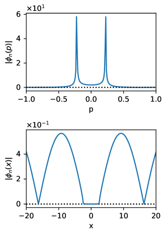
Figure 1: Example of an eigenfunction $\phi_{n}(p)$ obtained numerically by solving the integral equation (8). (a) Absolute value of $\phi_{n}(p)$. (b) Absolute value of the discrete Fourier transform of $\phi_{n}(p)$; in $x$-space the plateau centered at $x=0$ corresponds to the region where the potential is non-vanishing. The barrier parameters are $L=5$ and $V_{0}=20$ and $\phi_{n}(p)$ corresponds to the eigenvalue $\epsilon_{n}\approx 1.02$ (in natural units: $\hbar=1,c=1,\lambda=\hbar/mc=1$).

III.2 Numerical results

We now show typical numerical results for an initial wavepacket of the form

$$\psi_{f}(0,x)=(\theta(x-x_{0}+\Delta_{x}/2)-\theta(x-x_{0}-\Delta_{x}/2))\cos^{8}\left[\frac{\pi}{\Delta_{x}}\left(x-x_{0}\right)\right]e^{ip_{0}x},$$ (12)

corresponding to a wavefunction with mean position $x_{0}$ and momentum $p_{0}$ defined over the compact support $[x_{0}-\Delta_{x}/2,x_{0}+\Delta_{x}/2]$. The form $\cos^{8}$ is chosen to reduce the range in momentum space over which the Fourier transform takes significant values and hence simplify the resources needed for the numerical computations. Having solved Eq. (8) with the potential $V_{s}(x,\alpha)$, we use a fast Fourier transform on Eq. (7) to obtain the time-dependent wavepacket $\psi(t,x).$

The dynamics of a typical wavepacket for a small value of $\Delta_{x}$ (of the order of the Compton wavelength) is shown in Fig. 2. Part of the initial wavepacket [Fig. 2(a)] moves toward the left (corresponding to negative momenta components) while the other part scatters on the barrier, giving rise to a reflected and a small transmitted component (Fig. 2(b); beware of the different scale employed on the panels featuring the transmitted wavepacket). A small fraction of the transmitted component can be seen to move outside the light cone in Fig. 2(b) and (c).

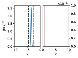
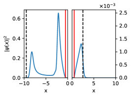
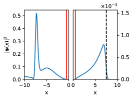
Figure 2: Probability density evolution of a wavepacket at $t=0$ (a), $t=5$ (b) and $t=10$ (c) in natural units (as defined in Fig. 1). The initial wavepacket is given by Eq. (12) with $x_{0}=-3.5,p_{0}=1$ and $\Delta_{x}=2$. The potential barrier depicted in red is given by Eq. (11) with $V_{0}=20,$ $L=1$ and $\alpha=20$. The dashed lines in (a) indicate the bounds of the compact support of the initial wavepacket; in (b) and (c), the dashed lines indicate the position of the light cone emanating from these bounds.

Fig. 3 focuses on the structure of the transmitted wavepacket right after exiting the barrier, as compared to the same initial wavepacket evolved freely. It can be seen that in both cases, part of the amplitude lies outside the light-cone, but the tunneled wavepacket displays a structure that is absent in the free case. This pattern varies with $L$. We will further analyze outside-the-light-cone propagation and compare it to the case of free propagation below (Sec. IV), as well as the properties of the transmitted peak as a function of the barrier and wavepacket parameters.

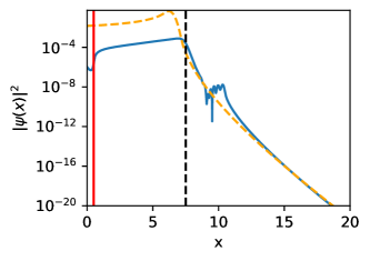
Figure 3: Probability density in logarithmic scale of the transmitted wave packet (blue line) at time $t=10$ (natural units) compared to the freely evolved wavepacket (yellow dashed line). In both cases, a fraction of the probability density lies beyond the light cone (dashed vertical line). The parameters of the initial wavepackets and the potential are the same as defined in Fig. 2.

III.3 The narrow potential case ($L\rightarrow 0$)

Let us now take the rectangular potential $V_{R}(x)$ of Eq. (10) and assume the width $L$ is small. To first order in $L,$ the eigenvalue equation (6) becomes

$$\epsilon_{n}\phi_{n}(p)=\sqrt{p^{2}c^{2}+m^{2}c^{4}}\phi_{n}(p)+\frac{V_{0}L}{2\pi}\int dp^{\prime}\phi_{n}(p^{\prime}).$$ (13)

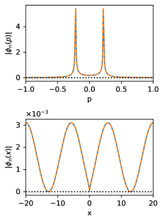
Figure 4: Modulus of the amplitude associated with an eigenfunction $\phi_{n}(p)$ with eigenvalue $\epsilon_{n}\approx 1.02$ in natural units (as defined in Fig. 1), in $p$-space (a) and $x$-space (b) for a potential of very small width $L\approx 0.08$ (corresponding to the discretization step in $x$) and $V_{0}L=1$. The analytical result given by Eq. (14) (yellow dashed lines) is computed on the same discretized points as the numerical solution (blue).

This is identical to the integral equation for the Salpeter equation in the presence of a Dirac $\delta$ potential at $x=0$. Such equations have been recently investigated [10, 11, 12], in particular in connection to bound states in an attractive Dirac potential. Setting the integral $I_{n}=\int dp^{\prime}\phi_{n}(p^{\prime})$ to be an unknown constant, Eq. (13) leads to

$$\phi_{n}(p)=\frac{1}{\epsilon_{n}-\sqrt{p^{2}c^{2}+m^{2}c^{4}}}\frac{V_{0}LI_{n}}{2\pi}.$$ (14)

Note that attempting to integrate this equation in order to obtain $I_{n}$ leads to a divergent integral. It was suggested [10] to renormalize the integral by employing dimensional regularization. Here the knowledge of the energy dependence of $I_{n}$ would be needed in order to integrate Eq. (7) and determine the time-dependent solution $\psi(t,x)$ by Fourier transform. For a given value of $\epsilon_{n}$ however we can rescale $\phi_{n}(p)$ with a global factor in order to compare Eq. (14) to our numerical solutions. An example is given in Fig. 4, showing a good agreement. While we have found it impossible to obtain analytical solutions by integrating Eq. (7) and Fourier transforming it, we point out that the solutions in the case of small $L$ present are similar to the one for larger values of $L$ shown in Fig. 2, save for the absence of the plateau centered at $x=0$ in $\phi_{n}(x)$ that precisely characterizes the width of the barrier.

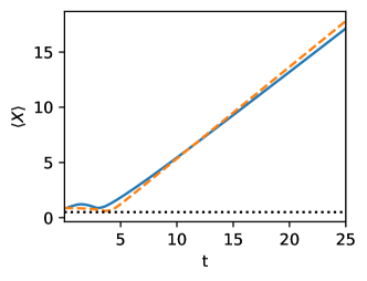
Figure 5: Mean value of the position of the transmitted wave packet for the tunneling case (blue line) and the free case (dashed yellow line). The parameters and units employed are the same as in Fig. 2.

IV Discussion

We have seen that broadly speaking tunneling in the relativistic Schrödinger equation appears to follows the familiar pattern known from non-relativistic tunneling [32, 33]. Most of the amplitude is reflected and only a wavepacket with a tiny amplitude is transmitted. One well-known feature of non-relativistic tunneling is that the average of the position of the transmitted peak is advanced, during a transient time interval, relative to the average position of the same wavepacket propagating freely. This is also the case here, as illustrated in Fig. 5. The evolution of the mean position of the transmitted wavepacket right after exiting the barrier, as a function of the barrier width or height, also follows the same pattern known for Schrödinger tunneling [33]. An example displaying the transmitted wavepacket as a function of the potential height is shown in Fig. 6.

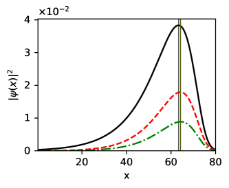
Figure 6: Transmited wavepackets at time $t=100$ in natural units (as defined in Fig. 1) for $V_{0}=2$ (red dashed line), $V_{0}=3$ (green dashed line) and the free case $V_{0}=0$ (black line). The initial wave packet is defined in Eq. (12) with $x_{0}=-22.25,p_{0}=1$ and $\Delta_{x}=20$. The colored vertical lines correspond to the $x$ value at which the corresponding packet is maximal.

As mentioned above, a specific feature of Salpeter wavepackets is their propagation outside the light-cone [16, 20, 21]. The fraction of the wavepacket propagating outside the light-cone (OLC) was quantified previously for free wavepackets [18]. It is interesting to look at the effect of the barrier on this type of propagation. An illustration is provided in Fig. 7, that shows the time-dependence of the OLC fraction of the right edge of the wavepacket in a typical situation. In the free case, OLC propagation appears as a transient effect that reaches a maximum at short times and then falls off gradually. In the tunneling case, the OLC fraction evolves at first like the one for the free wavepacket (essentially as the wavepacket is traveling toward the barrier) but an additional structure appears in the form of a second peak (or a plateau, depending on $L$). We hypothesize that this additional structure might result from superluminal waves of the first peak reflecting inside the barrier and then transmitted before being caught up by the light cone. This is supported by the fact that for larger barrier widths, the second structure disappears. Hence tunneling appears to have an effect on the OLC fraction only for small barrier widths.

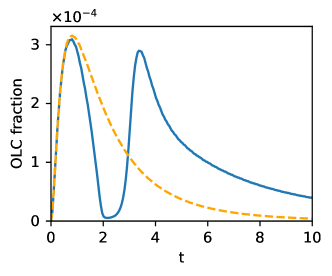
Figure 7: Outside the Light-Cone (OLC) fraction of the wavepacket (blue line) compared to the free case (dashed yellow line) as a function of time. At short times the behavior is similar, but in the tunneling case a second peak in the OLC fraction appears, whose form and amplitude depend on $L$ (here we have taken the same parameters and units as in Fig. 2).

We have also determined the behavior of the maximum value of the OLC fraction (irrespective of the time at which this maximum takes place) as a function of $V_{0}$ for different widths $L$. Results for a given initial wavepacket (identical in all cases considered) are displayed in Fig. 8. This figure quantifies the relative importance of the second OLC peak shown in Fig. 7, due to the presence of barrier, relative to the first peak, already present in free propagation (the free case OLC is visible in Fig. 8 by looking at the $V_{0}\rightarrow 0$ limit). The effect of the barrier on the OLC fraction of the transmitted wavepacket is only substantial for small values of $L$ (for $L=10$ natural units, the OLC fraction is seen to be identical to the one for free propagation) and for “moderate” values of $V_{0}$. This is consistent with the idea that the OLC structure due to tunneling is due to reflected waves (that are caught up by the light cone for larger values of $L$), although it does not explain the fact that for a given small value of $L$, there is an value of $V_{0}$ maximizing the OLC fraction (understandably, for large values of $V_{0}$, the reflected waves are too small to contribute to the OLC fraction significantly).

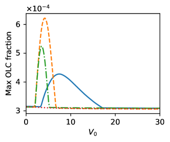
Figure 8: Global maximum value of the outside the light cone (OLC) fraction of the transmitted wavepacket as a function of $V_{0}$ for different barrier widths: $L=1$ (blue line), $L=2$ (orange dashed line), $L=2.5$ (green dashed line) and $L=10$ (red dotted line), for the same initial wavepacket having parameters $x_{0}=-(L/2+3)$, $p_{0}=1,$ $\Delta_{x}=2$. Numbers are given in natural units $c=\hbar=1,$ $\lambda=\hbar/mc=1$.

V Conclusions

We have investigated the tunneling dynamics for a particle scattering on a potential barrier in the context of the relativistic Schrödinger equation. While in the non-relativistic case or for standard relativistic equations potential tunneling can be handled approximately or asymptotically with plane-waves, the fact that the Salpeter equation contains a square-root operator renders the equation difficult to handle analytically beyond the free case [13, 3]. We have therefore undertaken a numerical approach by computing the solutions of the corresponding integral equation in momentum space.

The results indicate that the tunneling dynamics is similar to standard non-relativistic tunneling, or for that matter to the tunneling process for relativistic equations when the potential is far below the supercriticial threshold (as expected, the Salpeter equation does not display Klein tunneling in that case). The peculiar outside-the-light-cone propagation of the relativistic Schrödinger wavepackets was seen to be modified by the tunneling process only in the case of rather narrow barriers, the overall effect remaining however very small. It would be useful to develop analytical methods giving approximate transmission amplitudes as a function of the barrier parameters.

References

- [1] F. Lucha and F. F. Schoberl, Int. J. Mod. Phys. A 14(1999) 2309.
- [2] Rosenstein, B.; Horwitz, L.P. Probability current versus charge current of a relativistic particle. J. Phys. A Math. Gen. 1985, 18, 2115.
- [3] Kowalski, K.; Rembielinski, J. Salpeter equation and probability current in the relativistic Hamiltonian quantum mechanics. Phys. Rev. A 2011, 84, 012108.
- [4] A. Lattanzi. How to Deal with Nonlocality and Pseudodifferential Operators. An Example: The Salpeter Equation. In: Paranjape, M.B., MacKenzie, R., Thomova, Z., Winternitz, P., Witczak-Krempa, W. (Eds) Quantum Theory and Symmetries. CRM Series in Mathematical Physics (Springer, Cham, 2021).
- [5] Theodore J. Allen and M. G. Olsson, Reduction of the QCD string to a time component vector potential, Phys. Rev. D 68, 054022 (2003).
- [6] F. Buisseret and V. Mathieu, Hybrid mesons with auxiliary fields, Eur. Phys. J. A 29, 343–351 (2006).
- [7] I .J. Nickisch, L. Durand and B. Durand, Salpeter equation in position space: Numerical solution for arbitrary confining potentials, Phys. Rev. D 30, 660 (1984).
- [8] Richard L Hall, Wolfgang Lucha and Franz F Schoberl, Energy bounds for the spinless Salpeter equation: harmonic oscillator, J. Phys. A: Math. Gen. 34 (2001) 5059.
- [9] Y Chargui, L Chetouani and A Trabelsi, Analytical treatment of the one-dimensional Coulomb problem for the spinless Salpeter equation, J. Phys. A: Math. Theor. 42 (2009) 355203.
- [10] M. H. Al-Hashimi, A. M. Shalaby, and U.-J. Wiese, Asymptotic freedom, dimensional transmutation, and an infrared conformal fixed point for the -function potential in one-dimensional relativistic quantum mechanics, Phys. Rev. D 89, 125023 (2014).
- [11] Sergio Albeverio, Silvestro Fassari and Fabio Rinaldi, The discrete spectrum of the spinless one-dimensional Salpeter Hamiltonian perturbed by -interactions, J. Phys. A: Math. Theor. 48 185301 (2015).
- [12] Fatih Erman, Manuel Gadella, and Haydar Uncu, One-dimensional semirelativistic Hamiltonian with multiple Dirac delta potentials, Phys. Rev. D 95, 045004 (2017).
- [13] Rosenstein, B.; Usher, M. Explicit illustration of causality violation: Noncausal relativistic wave-packet evolution. Phys. Rev. D 1987, 36, 2381.
- [14] Al-Hashimi, M.H.; Wiese, U.J. Minimal position-velocity uncertainty wave packets in relativistic and non-relativistic quantum mechanics. Ann. Phys. 2009, 324, 2599–2621.
- [15] Eckstein, M.; Miller, T. Causal evolution of wave packets. Phys. Rev. A 2017, 95, 032106.
- [16] Pavsic, M. Localized States in Quantum Field Theory. Adv. Appl. Clifford Algebras 2018, 28, 89.
- [17] Torre, A.; Lattanzi, A.; Levi, D. Time-Dependent Free-Particle Salpeter Equation: Numerical and Asymptotic Analysis in the Light of the Fundamental Solution. Ann. Der Phys. 2017, 529, 1600231.
- [18] X. Gutierrez de la Cal and A. Matzkin, Beyond the light-cone propagation of relativistic wavefunctions: numerical results, Dynamics 3, 60 (2023).
- [19] Pavsic, M. Manifestly covariant canonical quantization of the scalar field and particle localization. Mod. Phys. Lett. A 33, 1850114 2018.
- [20] Hegerfeldt, G.C. Instantaneous spreading and Einstein causality in quantum theory. Ann. Phys. (Leipzig) 1998, 7, 716-725.
- [21] Kosinski, P. Salpeter Equation and Causality. Prog. Theor. Phys. 2012, 128, 59–65.
- [22] Greiner, W. Field Quantization; Springer: Berlin, Germany, 1996.
- [23] Brau, F. Integral equation formulation of the spinless Salpeter equation, J. Math. Phys. 39, 2254 (1998).
- [24] Gerhard C. Hegerfeldt and Simon N. M. Ruijsenaars, Remarks on causality, localization, and spreading of wave packets, Phys. Rev. D 22, 377 (1980).
- [25] Guillaumin-Espana, E; Salas-Brito, AL; Romero, RPMY; Nunez-Yepez, HN , Simple quantum systems in the momentum representation, Revista Mexicana de Física 47, 1 (2000)̇. [arXiv:physics/0001030]
- [26] M. I. Samar and V. M. Tkachuk, Exactly solvable problems in the momentum space with a minimum uncertainty in position, J. Math. Phys. 57, 042102 (2016).
- [27] Alkhateeb, M.; Gutierrez de la Cal, X.; Pons, M.; Sokolovski, D.; Matzkin, A. Relativistic time-dependent quantum dynamics across supercritical barriers for Klein-Gordon and Dirac particles. Phys. Rev. A 2021, 103, 042203.
- [28] L. Gavassino and M. M. Disconzi, Subluminality of relativistic quantum tunneling, Phys. Rev. A 107, 032209 (2023).
- [29] Alkhateeb, M.; Gutierrez de la Cal, X.; Pons, M.; Sokolovski, D.; Matzkin, A Quantum field approach to relativistic wavepacket tunneling: a fully causal process, in preparation.
- [30] Gutiérrez de la Cal, X.; Alkhateeb, M.; Pons, M.; Matzkin, A.; Sokolovski, D. Klein paradox for bosons, wave packets and negative tunnelling times. Sci. Rep. 2020, 10, 19225.
- [31] Alkhateeb, M.; Gutierrez de la Cal, X.; Pons, M.; Sokolovski, D.; Matzkin, in preparation.
- [32] H. M. Krenzlin, J. Budczies and K. W. Kehr, Wave packet tunneling, Ann. Phys. (Leipzig) 7, 732 (1998).
- [33] K. Smith and G. Blaylock, Simulations in quantum tunneling, Am. J. Phys. 85 763 (2017).