Algebraic Billiards in the Fermat Hyperbola

Abstract.

Algebraic billiards in a plane curve of degree $d\geq 2$ is a rational correspondence on a surface. The dynamical degree is an algebraic analogue of entropy that measures intersection-theoretic complexity. We compute a lower bound on the dynamical degree of billiards in the generic algebraic curve of degree $d$ over any field of characteristic coprime to $2d$, complementing the upper bound of [Wei23]. To do this, we specialize to a highly symmetric curve that we call the Fermat hyperbola. Over $\mathbb{C}$, we construct an algebraically stable model for this billiard via an iterated blowup. Over general fields, we compute the growth of a particular big and nef divisor.

1. Introduction

The classical billiard map is a discrete-time dynamical system that models a point particle bouncing around inside a billiard table, a plane region $\Omega\subset\mathbb{R}^{2}$ with smooth boundary [Gut12, Tab05]. The phase space of the billiard map is a subset of the real surface $\partial\Omega\times S^{1}$. The first factor tracks the position of the ball upon first collision with the boundary $\partial\Omega$, and the second factor tracks the ball’s direction of movement. After each collision, the direction of the ball is reflected across the tangent line to $\Omega$ at the collision point.

In this article, we study algebraic billiards, an extension of real billiards to algebraically closed fields ${\mathbf{k}}$ of characteristic not equal to $2$ [Glu14, Wei23]. The role of the billiard table is played by a given smooth curve $C\subset\mathbb{P}^{2}_{\mathbf{k}}$ of degree $d\geq 2$. The role of the space of directions $S^{1}$ is played by the circle

$$D\colonequals\{Q_{0}^{2}+Q_{1}^{2}=Q_{2}^{2}\}\subset\mathbb{P}^{2}_{\mathbf{k}}.$$

The billiards correspondence is a rational correspondence, i.e. a multivalued rational map, denoted

$$b:C\times D\vdash C\times D.$$

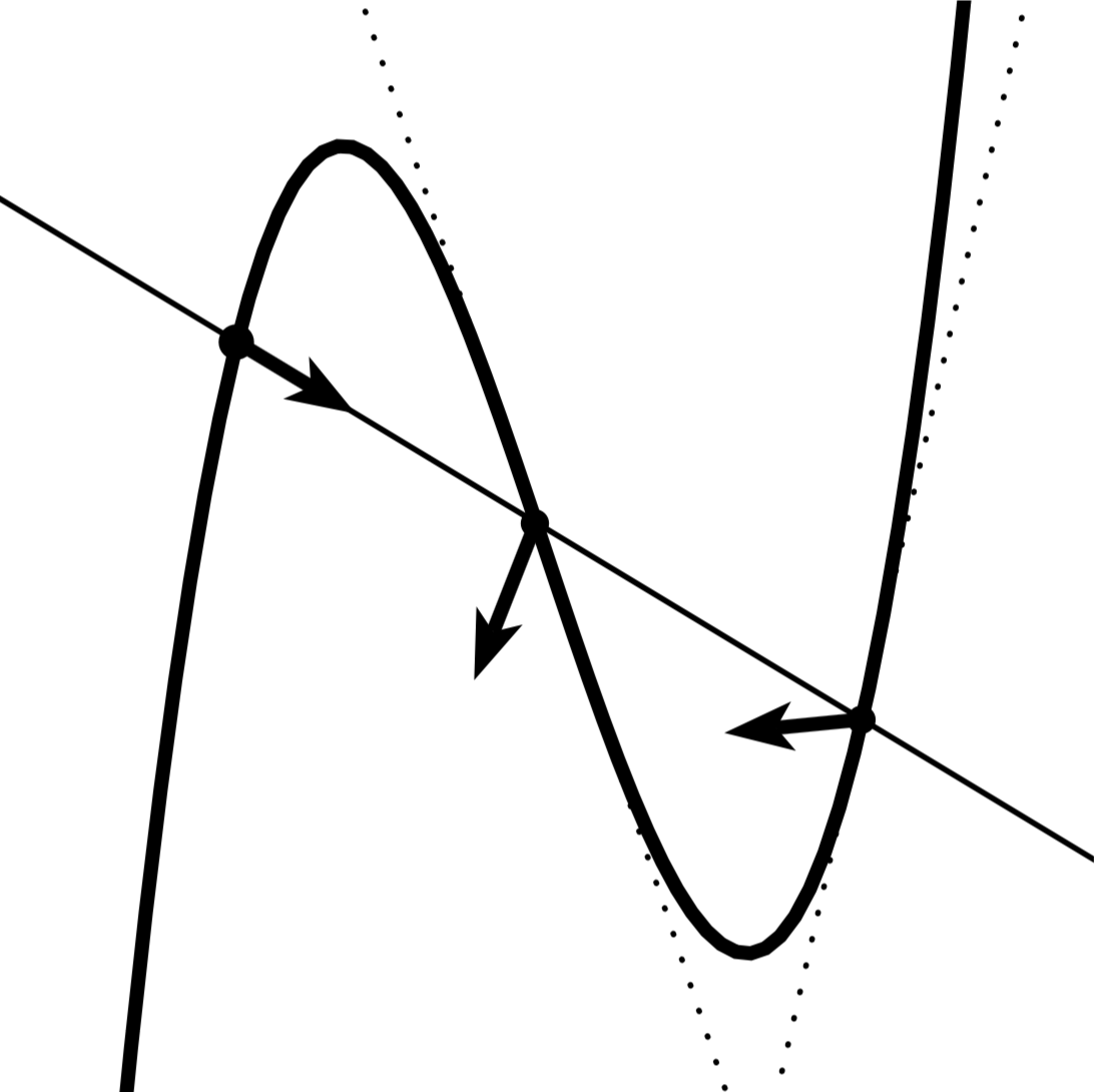
Figure 1. Algebraic billiards in the real curve defined by $x_{1}=x_{0}^{3}$. A generic input has two images.

For a general input $(x,v)\in C\times D$, the billiards image $b(x,v)$ is a set of $d-1$ points (Figure 1), obtained as follows. The line $\ell(x,v)$ through $x$ of direction $v$ is the line in $\mathbb{P}^{2}_{\mathbf{k}}$ through $x$ and $[Q_{0}:Q_{1}:0]$, if distinct. The secant correspondence $s$ is defined as

$$s:C\times D\vdash C\times D,$$

$$s(x,v)=\{(x^{\prime},v):x^{\prime}\in C\cap\ell(x,v)\smallsetminus c\}.$$

The reflection map

$$r:C\times D\dashrightarrow C\times D$$

is a birational involution $r(x,v)=(x,r_{x}(v))$, which we view as a rational family of involutions $r_{x}:D\to D$ over $C$. The map $r_{x}$ is reflection across the tangent line to $C$ at $x$ with respect to the quadratic form associated to $D$; see Section 3.1. Then billiards is defined by

$$b\colonequals r\circ s.$$

Topological and metric entropy of classical billiards is a well-studied and delicate subject [Mar18, Kat87, MZ21, ČT22, KSLP86, Che10]. We study the dynamical degree, an algebraic analogue of entropy.

Definition 1.1 ([DS08, Tru20]).

Let $X$ be a smooth projective surface equipped with a dominant rational correspondence $f:X\vdash X$. Each iterate $f^{n}$ induces a pushforward homomorphism $(f^{n})_{*}:\operatorname{Num}X\to\operatorname{Num}X$ on the group of divisor classes on $X$ modulo numerical equivalence. Choosing any ample class $\Delta$ in $\operatorname{Num}X$, the (first) dynamical degree is the limit

$$\lambda_{1}(f)\colonequals\lim_{n\to\infty}((f^{n})_{*}\Delta\cdot\Delta)^{1/n}.$$

This limit exists, is independent of $\Delta$, and is a birational conjugacy invariant. The algebraic entropy of $f$ is

$$h_{\operatorname{alg}}(f)\colonequals\log\lambda_{1}(f).$$

Dynamical degrees are very difficult to compute in general, even for rational maps. The only complete computations of $\lambda_{1}(f)$ for correspondences are for monomial correspondences and Hurwitz correspondences [DR21, Ram20].

In [Wei23], we proved an upper bound on the dynamical degree $\lambda_{1}$ of algebraic billiards in a smooth curve. In this article, we treat the more difficult problem of finding a lower bound on $\lambda_{1}$.

To do this, we identify a special curve in each degree, the Fermat hyperbola $C$, for which the dynamical degree can be computed on the nose. Then, by semicontinuity, we obtain a lower bound for very general curves $C_{\operatorname{gen}}$. Very general here means that $C_{\operatorname{gen}}$ admits an affine equation with algebraically independent parameters.

Theorem 1.2.

Fix $d\geq 2$, and let ${\mathbf{k}}$ be an algebraically closed field such that $\gcd(\operatorname{char}{\mathbf{k}},2d)=1$. Let $C\subseteq\mathbb{P}^{2}_{\mathbf{k}}$ be the Fermat hyperbola

$$C:\;(X_{0}-iX_{1})^{d}+(X_{0}+iX_{1})^{d}=X^{d}_{2}.$$

Let $D\subseteq\mathbb{P}^{2}_{\mathbf{k}}$ be the conic

$$D:\;Q_{0}^{2}+Q_{1}^{2}=Q_{2}^{2}.$$

The dynamical degree of the billiards correspondence $b:C\times D\vdash C\times D$ is

$$\lambda_{1}(b)=\psi_{d}\colonequals\frac{2d^{2}-3d+\sqrt{(2d^{2}-3d)^{2}-4(d-1)}}{2}.$$

Corollary 1.3.

Let $C_{\operatorname{gen}}\subset\mathbb{P}^{2}_{\mathbf{k}}$ be a very general curve of degree $d\geq 2$. Then the dynamical degree of the billiards correspondence $b_{\operatorname{gen}}:C_{\operatorname{gen}}\times D\vdash C_{\operatorname{gen}}\times D$ satisfies

$$\lambda_{1}(b_{\operatorname{gen}})\geq\frac{2d^{2}-3d+\sqrt{(2d^{2}-3d)^{2}-4(d-1)}}{2}\geq 2d^{2}-3d-1.$$

Combining this result with the upper bound $\rho_{d}$ obtained in our earlier work [Wei23] gives

$$2d^{2}-3d-1\leq\psi_{d}\leq\lambda_{1}(b_{\operatorname{gen}})\leq\rho_{d}<2d^{2}-d-3.$$

A heuristic complex-analytic argument suggests that $\lambda_{1}(b_{\operatorname{gen}})=\rho_{d}$ over $\mathbb{C}$ [WMdlP], but it is unclear whether this equality should hold over other fields. One of the main purposes of this article is therefore to prove lower bounds that apply in finite characteristic.

The Fermat hyperbola $C$ is the image of the standard Fermat curve, determined by the affine equation $x^{d}+y^{d}=1$, by a change of coordinates that takes $x^{2}+y^{2}=1$ to $x^{2}-y^{2}=1$. Its real locus resembles a dihedrally symmetric version of a hyperbola (Figure 2).

A correspondence $f\colon X\vdash X$ is algebraically stable if, for all $n\in\mathbb{N}$, the pushforward homomorphism $(f^{n})_{*}:\operatorname{Num}X\to\operatorname{Num}X$ satisfies $(f^{n})_{*}=(f_{*})^{n}$. If $f$ is not algebraically stable, computing $\lambda_{1}(f)$ may be difficult; such is the case with billiards. One typically seeks to get around this by constructing an algebraically stable model, a birational model of the domain on which the conjugate of $f$ is algebraically stable [FJ11, DF01]. Even for maps, such models may be difficult to construct, if they exist at all [Bir22]. We construct such a model for complex billiards in the Fermat hyperbola.

Theorem 1.4.

Over $\mathbb{C}$, the billiards correspondence in the Fermat hyperbola of degree $d\geq 2$ admits an algebraically stable model.

If $d=2$ or $d=3$, then $b$ can even be regularized (Proposition 5.6). Note that the Fermat hyperbola of degree $2$ is just the standard hyperbola $x^{2}-y^{2}=1$. The billiard correspondence in the hyperbola is a completely integrable birational map, conjugate to a translation map on an elliptic surface [Wei23, Corollary 7.11].

The dynamical degree $\lambda_{1}(b)$ only tracks the main term of the growth rate of $(b^{n})_{*}$. Theorem 1.4 is stronger in that it allows us to compute $(b^{n})_{*}$ exactly for all $n$, so in principle we could use it to prove Theorem 1.2 over $\mathbb{C}$. However, the archimedean distance on $\mathbb{C}$ is key to our proof of Theorem 1.4, whereas Theorem 1.2 holds in most characteristics. To prove Theorem 1.2, we construct what we call an essentially stable model. See Section 1.2.

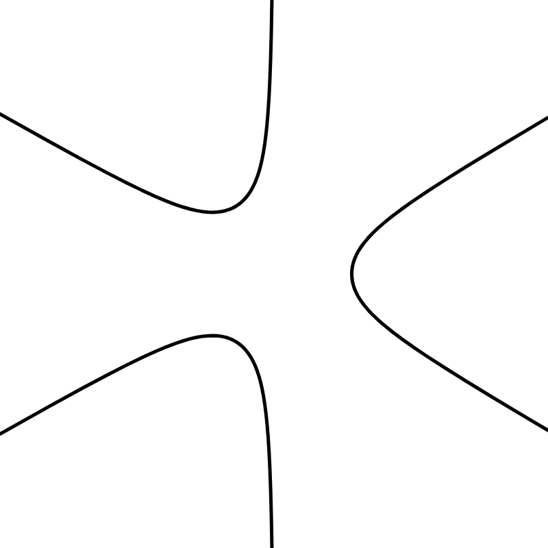
Figure 2. The real locus of the Fermat hyperbola of degree $d=3$, which is defined by the affine equation $2x_{0}^{3}-6x_{0}x_{1}^{2}=1$.

1.1. Related questions

To contextualize our work, we recall the Birkhoff Conjecture, a long-standing open problem in billiards. Chaos in a dynamical system is measured by topological entropy $h_{\operatorname{top}}\geq 0$. In classical billiards, the Birkhoff Conjecture predicts that the ellipse is the unique strictly convex, smooth curve $\partial\Omega$ for which $h_{\operatorname{top}}=0$; see [Gut12]. Yet it seems profoundly difficult to calculate $h_{\operatorname{top}}$, or even just show that $h_{\operatorname{top}}>0$, for any particular non-elliptical table. In this sense, we are far from understanding even the coarsest dynamical invariant of a “generic” billiard. Corollary 1.3 bounds the algebraic entropy $h_{\operatorname{alg}}(b)=\log\lambda_{1}(b)$ rather than $h_{\operatorname{top}}$, but the spirit is the same – to show that a typical algebraic billiard is chaotic unless $d=2$.

By [DS08], dynamical degrees control complex topological entropy from above. Specifically, one can show that:

1. If $b$ is the billiards correspondence in the Fermat hyperbola of degree $d\geq 2$, then the Dinh-Sibony topological entropy over $\mathbb{C}$ and Bowen-Dinaburg entropy over $\mathbb{R}$ are at most $\log\lambda_{1}(b)$.

2. The Bowen-Dinaburg topological entropy of the Lorentzian billiard ([KT09]) in the Fermat curve of degree $d$ is at most $\log\lambda_{1}(b)$. Indeed, the complexification of this system is isomorphic to $b$.

We omit the proofs, as they are very similar to [Wei23, Corollary 1.9].

One can also set up algebraic billiards so that the space of directions is $\mathbb{P}^{1}$, not $D$. Theorem 1.2 and Theorem 1.4 also hold in that context, thanks to a $2$-to-$1$ semiconjugacy [Wei23].

The Polynomial Birkhoff Conjecture for complex billiards, concerning the existence of polynomial first integrals, was recently proved by Glutsyuk [Glu21].

On the algebraic dynamics side, our work follows a substantial literature dedicated to constructing regular or algebraically stable models, particularly for rational maps of surfaces [DF01, FJ11, Bir22]. Birational surface maps admit algebraically stable models, and their dynamical degrees are quadratic integers [DF01]. On the other hand, there are rational but not birational maps of $\mathbb{P}^{2}$ with no algebraically stable model [Fav03, BDJ20]. No general results on constructing improved models for surface correspondences are yet known.

1.2. Proof sketch

In [Wei23], we introduced a modified phase space, i.e. a birational model, on which the degree growth of billiards in curves is easier to control. Let $C_{\operatorname{gen}}$ be a very general curve and let $b_{\operatorname{gen}}=r_{\operatorname{gen}}\circ s_{\operatorname{gen}}$ be its billiard correspondence. The modified phase space is $P_{\operatorname{gen}}\to C_{\operatorname{gen}}\times D$, the simple blowup of $C_{\operatorname{gen}}\times D$ at $\operatorname{Ind}s_{\operatorname{gen}}\cup\operatorname{Ind}r_{\operatorname{gen}}$. The model $P_{\operatorname{gen}}$ is conjecturally algebraically stable [Wei23].

In this work, our strategy is to produce a kind of degeneration $P\to C\times D$ of $P_{\operatorname{gen}}\to C_{\operatorname{gen}}\times D$ suited to the Fermat hyperbola $C$. The idea is as follows. A key property of $P_{\operatorname{gen}}$ is that it regularizes the reflection map $r_{\operatorname{gen}}:C_{\operatorname{gen}}\times D\dashrightarrow C_{\operatorname{gen}}\times D$. That is, the conjugate of $r_{\operatorname{gen}}$ to $P_{\operatorname{gen}}$ is a biregular correspondence. But in the case of the Fermat hyperbola, a simple blowup above $\operatorname{Ind}r$ is insufficient to regularize $r$ because the isotropic scratch points are non-basic, being flexes of $C$. Our “modified phase space” for $C\times D$ should at least regularize $r$.

We therefore define a blowup

$$\pi:P\to C\times D$$

that is a simple blowup over $\operatorname{Ind}s$ and a $(d-1)$-fold iterated blowup over $\operatorname{Ind}r$, chosen to regularize $r$. As $C_{\operatorname{gen}}$ approaches $C$, groups of $d$ basic isotropic scratch points of $C_{\operatorname{gen}}$ degenerate to non-basic isotropic scratch points of $C$. It is conceptually convenient to think of $P$ as a degeneration of $P_{\operatorname{gen}}$ in which some blowup centers have come together.

Because the points of $\operatorname{Ind}r$ are flexes of $C$, understanding $s$ on the blowup above $\operatorname{Ind}r$ becomes a local matter. Hence it is actually easier to work with $P$ than with $P_{\operatorname{gen}}$. This observation is the crucial point that distinguishes $C$ in the family $C_{\operatorname{gen}}$.

If ${\mathbf{k}}=\mathbb{C}$, the model $P$ is algebraically stable if and only if $d=2$ or $d$ is odd. Algebraic stability is proved by observing that the forward orbits of contracted curves are not Zariski dense in $P$, reducing the problem to elementary $1$-dimensional complex dynamics. A minor modification $P_{+}$ of the construction produces an algebraically stable model over $\mathbb{C}$ if $d>2$ is even.

Over other base fields ${\mathbf{k}}$, the model $P$ may fail to be algebraically stable regardless of parity of $d$, for instance if $2d-1=0$ in ${\mathbf{k}}$. Nevertheless, we show that $P$ is essentially stable, a new definition. That is, there exists a big and nef divisor $\Delta$ on $P$ for which the conjugate $\hat{b}:P\vdash P$ of $b$ satisfies

$$(\hat{b}^{n})_{*}\Delta\cdot\Delta=(\hat{b}_{*})^{n}\Delta\cdot\Delta.$$

This allows us to compute $\lambda_{1}(\hat{b})$, even in the absence of algebraic stability.

Outline

The reader will be greatly aided by first looking over Sections 1-6 of [Wei23]; we use results from Sections 3, 4, and 6. The contents of this paper are as follows.

Section 2: mostly standard background on correspondences and dynamical degrees.

Section 3: we recall the foundations of algebraic billiards, introduce the Fermat hyperbola, and construct useful birational models $P$ and $P_{+}$ of $C\times D$.

Section 4: We show that $P$ and $P_{+}$ are regular models for $r$.

Section 5: We compute the contracted curves and indeterminacy of the conjugates of $s$ and $r$ to $P$ and $P_{+}$, and we compute their actions on exceptional divisors.

Section 6: We show that billiards is essentially stable on $P$ and prove Theorem 1.2 ($=$ Theorem 6.7).

Section 7: We analyze algebraic stability when ${\mathbf{k}}=\mathbb{C}$, proving Theorem 1.4 ($=$ Theorem 7.1).

Acknowledgments

We thank Richard Birkett, Laura DeMarco, Jeff Diller, and Alexey Glutsyuk for helpful conversations related to this work. Thanks to Anna Dietrich for invaluable assistance preparing the manuscript. The diagrams were prepared with Desmos and GeoGebra. This material is based upon work supported by the National Science Foundation under Award No. 2202752.

2. Preliminaries

This section contains background on correspondences over an algebraically closed field ${\mathbf{k}}$. The facts are mostly well-known, but we have to introduce some nonstandard terminology (i.e. contracted curve vs. contraction). Background on divisors and intersection theory may be found in [Ful98, EH16].

All surfaces are smooth, projective, and irreducible.

2.1. Correspondences

Definition 2.1.

Given irreducible projective varieties $X$ and $Y$ of the same dimension, a rational correspondence $f=(\Gamma_{f},X,Y)$, also written $f:X\vdash Y$, is an effective algebraic cycle in $X\times Y$ of the form

$$\Gamma_{f}=\sum_{i=1}^{\nu}m_{i}[\Gamma_{i}]\neq 0,$$

such that each summand satisfies $\dim\Gamma_{i}=\dim X$. We have projection maps

$$\Pi_{1}:X\times Y\to X,\quad\Pi_{2}:X\times Y\to Y.$$

Let

$$\pi_{1}:\Gamma_{f}\to X,\quad\pi_{2}:\Gamma_{f}\to Y$$

be the restrictions of $\Pi_{1},\Pi_{2}$ to the support of $\Gamma_{f}$.

A rational correspondence is dominant if the projections $\pi_{1},\pi_{2}$ restrict to dominant, generically finite morphisms on each component $\Gamma_{i}$. For the rest of the paper, all correspondences are dominant.

We may also write $f=(\Gamma_{f},\pi_{1},\pi_{2})$ when it is helpful to remember the projections.

Writing $m=\deg\pi_{2}$ and $n=\deg\pi_{1}$, we say that $f$ is an $m$-to-$n$ rational correspondence. We write

$$\deg_{1}f\colonequals\deg\pi_{1},\quad\deg_{2}f\colonequals\deg\pi_{2}.$$

The adjoint of $f:X\vdash Y$ is the correspondence $g:Y\vdash X$, defined by taking the image of $\Gamma_{f}$ in $Y\times X$ under $(x,y)\mapsto(y,x)$.

The rational correspondence $f$ is regular if the projection $\pi_{1}$ is finite, rather than just generically finite. Note that a $m$-to-$1$ regular dominant correspondence over $\mathbb{C}$ with a reduced graph is just a surjective holomorphic map $X\to Y$ of generic topological degree $m$.

The indeterminacy locus and exceptional locus are the varieties

$$\operatorname{Ind}f=\{x\in X:\pi_{1}^{-1}(x)\text{ is not finite}\},$$

$$\operatorname{Exc}f=\{y\in Y:\pi_{2}^{-1}(y)\text{ is not finite}\}.$$

We are interested only in curve and surface correspondences. Dominant curve correspondences are biregular.

The following terminology is helpful in the study of surface correspondences.

Definition 2.2.

Let $f:X\vdash Y$ be a dominant correspondence of smooth, irreducible projective surfaces.

A contraction of $f$ is an irreducible curve $V\subset\Gamma_{f}$ such that $\pi_{2}(V)$ is a point. A contracted curve is an irreducible curve $W\subset X$ such that $\pi_{1}^{-1}(W)$ contains a contraction.

An expansion of $f$ is an irreducible curve $V\subset\Gamma_{f}$ such that $\pi_{1}(V)$ is a point. An exceptional image curve is a irreducible curve $W\subset Y$ such that $\pi_{2}^{-1}(W)$ contains an expansion.

Definition 2.3.

Suppose that $W\subset X$, $W^{\prime}\subset Y$ are irreducible curves. The dominant restriction of $f$, denoted $f|_{W\vdash W^{\prime}}$, is the dominant curve correspondence $W\vdash W^{\prime}$ obtained from $\Gamma_{f}|_{W\times W^{\prime}}$ by removing any components on which either of the projections fails to be dominant. The dominant restriction is only defined if nonempty.

It is often useful to view correspondences as set-valued maps, as follows.

Definition 2.4.

The (total) image of a set $\Sigma\subset X$ by $f$ is

$$f(\Sigma)\colonequals\pi_{2}(\pi_{1}^{-1}(\Sigma)).$$

It is also useful to define a notion of image that avoids indeterminacy. The strict image of a set $\Sigma\subset X$ by $f$, denoted $f_{\operatorname{str}}(\Sigma)$, is the Zariski closure in $Y$ of $f(\Sigma\smallsetminus\operatorname{Ind}f)$.

Note that the image of a contracted curve can be 1-dimensional. The image of an indeterminacy point always includes at least one exceptional image curve.

The following lemma helps us compute images.

Lemma 2.5.

Let $f:X\vdash Y$ be an $m$-to-$n$ rational correspondence of smooth projective surfaces, and let $p\in X$. If $f(p)$ contains a set $\Sigma$ of isolated points of total multiplicity $n$, then $f(p)=\Sigma$.

Proof.

This is a consequence of Stein factorization applied to $\pi_{1}$ [Har13, III.11.5]. ∎

Definition 2.6.

We may form the composite

$$g\circ f:X\vdash Z$$

of a pair of dominant rational correspondences

$$f:X\vdash Y,\quad g:Y\vdash Z.$$

It is defined by its graph, as follows.

The total composite graph of $f$ and $g$ is the scheme-theoretic image of $\Gamma_{f}\times_{Y}\Gamma_{g}$ in $X\times Z$. It is a $2$-cycle. The graph $\Gamma_{g\circ f}$ is obtained by removing all components $\Gamma$ from the total composite graph on which either projection fails to be dominant.

One also sees the following equivalent construction. Let $V=Y\smallsetminus\operatorname{Ind}g$ and let $U=f^{-1}(V)\smallsetminus\operatorname{Ind}f$. Let $\pi:U\times V\times Z\to U\times Z$ be the projection forgetting the $V$ factor. Then define

$$\Gamma^{U\times Z}_{g\circ f}\colonequals\pi\left(\Gamma_{f}|_{U\times V}\times_{V}\Gamma_{g}|_{V\times Z}\right).$$

Then $\Gamma_{g\circ f}$ is defined as the Zariski closure of $\Gamma^{U\times Z}_{g\circ f}$ in $X\times Z$. We extend this definition linearly to $f$ and $g$ with graphs with non-reduced or multiple irreducible components.

2.2. Formal correspondences

Throughout this paper, it will be most convenient to do local calculations in power series. To justify this simplification, we outline a theory of formal regular and rational correspondences of smooth surface germs. This is an extension of the theory of holomorphic or meromorphic fixed point germs [FJ04, FJ07] to correspondences over arbitrary algebraically closed base fields. There are purely algebraic proofs over $\mathbb{C}$ that generalize without difficulty given the correct vocabulary. We therefore only give proofs for claims where there are differences between maps and correspondences.

For formal schemes, see [Har13, II.9]. In this paper, all formal schemes are obtained from projective schemes by completion and restriction to closed formal subschemes. Let $X$ be a projective surface, let $x\in X$ be a smooth point of $X$, and let $G$ be the formal neighborhood of $X$ at $x$. We think of $G$ as a germ. It is isomorphic to the one-point formal scheme $(\mathbb{A}^{2},0)$ that has structure sheaf ${\mathbf{k}}[[x_{0},x_{1}]]$ at $x$, see [Har13, II.9.3.4].

An iterated blowup $\pi:G_{\pi}\to G$ is the formal scheme morphism obtained by a composition of finitely many point blowups starting from $G$,

$$G_{\pi}=G_{\ell}\to\ldots\to G_{0}=G.$$

It is naturally isomorphic to the formal neighborhood of the exceptional divisor upon blowing up the ambient surface of $G$ via $\pi$.

The exceptional curves in $G_{\pi}$ are the exceptional image curves of $\pi^{-1}$. They generate a free abelian group $\operatorname{Div}G_{\pi}$. Iterated blowups form an inverse system for the relation of domination, defined by

$$\pi^{\prime}\trianglerighteq\pi\quad\Leftrightarrow\quad\exists\;\tilde{\pi}\colon\pi^{\prime}=\pi\circ\tilde{\pi},$$

where $\tilde{\pi}$ is a composition of point blowups. If $G_{\pi}\neq G$, then the underlying scheme of $G_{\pi}$ is the union of the exceptional curves.

Let $G_{1},G_{2}$ be iterated blowups of $G$. A formal rational $m$-to-$n$ correspondence $f:G_{1}\vdash G_{2}$ is given by its graph $\Gamma_{f}\subset G_{1}\times G_{2}$, a formal effective $2$-cycle such that the two projections restricted to all sufficiently small infinitesimal neighborhoods approximating the scheme part of $G_{1}\times G_{2}$ are generically finite of degrees $\deg_{2}f=n$ and $\deg_{1}f=m$ respectively.

All such correspondences in this paper are obtained by restricting correspondences on varieties as defined in Section 2.1.

Given exceptional curves $W\subset G_{\pi}$, $W^{\prime}\subset G_{\pi^{\prime}}$, we may define the dominant restriction $f|_{W\vdash W^{\prime}}$ if nonempty.

Lemma 2.7.

Say $f:G_{\pi}\vdash G_{\pi^{\prime}}$. Then there exists $\pi^{\prime\prime}\trianglerighteq\pi^{\prime}$ such that

$$f_{\pi\pi^{\prime\prime}}\colonequals(\pi^{\prime\prime})^{-1}\circ\pi^{\prime}\circ f$$

has no contracted curves.

Proof.

There exist finitely many contractions of $\tau:\tilde{\Gamma}_{f}\to G_{\pi^{\prime}}$, where $\tilde{\Gamma}_{f}$ is the desingularized graph of $f$. Call this number $\nu(f)$. Let $p\in G_{\pi^{\prime}}$ be the image of a contraction of $\tau$. Let $\pi_{0}^{\prime}\trianglerighteq\pi^{\prime}$ be obtained by $\pi^{\prime}_{0}=\pi^{\prime}\circ\pi_{p}$, where $\pi_{p}$ is the blowup at $p$. Let $E_{p}=\pi_{p}^{-1}(p)$. Then, by the universal property of blowing up, at least one contracted curve of $\tau$ is mapped onto $E_{p}$ by $\pi_{p}^{-1}\circ\tau$. Continuing in this fashion, after at most $\nu(f)$ point blowups, we obtain $\pi^{\prime\prime}\trianglerighteq\ldots\trianglerighteq\pi^{\prime}_{0}\trianglerighteq\pi^{\prime}$ such that the map $\tilde{\Gamma}_{f_{\pi\pi^{\prime\prime}}}\to G_{\pi^{\prime\prime}}$ has no contracted curves. Hence, neither does $\Gamma_{f_{\pi\pi^{\prime\prime}}}\to G_{\pi^{\prime\prime}}$. ∎

Remark 2.8.

We cannot necessarily find $\pi^{\prime\prime}\trianglerighteq\pi$ and $\pi^{\prime\prime\prime}\trianglerighteq\pi^{\prime}$ such that $f_{\pi^{\prime\prime}\pi^{\prime\prime\prime}}$ is both contraction-free and indeterminacy-free, unlike the case of rational maps.

Lemma 2.9 (Contracted curve test).

Say $f:G_{\pi}\vdash G_{\pi^{\prime}}$. Suppose that $\Delta$ is a prime divisor on $G_{\pi}$ such that

$$\sum_{\Delta^{\prime}}\deg_{1}f|_{\Delta\vdash\Delta^{\prime}}=\deg_{1}f,$$

where $\Delta^{\prime}$ ranges over curves in $f(\Delta)$. Then $\Delta$ is not a contracted curve of $f$.

Proof.

We prove the contrapositive. Let $f=(\Gamma_{f},\tau_{1},\tau_{2})$. Say $\Delta\times p$ is a contraction. By Lemma 2.7, there exists $\pi^{\prime\prime}\trianglerighteq\pi^{\prime}$ such that $f_{\pi\pi^{\prime\prime}}$ has no contractions, so the projection $\Gamma_{f_{\pi\pi^{\prime\prime}}}$ to $X_{\pi^{\prime\prime}}$ is finite. Let $\pi^{\prime\prime}=\pi^{\prime}\circ\tilde{\pi}$. Let $\bigcup_{i=1}^{\ell}\Delta^{\prime\prime}_{i}$ be the strict image of $\Delta$ in $X_{\pi^{\prime\prime}}$. For each $i$, if $\tilde{\pi}(\Delta^{\prime\prime}_{i})$ is a curve, then

$$\deg_{1}f_{\pi\pi^{\prime}}|_{\Delta\vdash\tilde{\pi}(\Delta^{\prime\prime}_{i})}=\deg_{1}f_{\pi\pi^{\prime\prime}}|_{\Delta\vdash\Delta^{\prime\prime}}.$$

By the universal property of blowing up, the exceptional curve of the blowup at $p$ appears among the $\Delta^{\prime\prime}_{i}$. Therefore,

$$\sum_{\Delta^{\prime}}\deg_{1}f|_{\Delta\vdash\Delta^{\prime}}<\sum_{\Delta^{\prime\prime}_{i}}\deg_{1}f|_{\Delta\vdash\Delta^{\prime\prime}_{i}}=\deg_{1}f.$$

∎

2.3. Action on divisors

Let $f:X\vdash X$ be a dominant rational correspondence. Let $\operatorname{Div}X$ denote the group of Weil divisors on $X$. Let $\operatorname{DivCl}X$ be $\operatorname{Div}X$ modulo linear equivalence. Let $\operatorname{Num}X$ be $\operatorname{Div}X$ modulo numerical equivalence.

Definition 2.10.

There are induced pushforward homomorphisms

$$f_{*}:\operatorname{Div}X\to\operatorname{Div}X,\quad f_{*}:\operatorname{DivCl}X\to\operatorname{DivCl}X,\quad f_{*}:\operatorname{Num}X\to\operatorname{Num}X.$$

Let $u:V\to W$ be a generically finite and dominant morphism of smooth projective surfaces or formal surfaces, and let $\Delta$ be a prime divisor of $V$.

We define $u_{*}:\operatorname{Div}V\to\operatorname{Div}W$ as follows. If $u(\Delta)$ is a point, then we define $u_{*}\Delta=0$. Otherwise $u(\Delta)$ is a curve. Denote the generic point of $\Delta$ by $\eta$ and the generic point of $u(\Delta)$ by $\theta$. We define

$$u_{*}\Delta=[{\mathbf{k}}(\theta):{\mathbf{k}}(\eta)]u(\Delta).$$

We extend $u_{*}$ to all divisor classes by linearity. It descends to $u_{*}:\operatorname{DivCl}V\to\operatorname{DivCl}W$ and then to $u_{*}:\operatorname{Num}V\to\operatorname{Num}W$.

There are also pullback homomorphisms

$$u^{*}:\operatorname{Div}W\to\operatorname{Div}V,\quad u^{*}:\operatorname{DivCl}W\to\operatorname{DivCl}V,\quad u^{*}:\operatorname{Num}W\to\operatorname{Num}V.$$

Rather than present a full definition, we just explain how to compute these in our setting. Let $\Delta$ be a prime divisor of $W$. If $\deg u=d$ and the inverse image of a general point of $\Delta$ consists of $d$ distinct points, then

$$u^{*}\Delta=u^{-1}(\Delta).$$

If $f:X\vdash Y$, defined by $(\Gamma_{f},\pi_{1},\pi_{2})$, is a correspondence with a smooth and irreducible graph, then the pushforward homomorphism is

$$f_{*}:\operatorname{Num}X\to\operatorname{Num}Y,$$

$$f_{*}=(\pi_{2})_{*}\circ(\pi_{1})^{*}.$$

This definition may be extended to graphs $\Gamma_{f}$ with singular components by working instead on a desingularized graph. We recall a standard lemma that shows how to compute $f_{*}$ without desingularizing.

Lemma 2.11.

Let $f:X\vdash Y$ be a dominant correspondence of smooth, irreducible projective surfaces, let $\Delta\in\operatorname{Num}X$, and let $\Delta^{\prime}\in\operatorname{Num}Y$. Let $\Pi_{1}:X\times Y\to X$ and $\Pi_{2}:X\times Y\to Y$ be the projections. Let $\iota_{f}(\Delta,\Delta^{\prime})\colonequals f_{*}\Delta\cdot\Delta^{\prime}$. Then

(1) $$\iota_{f}(\Delta,\Delta^{\prime})=\Gamma_{f}\cdot\Pi_{1}^{*}\Delta\cdot\Pi_{2}^{*}\Delta^{\prime}.$$

Proof.

The proof given in [Roe15, Section 3] for rational maps over $\mathbb{C}$ adapts to our setting. ∎

Pullback and pushforward are functorial for regular correspondences, but not for rational correspondences in general. The following criterion, stemming from work of Diller-Favre, describes when pushforward interacts well with composition [DF01, Proposition 1.13].

Lemma 2.12.

Let $f:X\vdash Y$, $g:Y\vdash Z$ be dominant correspondences of smooth, irreducible projective surfaces. Let $f=(\Gamma_{f},\pi_{1},\pi_{2}).$ If, for every contraction $V$ of $f$, we have

$$\pi_{2}(V)\cap\operatorname{Ind}g=\varnothing,$$

then $(g\circ f)_{*}=g_{*}\circ f_{*}$.

Proof.

The proof given in [Roe15, Proposition 1.4] for rational maps over $\mathbb{C}$ adapts to our setting. ∎

Definition 2.13.

Let $f:X\vdash Y$. The strict transform of a prime divisor $\Delta\in\operatorname{Div}X$ is the divisor

$$f_{\operatorname{str}}\Delta\colonequals\sum_{V}m_{V}V,$$

where $V$ ranges over curves in the set $f_{\operatorname{str}}\Delta$ and $m_{V}$ is the weight of $V$ in $f_{*}\Delta$. We extend this linearly to a homomorphism $\operatorname{Div}X\to\operatorname{Div}Y$.

2.4. Dynamical degrees

We work in Truong’s framework.

Definition 2.14 ([Tru20]).

Let $f:X\vdash X$ be a rational correspondence on a smooth projective surface $X$ over ${\mathbf{k}}$. Let $f_{*}:\operatorname{Num}X\to\operatorname{Num}X$ be pushforward. Let $\Delta\in\operatorname{Num}X$ be an ample class. The (first) dynamical degree of $f$, denoted $\lambda_{1}(f)$, is the quantity

(2) $$\lambda_{1}(f)\colonequals\lim_{n\to\infty}((f^{n})_{*}\Delta\cdot\Delta)^{1/n}.$$

The limit (2) exists and is independent of the choice of $\Delta$.

Definition 2.15.

Let $f:X\vdash X$ be a rational correspondence on an irreducible projective smooth surface $X$. We say $f$ is algebraically stable if $(f_{*})^{n}=(f^{n})_{*}$ on $\operatorname{Num}X$ for all $n\in\mathbb{N}$.

Theorem 2.16.

Let $f:X\vdash X$, $f=(\Gamma_{f},\pi_{1},\pi_{2})$ be a dominant rational correspondence on an irreducible projective smooth surface $X$.

1. The dynamical degree $\lambda_{1}(f)$ is a birational conjugacy invariant of the pair $(X,f)$. That is, if $g:Y\dashrightarrow X$ is a birational map, then

   $$\lambda_{1}(f)=\lambda_{1}(g^{-1}\circ f\circ g).$$

2. If for all contractions $V$ of $f$ and all $n\in\mathbb{N}$, we have

   $$f^{n-1}(\pi_{2}(V))\cap\operatorname{Ind}f=\varnothing,$$

   then $f$ is algebraically stable.

3. Let $S$ be a smooth, integral scheme with generic point $\eta$. Let $\pi:X\to S$ be a projective, smooth, surjective morphism of relative dimension $2$. Let $X_{p}$ denote the fiber at $p\in S$. Let $f:X\vdash X$ be a rational correspondence over $S$ with the property that, for each $p\in S$, the restriction $\Gamma_{f}|_{X_{p}\times X_{p}}$ is the graph of a dominant rational correspondence $f_{p}:X_{p}\vdash X_{p}$. Then, for all $p\in S$, we have

   $$\lambda_{1}(f_{p})\leq\lambda_{1}(f_{\eta}).$$

Claim (1) is a deep theorem of Truong [Tru20, Theorem 1.1]. Claim (2) follows from iterating Lemma 2.12. Claim (3) is a straightforward generalization of [Xie15, Lemma 4.1]; see also [Wei23, Theorem 2.18 (5)].

3. Billiards and blowups

3.1. Setup

In this subsection, we recall the definition of the algebraic billiards correspondence, following [Wei23]. We limit attention to the case of smooth separable plane curves over a field ${\mathbf{k}}$ of characteristic not equal to $2$.

Let $X=\mathbb{P}^{2}$ with coordinates $[X_{0}:X_{1}:X_{2}]$, and $Q=\mathbb{P}^{2}$ with coordinates $[Q_{0}:Q_{1}:Q_{2}]$. We introduce affine coordinates

$$x_{0}=\frac{X_{0}}{X_{2}},\quad x_{1}=\frac{X_{1}}{X_{2}},\quad q_{0}=\frac{Q_{0}}{Q_{2}},\quad q_{1}=\frac{Q_{1}}{Q_{2}}.$$

These coordinates define the main affine subsets

$$\mathbb{A}^{2}=\operatorname{\text{Spec}}{\mathbf{k}}[x_{0},x_{1}]\subset X,\quad\mathbb{A}^{2}=\operatorname{\text{Spec}}{\mathbf{k}}[q_{0},q_{1}]\subset Q.$$

Having chosen these affines, there is a distinguished line at infinity in each of $X$ and $Q$.

Fix $d\geq 2$. Let $C\subset X$ be a smooth, irreducible curve of degree $d$, defined by some affine equation $f_{C}(x_{0},x_{1})=0$.

Define the curve $D\subset Q$ by

$$D:\;Q_{0}^{2}+Q_{1}^{2}=Q_{2}^{2}.$$

Points of $D$ are called directions. There is a $2$-to-$1$ ramified cover, the slope map, defined by

$$[\cdot]:D\to\mathbb{P}^{1},$$

$$[Q_{0}:Q_{1}:Q_{2}]\mapsto[Q_{0}:Q_{1}].$$

The points of $C$ and $D$ at infinity are just the points of $C$ and $D$ in $X\smallsetminus\mathbb{A}^{2}$ and $Q\smallsetminus\mathbb{A}^{2}$, respectively. We denote the sets of such points by

$$C_{\infty}\colonequals C\cap(X\smallsetminus\mathbb{A}^{2}),$$

$$D_{\infty}\colonequals D\cap(Q\smallsetminus\mathbb{A}^{2}).$$

The billiards correspondence $b$ associated to the curve $C$ is a rational correspondence

$$b:C\times D\vdash C\times D,$$

$$b=r\circ s,$$

where $s$ is secant and $r$ is reflection, defined as follows.

We need to give defining equations for $\Gamma_{s}$, $\Gamma_{r}$ in $(C\times D)^{2}$. We denote the first and second factors of this product by $C\times D$ and $C^{\prime}\times D^{\prime}$, respectively, and similarly add a prime to denote any quantity that is defined in the second factor.

We define a relation $S^{\operatorname{pre}}_{+}$ on $X\times Q$, via its graph, as the subvariety $X\times Q\times X^{\prime}\times Q^{\prime}$ cut out by the equations

(3) $$q=q^{\prime},$$

(4) $$\begin{vmatrix}X_{0}&X^{\prime}_{0}&Q_{0}\\ X_{1}&X^{\prime}_{1}&Q_{1}\\ X_{2}&X^{\prime}_{2}&0\end{vmatrix}=0.$$

Let $S_{+}$ be the variety obtained from $S_{+}^{\operatorname{pre}}$ by discarding all components with a non-dominant projection to $X\times Q$ or $X^{\prime}\times Q^{\prime}$. Restricting $S_{+}$ to $C\times D\times C^{\prime}\times D^{\prime}$ gives us a relation $s_{+}$ on $C\times D$. Notice that the graph $\Gamma_{s_{+}}$ contains the graph $\Gamma_{1}$ of the identity map. The secant correspondence

$$s:C\times D\vdash C\times D$$

is the relation with graph

$$\Gamma_{s}=\Gamma_{s_{+}}-\Gamma_{1}.$$

Then $s$ is in fact a dominant $(d-1)$-to-$(d-1)$ rational correspondence [Wei23, Proposition 3.7].

Reflection is defined as follows. Let $t:C\to\mathbb{P}^{1}$, $t(x)=[t(x)_{0}:t(x)_{1}]$ be the Gauss map; it sends $x\in C\smallsetminus C_{\infty}$ to

$$t(x)=\left[-\frac{\partial f_{c}}{\partial x_{1}}:\frac{\partial f_{c}}{\partial x_{0}}\right].$$

This is defined because $C$ was assumed separable. Let $R^{\operatorname{pre}}_{+}$ be the relation on $C\times Q$ defined by the equations

$$x=x^{\prime},$$

$$\begin{vmatrix}Q_{0}&Q^{\prime}_{0}&-t(c)_{1}\\ Q_{1}&Q^{\prime}_{1}&t(c)_{0}\\ Q_{2}&Q^{\prime}_{2}&0\end{vmatrix}=0.$$

Let $R_{+}$ be the relation obtained by discarding all components with non-dominant projection to one factor. Restricting $R_{+}$ to $C\times D\times C\times D$ gives us a relation $r_{+}$ on $C\times D$. Notice that the graph $\Gamma_{r_{+}}$ contains the graph $\Gamma_{1}$ of the identity map. The reflection map

$$r:C\times D\dashrightarrow C\times D$$

is the relation with graph

$$\Gamma_{r}=\Gamma_{r_{+}}-\Gamma_{1}.$$

Then $r$ is in fact a birational map, also known as a $1$-$1$ rational correspondence [Wei23, Proposition 3.12].

The billiards correspondence associated to $C$ is

$$b:C\times D\vdash C\times D,$$

$$b\colonequals r\circ s.$$

The indeterminacy points of $s$ and $r$ are called scratch points at infinity and isotropic scratch points, respectively. These sets are as follows:

$$\operatorname{Ind}s=\{(c,q):\;c\in C_{\infty},\;q\in D,\;[q]=t(c)\},$$

$$\operatorname{Ind}r=\{(c,q):\;c\in C,\;q\in D_{\infty},\;[q]=t(c)\}.$$

A scratch point $(c,q)$ at infinity is basic if $q$ is not in $D_{\infty}$, $c$ is not an inflection point, and $C$ has a simple intersection with the line at infinity at $c$. An isotropic scratch point $(c,q)$ is basic if $c$ is not in $C_{\infty}$ and the tangency order of $C$ at $c$ is least possible (i.e. a simple, quadratic tangent).

3.2. The Fermat hyperbola

Now we specialize to our curve of interest. For the rest of the paper, let ${\mathbf{k}}$ be an algebraically closed field such that $\gcd(\operatorname{char}{\mathbf{k}},2d)=1$.

Let $i$ be a square root of $-1$ in ${\mathbf{k}}$. The Fermat hyperbola of degree $d\geq 2$ is the projective plane curve

$$C:\;(X_{0}-iX_{1})^{d}+(X_{0}+iX_{1})^{d}=X_{2}^{d}.$$

By assumption on $\operatorname{char}{\mathbf{k}}$, the curve $C$ is separable, hence valid as a billiard table.

The projective transformation

$$[X_{0}:X_{1}:X_{2}]\mapsto[X_{0}+iX_{1}:X_{0}-iX_{1}:X_{2}]$$

takes $C$ isomorphically onto the classical Fermat curve $Z_{0}^{d}+Z_{1}^{d}=Z_{2}^{d}$. Note that while the Fermat hyperbola and the classical Fermat curve are abstractly isomorphic, their billiard correspondences are different because the isomorphism does not preserve $D$.

Even so, via this isomorphism, we see that $C$ is a smooth, irreducible curve in $\mathbb{P}^{2}$. It also follows that

$$C_{\infty}=\{[-\zeta-1:i(-\zeta+1):0]:\;\zeta^{d}=1\}.$$

It follows that the tangent slope at each point of $C_{\infty}$ is never $\pm i$, and there are $d$ distinct points in $C_{\infty}$. Thus all the scratch points at infinity are basic, and there are $2d$ of them. We denote them as follows:

$$\operatorname{Ind}s=\{p^{(\infty)}_{1},\ldots,p^{(\infty)}_{2d}\}.$$

The points of $C$ with tangent slope $i$ correspond to points on the Fermat curve with tangent slope $\infty$, so they are the points

$$\{[\zeta:-i\zeta:2]:\zeta^{d}=1\}.$$

The tangent order at each such point is $d-1$. Using Galois symmetry to account for tangent slope $-i$, we find that there are $2d$ isotropic scratch points, none of them basic. We denote them according to their tangent slope $\pm i$:

$$\operatorname{Ind}r=\{p_{1}^{(i)},\ldots,p_{d}^{(i)},p_{1}^{(-i)},\ldots,p_{d}^{(-i)}\}.$$

We will frequently reduce arguments about $\operatorname{Ind}r$ to $p_{1}^{(i)}$ using the following lemma.

Lemma 3.1 (automorphisms).

Let $\zeta$ denote a primitive $d$-th root of unity in ${\mathbf{k}}$. Let $\xi,\phi\colon\mathbb{P}^{2}\to\mathbb{P}^{2}$ be the automorphisms given by the $\operatorname{PGL}_{3}$-elements

$$\xi=\begin{bmatrix}\frac{\zeta+\zeta^{-1}}{2}&-\frac{\zeta-\zeta^{-1}}{2}&0\\ \frac{\zeta-\zeta^{-1}}{2}&\frac{\zeta+\zeta^{-1}}{2}&0\\ 0&0&1\end{bmatrix},\quad\phi=\begin{bmatrix}-1&0&0\\ 0&1&0\\ 0&0&1\end{bmatrix}.$$

Then $\xi\times\xi$ and $\phi\times\phi$ are automorphisms of the surface $C\times D$ and of the correspondences $s$, $r$, and $b$, generating a dihedral group in $\operatorname{Aut}(C\times D)$ of order $2d$ that acts transitively on $\operatorname{Ind}r$.

Proof.

Direct verification from the definitions. ∎

Remark 3.2.

Over $\mathbb{C}$, since $\cos(2\pi/d)=(\zeta+\zeta^{-1})/2$ and $\sin(2\pi/d)=(\zeta-\zeta^{-1})/2$, the maps $\xi$ and $\phi$ are simply the symmetries of a suitably positioned regular $n$-gon in $\mathbb{R}^{2}$, extended to $\mathbb{C}^{2}$. By Galois symmetry of $\pm i$, we have $C(\mathbb{R})\neq\varnothing$, so the automorphisms described in Lemma 3.1 can be seen by plotting the curve $C$. See Figure 2.

3.3. Power series formulas at isotropic scratch points

We continue with the Fermat hyperbola

$$C=\{(X_{0}-iX_{1})^{d}+(X_{0}+iX_{1})^{d}=X_{2}^{d}\}.$$

To guess the blowup that regularizes $r$ around a point $p\in\operatorname{Ind}r$, we start by finding the Laurent series for $r$ around $p$. We also compute the power series for $s$, i.e. equations for the graph $\Gamma_{s}$, for later use. Once we have these formulas, we can forget the geometric origin of $r$ and $s$ until we return to global computations in Section 6.

Since $r$ and $s$ share a group of automorphisms that acts transitively on $\operatorname{Ind}r$ (Lemma 3.1), we can just study $p=p_{1}^{(i)}=[1:-i:2]$.

We work with formal neighborhoods, see Section 2.2. Let $G$ denote the formal neighborhood of $C\times D$ about $p$. We coordinatize $G$ as follows. Let

$$z_{0}\colonequals x_{0}+ix_{1}-1,\quad z_{1}\colonequals x_{0}-ix_{1},$$

$$y_{0}\colonequals q_{0}+iq_{1},\quad y_{1}\colonequals q_{0}-iq_{1}.$$

In these coordinates, $p=((0,0),(0,1))$. The local equations for $C\times D$ around $p$ are

(5) $$(z_{0}+1)^{d}+z_{1}^{d}=1,$$

(6) $$2y_{0}y_{1}=1.$$

By assumption on characteristic, there is an isomorphism of formal neighborhoods

$$(\mathbb{A}^{2},0)\xrightarrow{\sim}(G,p),$$

(7) $$(y,z)\mapsto(y_{0},z_{1}).$$

Indeed, the local algebraic equations about $p$ of $C\times D$ in the coordinates $z_{0},z_{1},y_{0},y_{1}$ are given by (5) and (6). Therefore we may express $z_{0}$ as a power series $B\in{\mathbf{k}}[[z_{1}]]$, namely

(8) $$z_{0}=B(z_{1})\colonequals\frac{1}{d}z_{1}^{d}+O(z_{1}^{d+1}),$$

and

$$y_{1}=\frac{1}{2y_{0}}.$$

Proposition 3.3.

Identify $(\mathbb{A}^{2},0)$ with a germ about $p=p_{1}^{(i)}=[1:-i:2]$ via $(y,z)\mapsto(y_{0},z_{1})$.

1. The reflection correspondence $r$ defines a formal rational involution

   $$r:(\mathbb{A}^{2},0)\dashrightarrow(\mathbb{A}^{2},0),$$

   of the form

   $$(y,z)\mapsto\left(\frac{1}{y}\left(z^{d-1}(1+O(z^{d}))\right),z\right),$$

   where $O(z^{d})$ denotes a power series in $z$ that vanishes at $0$ to order at least $d$.

2. The secant correspondence $s$ defines a $(d-1)$-to-$(d-1)$ formal regular correspondence

   $$s:(\mathbb{A}^{2},0)\vdash(\mathbb{A}^{2},0)$$

   with graph defined by local equations of the form

   $$y^{\prime}=y,$$

   $$2dy^{2}=z^{d-1}+z^{d-1}z^{\prime}+\ldots+(z^{\prime})^{d-1}+A(z,z^{\prime}),$$

   where $A\in{\mathbf{k}}[[z,z^{\prime}]]$ is in the ideal $\langle z,z^{\prime}\rangle^{d}$.

Proof.

(1) We derive the formula for $r$ first. Clearly $r$ preserves $z_{0}$ and $z_{1}$. In the projective plane obtained by homogenizing the coordinates $y_{0},y_{1},$ the conic $D$ has two points at infinity, at $[1:0:0]$ and $[0:1:0]$. Reflection exchanges these directions, while fixing the two points on $D$ of slope $t(z_{0},z_{1})=[t_{0}:t_{1}]$, whenever these four points are distinct. The fixed points are given by $y_{0}=\pm\sqrt{t_{1}/t_{0}}$. The unique such involution is

$$(y_{0},y_{1},z_{0},z_{1})\mapsto\left(-\frac{t_{0}}{t_{1}y_{0}},-\frac{y_{0}t_{1}}{2t_{0}},z_{0},z_{1}\right).$$

Thus, viewed as a meromorphic map on $(\mathbb{A}^{2},0)$, the formula for $r$ is

$$(y,z)\mapsto\left(-\frac{t_{0}}{t_{1}y},z\right),$$

where by assumption on $\operatorname{char}{\mathbf{k}}$ we have

$$t(z_{0},z_{1}) =\left[\left.-\frac{\partial}{\partial z_{1}}((z_{0}+1)^{d}+z_{1}^{d}-1)\right|_{(z_{0},z_{1})}:\left.\frac{\partial}{\partial z_{0}}((z_{0}+1)^{d}+z_{1}^{d}-1)\right|_{(z_{0},z_{1})}\right]$$

$$=\left[-dz_{1}^{d-1}:d(z_{0}+1)^{d-1}\right]$$

$$=\left[-z_{1}^{d-1}:(z_{0}+1)^{d-1}\right].$$

Now writing $z_{0}=B(z)$ as in (8) gives the local formula for $r$,

$$(y,z) \mapsto\left(\frac{z^{d-1}}{y(1+B(z))},z\right)$$

$$=\left(\frac{z^{d-1}(1+O(z^{d}))}{y},z\right).$$

(2) Next, we derive the formula for $s$. Since $s(p)=p$ and $s$ is self-adjoint, we may view $s$ as a $(d-1)$-to-$(d-1)$ formal regular correspondence $s:(\mathbb{A}^{2},0)\vdash(\mathbb{A}^{2},0)$. Recall that $\Gamma_{s}=\Gamma_{s_{+}}-\Gamma_{1}.$ The local equations for $\Gamma_{s_{+}}$ in coordinates $y_{0},y_{1},z_{0},z_{1}$ are

$$y_{0} =y^{\prime}_{0},$$

$$y_{1} =y^{\prime}_{1},$$

$$0 =\begin{vmatrix}z_{0}+1&z^{\prime}_{0}+1&y_{0}\\ z_{1}+1&z^{\prime}_{1}+1&y_{1}\\ 1&1&0\\ \end{vmatrix}$$

$$=y_{0}(z^{\prime}_{1}-z_{1})-y_{1}(z^{\prime}_{0}-z_{0}).$$

By (8), as a formal scheme, the graph $\Gamma_{s_{+}}$ is the Zariski closure of the locus cut out by

$$y=y^{\prime},$$

$$0=y(z^{\prime}-z)-\frac{1}{2y}(B(z^{\prime})-B(z)),$$

which is just

$$y=y^{\prime},$$

$$0=2y^{2}(z^{\prime}-z)-(B(z^{\prime})-B(z)).$$

The identity graph $\Gamma_{1}$ is defined by $y=y^{\prime}$, $z=z^{\prime}$, so $\Gamma_{s_{+}}-\Gamma_{1}$ is defined by

$$y=y^{\prime},$$

$$0=2y^{2}-\left(\frac{B(z^{\prime})-B(z)}{z^{\prime}-z}\right).$$

Then there exists $A(z,z^{\prime})\in\langle z,z^{\prime}\rangle^{d}$ such that

$$\frac{B(z^{\prime})-B(z)}{z^{\prime}-z} =\frac{1}{d}\left(\frac{(z^{\prime})^{d}-z^{d}+O(z^{d+1},(z^{\prime})^{d+1})}{z-z^{\prime}}\right)$$

$$=\frac{1}{d}\left(z^{d-1}+z^{d-2}z^{\prime}+\ldots+(z^{\prime})^{d-1}+A(z,z^{\prime})\right),$$

as claimed. ∎

3.4. Constructing the models

Now we introduce the model $P$. The idea is based on the connection between blowups and balls of power series [FJ04]. We add divisors $E_{k}^{(p)}$ above $p$ that parametrize equations of the form $y(z)=uz^{k}$, where $0<k\leq d-1$ and $u\in{\mathbf{k}}\smallsetminus\{0\}$. The divisor parametrizing $y(z)=uz^{d-1}$ is required since $r$ takes $y(z)=uz^{0}$ to

$$y^{\prime}(z^{\prime})=y^{\prime}(z)=\frac{1}{u}z^{d-1}.$$

The intermediate values of $k$ are only relevant in that they appear along the way to $d-1$.

Definition 3.4 (Construction of model $P$).

In (3.3), we defined formal coordinates $(y,z)$ on $C\times D$ about $p=[1:-i:2]$. Let $(\mathbb{A}^{2},0)$ be the germ of $C\times D$ about $p$, in these coordinates. Let $\tilde{\pi}_{1}:V_{\pi_{1}}\to(\mathbb{A}^{2},0)$ be the simple blowup at $0$. There is an open set $V_{\pi_{1}}^{\circ}\subset V_{\pi_{1}}$ with coordinates $(u_{1},v_{1})$ such that

$$\pi_{1}|_{V^{\circ}_{\pi_{1}}}(u_{1},v_{1})=(u_{1}v_{1},v_{1}).$$

Let $E_{1}^{\circ}\subset V_{\pi_{1}}^{\circ}$ be the set $\{u_{1}=0\}$. Let $E_{1}$ be the Zariski closure in $V_{\pi_{1}}$ of $E_{1}^{\circ}$. Then $E_{1}=\pi_{1}^{-1}(0)$ is the exceptional divisor of $\pi_{1}$. Now, let $(\mathbb{A}^{2},0)_{1}$ be the germ about $(0,0)$ in $E_{1}^{\circ}$ in the $(u_{1},v_{1})$ coordinates. Repeating the above construction, we define $V_{\pi_{2}}$ and $V_{\pi_{2}}^{\circ}$,

$$\tilde{\pi}_{2}:V_{\pi_{2}}\to(\mathbb{A}^{2},0)_{1},$$

where $\tilde{\pi}_{2}|_{V_{\pi_{2}}^{\circ}}:V_{\pi_{2}}^{\circ}\to(\mathbb{A}^{2},0)_{1}$ is defined by $(u_{2},v_{2})\mapsto(u_{2}v_{2},v_{2})$. Iterating, we obtain a sequence of point blowups $\tilde{\pi}_{1},\tilde{\pi}_{2},\ldots$ . Let $\pi_{k}:V_{\pi_{k}}\to(\mathbb{A}^{2},0)$ be

$$\pi_{k}\colonequals\tilde{\pi}_{1}\circ\ldots\circ\tilde{\pi}_{k}.$$

Then the formula for $\pi_{k}$ is simply $\pi_{k}|_{V^{\circ}_{\pi_{k}}}=(u_{k}v_{k}^{k},v_{k}).$ Its exceptional divisor is

$$\pi_{k}^{-1}(0)=\sum_{j=1}^{k}E_{j}.$$

Now, given any other $p\in\operatorname{Ind}r$, let $\alpha\in\operatorname{Aut}(b)$ satisfy $\alpha(p)=[1:-i:2]$. Then conjugating by $\alpha,$ we carry out the above construction at $p$. Denote the resulting blowup $\pi^{(p)}_{k}:V_{\pi^{(p)}_{k}}\to(\mathbb{A}^{2},0)$.

Then $\pi:P\to C\times D$ is defined as the fiber product of $\pi^{p}_{d-1}$, as $p$ ranges over $\operatorname{Ind}r$, together with a simple blowup at each point of $\operatorname{Ind}s$. In other words, viewing iterated blowups as forming an inverse system, $\pi$ is the join of the $\pi_{d-1}^{p}$ and a simple blowup of $\operatorname{Ind}s$.

Let $\mathcal{E}$ be the exceptional divisor of $\pi$. If $p\in\operatorname{Ind}s\cup\operatorname{Ind}r$, let $\mathcal{E}^{(p)}\colonequals\pi^{-1}(p)$. For each $p\in\operatorname{Ind}s$, let $E^{(p)}\colonequals\pi^{-1}(p)$. Then,

$$\mathcal{E}=\sum_{p\,\in\,\operatorname{Ind}s\,\cup\,\operatorname{Ind}r}\mathcal{E}^{(p)}=\sum_{p\,\in\,\operatorname{Ind}r}\sum_{k=1}^{d-1}E_{k}^{(p)}+\sum_{p\,\in\,\operatorname{Ind}s}E^{(p)}.$$

Note that $\mathcal{E}$ has $2d^{2}$ components (see Figure 3). In the sequel, we will write $(u,v)$ for $(u_{k},v_{k})$ when $k$ is clear.

Define

$$\hat{b},\hat{r},\hat{s}:P\vdash P,$$

$$\hat{b}=\pi^{-1}\circ b\circ{\pi},\quad\hat{r}=\pi^{-1}\circ r\circ{\pi},\quad\hat{s}=\pi^{-1}\circ s\circ{\pi}.$$

If $d$ is odd, the midpoint divisor above $p\in\operatorname{Ind}r$ is $E^{(p)}_{(d-1)/2}$. It plays a special role in the billiard dynamics. We set the notation

$$E_{\operatorname{mid}}=E_{\operatorname{mid}}^{(p)}\colonequals E^{(p)}_{(d-1)/2}.$$

We let

$$\beta\colonequals\hat{b}|_{E_{\operatorname{mid}}\vdash E_{\operatorname{mid}}},\quad\rho\colonequals\hat{r}|_{E_{\operatorname{mid}}\vdash E_{\operatorname{mid}}},\quad\sigma\colonequals\hat{s}|_{E_{\operatorname{mid}}\vdash E_{\operatorname{mid}}}.$$

Note that, a priori, these correspondences may be empty.

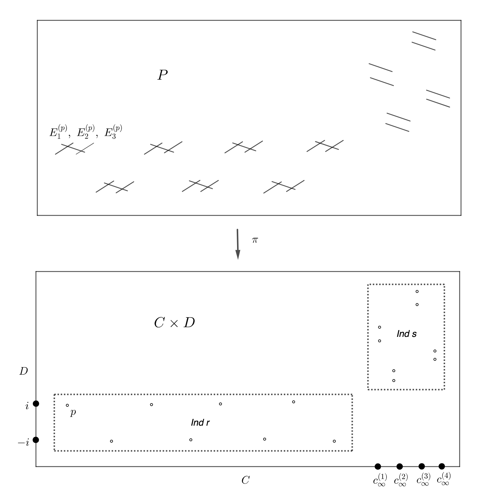
Figure 3. Model $P$, $d=4$.

To study the case of even degree $d$, we will require a model that has an analogue of the midpoint divisor. We therefore introduce the following variant of $P$. (We suggest skipping all arguments specific to the even case on first reading; they are conceptually identical to the odd case, but with more bookkeeping.)

Definition 3.5 (Model $P_{+}$).

Suppose $d$ is even. Let $p\in\operatorname{Ind}r$. Let $a^{(p)}=E_{d/2-1}^{(p)}\cap E_{d/2}^{(p)}$. Let $\tilde{\pi}^{(p)}_{+}:P_{+}^{(p)}\to P$ be the simple point blowup of $P$ at $a^{(p)}$. Let $\tilde{\pi}_{+}:P_{+}\to P$ be the join of all the $\tilde{\pi}_{+}^{(p)}$, and let $\pi_{+}=\pi\circ\tilde{\pi}_{+}$. Let $\mathcal{E}_{+}$ be the set of irreducible components of $\pi_{+}^{-1}(\operatorname{Ind}r\cup\operatorname{Ind}s)$, and let $\mathcal{E}^{(p)}_{+}$ be the subset of $\mathcal{E}_{+}$ over a given point $p$. See Figure 4.

Given $p\in\operatorname{Ind}r$, the midpoint divisor above $p$ is

$$E_{\operatorname{mid}}=E_{\operatorname{mid}}^{(p)}\colonequals\tilde{\pi}_{+}^{-1}(a^{(p)}).$$

Let

$$\hat{b}_{+},\hat{r}_{+},\hat{s}_{+}\colon P_{+}\vdash P_{+},$$

$$\hat{b}_{+}\colonequals\pi_{+}^{-1}\circ b\circ\pi_{+},\quad\hat{r}\colonequals\pi_{+}^{-1}\circ r\circ\pi_{+},\quad\hat{s}\colonequals\pi_{+}^{-1}\circ s\circ\pi_{+}.$$

We let

$$\beta_{+}\colonequals\hat{b}_{+}|_{E_{\operatorname{mid}}\vdash E_{\operatorname{mid}}},\quad\rho_{+}\colonequals\hat{r}_{+}|_{E_{\operatorname{mid}}\vdash E_{\operatorname{mid}}},\quad\sigma_{+}\colonequals\hat{s}_{+}|_{E_{\operatorname{mid}}\vdash E_{\operatorname{mid}}}.$$

Note that all the blowups in the definition of $P$ are free rather than satellite. That is, we only blow up centers that belong to one exceptional divisor (rather than two) at that stage. The blowup $\tilde{\pi}_{+}$ is satellite. From the Favre-Jonsson point of view [FJ04, Chapter 6], the divisor $E_{\operatorname{mid}}^{(p)}$ is the vertex of the relative universal dual graph that parametrizes Puiseux series of the form $y=uz^{(d-1)/2}$.

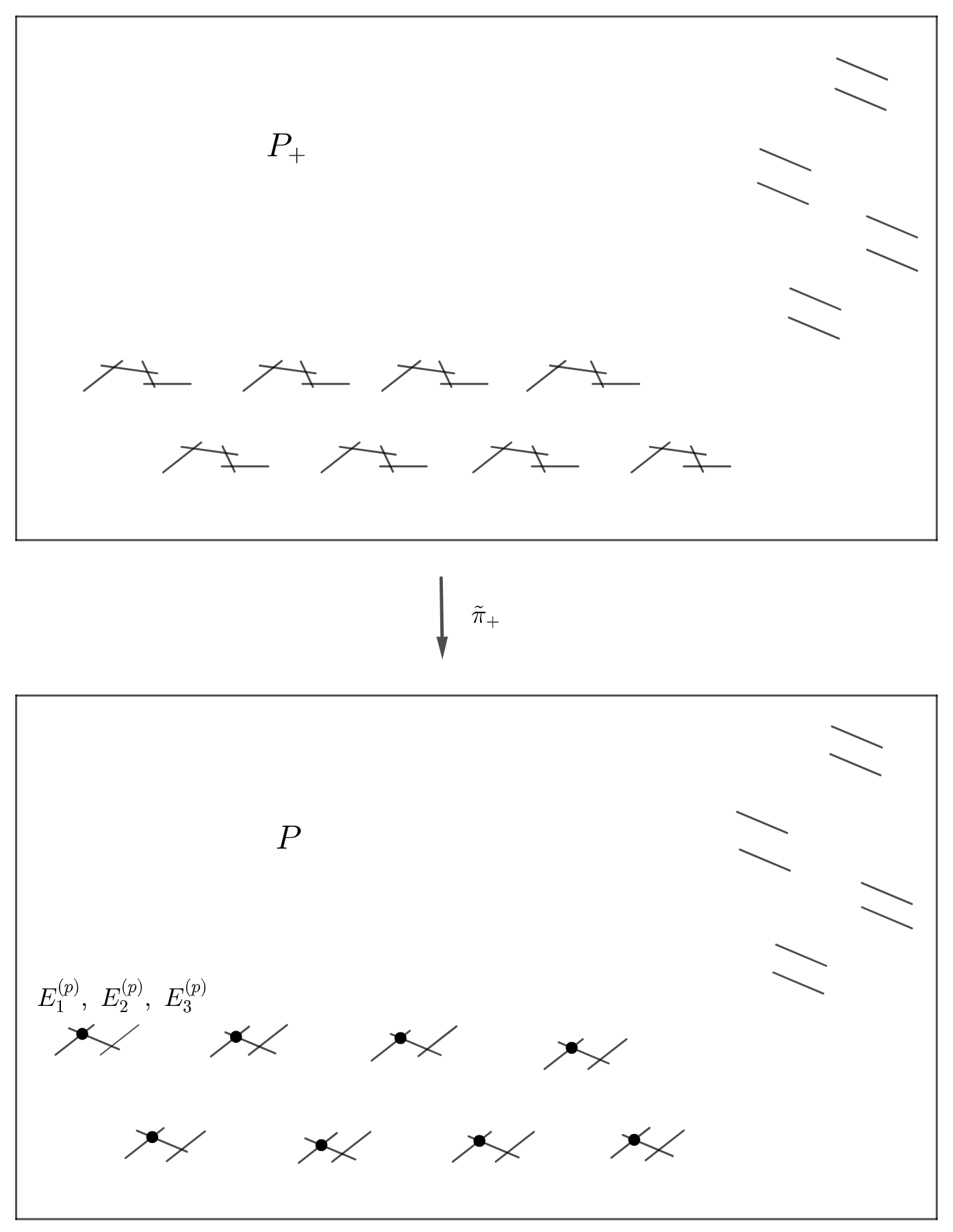
Figure 4. Model $P_{+}$, $d=4$. The marked points are blowup centers.

3.5. A double cover trick

In order to avoid using Puiseux series, when $d$ is even, we will study $P$ and $P_{+}$ using a kind of local double cover. This section should be skipped on first reading since it is relevant only to our proofs when $d$ is even.

Let $p\in\operatorname{Ind}r$. Let $G$ be the formal neighborhood of $C\times D$ about $p$. We construct a double cover of $G$ as follows. By an automorphism, assume $p=p_{1}^{(i)}=[1:-i:2]$, so $G$ is isomorphic to $(\mathbb{A}^{2},0)$ with the coordinates $y,z$ defined in (3.3).

Let $\tilde{G}=\tilde{G}^{(p)}=(\mathbb{A}^{2},0)$ with coordinates $(\tilde{y},\tilde{z})$, equipped with a $2$-to-$1$ map

$$\delta:\tilde{G}\to G,$$

$$(\tilde{y},\tilde{z})\mapsto(\tilde{y},\tilde{z}^{2}).$$

Let $\tau:\tilde{P}^{(p)}\to\tilde{G}$ denote the $(2d-2)$-fold iterated blowup defined using the process in Definition 3.4, with respect to $\tilde{y},\tilde{z}$. That is, we add divisors $\tilde{E}_{k}$ to $\tilde{G}$ for all $1\leq k\leq 2d-2$ parametrizing formal curves $\tilde{y}=\tilde{u}_{k}\tilde{z}^{k}$. Here $\tilde{u}_{k}$ is the preferred affine coordinate on $\tilde{E}_{k}$. There is an induced generically $2$-to-$1$ regular map

$$\delta_{1}:\tilde{P}^{(p)}\to P^{(p)}$$

sending $\tilde{E}_{k}$ to $E_{k/2}$ for all even $k$, and contracting $\tilde{E}_{k}$ to $E_{(k-1)/2}\cap E_{(k+1)/2}$ for all odd $k$. Further, there is a map

$$\delta_{2}:\tilde{P}^{(p)}\to P_{+}^{(p)}$$

that agrees with $\delta_{1}$ except that $\delta_{2}$ maps $\tilde{E}_{d-1}$ onto $E_{\operatorname{mid}}$. There is an affine coordinate $u$ on $E_{\operatorname{mid}}$ such that $\delta_{2}(\tilde{u}_{d-1})=\tilde{u}^{2}_{d-1}.$

Let

$$s_{2}=\delta^{\operatorname{adj}}\circ s\circ\delta,$$

$$r_{2}=\delta^{\operatorname{adj}}\circ r\circ\delta,$$

$$\tilde{s}=\tau^{-1}\circ s_{2}\circ\tau,$$

$$\tilde{r}=\tau^{-1}\circ r_{2}\circ\tau.$$

Then $\delta_{2}$ semiconjugates $\tilde{s}$ to $\hat{s}_{+}$, and $\tilde{r}$ to $\hat{r}_{+}$.

4. Reflection on models $P$ and $P_{+}$

Recall that $\pi:P\to C\times D$ and $\pi_{+}:P_{+}\to C\times D$ ($d$ even) are the models defined in Definition 3.4, 3.5. We show that the conjugates $\hat{r}$, $\hat{r}_{+}$ of $r$ to these models are biregular.

4.1. Reflection on $P$

In this section, we check that $\hat{r}:P\dashrightarrow P$ is biregular.

For each $p^{(\pm i)}_{j}=(c^{(\pm i)}_{j},\pm i)\in\operatorname{Ind}r$, let $D^{(\pm i)}_{j}\colonequals(c^{(\pm i)}_{j}\times D)$. The contractions of $r:C\times D\dashrightarrow C\times D$ are the curves

$$D^{(\pm i)}_{j}\times p_{j}^{(\pm i)}.$$

Therefore, to show that $\hat{r}$ has no contractions, we must check that none of the strict transforms $(\pi^{-1})_{\operatorname{str}}(D^{(\pm i)}_{j})$ and no exceptional primes in $\mathcal{E}$ are $\hat{r}$-contracted.

To handle the exceptional primes above $\operatorname{Ind}s$, we appeal to the following lemma.

Lemma 4.1 ([Wei23, Lemma 6.4]).

Let $p\in\operatorname{Ind}s$, and let $E=E^{(p)}$ be the exceptional prime divisor above $p$. Then

$$\operatorname{Ind}\hat{r}\cap E=\varnothing,$$

$$\hat{r}(E)=E,$$

$$\hat{r}_{*}E=E.$$

Proof.

The result holds for any smooth curve for which all scratch points at infinity are basic. (The proof, given in [Wei23], requires computing $\hat{r}(E)$ in local coordinates.) We showed that all scratch points at infinity are basic for the Fermat hyperbola in Section 3.2. ∎

This leaves the $(\pi^{-1})_{\operatorname{str}}(D^{(\pm i)}_{j})$ and the $E^{(p)}_{k}$ above $p\in\operatorname{Ind}r$ as the remaining possibly contracted curves. To show that these curves are not contracted, we compute their strict transforms.

Lemma 4.2.

Let $p=p^{(\pm i)}_{j}\in\operatorname{Ind}r$, and let $\hat{D}^{(\pm i)}_{j}={(\pi^{-1})_{\operatorname{str}}}(D^{(\pm i)}_{j})$. Then,

(9) $$\hat{r}_{\operatorname{str}}(\hat{D}^{(\pm i)}_{j})=E^{(p)}_{d-1},$$

(10) $$\hat{r}_{\operatorname{str}}(E^{(p)}_{d-1})=\hat{D}^{(\pm i)}_{j}.$$

Proof.

The claim reduces to the case $p=p^{(i)}_{1}=[1:-i:2]$, since by Lemma 3.1 and construction of $P$, an automorphism of $P$ takes $p^{(\pm i)}_{j}$ to $p^{(i)}_{1}$, $\hat{D}^{(\pm i)}_{j}$ to $\hat{D}^{(i)}_{1}$, and $E^{(p^{(\pm i)}_{j})}_{d-1}$ to $E^{(p^{(i)}_{1})}_{d-1}$. So let $p=p^{(i)}_{1}$ and consider the formal neighborhood $G$ around $p$ with the $yz$-coordinates defined in (3.3). Applying Proposition 3.3(1), the total composite graph of $(\pi_{d-1})^{-1}$ and $r$ (Definition 2.6) has local equations

$$z =v^{\prime},$$

$$\frac{z^{d-1}+O(z^{d})}{y} =(v^{\prime})^{d-1}u^{\prime}$$

$$=z^{d-1}u^{\prime}.$$

Therefore the graph of $\pi_{d-1}^{-1}\circ r$ has local equations

$$z =v^{\prime},$$

$$1+O(z) =yu^{\prime}.$$

So $(\pi_{d-1})^{-1}\circ r$ maps the germ of $\{z=0\}$ about $(y,z)=(0,0)$ onto a germ of $E_{d-1}$. Thus, $\pi_{d-1}^{-1}\circ r$ maps $\{z=0\}$, the formal curve represented by $D^{(i)}_{1}$, onto $\{v^{\prime}=0\}$, which is an affine equation for $E_{d-1}$. The strict transform of an irreducible curve by a birational map is irreducible with multiplicity $1$, so

$$(\pi^{-1}_{d-1}\circ r)_{\operatorname{str}}(D^{(i)}_{1})=E_{d-1}.$$

Since $\hat{D}^{(i)}_{1}=(\pi^{-1})_{\operatorname{str}}(D^{(i)}_{1})$, this proves (9). Since $\hat{r}$ is an involution, (9) implies (10). ∎

Lemma 4.2 may be interpreted as saying that $\hat{r}$ exchanges two points in the relative dual graph of an iterated blowup. Unsurprisingly, the map reverses the segment with those endpoints, as shown by the following lemma.

Lemma 4.3.

Let $p\in\operatorname{Ind}r$, and let $k\in\mathbb{N}$ be in the range $1\leq k\leq d-2.$ Then,

$$\hat{r}_{\operatorname{str}}(E_{k}^{(p)})=E_{d-1-k}^{(p)}.$$

On the midpoint divisor,

(11) $$\rho(u) =\frac{1}{u}.$$

Proof.

As before, assume $p=p^{(i)}_{1}$. We claim that

$$(\pi_{d-1-k}^{-1}\circ r\circ\pi_{k})_{\operatorname{str}}(E_{k})=E_{d-1-k}.$$

The total composite graph of $r$ and $\pi_{k}$ has local formal equations

$$v =z^{\prime},$$

$$y^{\prime}v^{k}u =(z^{\prime})^{d-1}+O((z^{\prime})^{d})$$

$$=v^{d-1}+O(v^{d}).$$

So $\Gamma_{r\circ\pi_{k}}$ has local formal equations

$$v =z^{\prime},$$

$$y^{\prime}u =v^{d-1-k}+O(v^{d-k}).$$

Then the total composite graph of $\pi_{d-1-k}^{-1}$ and $r\circ\pi_{k}$ has local equations

$$v =v^{\prime},$$

$$u^{\prime}v^{d-1-k}u =v^{d-1-k}+O(v^{d-k})$$

$$=(v^{\prime})^{d-1-k}+O((v^{\prime})^{d-k}).$$

So $\Gamma_{\pi_{d-1-k}^{-1}\circ r\circ\pi_{k}}$ maps $\{v=0\}$ to $\{v^{\prime}=0\}$.

Then (11) follows from choosing $k=(d-1)/2.$ ∎

Collecting these results yields the following proposition.

Proposition 4.4.

The birational map $\hat{r}:P\dashrightarrow P$ is biregular.

Proof.

Since $\hat{r}=\hat{r}^{-1}$, we have $\operatorname{Ind}\hat{r}=\operatorname{Exc}\hat{r}$. Combining Lemma 4.1, Lemma 4.2, and Lemma 4.3, we see that the strict transform of a curve by $\hat{r}$ is always $1$-dimensional. Since $\hat{r}$ is birational, by Lemma 2.9 there are no $\hat{r}$-contracted curves, so $\operatorname{Exc}\hat{r}=\varnothing$. ∎

4.2. Reflection on $P_{+}$

Say $d$ is even. Then we can study $P_{+}$. (This section may be skipped on first reading.)

The results of Lemmas 4.1, 4.2, and the first claim of Lemma 4.3 hold verbatim for $\hat{r}_{+}$ because all the computations are in local coordinates and can be done generically on the divisors. Let us prove the remaining claim about the midpoint divisor.

Lemma 4.5.

On the midpoint divisor, we have

(12) $$(\hat{r}_{+})_{\operatorname{str}}E_{\operatorname{mid}}=E_{\operatorname{mid}}$$

and

(13) $$\rho_{+}(u)=\frac{1}{u}.$$

Proof.

Employing the notation of Section 3.5, local equations for $r_{2}$ are obtained by substituting $y=\tilde{y},z=\tilde{z}^{2}$ in Proposition 3.3 (1). We get

$$\tilde{z}^{2}=\tilde{z}^{\prime 2},$$

$$\tilde{z}^{2d-2}(1+O(\tilde{z}^{2d}))=\tilde{y}\tilde{y}^{\prime}.$$

Changing coordinates as in Lemma 4.3, we get a multiplicity-$2$ equation for $\tilde{r}|_{\tilde{E}_{d-1}\vdash\tilde{E}_{d-1}}$,

$$\tilde{u}_{d-1}\tilde{u}_{d-1}^{\prime}=1.$$

Semiconjugating by $\delta_{2}$, the equation for $\hat{r}_{+}|_{E_{\operatorname{mid}}\vdash E_{\operatorname{mid}}}$ is $uu^{\prime}=1$, proving (12) and the formula for $\rho_{+}$. ∎

Gathering these results gives:

Proposition 4.6.

The map $\hat{r}_{+}:P_{+}\dashrightarrow P_{+}$ is biregular.

5. Secant on models $P$ and $P_{+}$

In this section, we compute the contracted curves and indeterminacy of $\hat{s}:P\vdash P$ and $\hat{s}_{+}:P_{+}\vdash P_{+}$, essentially by computing the images of all the exceptional divisors in our models. The subtle part of this description is for the exceptional divisors in $\mathcal{E}^{(p)}$, where $p\in\operatorname{Ind}r$. If we think of the dual graph of $\mathcal{E}^{(p)}$ as a segment, the basic picture can be summarized as follows: one part of the segment is contracted onto $E_{\operatorname{mid}}$, while the other part is invariant. Note that $s$ is multivalued, so it induces a multivalued map on the segment.

The contractions of $s:C\times D\vdash C\times D$ are all of the form

$$C_{j}\colonequals(C\times q_{j})\times(c_{j},q_{j}),$$

where $p_{j}=(c_{j},q_{j})\in\operatorname{Ind}s$, or equivalently $c_{j}\in C_{\infty}$, and $t(c_{j})=[q_{j}]$.

Let $\hat{C}_{j}\colonequals(\pi^{-1})_{\operatorname{str}}(C_{j})$. We studied the $\hat{C}_{j}$ and divisors above $\operatorname{Ind}s$ in our previous work.

Lemma 5.1 ([Wei23, Lemma 6.2]).

Let $E^{(p_{j})}\subset P$ be the exceptional prime above a point $p_{j}\in\operatorname{Ind}s$. Then $\hat{C}_{j}$ and $E^{(p_{j})}$ are not $\hat{s}$-contracted curves, and

$$\hat{s}_{*}E^{(p_{j})}=\hat{s}_{\operatorname{str}}(E^{(p_{j})})=\hat{C}_{j}.$$

Proof.

In [Wei23, Lemma 6.2], we calculated that $\hat{s}|_{\hat{C}_{j}\vdash E^{(p_{j})}}$ is $(d-1)$-to-$1$, and it follows from the definition of $s$ that $\hat{s}|_{\hat{C}_{j}\vdash\hat{C}_{j}}$ is $(d-2)$-to-$(d-2)$. So, by the contracted curve test (Lemma 2.9), the curve $\hat{C}_{j}$ is not $\hat{s}$-contracted.

Since $\hat{s}|_{E^{(p_{j})}\vdash\hat{C}_{j}}$ is $1$-to-$(d-1)$ by symmetry, we have $\hat{s}_{\operatorname{str}}(E^{(p_{j})})=\hat{C}_{j}$ by counting images, and Lemma 2.9 shows that $E^{(p_{j})}$ is not $\hat{s}$-contracted. Since $\operatorname{Ind}\hat{s}\cap\hat{C}_{j}=\varnothing$ [Wei23, Lemma 6.2], we obtain $\hat{s}_{*}E^{(p_{j})}=\hat{s}_{\operatorname{str}}(E^{(p_{j})})$ since pushforward and strict transform agree modulo exceptional image curves. ∎

It follows that $s$ lifts to a biregular correspondence on the blowup of $C\times D$ at every point of $\operatorname{Ind}s$. The key question is how $s$ behaves above $\operatorname{Ind}r$. Let us examine the aforementioned “invariant” part.

Lemma 5.2.

Let $p\in\operatorname{Ind}r$, and let $E_{k}=E_{k}^{(p)}$, where $k\in\mathbb{N}$ is in $\frac{d-1}{2}<k\leq d-1$. Then,

$$\hat{s}_{\operatorname{str}}(E_{k})=(d-1)E_{k}.$$

Proof.

It suffices to show that $\deg_{1}(\hat{s}|_{E_{k}\vdash E_{k}})=d-1$, since then by counting images there can be no more curves in $\hat{s}_{\operatorname{str}}(E_{k})$. By applying an automorphism as before, we may assume $p=p_{1}=[1:-i:2]$. We claim that

$$(\pi_{k}^{-1}\circ s\circ\pi_{k})_{\operatorname{str}}(E_{k})=(d-1)E_{k}.$$

The total composite graph of $s$ and $\pi_{k}$ has equations

$$y^{\prime} =uv^{k},$$

$$2d(uv^{k})^{2} =v^{d-1}+v^{d-2}z^{\prime}+\ldots+(z^{\prime})^{d-1}+A(v,z^{\prime}),$$

by Proposition 3.3 (2). The total composite graph has no non-dominant components, since these would lie above $\{v=0\}$ or $\{u=0\}$. So $\Gamma_{s\circ\pi_{k}}$ has the same equations. The total composite graph of $\pi_{k}^{-1}$ and $s\circ\pi_{k}$ is then

$$u^{\prime}(v^{\prime})^{k} =uv^{k},$$

(14) $$2d(uv^{k})^{2} =v^{d-1}+v^{d-2}v^{\prime}+\ldots+(v^{\prime})^{d-1}+A(v,v^{\prime}).$$

Since $A(v,v^{\prime})\in\langle v,v^{\prime}\rangle^{d}$ and $k>\frac{d-1}{2}$, we may rewrite (5) as a product of formal series

$$0=\prod_{\begin{subarray}{c}\eta:\eta^{d}=1\\ \eta\neq 1\end{subarray}}(v^{\prime}-\eta v+O(v^{2})),$$

where $O(v^{2})$ denotes an element of $\langle v\rangle^{2}\subset{\mathbf{k}}[u][[v]]$. That is, the ideal of the total composite graph of $\pi_{k}^{-1}$ and $s\circ\pi_{k}$ factors as

$$\prod_{\begin{subarray}{c}\eta:\eta^{d}=1\\ \eta\neq 1\end{subarray}}I_{\eta},$$

where $I_{\eta}$ is an ideal of the form

$$\langle u^{\prime}(v^{\prime})^{k}-uv^{k},v^{\prime}-\eta v+O(v^{2})\rangle\cong\langle u^{\prime}(\eta v)^{k}-uv^{k}+O(v^{2k})\rangle\subseteq{\mathbf{k}}[u,u^{\prime}][[v]].$$

Dividing through by $v^{k}$ gives the ideal $\langle u^{\prime}\eta^{k}-u+O(v)\rangle$, which defines a $1$-to-$1$ correspondence from $E_{k}$ to $E_{k}$. There are $d-1$ factors, hence the result. ∎

5.1. Secant, odd case

The behavior of secant on $P$ depends on parity. In this subsection, we assume that the degree $d$ is odd. Recall that this allows us to define the midpoint divisor in $P$ above $p\in\operatorname{Ind}r$,

$$E_{\operatorname{mid}}^{(p)}=E^{(p)}_{(d-1)/2}.$$

We identify $E_{\operatorname{mid}}$ with $\mathbb{P}^{1}$ by the map $u:E_{\operatorname{mid}}^{\circ}\to\mathbb{A}^{1}$, see Definition 3.4. The point $a=E_{\operatorname{mid}}\cap E_{(d-1)/2-1}$ is identified with $\infty$ in $\mathbb{P}^{1}$.

Lemma 5.3.

The correspondence $\sigma$ is $(d-1)$-to-$(d-1)$. If $u_{0}\in{\mathbf{k}}$, then

(15) $$\sigma(u_{0})=\left\{\frac{u_{0}}{\alpha^{(d-1)/2}}:\;\alpha\in{\mathbf{k}},\;\alpha^{d-1}+\ldots+1-2du_{0}^{2}=0\right\}.$$

The image of $\infty$ is $\sigma(\infty)=\{\pm\sqrt{1/2d}\}$, each with multiplicity $(d-1)/2$.

Proof.

By Proposition 3.3 (2), the total transform of $\Gamma_{s}$ to $P\times P$ has local analytic equations on a neighborhood of $E_{\operatorname{mid}}^{\circ}\times E_{\operatorname{mid}}^{\circ}$ given by

$$uv^{(d-1)/2} =u^{\prime}(v^{\prime})^{(d-1)/2},$$

$$2du^{2}v^{d-1} =v^{d-1}+\ldots+(v^{\prime})^{d-1}+O((v,v^{\prime})^{d}).$$

Let $\alpha=v^{\prime}/v$. Then in coordinates $u,u^{\prime},\alpha,v$, the graph is given by

$$uv^{(d-1)/2} =u^{\prime}v^{(d-1)/2}\alpha^{(d-1)/2},$$

$$2du^{2}v^{d-1} =v^{d-1}(\alpha^{d-1}+\ldots+1+O(v)).$$

Thus the strict transform of $\Gamma_{s}$ restricted to $\{v=0\}$ is

$$u =u^{\prime}\alpha^{(d-1)/2},$$

(16) $$2du^{2} =\alpha^{d-1}+\ldots+1.$$

This proves (15). By self-adjointness of $\hat{s}$, $\sigma(\infty)=\sigma^{\operatorname{adj}}(\infty)$. If $u_{0}\in{\mathbf{k}}$, and $\sigma(u_{0})$ is finite, then $0$ is a root of $\alpha^{d-1}+\ldots+1-2du_{0}^{2}$ as a polynomial in $\alpha$, so $u_{0}\in\{\pm\sqrt{1/2d}\}$. So it remains to show that $\infty$ is not in $\sigma(\infty)$.

By (16), we have $0=1+\ldots+1/\alpha^{d-1}-2d(u^{\prime})^{2}$ for any $u^{\prime}$ finite in $\sigma(u)$. As $u\to\infty$, we therefore get $\alpha\to\infty$, so $u^{\prime}\to\pm\sqrt{1/2d}$. The multiplicities follow by Galois symmetry. ∎

The next lemma is the main result of this section. It classifies indeterminacy points of $\hat{s}$.

Lemma 5.4.

Say $d$ is odd. The $\hat{s}$-contracted curves and $\hat{s}$-exceptional image curves are the divisors $E^{(p)}_{k}$, $p\in\operatorname{Ind}r$, $1\leq k<(d-1)/2$. For each $p\in\operatorname{Ind}r$,

$$\operatorname{Ind}\hat{s}\cap\mathcal{E}^{(p)}\subset E^{(p)}_{\operatorname{mid}},$$

and with the identification $u:E^{(p)}_{\operatorname{mid}}\to\mathbb{P}^{1}$,

$$\operatorname{Ind}\hat{s}\cap\mathcal{E}^{(p)}=\sigma(\infty)=\{\pm\sqrt{1/2d}\}.$$

For each $u_{0}\in\operatorname{Ind}\hat{s}\cap\mathcal{E}^{(p)}$, we have

$$\hat{s}(u_{0})=\bigcup_{1\leq k<(d-1)/2}E^{(p)}_{k}.$$

Proof.

Fix $p\in\operatorname{Ind}r$. We argue by descending induction on $k$, from $k=(d-1)/2-1$ to $1$. Since $s(p)=\{p\}$, we have $\hat{s}(E_{k}^{(p)})\subset\mathcal{E}^{(p)}$. Let $k=(d-1)/2-1$, $a^{(p)}\colonequals E^{(p)}_{(d-1)/2-1}\cap E^{(p)}_{\operatorname{mid}}$. So $u(a^{(p)})=\infty$. We claim we cannot have $E^{(p)}_{\operatorname{mid}}\subset\hat{s}(E^{(p)}_{(d-1)/2-1})$. By Lemma 5.2, a general point of $E_{\operatorname{mid}}$ has a discrete set of at least $d-1$ preimages in $E_{\operatorname{mid}}$ with multiplicity, none of them $\infty$. Having a further preimage is not possible by Stein (Lemma 2.5). Thus $\hat{s}(E^{(p)}_{(d-1)/2-1})$ contains $\sigma(\infty)$ as a discrete set, with total multiplicity $d-1$. It follows, again by Lemma 2.5, that $\hat{s}(E_{(d-1)/2-1})$ contains no other points. So $\hat{s}(E^{(p)}_{(d-1)/2-1})=\sigma(\infty)$. Repeating this argument for $k-1$, we find that $\hat{s}(E^{(p)}_{k-1})\subset\hat{s}(E^{(p)}_{k-1}\cap E^{(p)}_{k})=\operatorname{Ind}\hat{s}$ with images of total multiplicity $d-1$, etc. ∎

Remark 5.5.

One also may show that the $E_{k}^{(p)}$, $k>(d-1)/2$ are not $\hat{s}$-contracted or $\hat{s}$-exceptional image curves via Lemma 5.2 and the contracted curve test, Lemma 2.9.

Corollary 5.6.

For $d=2$ and $d=3$, the correspondence $\hat{b}:P\vdash P$ is biregular, that is, $\operatorname{Ind}\hat{b}=\operatorname{Exc}\hat{b}=\varnothing$.

In the case $d=2$, the definitions of $P$ and the modified phase space $P_{\operatorname{gen}}$ coincide, and the result was proved as [Wei23, Corollary 7.11].

Proof.

The correspondence $\hat{r}:P\to P$ is biregular (Proposition 4.4). By Lemma 5.4, the contracted and exceptional image curves of $\hat{s}$ are $\{E^{(p)}_{k}:p\in\operatorname{Ind}r,1\leq k<(d-1)/2\}$. If $d\leq 3$, this set is empty, so $\hat{s}$ is biregular. Then $\hat{b}$ is biregular. ∎

5.2. Secant, even case

In this subsection, we assume that the degree $d$ is even. This allows us to define $P_{+}$ and the “midpoint divisor” $E_{\operatorname{mid}}^{(p)}$ in $P_{+}$ above any $p\in\operatorname{Ind}r$. To study this divisor, we employ the double cover defined in Section 3.5. This section may be skipped on first reading.

Lemmas 5.1 and 5.2 hold verbatim for $\hat{s}_{+}$, again because these computations are local and computable generically on the divisors. Let us prove the analogue of Lemma 5.3.

Let $\sigma_{+}\colonequals\hat{s}_{+}|_{E_{\operatorname{mid}}\vdash E_{\operatorname{mid}}}.$

Lemma 5.7.

The correspondence $\sigma_{+}$ is $(d-1)$-to-$(d-1)$, given by the formula

(17) $$\sigma_{+}(u)=\left\{\frac{u}{\alpha^{d-1}}:\alpha\in{\mathbf{k}},\;\alpha^{d-1}+\ldots+1-2du\right\},$$

and $\sigma_{+}(\infty)=\{1/2d\}$.

Proof.

Local equations for $s_{2}$ are obtained by substitution into Proposition 3.3 (2):

$$\tilde{y}=\tilde{y}^{\prime},$$

$$2d\tilde{y}^{2}=\tilde{z}^{2d-2}+\tilde{z}^{2d-4}\tilde{z}^{\prime 2}+\ldots+\tilde{z}^{\prime 2d-2}+A(\tilde{z}^{2d},\tilde{z}^{\prime 2d}).$$

Calculating the strict transform as in the proof of Lemma 5.3 gives local equations for $\tilde{s}|_{\tilde{E}_{d-1}\vdash\tilde{E}_{d-1}}$:

$$\tilde{u}=\tilde{u}^{\prime}\tilde{\alpha}^{d-1},$$

$$2d\tilde{u}^{2}=\tilde{\alpha}^{2d-2}+\tilde{\alpha}^{2d-4}+\ldots+1,$$

so again following our previous argument, we get $\tilde{s}|_{\tilde{E}_{d-1}\vdash\tilde{E}_{d-1}}(\infty)=\{\pm 1/\sqrt{2d}\}$. Then, by semiconjugacy, we obtain that $\sigma_{+}$ is $(d-1)$-to-$(d-1)$ and $\sigma_{+}(\infty)=\{1/2d\}$. Finally, (17) follows by semiconjugacy from the equations for $\tilde{s}|_{\tilde{E}_{d-1}\vdash\tilde{E}_{d-1}}$. ∎

Lemma 5.8.

The $\hat{s}_{+}$-contracted curves and $\hat{s}_{+}$-exceptional image curves are the divisors $E^{(p)}_{k}$, $1\leq k<(d-1)/2$. For each $p\in\operatorname{Ind}r$,

$$\operatorname{Ind}\hat{s}_{+}\cap\mathcal{E}_{+}^{(p)}\subset E^{(p)}_{\operatorname{mid}},$$

$$\operatorname{Ind}\hat{s}_{+}\cap\mathcal{E}_{+}^{(p)}=\sigma_{+}(\infty)=\{1/2d\}.$$

For each $u_{0}\in\operatorname{Ind}\hat{s}_{+}\cap\mathcal{E}_{+}^{(p)}$, we have

$$\hat{s}_{+}(u_{0})=\bigcup_{1\leq k\leq(d-1)/2}E^{(p)}_{k}.$$

Proof.

Follows from Lemma 5.7 using the proof of Lemma 5.4. ∎

Lemma 5.9.

Say $d$ is even. The $\hat{s}$-contracted curves and $\hat{s}$-exceptional image curves of $P$ are the divisors $E^{(p)}_{k}$, $1\leq k<(d-1)/2$. For each $p\in\operatorname{Ind}r$,

$$\operatorname{Ind}\hat{s}\cap\mathcal{E}^{(p)}=E^{(p)}_{d/2-1}\cap E^{(p)}_{d/2},$$

$$\hat{s}(E^{(p)}_{d/2-1}\cap E^{(p)}_{d/2})=\bigcup_{1\leq k<(d-1)/2}E^{(p)}_{k}.$$

Proof.

Follows from Lemma 5.8 after contracting $E_{\operatorname{mid}}$. (Note that Lemma 5.7 shows that $\sigma_{+}$ is $(d-1)$-to-$(d-1)$.) ∎

6. The dynamical degree

Usually, one calculates the dynamical degree of a correspondence by constructing an algebraically stable model. The issue in our case is that the construction of such a model seems to depend in some delicate way on characteristic. In Section 7, we show that the model $P$ (resp. $P_{+}$) is algebraically stable if ${\mathbf{k}}=\mathbb{C}$ when $d\geq 3$ is odd (resp. even), but it is not hard to check using our formulas for $\sigma$ and $\rho$ that this can fail in positive characteristic, e.g. when $d$ is odd and $\operatorname{char}{\mathbf{k}}$ divides $2d-1$. Solving this problem would require a far more sophisticated understanding of finite characteristic dynamics than is presently available.

Instead, we take a different tack. We show that, regardless of parity of $d$, the model $P$ has the essential feature of an algebraically stable model that allows us to calculate dynamical degrees.

Definition 6.1.

Let $f:X\vdash X$ be a dominant correspondence on a smooth irreducible projective surface $X$. We say $f$ is essentially stable if there exists a big-and-nef divisor $\Delta$ on $X$ such that, for all $n\in\mathbb{N}$,

$$\left(f^{n}\right)_{*}\Delta\cdot\Delta=(f_{*})^{n}\Delta\cdot\Delta.$$

This property is a weakening of algebraic stability that still permits computation of the dynamical degree, as shown by the following lemma.

The spectral radius of a linear endomorphism $T$ is $\operatorname{rad}T\colonequals\max_{\lambda}\left|\lambda\right|,$ where $\lambda$ ranges over the eigenvalues of $T$.

Lemma 6.2.

If $f:X\vdash X$ is essentially stable, then

$$\lambda_{1}(f)=\operatorname{rad}f_{*}.$$

Proof.

Let $\Delta$ be a big-and-nef divisor witnessing essential stability. We claim the following circle of inequalities holds:

$$\lambda_{1}(f) \geq\lim_{n\to\infty}\left(\left(f^{n}\right)_{*}\Delta\cdot\Delta\right)^{1/n}$$

$$=\lim_{n\to\infty}\left(\left(f_{*}\right)^{n}\Delta\cdot\Delta\right)^{1/n}$$

$$=\operatorname{rad}f_{*}$$

$$\geq\lambda_{1}(f).$$

These estimates are all standard. The first line follows from expressing $\Delta$ as a difference of ample divisors. The second line is the hypothesis. To prove the third line, note that big-and-nef classes are in the interior of the pseudoeffective cone [Laz04], and $f_{*}$ preserves the pseudoeffective cone; then apply the Perron-Frobenius theorem for cone-preserving operators. The last line is the “first iterate estimate” for dynamical degrees [Wei23, Theorem 2.18(2)]. ∎

We now build up to showing that $\hat{b}$ is essentially stable. This is true whether $d$ is odd or even.

The idea for the proof is simple. The lack of algebraic stability of a correspondence $f$ is measured by $(f^{n})_{*}-(f_{*})^{n}$, whose image is supported on $f$-exceptional image curves and their strict iterates. In the case of $\hat{b}$, these curves are all contained in a subset of $\mathcal{E}$. Then any big-and-nef divisor $\Delta$ orthogonal to $\mathcal{E}$ suffices. (Our reason for working with big-and-nef divisors rather than ample divisors is that, by definition of amplitude, no ample divisor is orthogonal to $\mathcal{E}$.)

Let $W_{1}\subset\operatorname{Div}P$ be the subgroup generated by $\{E^{(p)}_{k}:1\leq k\leq d-2,\;p\in\operatorname{Ind}r\}$. Let $N_{1}$ be the image of $W_{1}$ in $\operatorname{Num}P$.

Lemma 6.3.

1. All exceptional image curves of $\hat{s},\hat{r},\hat{b}$ lie in $W_{1}$.

2. We have

   $$\hat{s}_{\operatorname{str}}(W_{1})\subseteq W_{1},\quad\hat{r}_{\operatorname{str}}(W_{1})\subseteq W_{1},\quad\hat{b}_{\operatorname{str}}(W_{1})\subseteq W_{1}.$$

3. We have

   $$\hat{s}_{*}(W_{1})\subseteq W_{1},\quad\hat{r}_{*}(W_{1})\subseteq W_{1},\quad\hat{b}_{*}(W_{1})\subset W_{1}.$$

4. We have

   $$\hat{s}_{*}(N_{1})\subseteq N_{1},\quad\hat{r}_{*}(N_{1})\subseteq N_{1},\quad\hat{b}_{*}(N_{1})\subset N_{1}.$$

Proof.

Claim (1) about $\hat{s}$ is by Lemma 5.4 (odd case), Lemma 5.9 (even case). Claim (2) about $\hat{s}$ is by Lemma 5.2 and Lemma 5.4.

Claim (1) about $\hat{r}$ is vacuous by Proposition 4.4. Claim (2) about $\hat{r}$ is by Lemma 4.3.

Claims (1) and (2) about $\hat{b}$ follow from those for $\hat{s}$ and $\hat{r}$.

Claim (3) follows from (1) and (2) because pushforward agrees with strict transform modulo exceptional image curves.

Claim (4) follows from (3) because pushforward respects the class map. ∎

Lemma 6.4.

For any divisor $\Delta\in\operatorname{Div}P$, and any $n\in\mathbb{N}$, we have

$$(\hat{b}^{n})_{*}\Delta\equiv(\hat{b}_{*})^{n}\Delta\mod W_{1}.$$

Proof.

We argue by induction. The case $n=1$ is trivial. Assuming the claim for $n$, we have

$$(\hat{b}^{n+1})_{*}\Delta \equiv\hat{b}_{*}(\hat{b}^{n})_{*}\Delta$$ (Lemma 6.3 (1)

$$\equiv\hat{b}_{*}(\hat{b}_{*})^{n}\Delta$$ (Lemma 6.3 (3))

$$\equiv(\hat{b}_{*})^{n+1}\Delta.$$

∎

Let $C_{0}$ and $D_{0}$ be divisors of the form $C\times q_{0}$ and $c_{0}\times D$, where $c_{0}\in C$, $q_{0}\in D$ are general. Let $\hat{C}_{0}=\pi^{*}C_{0},\hat{D}_{0}=\pi^{*}D_{0}$. Let $\Delta\colonequals\hat{C}_{0}+\hat{D}_{0}$.

Proposition 6.5 (essential stability).

The correspondence $\hat{b}:P\vdash P$ is essentially stable. It follows that

$$\lambda_{1}(b)=\lambda_{1}(\hat{b})=\operatorname{rad}\hat{b}_{*}.$$

Proof.

The divisor $\pi_{*}\Delta$ is nef since it intersects $C_{0}$ and $D_{0}$ with multiplicity $1$ each, and these are a basis of $\operatorname{Num}C\times D$. So the pullback $\Delta=\pi^{*}\pi_{*}\Delta$ is nef. To show that $\Delta$ is also big, we need $\Delta\cdot\Delta>0$. Since $\Delta$ is disjoint from the contracted curves of $\pi$, we have

$$\Delta\cdot\Delta=\pi_{*}\Delta\cap\pi_{*}\Delta=2>0.$$

By Lemma 6.4, for each $n\in\mathbb{N}$, we have

$$\left(\hat{b}^{n}\right)_{*}\Delta\in(\hat{b}_{*})^{n}\Delta+W_{1}.$$

Since $\Delta$ is intersection-orthogonal to $W_{1}$, intersecting against $\Delta$ proves that $\hat{b}$ is essentially stable.

Dynamical degrees are birational conjugacy invariants (Theorem 2.16 (1), so $\lambda_{1}(b)=\lambda_{1}(\hat{b})$. The remaining equality follows from Lemma 6.2. ∎

This completes the conceptual half of the proof of Theorem 1.2. Alas, now we must compute the entries and spectral radius of a square matrix of dimension $2+2d^{2}$, a matter of intersection theory and linear algebra. Fortunately, there are some tricks that reduce the dimension of the computation. (Notice that the value we ultimately obtain in Theorem 1.2 is at worst an algebraic integer of degree $2$ rather than $2+2d^{2}$.)

By Lemma 6.3 (4), the pushforwards $\hat{s}_{*},\hat{r}_{*},\hat{b}_{*}$ descend to endomorphisms of $(\operatorname{Num}P)/N_{1}$.

Rather than study the whole space $(\operatorname{Num}P)/N_{1}$, which has rank $2+4d$, it is more convenient to restrict our attention to just the divisors that show up when iterating $\hat{C}_{0}$ and $\hat{D}_{0}$. We set this up as follows.

Let $N$ be the smallest subspace of $\operatorname{Num}P$ that is closed under $\hat{s}_{*}$ and $\hat{r}_{*}$ and contains $\hat{C}_{0}$, $\hat{D}_{0}$, and $N_{1}$. Let $N_{0}\colonequals N/N_{1}$. The pushforward homomorphisms $\hat{b}_{*}$, $\hat{r}_{*}$ $\hat{s}_{*}:\operatorname{Num}P\to\operatorname{Num}P$ map $N$ into $N$ and $N_{1}$ into $N_{1}$. Hence there are endomorphisms $\overline{b}$, $\overline{r}$ $\overline{s}:N_{0}\to N_{0}$ induced by $\hat{b}_{*}|_{N}$, $\hat{r}_{*}|_{N}$, and $\hat{s}_{*}|_{N}$. Note that since $\hat{r}$ is regular, by Lemma 2.12, we have $\hat{b}_{*}=\hat{r}_{*}\hat{s}_{*}$, so $\overline{b}=\overline{r}\,\overline{s}$.

Proposition 6.6.

The group $N_{0}$ is a rank $4$ free abelian group generated by the classes of

$$\hat{C}_{0},\quad\hat{D}_{0},\quad E_{\infty}\colonequals\sum_{p\in\operatorname{Ind}s}E^{(p)},\quad F_{d-1}\colonequals\sum_{p\in\operatorname{Ind}r}E^{(p)}_{d-1}.$$

In this basis,

(18) $$\overline{r}=\begin{bmatrix}1&0&0&0\\ d(d-1)&1&0&2d\\ 0&0&1&0\\ -(d-1)&0&0&-1\end{bmatrix},\quad\overline{s}=\begin{bmatrix}d-1&2&d-1&0\\ 0&d-1&0&0\\ 0&-1&-1&0\\ 0&0&0&d-1\end{bmatrix},$$

(19) $$\overline{b}=\begin{bmatrix}d-1&2&2d&0\\ d^{3}-2d^{2}+d&2d^{2}-d-1&2d^{3}&2d^{2}-2d\\ 0&-1&-1&0\\ -(d-1)^{2}&-2d+2&-(2d-2)d&-(d-1)\end{bmatrix}.$$

To prove this, we show that, modulo $N_{1}$,

(20) $$\hat{r}_{*}\hat{C}_{0} \equiv\hat{C}_{0}+d(d-1)\hat{D}_{0}-(d-1)F_{d-1},$$

(21) $$\hat{r}_{*}\hat{D}_{0} \equiv\hat{D}_{0},$$

(22) $$\hat{r}_{*}E_{\infty} \equiv E_{\infty},$$

(23) $$\hat{r}_{*}F_{d-1} \equiv 2d\hat{D}_{0}-F_{d-1},$$

(24) $$\hat{s}_{*}\hat{C}_{0} \equiv(d-1)\hat{C}_{0},$$

(25) $$\hat{s}_{*}\hat{D}_{0} \equiv 2\hat{C}_{0}+(d-1)\hat{D}_{0}-E_{\infty},$$

(26) $$\hat{s}_{*}E_{\infty} \equiv(d-1)\hat{C}_{0}-E_{\infty},$$

(27) $$\hat{s}_{*}F_{d-1} \equiv(d-1)F_{d-1}.$$

We prove (20)-(27) in order.

Proof of (20).

Let $C^{\prime}\colonequals r_{*}C_{0}\in\operatorname{Div}C\times D$. By [Wei23, Equation 23], $C^{\prime}$ has bidegree $(1,d(d-1))$ in $\operatorname{Num}C\times D$. Therefore

$$\hat{r}_{*}\hat{C}_{0}=\hat{C}_{0}+d(d-1)\hat{D}_{0}-\sum_{E\in\mathcal{E}}m_{E}E,$$

where $m_{E}$ is the order of vanishing of $\pi^{*}C^{\prime}$ along $E$. Since $C^{\prime}\cap\operatorname{Ind}s=\varnothing$, we get $m_{E}=0$ for all $E$ above $\operatorname{Ind}s$. We are working modulo $N_{1}$, so we just need the vanishing order of $C^{\prime}$ on $E_{d-1}^{(p)}$, for each $p\in\operatorname{Ind}r$. By Proposition 3.3, if $p\in\operatorname{Ind}r$, then locally around $p$ in $(y,z)$ coordinates the equation of $C^{\prime}$ is of the form, for some $\kappa_{0}\neq 0$,

$$y=\kappa_{0}z^{d-1}+O(z^{d}).$$

This vanishes to order $d-1$ on $E_{d-1}^{(p)}$, since setting $y=uv^{d-1}$, $z=v$, the equation is sharply divided by $v^{d-1}$. ∎

Proof of (21).

Indeed $\hat{r}_{*}\hat{D}_{0}=\hat{D}_{0}$ as divisors, since $r_{*}D_{0}=D_{0}$ and $D_{0}\cap\operatorname{Ind}\pi=\varnothing$. ∎

Proof of (22).

Indeed $\hat{r}_{*}E_{\infty}=E_{\infty}$ as divisors (Lemma 4.1). ∎

Proof of (23).

In fact, we claim that for each $p\in\operatorname{Ind}r$, we have

$$\hat{r}_{*}(E_{d-1}^{(p)})\equiv D_{0}-E_{d-1}^{(p)}\mod N_{1}.$$

By symmetry, we can just consider $p=p^{(i)}_{1}$. By Lemma 4.2, we have

$$(r\circ\pi)_{*}E_{d-1}^{(p)}=D_{1}^{(i)},$$

which is of bidegree $(0,1)$. So

$$\hat{r}_{*}E_{d-1}^{(p)}=\hat{D}_{0}-\sum_{E\in\mathcal{E}}m_{E}E,$$

where $m_{E}$ is the order of vanishing of $\pi^{*}D_{1}^{(i)}$ along $E$. Since $D_{1}^{(i)}\cap(\operatorname{Ind}s\cup\operatorname{Ind}r)=\{p\}$, working modulo $N_{1}$, we just need to compute $m_{E_{d-1}^{(p)}}$. Writing $D_{1}^{(i)}$ locally at $p$ as $\{z=0\}$, $\pi^{*}D_{1}^{(i)}$ has local equation $\{v_{d-1}=0\}$ in $V^{\circ}_{\pi_{d-1}}$, same as $E^{(p)}_{d-1}$. ∎

Proof of (24).

Since $q_{0}$ is general, $s|_{C_{0}\vdash C_{0}}$ is $(d-1)$-to-$(d-1)$, so $s_{*}C_{0}=(d-1)C_{0}$. ∎

Proof of (25).

Let $D^{\prime}\colonequals s_{*}D_{0}\in\operatorname{Div}C\times D$. By [Wei23, Equation 22], $D^{\prime}$ has bidegree $(d-1,2)$ in $\operatorname{Num}C\times D$. Therefore

$$\hat{s}_{*}\hat{D}_{0}=(d-1)\hat{C}_{0}+2\hat{D}_{0}-\sum_{E\in\mathcal{E}}m_{E}E,$$

where $m_{E}$ is the order of vanishing of $\pi^{*}D^{\prime}$ along $E$.

Similarly, for each $p\in\operatorname{Ind}s$, we have $\hat{s}_{*}E^{(p)}=C_{0}-E^{(p)}$ in $\operatorname{Num}P$, since the divisor $(s\circ\pi)_{*}E^{(p)}$ is a smooth curve of bidegree $(1,0)$ such that $(s\circ\pi)_{*}E^{(p)}\cap(\operatorname{Ind}s\cup\operatorname{Ind}r)=\{p\}$ (Lemma 5.1).

Notice $D^{\prime}\cap(\operatorname{Ind}s\cup\operatorname{Ind}r)=\operatorname{Ind}s$. So in $\operatorname{Num}P$,

$$m_{E^{(p)}}=\hat{s}_{*}D_{0}\cdot E^{(p)} =D_{0}\cdot\hat{s}_{*}E^{(p)}$$ (by self-adjointness)

$$=D_{0}\cdot(C_{0}-E^{(p)})$$

$$=1.$$

∎

Proof of (26).

Again $\hat{s}_{*}E^{(p)}=C_{0}-E^{(p)}$ in $\operatorname{Num}P$ by Lemma 5.1 and linear equivalence. ∎

Proof of (27).

We have $\hat{s}_{\operatorname{str}}F_{d-1}=(d-1)F_{d-1}$ by Lemma 5.2. And $\hat{s}_{*}F_{d-1}-\hat{s}_{\operatorname{str}}F_{d-1}$ is supported on $\hat{s}_{*}$-exceptional image curves, which are in $W_{1}$ by Lemma 6.3 (1). ∎

We arrive at the proof of our main result.

Theorem 6.7 ($=$ Theorem 1.2).

The dynamical degree of the billiards correspondence $b:C\times D\vdash C\times D$ in the Fermat hyperbola is

$$\lambda_{1}(b)=\frac{2d^{2}-3d+\sqrt{(2d^{2}-3d)^{2}-4(d-1)}}{2}.$$

Proof.

By Proposition 6.5,

$$\lambda_{1}(b)=\lambda_{1}(\hat{b})=\operatorname{rad}\hat{b}_{*}.$$

We claim $\operatorname{rad}\hat{b}_{*}=\operatorname{rad}\overline{b}$. Since $\hat{b}_{*}|_{N_{0}}$ is semiconjugate to $\overline{b}$, see Proposition 6.6, we have

$$\operatorname{rad}\hat{b}_{*}\geq\operatorname{rad}\hat{b}|_{N_{0}}\geq\operatorname{rad}\overline{b}.$$

On the other hand, we have an ad hoc argument. Every $(\hat{b}_{*})^{n}\Delta$ is in $N_{0}$. Writing the image of $(\hat{b}_{*})^{n}$ in $N_{1}$ in our preferred basis, and using that $\Delta$ is orthogonal to $N_{1}$, we have

$$(\hat{b}_{*})^{n}\Delta\cdot\Delta =\tiny\begin{bmatrix}1&1&0&0\end{bmatrix}\overline{b}^{n}\tiny\begin{bmatrix}1\\ 1\\ 0\\ 0\end{bmatrix}.$$

So

$$(\hat{b}_{*})^{n}\Delta\cdot\Delta\leq O_{\epsilon}((\operatorname{rad}\overline{b})^{n+\varepsilon})$$

for all $\varepsilon>0$.

In the limit,

$$\operatorname{rad}\hat{b}_{*} =\lim_{n\to\infty}\left((\hat{b}_{*})^{n}\Delta\cdot\Delta\right)^{1/n}$$ (Proof of Lemma 6.2)

$$\leq\lim_{n\to\infty}\left(O_{\varepsilon}(\operatorname{rad}\overline{b})^{n+\varepsilon}\right)^{1/n}$$

$$\leq\operatorname{rad}\overline{b}+\varepsilon.$$

Then take $\epsilon\to 0$. This proves $\operatorname{rad}\hat{b}_{*}=\operatorname{rad}\overline{b}$.

Finally, we compute $\psi_{d}\colonequals\operatorname{rad}\overline{b}$. By (19), the characteristic polynomial of $\overline{b}$ is

$$\det(\lambda I-\overline{b})=(\lambda-(d-1))^{2}(\lambda^{2}-(2d^{3}-2d)\lambda+d-1).$$

Since $d\geq 2$, the quadratic is real-rooted with maximal root at least $2d^{2}-3d-1>d-1$. ∎

Proof of Corollary 1.3.

Let $C_{\eta}$ be the generic curve of degree $d\geq 2$. By Theorem 2.16 (3), the dynamical degree of $b_{\eta}:C_{\eta}\times D\vdash C_{\eta}\times D$, viewed as a correspondence over the geometric function field of the parameter space of degree $d$ curves, is at least $\lambda_{1}(b)$, which we computed in Theorem 6.7. If $C_{\operatorname{gen}}$ is a very general curve, meaning that the parameters defining $C_{\operatorname{gen}}$ are algebraically independent, then $\lambda_{1}(b_{\operatorname{gen}})=\lambda_{1}(b_{\eta})$. ∎

7. Algebraic stability

In this section, we specialize the base field $\bf{k}$ to the complex numbers and use the archimedean distance on the midpoint divisor to establish the existence of an algebraically stable model for $b$. There are two cases, depending on parity of the degree $d$.

Theorem 7.1 ($=$ Theorem 1.4).

Let ${\mathbf{k}}=\mathbb{C}$ and $d\geq 2$. If $d$ is odd or $d=2$, then $\hat{b}:P\vdash P$ is algebraically stable. If $d\geq 4$ is even, then $\hat{b}_{+}:P_{+}\vdash P_{+}$ is algebraically stable.

The $d=2$ part is Corollary 5.6.

Remark 7.2.

In principle, Theorem 7.1 could be used to compute the dynamical degree $\lambda_{1}(b)$ for any given $d$, subject to computing $\hat{b}_{*}$ or $(\hat{b}_{+})_{*}$. We do not pursue this because our calculation of the dynamical degree in Section 6 is purely algebraic (hence works in most characteristics), avoids computing most of these matrix entries, and works uniformly in $d$.

The proof hinges on the following basic inequality, which we state now for convenience.

Lemma 7.3.

For all $d\geq 3$, we have

(28) $$2^{2}+2^{2-4/(d-1)}+\ldots+2^{-2+4/(d-1)}+2^{-2}<2d.$$

Proof.

There are no doubt many ways to prove (28). For ease of computation, we use the following trick. Grouping the terms into four consecutive sets of equal size (rounding up), and estimating each separately, we get

$$2^{2}+2^{2-4/(d-1)}+\ldots+2^{-2+4/(d-1)}+2^{-2} \leq 4\lceil d/4\rceil+2\lceil d/4\rceil+\lceil d/4\rceil+\frac{1}{2}\lfloor d/4\rfloor$$

$$\leq 4\cdot\frac{d+3}{4}+2\cdot\frac{d+3}{4}+\frac{d+3}{4}+\frac{d}{8}$$

$$=\frac{15}{8}d+\frac{45}{8}.$$

If $d>45,$ then $\frac{15}{8}d+\frac{45}{8}<2d$, proving (28). We checked (28) for the remaining values $3\leq d\leq 45$ by computer. ∎

7.1. Proof of Theorem 7.1, odd case

The idea of the proof, when $d$ is odd, is to notice the special role played by the divisor $E^{(p)}_{\operatorname{mid}}=E^{(p)}_{(d-1)/2}$. If we let $E_{0}^{(p)}=\{z=0\}$, then $E_{(d-1)/2}^{(p)}$ is the midpoint of the dual graph of $\{E_{0}^{(p)},\ldots,E_{d-1}^{(p)}\}.$

We proceed to explain the special role of the midpoint divisor. First, it contains all images above $p$ of contracted curves. Second, it is forward-invariant and backward-invariant for both $r_{\operatorname{str}}$ and $s_{\operatorname{str}}$. This reduces the problem to $1$-dimensional complex dynamics. While a $1$-dimensional correspondence may have very complicated dynamics, this one turns out to be easy to understand.

Lemma 7.4.

Let $d\geq 3$ be odd. The forward $\beta$-orbit of $\infty\in E_{\operatorname{mid}}$ is disjoint from $\operatorname{Ind}\hat{b}$.

Proof.

Since $\operatorname{Ind}\hat{b}=\operatorname{Ind}\hat{s}$, by regularity of $\hat{r}$ (Proposition 4.4), we have by Lemma 5.4 that

$$\operatorname{Ind}\hat{b}\subset\bigcup_{p\in\operatorname{Ind}r}E^{(p)}_{\operatorname{mid}},$$

and with the identification $u$,

$$\operatorname{Ind}\hat{b}\cap E^{(p)}_{\operatorname{mid}}=\{\pm\sqrt{1/2d}\}.$$

We claim that, for all $u\in\mathbb{C}$ such that $|u|\geq 2$, we have $|u^{\prime}|\geq 2$ for all $u^{\prime}\in\beta(u)$. By continuity it follows that the forward orbit of $\infty$ lies outside the disk $\{|u|<2\}$. Since $\left|\pm\sqrt{1/2d}\right|<2$, this proves the lemma.

Indeed, suppose by way of contradiction that $u,u^{\prime}\in\mathbb{C}$, $|u|\geq 2$, $|u^{\prime}|<2$, $u^{\prime}\in\beta(u)$. By counting degrees, we have $\beta=\rho\circ\sigma$. By (11) and (15), we have for all $u_{0}\in\mathbb{C}$, that

$$\beta(u_{0})=\left\{\frac{\alpha^{(d-1)/2}}{u_{0}}:\;\alpha\in\mathbb{C},\;\alpha^{d-1}+\ldots+1-2du_{0}^{2}=0\right\}.$$

Since $|u|\geq 2$, we have $u\neq 0$ in the above formula, so

$$\beta(u)=\left\{\frac{\alpha^{(d-1)/2}}{u}:\;\alpha\in\mathbb{C},\;\frac{\alpha^{d-1}}{u^{2}}+\ldots+\frac{1}{u^{2}}=2d\right\}.$$

Since $u^{\prime}\in\beta(u)$, we obtain

$$2d \leq|u^{\prime}|^{2}+|u^{\prime}|^{2-2/(d-1)}|u|^{-2/(d-1)}+\ldots+|u|^{-2}$$ (triangle inequality)

$$\leq 2^{2}+2^{2-4/(d-1)}+\ldots+2^{-2+4/(d-1)}+2^{-2} |u^{\prime}|\leq 2 |u^{-1}|\leq 1/2$$ (since , )

$$<2d.$$ (Lemma 7.3)

∎

We now have all the pieces we need to prove Theorem 7.1 in the odd case. By Theorem 2.16 (2), the correspondence $\hat{b}:P\vdash P$ is algebraically stable if there does not exist any contracted curve $V$ in $P$ such that, for some $n\in\mathbb{N}$,

$$\hat{b}^{n}(V)\cap\operatorname{Ind}\hat{b}=\varnothing.$$

Given $p\in\operatorname{Ind}r$, let $a^{(p)}\in E^{(p)}_{\operatorname{mid}}$ denote the preimage of the point $\infty$ under the identification $u:E^{(p)}_{\operatorname{mid}}\to\hat{\mathbb{C}}$. By Lemma 5.4, the contracted curves have all of their $\hat{b}$-images inside

$$\operatorname{Ind}\hat{b}=\bigcup_{p\in\operatorname{Ind}r}b(a^{(p)}).$$

By Lemma 7.4, the forward $\hat{b}$-orbit of $a^{(p)}$ is contained in the disk $\{|u|\geq 2\}$ of $E_{\operatorname{mid}}^{(p)}$, and never meets $\operatorname{Ind}\hat{b}$. This completes the proof.

7.2. Proof of Theorem 7.1, even case

Lemma 7.5.

Let $d\geq 4$ be even. The forward $\beta_{+}$-orbit of $\infty\in E_{\operatorname{mid}}$ is disjoint from $\operatorname{Ind}\hat{b}_{+}$.

Proof.

By counting degrees, we have $\beta_{+}=\rho_{+}\circ\sigma_{+}$. By (13) and (17), we have

$$\beta_{+}(u)=\left\{\frac{\alpha^{d-1}}{u}:\alpha\in\mathbb{C},\;\alpha^{d-1}+\ldots+1-2du\right\}.$$

Again by Lemma 7.3, if $\left|u\right|\geq\sqrt{2}$, then $\left|\beta_{+}(u)\right|\geq\sqrt{2}$. Lemma 5.8 shows that the part of $\operatorname{Ind}\hat{s}_{+}$ above $p$ is precisely $\{1/2d\}\subset E^{(p)}_{\operatorname{mid}}$, and $1/2d\leq\sqrt{2}$, proving the lemma. ∎

The rest of the argument follows the odd case: apply Theorem 2.16 (2), Lemma 5.8.

References

- [BDJ20] Jason P. Bell, Jeffrey Diller, and Mattias Jonsson. A transcendental dynamical degree. Acta Math., 225(2):193–225, 2020.
- [Bir22] Richard A. P. Birkett. On the stabilisation of rational surface maps, 2022.
- [Che10] Yi-Chiuan Chen. On topological entropy of billiard tables with small inner scatterers. Adv. Math., 224(2):432–460, 2010.
- [ČT22] Jernej Činč and Serge Troubetzkoy. An upper bound on topological entropy of the Bunimovich stadium billiard map, 2022. arXiv:2203.15344.
- [DF01] J. Diller and C. Favre. Dynamics of bimeromorphic maps of surfaces. Amer. J. Math., 123(6):1135–1169, 2001.
- [DR21] Nguyen-Bac Dang and Rohini Ramadas. Dynamical invariants of monomial correspondences. Ergodic Theory Dynam. Systems, 41(7):2000–2015, 2021.
- [DS08] Tien-Cuong Dinh and Nessim Sibony. Upper bound for the topological entropy of a meromorphic correspondence. Israel J. Math., 163:29–44, 2008.
- [EH16] David Eisenbud and Joe Harris. 3264 and all that—a second course in algebraic geometry. Cambridge University Press, Cambridge, 2016.
- [Fav03] Charles Favre. Les applications monomiales en deux dimensions. Michigan Math. J., 51(3):467–475, 2003.
- [FJ04] Charles Favre and Mattias Jonsson. The valuative tree, volume 1853 of Lecture Notes in Mathematics. Springer-Verlag, Berlin, 2004.
- [FJ07] Charles Favre and Mattias Jonsson. Eigenvaluations. Ann. Sci. École Norm. Sup. (4), 40(2):309–349, 2007.
- [FJ11] Charles Favre and Mattias Jonsson. Dynamical compactifications of . Ann. of Math. (2), 173(1):211–248, 2011.
- [Ful98] William Fulton. Intersection theory, volume 2 of Ergebnisse der Mathematik und ihrer Grenzgebiete. 3. Folge. A Series of Modern Surveys in Mathematics [Results in Mathematics and Related Areas. 3rd Series. A Series of Modern Surveys in Mathematics]. Springer-Verlag, Berlin, second edition, 1998.
- [Glu14] Alexey Glutsyuk. On quadrilateral orbits in complex algebraic planar billiards. Mosc. Math. J., 14(2):239–289, 427, 2014.
- [Glu21] Alexey Glutsyuk. On polynomially integrable Birkhoff billiards on surfaces of constant curvature. J. Eur. Math. Soc. (JEMS), 23(3):995–1049, 2021.
- [Gut12] Eugene Gutkin. Billiard dynamics: an updated survey with the emphasis on open problems. Chaos, 22(2):026116, 13, 2012.
- [Har13] Robin Hartshorne. Algebraic Geometry. Graduate Texts in Mathematics. Springer New York, 2013.
- [Kat87] A. Katok. The growth rate for the number of singular and periodic orbits for a polygonal billiard. Comm. Math. Phys., 111(1):151–160, 1987.
- [KSLP86] Anatole Katok, Jean-Marie Strelcyn, F. Ledrappier, and F. Przytycki. Invariant manifolds, entropy and billiards; smooth maps with singularities, volume 1222 of Lecture Notes in Mathematics. Springer-Verlag, Berlin, 1986.
- [KT09] Boris Khesin and Serge Tabachnikov. Pseudo-Riemannian geodesics and billiards. Adv. Math., 221(4):1364–1396, 2009.
- [Laz04] Robert Lazarsfeld. Positivity in algebraic geometry. I, volume 48 of Ergebnisse der Mathematik und ihrer Grenzgebiete. 3. Folge. A Series of Modern Surveys in Mathematics [Results in Mathematics and Related Areas. 3rd Series. A Series of Modern Surveys in Mathematics]. Springer-Verlag, Berlin, 2004. Classical setting: line bundles and linear series.
- [Mar18] Jean-Pierre Marco. Entropy of billiard maps and a dynamical version of the Birkhoff conjecture. J. Geom. Phys., 124:413–420, 2018.
- [MZ21] Michał Misiurewicz and Hong-Kun Zhang. Topological entropy of Bunimovich stadium billiards. Pure Appl. Funct. Anal., 6(1):221–229, 2021.
- [Ram20] Rohini Ramadas. Dynamical degrees of Hurwitz correspondences. Ergodic Theory Dynam. Systems, 40(7):1968–1990, 2020.
- [Roe15] Roland K. W. Roeder. The action on cohomology by compositions of rational maps. Math. Res. Lett., 22(2):605–632, 2015.
- [Tab05] Serge Tabachnikov. Geometry and billiards, volume 30 of Student Mathematical Library. American Mathematical Society, Providence, RI; Mathematics Advanced Study Semesters, University Park, PA, 2005.
- [Tru20] Tuyen Trung Truong. Relative dynamical degrees of correspondences over a field of arbitrary characteristic. J. Reine Angew. Math., 758:139–182, 2020.
- [Wei23] Max Weinreich. The dynamical degree of billiards in an algebraic curve, 2023. arXiv.2305.14287.
- [WMdlP] Max Weinreich and Vanessa Matus de la Parra. The dynamical degree of billiards in an algebraic curve II. In preparation.
- [Xie15] Junyi Xie. Periodic points of birational transformations on projective surfaces. Duke Math. J., 164(5):903–932, 2015.