Exploring the difficulty of estimating win probability: a simulation study
Abstract
Estimating win probability is one of the classic modeling tasks of sports analytics. Many widely used win probability estimators are statistical win probability models, which fit the relationship between a binary win/loss outcome variable and certain game-state variables using data-driven regression or machine learning approaches. To illustrate just how difficult it is to accurately fit a statistical win probability model from noisy and highly correlated observational data, in this paper we conduct a simulation study. We create a simplified random walk version of football in which true win probability at each game-state is known, and we see how well a model recovers it. We find that the dependence structure of observational play-by-play data substantially inflates the bias and variance of estimators and lowers the effective sample size. This makes it essential to quantify uncertainty in win probability estimates, but typical bootstrapped confidence intervals are too narrow and don’t achieve nominal coverage. Hence, we introduce a novel method, the fractional bootstrap, to calibrate these intervals to achieve adequate coverage.
1 Introduction
Win probability () as a function of game-state is a canonical value function in sports analytics. In-game win probability is the crux of strategic decision making – make the decision that maximizes win probability – and is central to live betting on game outcomes. Fourth-down decision making is a prime example: choose between a conversion attempt, field goal attempt, and punt according to win probability (Brill et al.,, 2024). Win probability, however, is not an observable quantity. Rather, it is defined by a model that must be estimated from data. Estimating win probability is one of the classic modeling tasks of sports analytics.
Win probability estimates arise broadly from one of two classes of models, probabilistic state-space models or statistical models. On one hand, state-space models simplify the game of football into a series of transitions between game-states. Transition probabilities are estimated from play-level data and are then propagated into win probability by simulating games. When implemented correctly, these models are sensible ways to estimate . However, they are difficult in practice, as they require: a careful encoding of the convoluted rules of a sport into a set of states and the actions between those states, careful estimation of transition probabilities, and enough computing power to run enough simulated games to achieve desired granularity. Each of these are nontrivial.
On the other hand, statistical models are fit entirely from historical data. Given the results of a set of observed plays, statistical models fit the relationship between a binary win/loss outcome variable and certain game-state variables using data-driven regression or machine learning approaches. Notably, these models are widely used today in football analytics because of publicly available play-by-play data (e.g., nflFastR (Carl and Baldwin,, 2022)) and accessible off-the-shelf machine learning models (e.g., (Chen and Guestrin,, 2016)). Additionally, due to a perceived abundance of data, flexible machine learning models are viewed as more “trustworthy” than previous mathematical models that make more simplifying assumptions. For these reasons, the open source win probability models used today for fourth-down decision making in American football are statistical / machine learning models, which we focus on in this paper.
Statistical win probability models are fit from a historical play-by-play dataset whose outcome variable is binary win/loss, indicating whether the team with possession won the game, and whose covariates encode the game-state. Analysts then typically use blackbox machine learning models like a random forest (e.g., Lock and Nettleton, (2014)) or (e.g., Baldwin, (2021)) to fit the model. The outcome variable, however, is noisy and features a strong dependence structure: each play in the same game shares the same draw of the win/loss outcome. Accordingly, Brill et al., (2024) found that these estimators are subject to substantial uncertainty and produce wide confidence intervals, even when fit from a large dataset featuring first-down plays across games and years. Nonetheless, such models continue to be widely used across sports analytics, often without quantifying uncertainty in their estimates.
To illustrate just how difficult it is to accurately fit a statistical win probability model from noisy and highly correlated observational data, in this paper we conduct a simulation study. We create a simplified random walk version of football in which true win probability at each game-state is known. Then, we see how well a statistical model recovers true win probability. We find that the dependence structure of observational play-by-play data inflates both the bias and variance of these estimators. We also calculate the effective sample size of the observational play-by-play dataset. An auto-correlated observational play-by-play dataset consisting of games produces a estimator that has the same accuracy as one fit from a dataset having half as many games but consisting entirely of independent outcomes. In other words, due to the dependence structure of observational data, we have half as much data as we think. Finally, we explore the efficacy of bootstrapped confidence intervals in quantifying uncertainty in win probability estimates. Naive bootstrapped confidence intervals don’t achieve nominal marginal coverage. Hence, we introduce the fractional bootstrap, which can be tuned to produce high enough coverage. We find that to cover true win probability of the time, confidence intervals need to be substantially wide (i.e., a mean width of ).
The remainder of this paper is organized as follows. In Section 2.1 we specify random walk football, including the rules of the game, how we generate historical play-by-play datasets for that sport, and our statistical win probability model. In Section 2.2 we compute the bias-variance decomposition of win probability estimators fit from various versions of observational datasets. In Section 2.3 we use this bias-variance decomposition to compute the effective sample size of a dataset that mimics the historical dataset of real American football plays. In Section 2.4 we show that naive bootstrapped win probability confidence intervals don’t achieve nominal coverage and are too narrow. Finally, in Section 2.5 we introduce the fractional bootstrap, which produces calibrated bootstrapped confidence intervals that achieve adequate coverage.
2 The simulation study
2.1 Introducing random walk football
We begin by describing the rules of random walk football. Random walk football begins at midfield. Each play, the ball moves left or right by one yardline with equal probability. If the ball reaches the left (right) end of the field, team one (two) scores a touchdown, worth () point. The ball resets to midfield after each touchdown. After plays, the game ends. If the game is still tied after plays, a fair coin is flipped to determine the winner. We include the formal mathematical specification of the game in Appendix A. We also explicitly compute true win probability as a function of time, field position, and score differential using dynamic programming in Appendix A. In this study, we let , the average number of first-down plays per game in the dataset of American football plays from Brill et al., (2024). We use yardlines so that the average number of plays between each score is similar to the average number of first-down plays in a game of American football.
A simulated observational dataset of random walk football plays consists of games, each with plays per game. Such a dataset has the form
| (1) |
For each play of game , we record the timestep , the field position , the score differential , and a binary variable indicating whether the team with possession wins the game. We also know the true win probability at each play, which we use to evaluate win probability models but not to train them.
We want to assess the impact of the dependence structure of observational football data on the accuracy of a statistical win probability estimator. To do so, we compare the accuracy of win probability estimators fit from datasets of varying degress of dependence. We introduce a parameter that controls the degree of dependence of the win/loss outcome variable in a generated dataset: we keep a random subsample of plays per generated game. reflects independence and reflects complete dependence within each game. For , we keep all plays in each of the simulated games (recall ). When , the outcome variable for each play in game reflects the same draw of the win/loss outcome of the game. For , we keep just randomly sampled play in each of the simulated games. When , the outcome variable reflects an independent draw of the win/loss outcome of the game since each play is filtered from a separate game. Integer values of between and reflect intermediate degrees of dependence.
Generating a dataset with games and plays per game, keeping just randomly sampled plays per game, has a nominal sample size (number of rows) of plays. We want to compare the performance of win probability estimators fit from datasets of varying degrees of dependence that have the same nominal sample size. To do so, given we generate games and keep plays per game, yielding a dataset consisting of (approximately) plays. Here, parameterizes the sample size.
Finally, continuing the tradition of Baldwin, (2021), in this paper we estimate win probability using . The covariates are , where denotes time, denotes field position, and denotes score differential. The outcome variable is binary win/loss . We use half of the games from the training set as a validation set to tune the model.
2.2 Bias-variance decomposition
In this section, we compute the bias-variance decomposition of win probability estimators fit from datasets having the same sample size but generated with varying degrees of dependence . Given a combination of data generating parameters, we generate training datasets and fit a win probability estimator from each dataset, . We also generate out-of-sample testing datasets using . Then, we calculate the squared bias of the estimator by
| (2) |
and the variance of the estimator by
| (3) |
The root mean squared error of the estimator is . We then calculate the average squared bias, variance, and across the simulations and their standard errors.
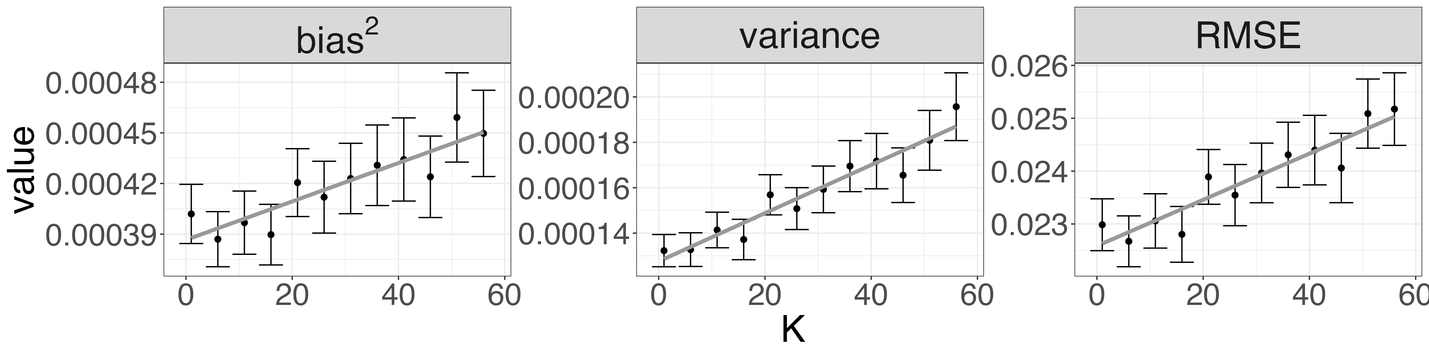
First, let to mimic the dataset of real American football plays. We compare the accuracy of an estimator fit from a dataset as the degree of dependence varies. The sample size in each of these datasets is (approximately) the same, . We visualize this bias-variance decomposition as varies in Figure 1. As the strength of the correlation increases, accuracy decreases linearly. In other words, fixing the number of observations in the dataset but increasing the degree of dependence across outcomes, which decreases the effective sample eize, reduces model accuracy. We compute the explicit reduction in effective sample size in the next Section 2.3.
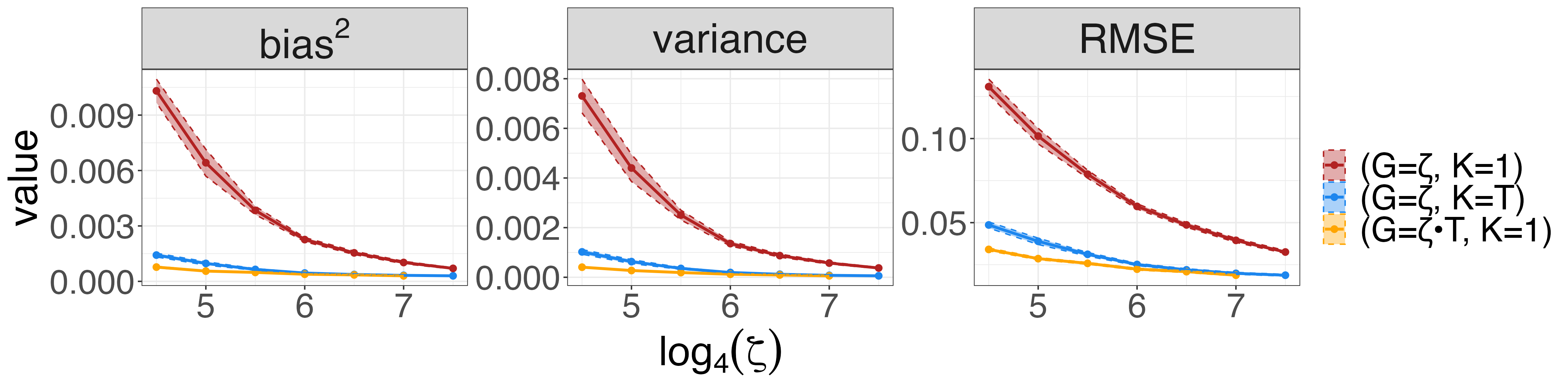
Next, as a function of sample size (with ), we compare the accuracy of estimators fit from three types of datasets. First, we consider a dataset, which involves keeping each generated play per game. This dataset mimics the historical dataset of real American football plays. Then, we consider a dataset, which keeps just one randomly sampled play per game. This dataset consists entirely of independent outcomes, and can be formed wholly from a dataset, but its sample size is much smaller ( rather than ). Finally, we consider a dataset, which has the same sample size (number of rows) as the first dataset, but consists entirely of independent outcomes.
In Figure 2 we visualize the bias-variance decomposition of win probability estimators fit from these three types of datasets as a function of . The -axis is because is the sample size of the historical dataset of American football plays. We see that it is much better to use all plays per game rather than one independent play per game. Despite the strong dependence structure, keeping all the plays provides information about the structure of the covariate space. We also see that it would be much better if the plays had independent outcomes. This suggests that the dependence structure reduces the effective sample size of the dataset. We explore the extent of this reduction in effective sample size in the next section.
2.3 Effective sample size
As discussed in the previous section, we can calculate the the accuracy of a win probability estimator fit from a dataset, denoted . The sample size (number of rows) of such a dataset with and , which mimics the historical dataset of American football plays, is . We saw that the dependence structure of this dataset reduces the accuracy of our estimator, but we’d like to understand the extent of this reduction. In particular, we are interested in the effective sample size () of that dataset. The is the sample size of a dataset consisting of independent outcomes, which produces an estimator having the same accuracy as one fit from the original dataset. For brevity, we refer to the sample size as and the effective sample size as , dropping the since we use throughout this study.
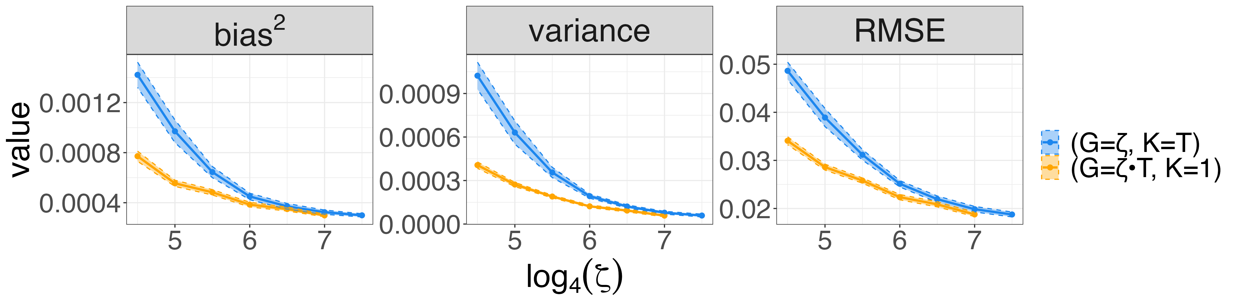
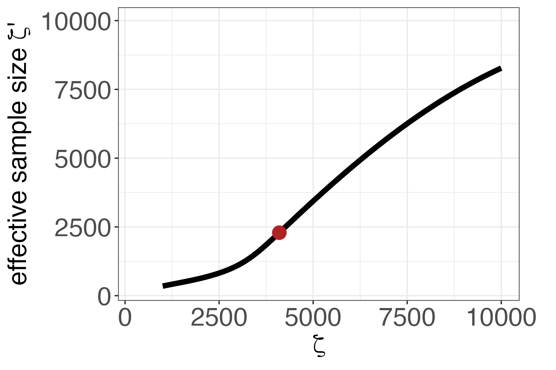
To estimate this effective sample size, we begin by fitting the and accuracy curves from Figure 2b. For each curve, we fit a biexponential model using nonlinear least squares. Then, as a function of , the effective sample size is the value satisfying . In Figure 3 we visualize the effective sample size as a function of . The effective sample size of a dataset is , or of the nominal sample size. This result is striking: we estimate that the historical dataset of American football plays (where ), consists of about half as much data as suggested by the number of plays. In other words, we are effectively fitting win probability from models years worth of independent win/loss outcomes, not years worth. Additionally, if we halved the size of our dataset, fitting a win probability model from games ( seasons) in order to, say, use just the most recent data, we estimate the effective sample size is , or just of the nominal sample size. If we doubled the size of our dataset, fitting a win probability model from games ( seasons), we estimate the effective sample size is , or of the nominal sample size.
2.4 Coverage of bootstrapped confidence intervals
We have seen that machine learning win probability models fit from noisy and highly correlated observational data are high variance estimators. Due to the dependence structure of historical football data, the effective sample size is much smaller than the nominal sample size. Therefore, it is critical to quantify uncertainty in win probability point estimates, as the point estimates alone may not be trustworthy. The bootstrap is a natural choice to capture such uncertainty since it is non-parametric and doesn’t make strong assumptions. Hence, in this section we explore the efficacy of bootstrapped win probability confidence intervals.
We begin with the standard (i.i.d.) bootstrap, which assumes each row (play) of the dataset is independently drawn. In the standard bootstrap, each of bootstrapped datasets are formed by re-sampling plays uniformly with replacement (recall is the number of games, is the number of plays per game, and is the total number of plays in a random walk football observational dataset). The standard bootstrap doesn’t match the dependence structure of our observational dataset. Hence, we also try the cluster bootstrap, in which each of bootstrapped datasets are formed by re-sampling games uniformly with replacement, keeping each observed play within each re-sampled game. Finally, in the randomized cluster bootstrap, each of bootstrapped datasets are formed by re-sampling games uniformly with replacement, and within each game re-sampling plays uniformly with replacement.
Each type of bootstrap produces bootstrapped datasets from the training dataset . We then fit a win probability model to each bootstrapped dataset using , . From these, we form a confidence interval for at game-state by the and quantiles of . Letting in this section, we form a confidence interval by . To avoid substantially low coverage near the extremes ( or ), we widen our confidence intervals when to have a lower bound of 0 and when to have an upper bound of 1.
We evaluate the efficacy of these bootstrapped confidence intervals by their coverage and width. For each type of bootstrap (standard bootstrap, cluster bootstrap, and randomized cluster bootstrap) and each simulation , we compute the pointwise marginal coverage of bootstrapped confidence intervals,
| (4) |
and the mean width,
| (5) |
We report the average of these values and the standard error in Table 1. To mimic the historical dataset of American football plays, each simulated dataset here consists of games, plays per game, and plays per game that share the same outcome.
| method | ||
| standard bootstrap | ||
| cluster bootstrap | ||
| randomized cluster bootstrap |
Even in our simplified setting of random walk football, each of these bootstrapped win probability confidence intervals are undercovered. The naive standard bootstrap in particular achieves dismally low marginal coverage. Even the randomized cluster bootstrap that accounts for the dependence structure doesn’t achieve high enough coverage. We suspect this coverage issue would be even worse for real American football, which is exponentially more complex than random walk football.
2.5 Calibrating bootstrapped confidence intervals
Since these naive bootstrapped confidence intervals are not wide enough, we wish to tune the bootstrap so that its nominally intervals indeed achieve marginal coverage. The traditional method of tuning non-parametric bootstrapped confidence intervals is to calibrate the bootstrapped quantiles (DiCiccio and Efron,, 1996). For instance, instead of using the and quantiles of to form a confidence interval, use the and quantiles for some .
In order for this traditional calibration method to work, would have to be much larger than , likely an order of magnitude larger (e.g., ). We, however, prefer to use lower values of (e.g., closer to ) than larger ones for several reasons. First, in order to develop applications that utilize bootstrapped win probability confidence intervals in real-time, such as fourth-down decision bots à la Brill et al., (2024), it is critical to keep small. Their fourth-down recommendations for one play take about 15 seconds when and about minutes when . The former can be run before a fourth-down play begins and the latter takes far too long. Additionally, storing machine learning models is much more expensive than storing of them. For these reasons, in this study we stray away from the traditional bootstrap calibration method.
Instead, we introduce a novel method to calibrate bootstrapped confidence intervals, the fractional bootstrap, that has the same time and storage complexity as traditional bootstrap methods. Specifically, we introduce a tuning parameter representing the fraction of data to be re-sampled in generating a bootstrapped dataset. By re-sampling less data than in the original dataset, we widen bootstrapped confidence intervals and increase coverage. In the fractional standard bootstrap, we re-sample plays (rows) uniformly with replacement. In the fractional cluster bootstrap, we re-sample games uniformly with replacement, keeping each observed play within each re-sampled game. Finally, in the fractional randomized cluster bootstrap, we re-sample games uniformly with replacement, and within each game re-sample plays uniformly with replacement.
In Table 2 we report the results of our simulation study in which we use to tune the randomized cluster bootstrap. To mimic the historical dataset of American football plays, each simulated dataset consists of games, plays per game, and plays per game that share the same outcome. As expected, lowering widens the confidence intervals and increases marginal coverage. In order for fractional randomized cluster bootstrapped confidence intervals to achieve nominal marginal coverage, needs to be as small as . Those intervals have a mean width of . This result is striking: in our simplified setting of random walk football, win probability confidence intervals need to be extremely wide to achieve nominal coverage. This exemplifies the difficulty of accurately estimating win probability by fitting a machine learning model from noisy and highly correlated football game outcomes. These are high variance estimators subject to large uncertainty.
| 1 | ||
| 0.75 | ||
| 0.5 | ||
| 0.35 |
Marginal coverage is a sufficient condition for confidence intervals to be “good,” but it is not a necessary condition. Even with marginal coverage, it could be that always covers for of game-states and never covers for the other of game-states . In that case, it may be disastrous to make decisions at the game-states for which intervals never cover. To check that our fractional randomized cluster bootstrapped confidence intervals achieve reasonable coverage across the space of game-states, we bin game-states by their true win probability and consider coverage in each bin. In Figure 4 we visualize coverage and its standard error across such bins. Although the intervals don’t achieve the nominal coverage in each bin, coverage is high enough in each bin for us to comfortably make decisions using these intervals.

References
- Baldwin, (2021) Baldwin, B. (2021). NFL win probability from scratch using xgboost in R.
- Brill et al., (2024) Brill, R. S., Yurko, R., and Wyner, A. J. (2024). Analytics, have some humility: a statistical view of fourth-down decision making.
- Carl and Baldwin, (2022) Carl, S. and Baldwin, B. (2022). nflfastR: Functions to Efficiently Access NFL Play by Play Data. https://www.nflfastr.com/.
- Chen and Guestrin, (2016) Chen, T. and Guestrin, C. (2016). XGBoost: A scalable tree boosting system. In Proceedings of the 22nd ACM SIGKDD International Conference on Knowledge Discovery and Data Mining, KDD ’16, pages 785–794, New York, NY, USA. ACM.
- DiCiccio and Efron, (1996) DiCiccio, T. J. and Efron, B. (1996). Bootstrap confidence intervals. Statistical Science, 11(3):189–212.
- Lock and Nettleton, (2014) Lock, D. and Nettleton, D. (2014). Using random forests to estimate win probability before each play of an nfl game. Journal of Quantitative Analysis in Sports, 10.
SUPPLEMENTARY MATERIAL
Appendix A Simulation study details
Formally, the outcome of the play of the game is
| (6) |
The game starts at midfield, , and the game begins tied, . The field position at the start of play is
| (7) |
and the score differential at the start of play is
| (8) |
The response column win is
| (9) |
As in our dataset of real football plays, this response column is highly correlated – plays from the same game share the same draw of the winner of the game.
The true win probability
| (10) |
of random walk football is computed explicitly using dynamic programming,
| (11) |
and
| (12) |