Interior convection regime, host star luminosity, and predicted atmospheric CO2 abundance in terrestrial exoplanets

Abstract

Terrestrial planets in the Habitable Zone of Sun-like stars are priority targets for detection and observation by the next generation of powerful space telescopes. Earth’s long-term habitability may have been tied to the geological carbon cycle, a process critically facilitated by plate tectonics. In the modern Earth, plate motion corresponds to a mantle convection regime called mobile-lid. The alternate, stagnant-lid regime is found on Mars and Venus, which may have lacked strong enough weathering feedbacks to sustain surface liquid water over geological timescales if initially present. Constraining observational strategies able to infer the most common regime in terrestrial exoplanets requires quantitative predictions of the atmospheric composition of planets in either regime. We use endmember models of volcanic outgassing and crust weathering for the stagnant- and mobile-lid convection regimes, that we couple to models of atmospheric chemistry and climate, and ocean chemistry to simulate the atmospheric evolution of these worlds in the Habitable Zone. In our simulations under the two alternate regimes, we find that the fraction of planets possessing climates consistent with surface liquid water differ by less than 10%. Despite this unexpectedly small difference, we predict that a mission capable of detecting atmospheric CO2 abundance above 0.01 bar in 25 terrestrial exoplanets is extremely likely ($\geq 95$% of samples) to infer the dominant interior convection regime in that sample with strong evidence (10:1 odds). This offers guidance for the specifications of the Habitable Worlds Observatory NASA concept mission and other future missions capable of probing samples of habitable exoplanets.

1 Introduction

The question of whether Earth’s habitability is generic or specific among rocky planets in the Habitable Zone (HZ, the range of orbital radii as a function of stellar mass for which rocky planets with surface liquid water do not undergo greenhouse nor global glaciation runaway; Huang, 1959; Hart, 1979; Kasting et al., 1993; Kopparapu et al., 2013) is central to the search for extraterrestrial life. Planets of composition and size similar to the Earth’s –terrestrial exoplanets– in the HZ of Sun-like (FGK-type stars) have not yet been observed and thus are priority targets for detection and characterization by the next generation of ground-based and space telescopes (National Academies of Sciences, Engineering, and Medicine, 2021). Exoplanet atmospheric compositions inferred from such observations may serve to confirm or reject that these planets are habitable in the sense that liquid water is actually present on their surface (Robinson, 2018; Cockell et al., 2016).

These analyses, however, are likely to come with large degrees of uncertainty and ambiguity. To alleviate such ambiguity, three steps can be taken. First, atmospheric exoplanet data should be interpreted given the planet’s context by taking into account planetary characteristics such as orbit radius, host star mass, planet radius, mass, age, and formation pathways (Meadows et al., 2018; Apai et al., 2018; Bixel & Apai, 2020; Krissansen-Totton et al., 2022). Second, Bayesian inference makes it possible to combine contextual information, used to shape prior distributions, with observations, to derive posterior probabilities of habitability and inhabitation (Catling et al., 2018a). Finally, the assessment of habitability and putative inhabitation will be more robust by analyzing patterns of atmospheric composition across a sample of exoplanets, rather than the detailed characterization of any single planet (Bean et al., 2017; Bixel & Apai, 2021; Mazevet et al., 2023). In recent years, there has been some pioneering effort to implement this agenda (e.g. Lehmer et al., 2020; Bixel & Apai, 2020). Yet we are still lacking predictions of population-level atmospheric patterns of habitability and potential for life emergence under alternate geophysical hypotheses, and a quantitative evaluation of their testability.

The HZ framework typically provides limit values of luminosity above and below which no surface liquid water is expected (Kopparapu et al., 2013; Kasting et al., 1993). However, these analyses cannot predict how likely the presence of surface liquid water is on planets within the HZ boundaries. Constraining the climate of the Earth in the distant geological past is difficult. Krissansen-Totton & Catling (2017) used a parametric model of the geological carbon cycle (Kasting, 1993) and climate to show that the evolution of atmospheric CO2 as estimated from fossil weathering profiles (Rye et al., 1995; Hessler et al., 2004; Sheldon, 2006; Kanzaki & Murakami, 2015) is consistent with the persistence of a relatively temperate climate as the Sun became increasingly bright. Drawing a parallel between the changing luminosity of the Sun and varying orbital radii around a star of constant brightness, it is commonly hypothesized that geophysical processes assumed to have stabilized the Earth’s climate –the geological carbon cycle– would ensure that planets within the HZ have climates compatible with surface liquid water (Kasting et al., 1993; Catling et al., 2018b). In other words, the concept of the HZ as currently defined rests largely on the hypothesis of the geological carbon cycle as a global negative feedback loop to climate.

Lehmer et al. (2020) proposed testing the hypothesis that an Earth-like geological carbon cycle acts as a planetary thermostat that ensures temperate climates across the range of incident stellar light flux in the HZ. Their model of the Earth’s geological carbon cycle predicts a correlation between luminosity and atmospheric pCO2. In their simulations, sampling about 83 exoplanets is required to reject the null hypothesis of a log-uniform (uncorrelated) distribution, a number far greater than the target yield of the NASA Flagship concept Habitable Worlds Observatory (Mamajek & Stapelfeldt, 2023).

While this work provides an important first step, its calculation of the false negative decision risk (frequency of non rejection of the assumed false null hypothesis) relies on an ad hoc null hypothesis with no explicit geophysical basis. Even in the absence of a geological carbon cycle, photochemical reactions in the atmosphere may affect the abundance of CO2 over geological timescales. In addition, continental weathering relies primarily on continental crust minerals (silicates and carbonates) being exposed to precipitations. The accretion of continental crust is dependent upon plate tectonics, a process that our planetary neighbors Mars and Venus do not appear to have or have had (Solomatov & Moresi, 1996; Catling & Kasting, 2017), and that may have had a late onset on Earth (although this view is being challenged; see Windley et al., 2021). No planet in our solar system appears to have been in any one clearly defined interior convection regime during the entirety of its geological history. However, it appears that two distinct end-member scenarios that are relevant to a planet’s habitability can be drawn: That the potential habitability of terrestrial planets be supported by the geological carbon cycle as enabled by Earth-like plate tectonics equated with the ”mobile-lid” (ML) interior convection regime; or as an alternate hypothesis that terrestrial planets in general remain in the ”stagnant-lid” (SL; also referred to as single-lid) interior convection regime, in which no crust recycling or continental crust accretion occur (Figure 1A).

It is often assumed that for conditions favorable to surface habitability, in particular a temperate climate persisting on geological timescales, weathering of continental rocks (silicates and carbonates; ’continental weathering’) is required (Catling & Kasting, 2017). This assumption, in combination with Earth’s unique interior convection regime among terrestrial planets in the solar system, may lead to expect that most terrestrial planets orbiting in the habitable zone of other stars may not effectively possess surface liquid water. However, weathering of non-continental emerged land may still participate to the geological carbon cycle, and the seafloor dissolution of basalt can also drive a negative feedback to atmospheric CO2 that does not hinge on the existence of continental crust (see Figure 1B, and Krissansen-Totton et al., 2018; Gillis & Coogan, 2011). Seafloor weathering may allow terrestrial planets with a limited supply of subaerial weatherable silicates and carbonates to retain a geological carbon cycle as a negative feedback loop to climate (Lenardic et al., 2016), albeit a possibly weaker one (Sleep & Zahnle, 2001). Planets in the SL regime are assumed to have a shorter-lived period of volcanic outgassing due to the absence of recycling of crust-bound CO2 and the thickening of the lithosphere as the mantle cools (Figure 1C; Dorn et al., 2018). Nevertheless, early on they may support an ocean and sufficient basalt production to sustain controlled atmospheric CO2 through seafloor weathering. Thus, even though continental weathering conservatively remains the main process for long-term Earth-like habitability, the findings of first-order analyses of planets atmosphere in the SL regime call for models that fully couple interior, ocean, and atmospheric processes to evaluate the habitability of SL worlds (Foley & Smye, 2018; Foley, 2019; Tosi et al., 2017).

How likely terrestrial planets in the HZ might be and remain habitable, or even possibly host life, could thus largely depend on the influence of a convection regime on climate, and on what convection regime is the most common. Under the seemingly pessimistic assumption that terrestrial exoplanets in the HZ are in the SL regime, how likely are they to possess stable temperate climates? What are the key planetary parameters that this depends on? And how can this inform the design of future exoplanet survey missions to assess how widespread SL and ML interior convection regimes are, at minimal cost? To answer these questions, we present an integrated model in which atmospheric photochemistry is coupled with ocean chemistry, weathering processes, and climate. We model equilibrium atmospheric composition in the two concurrent interior convection regime by adopting endmember models for relating volcanic outgassing to planetary age (Krissansen-Totton et al., 2018; Dorn et al., 2018), and set the weathering of sub-aerial rocks to be zero in the SL regime. Models for the evolution of outgassing rate on Earth-sized planets remain scarce and large uncertainties are associated with them, especially in the case of the stagnant-lid regime. Given these uncertainties, we focus on a nominal model for Earth’s history for the ML convection regime (Krissansen-Totton et al., 2018), and the model outputs from Dorn et al. (2018) for the SL convection regime. The coupled model offers a significant step towards the generalization of early-Earth models that include the biological activity of microbial biospheres (Sauterey et al., 2020). The model also extends previous work in which photochemistry as well as outgassed greenhouse gases other than CO2, such as methane or dihydrogen, were omitted (Lehmer et al., 2020; Foley & Smye, 2018). By feeding simulations of our model into a Bayes factor based experimental design analysis, we predict which combination of minimally detectable CO2 and sample size offers the highest chance of inferring the dominant interior convection regime with sufficient evidence.

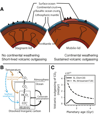
Figure 1: Key geophysical and geochemical processes of stagnant-lid (SL) and mobile-lid (ML) convection regimes in the interior-ocean-atmosphere coupled model. A Key geophysical processes. The dashed curves in the mantle represent isotherms highlighting convective plumes. B Key geochemical processes and their influence of global temperature. Brown and blue arrows indicate the contribution of continental (brown arrows) and seafloor (blue arrows) to the climate-stabilizing negative feedback. Triangle-headed arrows indicate positive effects (increase in quantity), whereas flat-headed arrows indicate negative effects (removal or decrease). Two-ways arrows represent dissolution or chemical equilibrium. Brown arrows correspond to processes exclusive to the silicate-carbonate feedback. Dotted blue arrows correspond to processes exclusive to the basalt dissolution (seafloor weathering) feedback. C CO2 volcanic outgassing rate as a function of planetary age as proposed for the Earth, that we use as the ML regime nominal model (dashed curve; KrissansenT18 indicates model from Krissansen-Totton et al., 2018) and for one Earth mass SL planets (continuous curve; Dorn18 indicates model from Dorn et al., 2018)

2 Methods

Our goal is to simulate the atmospheric composition and habitability of terrestrial exoplanets under various conditions of luminosity and for two regimes of interior convection: the stagnant-lid (SL) and the mobile-lid (ML) regimes. To do so, we couple slightly modified versions of models describing the influence on atmospheric composition of ocean and atmospheric chemistry, as well as chemical exchanges between the atmosphere and the crust, the ocean and the atmosphere, and the crust and the ocean (Arney et al., 2016; Krissansen-Totton & Catling, 2017). Thus, we generalize existing coupled models beyond the particular case of the Archean Earth (Kharecha et al., 2005; Sauterey et al., 2020). In this section, we present the description of each of these models and their assemblage into our coupled model. Then, simulations resulting from this coupled model are used to perform statistical analyses that project the potential yield of future observational strategies as described in Results Section Simulated inference of dominant interior convective regime among terrestrial exoplanets.

First, we describe how our coupled model is built. We expand on models designed for simulating the climate of the Archean Earth (Sauterey et al., 2020; Krissansen-Totton et al., 2018; Kharecha et al., 2005). We select a restricted number of molecules of which the abundance in the atmosphere is modeled. These are chosen for their importance in determining the planet’s surface temperature (loosely referred to as climate throughout the text) and thus potential habitability, their participation to geochemical processes relevant to climate, and their potential use for an early biosphere similar to Earth’s early biosphere (Sauterey et al., 2020):H2, CO2, CH4, and CO.

Several key planetary parameters could affect the equilibrium value of the abundance of those gases in the atmosphere of a terrestrial planet. Volcanic outgassing ($F_{out}$, mol yr^-1), taken broadly, releases most of those molecules (and others) into the atmosphere, has played a key role in setting the climate of the early Earth (and still does so today), and has changed over geological times on Earth (Krissansen-Totton et al., 2018). It is also believed that volcanic outgassing may vary in its intensity depending on the interior convection regime a planet is exhibiting. Second, the quantity of light (luminosity) a planet receives from its star is expected to be a first-order determining factor of its climate (its value relative to that of the modern Earth is noted $S/S_{\earth}$). Last, weathering cycles that participate to set atmospheric CO2 require that fresh weatherable minerals are exposed to the planetary surface, hence it depends on volcanic activity on the one hand, and on the surface of crust that is exposed to precipitations, denoted by the fraction of the planetary surface $f_{land}$. Together, these parameters compose the vector $\boldsymbol{\theta}=(F_{out},S/S_{\earth},f_{land})$. Other than for those parameters, it is assumed that the simulated planet is identical to the Earth (one Earth mass, 1 bar atmosphere).

Ultimately, we aim at building a system of differential equations that describes the rate of change of the vector composed of partial pressures in the atmosphere $\boldsymbol{y}=(p\ch{H2},p\ch{CO2},p\ch{CH4},p\ch{CO})$ as a function $\mathrm{F}$ of $\boldsymbol{y}$ itself and the parameters $\boldsymbol{\theta}$:

$$\dot{\boldsymbol{y}}=\mathrm{F}_{\boldsymbol{\theta}}(\boldsymbol{y})~{}.\\$$ (1)

If the geological timescale (on which $\boldsymbol{\theta}$ changes) is much slower than the climate timescale (on which $\boldsymbol{y}$ changes), the system of differential equations in Equation (1) is seen as autonomous, i.e. the function $\mathrm{F}$ does not explicitly depend on time $t$. In the following sections, we develop the components of the function $\mathrm{F}_{\boldsymbol{\theta}}(\boldsymbol{y})$ that involve atmospheric photochemistry (Methods Section Atmospheric photochemistry and climate), exchanges between the ocean and the atmosphere (Methods Section Molecular flux across the ocean/atmosphere interface), and ocean chemistry of carbonates and carbon monoxide including its relation to geochemical processes such as weathering (Methods Section Ocean-Atmosphere coupling).

2.1 Atmospheric photochemistry and climate

Our goal is to derive a numerical method to obtain the rate of change of atmospheric mixing ratios due to a set photochemical reactions denoted $\boldsymbol{\Phi}$ (molecules cm^-2 s^-1), the surface temperature $T_{s}$ (K), and the planetary albedo ($A_{P}$) given the atmospheric mixing ratios $\boldsymbol{y}$ (in Pa):

$$(\boldsymbol{\Phi},T_{s},A_{P})=\mathrm{F}^{atm}_{\boldsymbol{\theta}}(\boldsymbol{y})~{}.\\$$ (2)

Studies that aim to determine the boundaries of the Habitable Zone (HZ) adopt an inverse modeling approach where outgoing longwave radiation is calculated for various temperatures (Kasting et al., 1993; Kopparapu et al., 2013). However, we aim to roughly calculate climatic conditions and atmospheric composition of terrestrial planets that lie within the HZ by assumption. This introduces a number of differences in the way atmospheric modeling is handled in our coupled model, which are detailed in this section.

We use Atmos, a 1-D coupled photochemistry and climate model (Arney et al., 2016), that we run over ranges of values for (pH2, pCO2, pCH4,$S/S_{\earth}$). Then, the output simulations are interpolated to create a numerical function which approximates $\mathrm{F}_{\boldsymbol{\theta}}^{atm}$ in Equation (2). The Atmos model simulates the equilibrium vertical profile (with respect to photochemistry and climate) of the abundance of molecules in the atmosphere given a set of boundary conditions that are either (i) fixed molecular fluxes or (ii) fixed gas mixing ratios at the bottom-most layer of the discretized atmosphere. Using boundary conditions defined as fixed deposition or outgassing rates instead of fixed molecular abundances would lead the model to calculate the vertical composition of the atmosphere at the equilibrium between the imposed surface fluxes and photochemical reactions. This would then lead to a discrepancy between the state of the atmosphere calculated by the photochemical model and the out-of-equilibrium atmospheric composition that is used to calculate geochemical fluxes (weathering and ocean/atmosphere exchanges) that constitutes the set of dynamic variables of the model $\boldsymbol{y}$ (Equation 1). In order to use this model to obtain photochemical rates when the lower atmosphere has a composition given by vector $\boldsymbol{y}$, we need to run it using defining boundary conditions as fixed mixing ratios $\boldsymbol{y}=(p\ch{H2},p\ch{CO2},p\ch{CH4},p\ch{CO})$.

We thus use Atmos with fixed molecular abundances in the lowest atmospheric layer as boundary conditions for H2, CO2, and CH4. We need to run the photochemical model under various values of these boundary conditions (and of luminosity) to simulate atmospheric evolution coupled with other processes. This is computationally demanding, hence apart from H2, CO2, and CH4, we set the boundary conditions for other gases to be the default fixed surface fluxes (Earth-like values) already set in Atmos such that they are not dynamic variables in our coupled model. For carbon monoxide (CO), which is a dynamic variable of our coupled model through the modeling of its ocean chemistry (Methods Section Ocean-Atmosphere coupling), we still use a constant boundary condition in Atmos that is a surface deposition flux $v_{dep}=1.2\times 10^{-4}$ cm s^-1 (Kharecha et al., 2005). This value for the deposition velocity of CO is the default in Atmos and corresponds to estimates based on the consumption of $\ch{CO}$ by organisms in the ocean, and is expected to be up to four orders of magnitude higher than abiotic estimates (Kharecha et al., 2005; Sauterey et al., 2020). Our model does not otherwise include any participation of biogenic fluxes to geochemical cycles. Intuitively, this would lead to overestimate the rate of the CO-producing reactions, and underestimate that of CO-consuming reactions in the atmosphere, since imposing a higher sink of CO at the surface forces equilibrium photochemical rates to produce more CO than they would in a hypothetical case with only abiotic sinks. In the atmosphere of the Archean Earth, CO is produced by photolysis of CO2 (Sauterey et al., 2020, and references therein), but CO can also react with water to form CO2 (among other molecules; Bar‐Nun & Chang, 1983). This leads to non-trivial interactions between CO and CO2 in our model, which do not appear in other models (Sauterey et al., 2020; Kharecha et al., 2005). Typical photochemical sources or sinks of carbon dioxide are found to be at most of the order of $10^{4}-10^{6}$ mol yr^-1 (Figure 2A), several orders of magnitude lower than typical values of volcanic outgassing or of weathering rates (up to the order of $10^{13}$ mol yr^-1; Krissansen-Totton et al., 2018, and Figure 1C). Comparison between our model interpolation and the parameterization in the early-Earth model in Sauterey et al. (2020) (which is based on the 1D version of the generic LMD global circulation model) reveals that the photochemical sink of CO2 in our model is lower by a factor 2. At low CO2 pressures ($\approx 10^{-4}$ bar), our model predicts a CO2 source in atmospheric photochemistry (Figure 2A), which is not predicted by the parameterization by Sauterey et al. (2020). Thus, the particular value of the CO deposition velocity is of negligible impact in our study. However, future implementations of this model that may include CO producing or consuming microbes should use atmospheric abundance boundary condition for this gas, as we do for CO2, H2, and CH4.

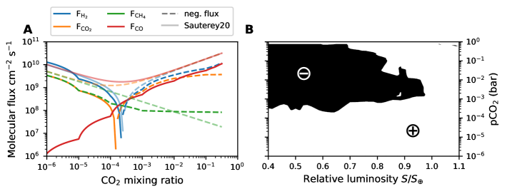
Figure 2: A Photochemical rates of production (solid lines) and alteration (dashed lines) of molecules included in our coupled model calculated from our interpolation of Atmos outputs or calculated from the parameterization in Sauterey et al. (2020) (semi-transparent lines). These calculations assume $S/S_{\earth}=0.8$, the value of the luminosity assumed for the Archean Earth in the parameterization of Sauterey et al. (2020). Other gases are fixed at p$\ch{CH4}=0.1$ ppm and p$\ch{H2}=100$ ppm, average values in our simulations. B Sign of the photochemical flux of CO2 as a function of atmospheric concentration in CO2 and relative luminosity. Dark areas represent pCO2-luminosity conditions in which the photochemistry results in net removal of CO2, and the white region of the plot represent conditions in which photochemistry results in net production of CO2. These calculations use fixed p$\ch{CH4}=0.115$ ppm and p$\ch{H2}=35$ ppm, average values in simulations in the SL regime that have final p$\ch{CO2}>10^{-3}$ bar.

We ran 6312 simulations of the coupled photochemistry-climate model for boundary conditions in the lower atmosphere varying from $10^{-8}$ to $10^{-1}$ bars of $\ch{H2}$, $\ch{CH4}$ and from $10^{-8}$ to $0.8$ bars for $\ch{CO2}$ (Figure 3) and with a relative luminosity $S/S_{\oplus}$ varying from $0.4$ to $1.4$, corresponding to orbital distances from the Sun comprised between $0.85$ and $1.58$ au. Such a grid is bound to include simulations that do not correspond to an equilibrium in the vertical profile of atmospheric composition, or that correspond to climate regimes beyond the scope of this analysis (e.g., organic hazes or runaways). Such cases are thus discarded from our set of simulations used to model atmospheric evolution on geological timescales.

Figure 3: Climate calculations in the $p\ch{CO2}$ versus $p\ch{CH4}$ space for $S/S_{\oplus}=0.8$ and $p\ch{H2}=10^{-5}$ bar. The dots represent simulations made with the photochemistry/climate coupled model, and their color reflects the calculated surface temperature at radiative equilibrium.

The atmospheric model assumes a total pressure of 1 bar in the atmosphere, completed with $\ch{N2}$. However, the dynamics of the model do not guarantee that an equilibrium is found with an atmosphere of only 1 bar, hence we halt and discard simulations that reach $p\ch{H2}+p\ch{CH4}+p\ch{CO2}\geq 1$ bar. It is expected that organic hazes start forming when the $\ch{CH4}:\ch{CO2}$ ratio exceeds unity (Zahnle, 1986; Kharecha et al., 2005). These hazes might have an anti-greenhouse climatic effect that we do not account for in our version of Atmos in order to save computation time. Hence, simulations in which $p\ch{CH4}\geq p\ch{CO2}$ are discarded (Figure 3).

Ultimately, 4806 climate and photochemistry simulations that have successfully converged are retained and used in the general coupled model. As shown later, some simulations of the dynamical evolution of the atmospheric composition may reach the border of the 4-D volume in which the atmosphere is modeled. In such cases, the simulations are halted.

It is important to note here that we assumed the same type of vertical profile of water vapor across the entire range of our atmospheric photochemistry and climate simulations. The vertical profile of water that we used to initialize the climate-photochemistry simulations is described by Manabe & Wetherald (1967), and assumes a non water-saturated troposphere. This water vapor vertical profile matches empirical expectations for the atmosphere of the modern Earth (Catling & Kasting, 2017). It is unknown whether such a profile is more or less realistic than assuming a water-saturated troposphere as commonly done to infer the water loss limit (Kopparapu et al., 2013). In consequence, our simulations may underestimate the surface temperature of planets that are closer to the inner edge of the HZ, thus deviating from results of Kopparapu et al. (2013), as shown in Figure 4A. Furthermore, our assumption of a 1 bar atmosphere prevents modeling $\ch{CO2}$-rich dense atmospheres ($>1$ bar) that could remain temperate at relative luminosity values as low as $S/S_{\oplus}=0.34$ (Kopparapu et al., 2013). Further exploration of changes in water saturation is beyond the scope of this first study, but future work should allocate effort into relaxing that assumption.

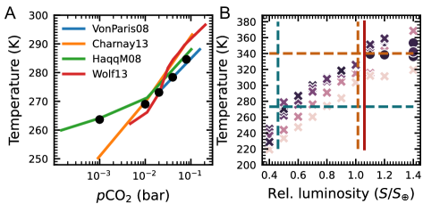
Figure 4: A Comparison of habitable zone results. The simulations are represented as crosses when they have converged and circles when they have not. In the cases that did not converge, the temperature retained and plotted is representative (the last recorded iteration of the climate simulation), but does not correspond to an atmosphere in radiative equilibrium. The color code of the simulations is shown in the legend and corresponds to the partial pressure of $\ch{CO2}$ forced constant at the bottom of the atmosphere. The blue dashed lines correspond to the outer edge of the HZ. The horizontal one is set at $T=0$°C, and the vertical one is set at the OHZ $S/S_{\oplus}=0.46$ value calculated in Kopparapu et al. (2013) for pCO2=1 bar. The orange dashed lines represent the IHZ: horizontally at the surface temperature $T_{S}=340$ K at which the moist greenhouse or water loss limit is reached (Methods Section Atmospheric photochemistry and climate), and vertically at the consensus luminosity at which this limit is reached $S/S_{\oplus}=1.015$ (Kopparapu et al., 2013). The solid red vertical line corresponds to the greenhouse runaway limit $S/S_{\oplus}=1.06$ (Kopparapu et al., 2013). B Comparison of climate simulations from the Atmos model used here (black circles) and previously published simulations for an early Earth at $S/S_{\oplus}=0.8$ (approximately 2.8 billion years ago, Charnay et al., 2013; Wolf & Toon, 2013; Haqq-Misra et al., 2008; von Paris et al., 2008). These calculations assume fixed abundances pH2=100ppm, and pCH4=0.1ppm, which are the average values in our simulations with age $\tau\in[2,3]$ Gyrs and $S/S_{\earth}\in[0.75,0.85]$.

Within the radiative equilibrium regime, we observe that the temperatures calculated in our climate simulations are in relatively good agreement with previously published results (Figure 4B). 1D models appear to overestimate the warming effect of low partial pressures of $\ch{CO2}$, and underestimate it at higher abundances. These differences are well documented (Fauchez et al., 2021). Three-dimensional Global Climate Models (GCMs) are expected to constitute a reference, and the differences mentioned above are to be kept in mind when interpreting the results of our simulations relying on the Atmos climate model (see Fauchez et al., 2021, for a comprehensive comparison between different atmosphere models).

In order to use the climate and photochemical calculations to integrate the set of differential equations summarized by Equation (1), the result of atmospheric simulations are interpolated (using the linear ND interpolator from SciPy; Virtanen et al., 2020) in the 4-D space comprising the grid (utilizing the $\log_{10}$ of partial pressures) in order to obtain the following continuous functions:

$$\begin{array}[]{rcl}(T_{S},A_{P})&=&F_{1}(p\ch{H2},p\ch{CO2},p\ch{CH4},S/S_{\oplus})\\ (\Phi_{\ch{H2}},\Phi_{\ch{CO2}},\Phi_{\ch{CH4}},\Phi_{\ch{CO}})&=&F_{2}(p\ch{H2},p\ch{CO2},p\ch{CH4},S/S_{\oplus})\end{array}$$ (3)

where $T_{S}$ (K) is the surface temperature, and $A_{P}$ the planetary albedo. $\Phi_{i}$ (molecules cm^-2 s^-1) are photochemical fluxes.

2.2 Ocean-Atmosphere coupling

Next, atmospheric composition is influenced by the exchange of gases across the ocean’s surface. Previous models implicitly assume that the ocean and the atmosphere are at solubility equilibrium, i.e. that the concentration of molecule $\ch{X}_{i}$ in the ocean follows Henry’s law $[\ch{X}_{i}]=\alpha_{\ch{X_{i}}}p\ch{X_{i}}$, with $\alpha_{\ch{X_{i}}}$ ($\text{mol}~{}\text{L}^{-1}~{}\text{bar}^{-1}$) the Henry coefficient for $\ch{X_{i}}$, and $p\ch{X_{i}}$ the gas partial pressure of $\ch{X_{i}}$ in the atmosphere (bar; e.g. Krissansen-Totton et al., 2018). Instead of assuming thermodynamic equilibrium between the ocean and the atmosphere, we explicitly describe the dynamics of the concentrations of relevant molecules in the ocean governed by subaquatic volcanic outgassing, and carbonate precipitation and dissolution. These dynamics include a net flux to or from the atmosphere due to the ocean and atmosphere not being at thermodynamic equilibrium. We then calculate the steady-state of the ocean’s composition by assuming that the atmospheric composition remains constant on the timescale over which this equilibrium is reached. As a result, we obtain the flux across the ocean/atmosphere interface as a function of atmospheric composition.

2.2.1 Molecular flux across the ocean/atmosphere interface

The exchange rate between the ocean and the atmosphere is described by Equation (4), corresponding to the stagnant boundary layer (SBL) model (Kharecha et al., 2005):

$$\mathrm{F}_{oc}(\ch{X_{i}})=v_{\ch{X_{i}}}(\ch{[X_{i}]}-\alpha_{\ch{X_{i}}}p\ch{X_{i}})\times C$$ (4)

where $\mathrm{F}_{oc}$ ($\text{molecules}~{}\text{cm}^{-2}~{}\text{s}^{-1}$) is the flux of molecule $\ch{X}_{i}$ across the atmosphere-ocean interface (counted positive for flux to the atmosphere) for the chemical species $\ch{X}_{i}$, $v_{\ch{X}_{i}}$ is a piston velocity across the stagnant boundary layer ($\text{cm}~{}\text{s}^{-1}$, for a $40~{}\mu\text{m}$ thick SBL), $\alpha_{\ch{X}_{i}}$ is the Henry coefficient ($\text{mol}~{}\text{L}^{-1}~{}\text{bar}^{-1}$), $p\ch{X}_{i}$ is the gas partial pressure in the atmosphere (bar), $[\ch{X}_{i}]$ is the concentration of $\ch{X}_{i}$ in the ocean ($\text{mol}~{}\text{L}^{-1}$) and $C=\mathrm{A}/10^{3}~{}\text{molecules}~{}\text{mol}^{-1}/(\text{cm}^{3}~{}\text{L}^{-1})$ with $\mathrm{A}=6.02\times 10^{23}$ mol^-1 the Avogadro number.

To track concentration change in the ocean, it is more useful to rearrange some elements of Equation (4) into a diffusion constant

$$D_{\ch{X_{i}}}=\frac{v_{\ch{X_{i}}}}{z_{oc}}~{}(\text{s}^{-1})$$ (5)

where $z_{oc}$ is the ocean depth (in cm). The volume of the ocean is set constant using $M_{o}=3\times 10^{21}$ kg and $\rho_{oc}=1000$ kg m^-3 in all our simulations. However, the ocean surface is not set constant, as we allow variable emerged land surface. Thus, the depth of the ocean $z_{oc}$ is calculated using

$$z_{oc}=\frac{V_{oc}}{S_{p}(1-f_{land})}$$ (6)

where $S_{p}=5.1\times 10^{18}$ cm^-2 is the total surface of the planet, and $f_{land}$ is the fraction of the surface of emerged land (not necessarily continental crust) so that the ocean surface $S_{oc}=(1-f_{land})S$. Last, $\mathrm{F}_{oc}$ ($\text{molecules}~{}\text{cm}^{-2}~{}\text{s}^{-1}$) is converted into $\mathrm{F}_{oc}^{\prime}$ (mol yr^-1):

$$\mathrm{F}_{oc}^{\prime}=D_{\ch{X}_{i}}(\alpha_{\ch{X}_{i}}p\ch{X_{i}}-[\ch{X}_{i}])\times(3600\times 24\times 365.25)~{}.$$ (7)

2.2.2 Carbon monoxide ocean chemistry

Following the Appendix 3 of Kharecha et al. (2005), we parameterize the kinetics of the photochemical conversion, in the upper ocean, of CO to formate (HCOO-) and subsequently to acetate following

$$\ch{CO}+\ch{OH-}\xrightleftharpoons[k_{2}]{k_{hyd}}\ch{HCOO-}(+\cdots)\xrightarrow{k_{3}}\ch{CH3COO-}(+\cdots).$$ (8)

The steady-state of these reactions (equation 8) coupled with the rate of exchange with the atmosphere (equation 7) results leads to

$$\begin{array}[]{r c l}[\ch{CO}]&=&\frac{\alpha_{\ch{CO}}p\ch{CO}D_{\ch{CO}}(k_{2}+k_{3})}{k_{3}k_{hyd}[\ch{OH-}]+(k_{2}+k_{3})D_{\ch{CO}}}\\ [\ch{HCOO-}]&=&\frac{\alpha_{\ch{CO}}p\ch{CO}D_{\ch{CO}}k_{hyd}[\ch{OH-}]}{k_{3}k_{hyd}[\ch{OH-}]+(k2+k3)D_{\ch{CO}}}\end{array}$$ (9)

where $[\ch{OH-}]$ is derived from the pH (variable in our model) and the ionic product of water in standard conditions $\ch{pK_{e}}=\ch{pH}+\ch{pOH}=14$.

2.2.3 Carbon cycle in a coupled ocean-atmosphere model

Continental weathering transfers atmospheric (and crustal) carbon to the ocean. This occurs as the products of the weathering of continental crust minerals are transported in rivers:

$$\begin{array}[]{rcl}\ch{CO_{2}}+\ch{H_{2}O}+\ch{CaCO_{3}}&\longrightarrow&\ch{Ca^{2+}}+2\ch{HCO_{3}^{-}}\\ 2\ch{CO_{2}}+\ch{H_{2}O}+\ch{CaSiO_{3}}&\longrightarrow&\ch{Ca^{2+}}+2\ch{HCO_{3}^{-}}+\ch{SiO_{2}}.\end{array}$$ (10)

Then, carbonates can precipitate in the ocean (at a pH-dependent rate noted $P_{o}$ in mol yr^-1; equation 11), of which a certain fraction returns to the crustal reservoir through diagenesis

$$\ch{Ca^{2+}}+2\ch{HCO_{3}^{-}}\longrightarrow\ch{CO_{2}}+\ch{H_{2}O}+\ch{CaCO_{3}}.$$ (11)

The rate of the reactions in Equation (10) are assumed to have increased with the global mean surface temperature of the Earth, hence providing a negative feedback loop on climate through the abundance of atmospheric carbon (Figure 1B; Walker et al., 1981; Krissansen-Totton & Catling, 2017). It has been assumed that other terrestrial planets could undergo similar climate stabilization. This is used to explain the inner edge of the HZ being set by the greenhouse effect of water vapor, and that the maximum partial pressure of CO2 (before condensation) setting the traditional outer edge of the HZ (Kasting et al., 1993; Kopparapu et al., 2013).

A second temperature-sensitive process that can transfer atmospheric carbon to the crustal reservoir is seafloor weathering (Krissansen-Totton & Catling, 2017; Gillis & Coogan, 2011; Alt & Teagle, 1999). This process does not rely on the alteration of continental crust, but rather on the dissolution of the basaltic seafloor occurring at off-axis hydrothermal circulation, releasing cations such as Ca^2+ hence promoting reaction 11 (by increasing $[\ch{Ca^{2}+}]$ and carbonate alkalinity through ionic balance; see Figure 1B).

We largely reproduce the model of carbonate chemistry and the carbonate-silicate weathering cycle in Krissansen-Totton & Catling (2017) with only slight modifications to allow the bulk ocean and the atmosphere to be in disequilibrium (unlike Krissansen-Totton & Catling, 2017; Lehmer et al., 2020, where the ocean and atmosphere are treated as at equilibrium).

Following Krissansen-Totton & Catling (2017) we track the concentration of dissolved carbon (DIC) and carbonate alkalinity (ALK; both defined in Equation 12) in the upper and deep ocean that mix at constant rate $J=6.8\times 10^{16}$ kg yr^-1.

$$\begin{array}[]{rcl}\ch{DIC}&=&\ch{[CO_{2}]_{aq}}+\ch{[HCO_{3}^{-}]}+\ch{[CO_{3}^{2-}]}\\ \ch{ALK}&=&\ch{[HCO_{3}^{-}]}+2\ch{[CO_{3}^{2-}]}.\end{array}$$ (12)

The overall dynamics of the carbonate system in the ocean (subscript $o$) and deep ocean (subscript $d$) follows:

$$\begin{array}[]{r c l}\dfrac{\mathrm{d}C_{o}}{\mathrm{d}t}&=&\overbrace{D_{\ch{CO2}}(\alpha_{\ch{CO2}}p\ch{CO2}-[\ch{CO2}])}^{\text{atmosphere exchange}}-\overbrace{\frac{J}{M_{o}}(C_{o}-C_{d})}^{\text{ocean mixing}}\\ &&+\frac{S_{p}}{M_{o}}(\overbrace{f_{land}F_{cont}}^{\text{weathering}}+\overbrace{(1-f_{land})\times(F_{out}-P_{o})}^{\text{oc. outgassing and precipitation}})\\[10.0pt] \dfrac{\mathrm{d}\ch{ALK}_{o}}{\mathrm{d}t}&=&\frac{S_{p}f_{land}}{M_{o}}(F_{cont}-2P_{o})-\frac{J}{M_{o}}(\ch{ALK_{o}}-\ch{ALK_{d}})\\[10.0pt] \dfrac{\mathrm{d}C_{d}}{\mathrm{d}t}&=&\frac{J}{M_{d}}(C_{o}-C_{d})+(1-f_{land})\frac{S_{p}}{M_{d}}(F_{out}-P_{d})\\[10.0pt] \dfrac{\mathrm{d}\ch{ALK}_{d}}{\mathrm{d}t}&=&\frac{J}{M_{d}}(\ch{ALK_{o}}-\ch{ALK_{d}})\\ &&+2(1-f_{land})\frac{S_{p}}{M_{d}}(F_{diss}-P_{d})\\[10.0pt] \dfrac{\mathrm{d}C_{d}}{\mathrm{d}t}&=&\frac{J}{M_{d}}(C_{o}-C_{d})-(1-f_{land})\frac{S_{p}}{M_{d}}P_{d}\end{array}$$ (13)

where $C_{o}$ and $C_{d}$ are the dissolved inorganic carbon (DIC) concentrations in the upper and deep ocean respectively and likewise $\ch{ALK}_{o}$ and $\ch{ALK}_{d}$ describe the carbonate alkalinity. $D_{\ch{CO2}}\approx 0.25$ yr^-1 is the diffusion constant of $\ch{CO2}$ in the SBL model (computed using a piston velocity $v_{\ch{CO2}}=4.8\times 10^{-3}$ cm s^-1, see Table 3). $M_{o}=3\times 10^{21}$ kg is the upper ocean mass (Table 3) and $M_{d}=0.01\times M_{o}$. The continental weathering flux

$$F_{cont}=2F_{carb}+2F_{sil}$$ (14)

is the sum of the carbonate and silicate weathering fluxes (mol yr^-1 cm^-2). $S_{p}=5.1\times 10^{18}$ cm² is the planetary surface area (fixed to Earth’s value).

Weathering rates, as well as those of carbonate precipitation in the upper and deep ocean ($P_{o}$ and $P_{d}$ in mol yr^-1 cm^-2) have been given parameterized equations in Krissansen-Totton & Catling (2017):

$$F_{carb}\times S_{p}/f_{land}=\frac{1}{f_{land}^{ME}}F_{carb}^{ME}\left(\frac{p\ch{CO2}}{p\ch{CO2}^{ME}}\right)^{\chi}e^{\frac{T_{s}-T_{ME}}{T_{e}}}$$ (15)

where ${f}_{land}^{ME}=0.29$ denotes the surface area fraction of emerged land of the modern Earth, $F_{carb}^{ME}$ is the value of the modern Earth carbonate weathering flux, $p\ch{CO2}^{ME}$ is the modern Earth value of pCO2, $T_{ME}$ the modern Earth’s surface temperature, $\chi$ is the coefficient setting the dependency of weathering rate on pCO2, and $T_{e}$ is the e-folding temperature of the weathering reaction. Similarly,

$$F_{sil}\times S_{p}/f_{land}=\frac{1}{f_{land}^{ME}}F_{sil}^{ME}\left(\frac{p\ch{CO2}}{p\ch{CO2}^{ME}}\right)^{\alpha_{s}}e^{\frac{T_{s}-T_{ME}}{T_{e}}}$$ (16)

The value of these parameters is given in Appendix Table 3.

Carbonate precipitation occurring above the continental shelf results in effective carbon removal from the ocean-atmosphere surface. In contrast, pelagic carbonate precipitation (occurring in the open ocean), can result in carbonate sinking to depths exceeding the so-called carbonate compensation depth (CCD). At this depth, increased hydrostatic pressure allows carbonates to resolubilize. This results in a different net surface specific rate of precipitation in above-shelf and pelagic ocean. Krissansen-Totton & Catling (2017) propose a functional form of the pelagic precipitation rate, in which the area of the ocean that is above the CCD is parameterized. The expression of the effective precipitation rate is

$$P_{o}\times S_{p}=k_{shelf}(\Omega_{o}-1)^{1.7}+k_{pelagic}\Omega_{o}^{2.84}$$ (17)

where $k_{shelf}=1.03\times 10^{13}$ mol yr^-1 and $k_{pelagic}=1.40\times 10^{12}$ mol yr^-1 are reference values of above-shelf and pelagic precipitation (Krissansen-Totton & Catling, 2017). The coefficients $n_{1}=1.7$ and $n_{2}=2.84$ set the sensitivity of precipitation rates to the saturation state $\Omega$, which is detailed in Equation (19).

The deep ocean also has a precipitation term:

$$P_{d}\times S_{p}=k_{p}(\Omega_{d}-1)^{1.7}$$ (18)

where $k_{p}=5.12\times 10^{11}$ mol yr^-1.

The saturation state $\Omega$ is given in compartment $c$ (upper or deep ocean) by

$$\Omega_{c}=\frac{[\ch{Ca^{2+}}]_{c}[\ch{CO3^{2-}}]_{c}}{K_{sol}}$$ (19)

where $K_{sol}$ ($\text{mol}^{2}~{}\text{kg}^{-2}$) is the solubility product of carbonates (see Appendix B). The concentration of calcium cations is obtained by (Krissansen-Totton & Catling, 2017):

$$[\ch{Ca^{2}+}](t)=[\ch{Ca^{2}+}](0)+\dfrac{\ch{ALK}-\ch{ALK}_{0}}{2}~{}.$$ (20)

The concentration $[\ch{CO3^{2-}}]$ is obtained from resolving the pH-dependent carbonate equilibrium. We assume that carbonate equilibrium is instantaneous and we follow Krissansen-Totton & Catling (2017) and Krissansen-Totton et al. (2018) in tracking carbonate alkalinity (ALK) and total dissolved inorganic carbon (DIC) as dynamical quantities in order to solve for the pH and consequently the carbonate equilibrium :

$$\begin{array}[]{rcl}\ch{DIC}&=&\ch{[CO_{2}]_{aq}}+\ch{[HCO_{3}^{-}]}+\ch{[CO_{3}^{2-}]}\\ \ch{ALK}&=&\ch{[HCO_{3}^{-}]}+2\ch{[CO_{3}^{2-}]}\\ \ch{[HCO_{3}^{-}]}&=&\frac{\ch{[CO_{2}]_{aq}K_{1}}}{[H^{+}]}\\ \ch{[CO_{3}^{2-}]}&=&\frac{\ch{[HCO_{3}^{-}]K_{2}}}{[H^{+}]}\\ \end{array}$$ (21)

where $K_{1}$ is the equilibrium constant for $\ch{(CO2)_{aq}}\rightleftharpoons\ch{HCO3-}$ and $K_{2}$ is the equilibrium constant for $\ch{HCO3-}\rightleftharpoons\ch{CO_{3}^{2-}}$. These equilibrium constants are given as functions of temperature in Appendix B.

By combining equations in Equation (21), we obtain :

$$\left\{\begin{array}[]{rcl}\ch{DIC}&=&\ch{[CO_{3}^{2-}]}\left(\frac{\ch{[H^{+}]^{2}}}{K_{1}K_{2}}+\frac{\ch{[H^{+}]}}{K_{2}}+1\right)\\ \ch{ALK}&=&\ch{[CO_{3}^{2-}]}\left(\frac{\ch{[H^{+}]}}{K_{2}}+2\right)\end{array}\right.$$ (22)

ultimately yielding a quadratic Equation that can be solved for $\ch{[H^{+}]}$:

$$\ch{[H^{+}]^{2}}\frac{\ch{ALK}}{K_{1}K_{2}}+\ch{[H^{+}]}\frac{\ch{ALK}-\ch{DIC}}{K_{2}}+\ch{ALK}-2\ch{DIC}=0$$ (23)

From this, $[\ch{CO2}]_{aq}$, $[\ch{HCO3-}]$, $[\ch{CO_{3}^{2-}}]$, and the precipitation rate of carbonate follow.

Temperature-dependent basalt dissolution in the seafloor (occurring at rate $F_{diss}$, mol yr^-1 cm^-2) releases calcium ions that increase carbonate alkalinity as a result of ionic balance and ultimately promotes carbonate precipitation (see Figure 1B; Alt & Teagle, 1999; Gillis & Coogan, 2011; Krissansen-Totton & Catling, 2017). We use the expression from Krissansen-Totton & Catling (2017):

$$\begin{array}[]{rcl}F_{diss}\times S_{p}&=&k_{diss}\left(\frac{F_{out}}{F_{out}^{ME}}\right)^{\beta}\\ &&\times\exp{\left(-\frac{E_{bas}}{RT_{p}}\right)}\left(\frac{[\ch{H+}]_{p}}{[\ch{H+}]_{p}^{ME}}\right)^{\gamma}\end{array}$$ (24)

where $k_{diss}=3.17\times 10^{29}$ (mol yr^-1) is set so that the expression given here equals $F_{diss}^{ME}$ when given modern Earth parameter values, $F_{out}$ is the outgassing rate of $\ch{CO2}$ (which is a parameter of the simulations, see below) and $F_{out}^{ME}=8.0\times 10^{12}$ mol yr^-1 is the present value of volcanic outgassing of $\ch{CO2}$. The rate of volcanic outgassing is assumed to scale with the production of fresh basalt which limits the supply of weatherable material. $E_{bas}=92$ kJ mol^-1 is the activation energy of basalt dissolution, $T_{p}$ the temperature of pore-space water (K), $\beta=1$ and $\gamma=0.5$ set the sensitivity of the basalt dissolution rate to basalt supply and pH respectively. $[\ch{H}^{+}]_{p}^{ME}$ is the modern value of pH in Earth’s ocean, $-\log_{10}[\ch{H}^{+}]_{p}^{ME}=8.2$. These parameters are recalled in Appendix Table 3.

2.2.4 Ocean steady-state

In the upper ocean, concentration $[\ch{X}_{i}]$ generally follows

$$\begin{array}[]{rcl}\dfrac{\mathrm{d}[\ch{X}_{i}]}{\mathrm{d}t}&=&D_{i}(\alpha_{i}\ch{pX_{i}}-[\ch{X}_{i}])-\frac{J}{M_{o}}J([\ch{X}_{i}]-[\ch{X}_{i}]_{d})\\ \dfrac{\mathrm{d}[\ch{X}_{i}]_{d}}{\mathrm{d}t}&=&\frac{1}{M_{d}}\left[J([\ch{X}_{i}]-[\ch{X}_{i}]_{d})+F_{i,geol}\right]\end{array}$$ (25)

where $D_{i}$ is the diffusion mixing constant obtained from the stagnant boundary layer model (Equation 5), $\alpha_{\ch{X}_{i}}$ is the Henry’s law coefficient for $\ch{X}_{i}$, $p\ch{X}_{i}$ its partial pressure in the lower atmosphere, $J$ the ocean mixing constant, $[\ch{X}_{i}]_{d}$ the concentration of $i$ in the deep ocean and $F_{i,geol}$ in mol yr^-1 summarizes the geological (outgassing, serpentinization) fluxes of $\ch{X}_{i}$ assumed to occur in the deep ocean.

Assuming a separation of timescales between ocean chemistry and change of the atmospheric composition, Equation (25) can be solved for steady-state $[\ch{X}_{i}]^{*}$ (upper ocean) assuming constant partial pressure pX_i:

$$[\ch{X}_{i}]^{*}=\alpha_{\ch{X}_{i}}\ch{pX}_{i}+\dfrac{(1-f_{land})F_{i,geol}}{D_{i}M_{o}}$$ (26)

Using Equation (7), the general case steady-state value of the flux to or from the atmosphere due to interaction with the ocean simplifies into $\mathrm{F}_{oc}([\ch{X}_{i}]^{*})=(1-f_{land})F_{i,geol}$. In the specific case of CO2, however, this flux must be explicitly calculated using Equation (4) with the value for $[\ch{CO2}]_{aq}$ obtained by solving Equation (23) and using the resulting value for pH in Equation (21). Similarly, the flux of CO is obtained by plugging Equation (9) into Equation (4).

2.3 Subaerial volcanic outgassing

Volcanic outgassing of CO2 ($F_{out}$, mol yr^-1) is the principal source of atmospheric carbon in our modeled atmospheres. The intensity of volcanic outgassing also sets the intensity of seafloor weathering through supply of weatherable minerals (Equation 24). Here, although each individual simulation assumes a constant rate of volcanic outgassing (as part of the parameter vector $\boldsymbol{\theta}$), we sample the value of this parameter via a planetary age variable that is denoted by $\tau$ (Gyr). The value of $\tau$ is sampled uniformly in the range 0.5 to 4.5 Gyr (Appendix Table 2).

If the simulation is in the ML regime, we calculate the value of the CO2 outgassing rate from planetary age following the parameterization used in Krissansen-Totton et al. (2018):

$$F_{out}^{ML}=F_{out}^{ME}\times Q^{m}$$ (27)

with

$$Q=\left(1-\frac{(4.5-\tau)}{4.5}\right)^{-n_{out}}~{}.$$ (28)

The values of power law parameters $m$ and $n_{out}$ are set at 1.1 and 0.7 respectively following Krissansen-Totton et al. (2018). $F_{out}^{ME}=8\times 10^{12}$ mol yr^-1 is the present-day value of CO2 volcanic outgassing (Appendix Table 3).

If the simulation is in the SL regime, we use the relation between planetary age and volcanic outgassing from Dorn et al. (2018). The work by Dorn et al. (2018) is based on inference of interior structure and composition of super-Earths and subsequent simulation of convection and melting of the inferred mantle; outgassing is assumed to be directly proportional to the calculated melting. We fit a sigmoid function $f(\tau)=K/(1+ae^{-rx})$ to the data from Dorn et al. (2018) for 1 Earth-mass planets in order to estimate the values of parameters $K,a,r$ using the least mean square method. This gave parameter values $a=481.28$, $r=5.12$, and $K=42.57$. Lastly, the outgassing flux is expressed as the derivative of the accumulated atmospheric CO2 with appropriate conversion to units of mol yr^-1:

$$F_{out}^{SL}(\tau)=10,000S_{P}\frac{101,300}{\frac{M_{\ch{CO}}}{1,000}g}\frac{aKre^{-r\tau}}{(1+ae^{-r\tau})^{2}}$$ (29)

where $g=9.81$ N kg^-1 the gravitational acceleration for a 1 Earth mass planet, $M_{\ch{CO2}}=44$ g mol^-1 the molar mass of carbon dioxide, and $S_{P}$ is the planetary surface area of a 1 Earth radius planet (Appendix Table 3).

The values for the outgassing of methane ($Serp$, mol yr^-1) and dihydrogen ($Volc$, mol yr^-1) are expressed relative to the CO2 volcanic outgassing:

$$Serp=Serp^{ME}\frac{F_{out}}{F_{out}^{ME}}$$ (30)

for methane, and

$$Volc=Volc^{ME}\frac{F_{out}}{F_{out}^{ME}}$$ (31)

for dihydrogen. The modern values $Serp^{ME}=10^{11}$ mol yr^-1 and $Volc^{ME}=5.35\times 10^{12}$ mol yr^-1 (Sauterey et al., 2020) are recalled in Appendix Table 3.

Our model makes the approximation that serpentinization and volcanic outgassing occur uniformly on emerged land and under the ocean, such that the rate of change of $p\ch{X}_{i}$ due to outgassing scales with $F_{i,geol}\times f_{land}$.

2.4 Forward-in-time modeling of atmosphere composition dynamics

Methods Sections Atmospheric photochemistry and climate and Subaerial volcanic outgassing expand the components of Equation (1). Its form can now be detailed by adding the atmospheric photochemistry component $\boldsymbol{\Phi}$ (Equation 3), the ocean component (Equation 4) and a subaerial volcanic component $f_{land}F_{i,geol}$

$$\begin{array}[]{rcll}\dfrac{\mathrm{d}p\ch{X_{i}}}{\mathrm{d}t}&=&\frac{P_{tot}}{n_{tot}}S_{p}\left[\right.&\frac{1}{\mathrm{A}}\left\{(1-f_{land})F_{i,oc}+\Phi_{\ch{X}_{i}}\right\}\\ &&&\left.+f_{land}F_{i,geol}\right]\end{array}$$ (32)

where $n_{tot}$ and $P_{tot}$ are the total number of air moles in the atmosphere and the total atmospheric pressure, given in Appendix Table 3. To the variables describing partial pressures in the atmosphere, we add values of carbonate alkalinity and dissolved carbon concentration in the surface and deep ocean, for which the timescale separation assumption is not possible ($\ch{ALK}_{o}$, $\ch{ALK}_{d}$, $C_{o}$ and $C_{d}$, see Methods Section Ocean-atmosphere coupling) to compose the full system to be integrated (Equation 1). Initial conditions used for integration are described in Methods Section Initialization.

2.5 Initialization

Different initial conditions and parameter values define the variability in our sample. The initial state and parameter values of each simulation are sampled in distributions given in Appendix Table 2.

Rather than initializing the simulation with values of $\ch{ALK}$ and $\ch{DIC}$, that are time-dependent variable in the ODE described in Methods Section Forward-in-time modeling of atmosphere evolution, we use initial $p\ch{H}$ and $p\ch{CO2}$ to calculate the initial values of $\ch{ALK}$ and $\ch{DIC}$ in the ocean using Equation (22), assuming that $[\ch{CO2}]$ is at equilibrium with the atmosphere:

$$[\ch{CO2}]_{0}=\alpha_{\ch{CO2}}\times p\ch{CO2}|_{0}$$ (33)

The $\ch{ALK}$ and $\ch{DIC}$ in the deep ocean are then calculated at steady state with the upper ocean, only taking into account ocean mixing, which results in equal values in the deep and upper ocean. Together, the initial atmospheric composition sampled from Appendix Table 2 and the calculated initial alkalinity and dissolved carbon form the initial values of the time dependent variables in the simulation, and numerical integration can be started from there.

2.6 Simulations batch

We launched the simulations of climate and atmospheric composition for 20,000 randomly sampled initial conditions and parameters $\tau$ and $f_{land}$ (from ranges in Appendix Table 2) for each interior convection regime. For ML simulations, continental weathering ($F_{cont}$) follows Equation (14), for SL simulations, continental weathering is set to $F_{cont}=0$. We ran the simulations on the BIOCLUST computer cluster, hosted at the Institut de Biologie de l’École Normale Supérieure in Paris France. Simulations that did not reach their final time step (50 Myr) after 4 hours of calculations were halted and discarded. Some simulations were halted because of numerical failures, including violating the boundaries of interpolation of the atmospheric photochemistry and climate model. In total, 15,650 ML simulations and 14,384 SL simulations are retained. The convergence failures of the missing simulations are discussed in Appendix C.

3 Results

3.1 Effect of luminosity on atmospheric CO2.

For terrestrial planets in the HZ of their host star, continental weathering is expected to result in a negative pCO2-luminosity correlation (Lehmer et al., 2020). This correlation is due to the carbonate-silicate weathering cycle, which is sensitive to temperature in the model we use. At a given atmospheric CO2, higher luminosity would cause surface temperature to rise (see Figure 3), which would then result in higher rates of weathering and removal of atmospheric CO2 (Figure 1B, equations 15, 16). This would result in an equilibrium atmospheric CO2 that decreases with increasing luminosity in worlds that have continental weathering, represented by our simulations in the ML interior convection regime.

Simulations in the stagnant-lid (SL) regime do not include weathering of emerged surfaces (continental or otherwise) but only seafloor weathering, which is also indirectly temperature-dependent (Figure 1B, Equation 24). Whether this would generally result in the lack of a relation between pCO2 and luminosity (Catling et al., 2018a), or on the contrary in a significant effect of seafloor weathering on the regulation of atmospheric CO2 (like it did on the early-Earth; Krissansen-Totton & Catling, 2017), is unresolved.

Consistent with expectations, our simulations show a pronounced log-linear negative correlation between pCO2 and luminosity for ML terrestrial exoplanets, which have continental weathering (correlation coefficient $r^{2}\approx 0.7$; Figure 7A). Planetary age also negatively correlates with atmospheric CO2 (colored points on Figure 7A, and Figure 5A), due to the relation that we impose between age and volcanic outgassing of CO2 (Equation 27). The emerged land fraction $f_{land}$ is a notable determinant of the variance in pCO2 for simulations of ML worlds (Figure 5A), for which emerged land is assumed to be continental crust, contributing to ”continental weathering” (Equation 14). Additional details on correlations between equilibrium pCO2 and simulation parameters can be found in Appendix D.

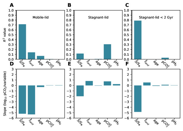
Figure 5: Decomposition of linear correlation coefficients and inferred slope of different prior variables. A-C Correlation coefficients for mobile-lid simulations (A), stagnant-lid simulations (B), and ’young’ ($<2$ Gyr) stagnant-lid simulations (C). D-F Inferred slopes of the different predictor variables for mobile-lid simulations (D), stagnant-lid simulations (E), and ’young’ ($<2$ Gyrs) stagnant-lid planets. Variables not pictured were found to have p-values exceeding the $0.05$ significance threshold in all three cases. Initial pH (pH0) gives $p>0.05$ in the SL (panel B) and young SL (panel C) cases. Note that correlations with pCO2⁰ is performed using $\log_{10}$ pCO2⁰.

In contrast, there is no clear correlation pattern of pCO2 and luminosity in simulations of SL planets (linear correlation coefficient $r^{2}\approx 0.1$, Figure 7B, Figure 5B). However, ’young’ planets (blue dots in Figure 7B) have a stronger linear correlation between $\log_{10}$ pCO2 and $S/S_{\earth}$ ($r^{2}=0.79$ among planets younger than 2 Gyr; Figure 5C). This correlation is even stronger than for the bulk of ML simulations, in which the variance driven by variation in the emerged land fraction $f_{land}$ interplays with luminosity. In addition, the inferred slope of this correlation is very close ($-4.90\pm 0.03$ $\log_{10}$(bar) $(S/S_{\earth})^{-1}$; Figure 5F) to the luminosity-CO2 correlation slope estimated for ML simulations ($-5.02\pm 0.03$ $\log_{10}$(bar) $(S/S_{\earth})^{-1}$; Figure 5D).

In sum, despite not having continental weathering as a negative feedback to atmospheric CO2, SL planets may exhibit the same correlation between pCO2 and luminosity as ML planets. This correlation is lost with planet age, which in our model is a direct proxy for volcanic outgassing (Figure 1C). Through Equation (24), the seafloor weathering feedback to atmospheric CO2 depends on the rate of volcanic outgassing, as fresh basalt need to be resupplied for weathering to occur continuously. Hence, SL planets may lack long-term control of atmospheric CO2, not because they lack continental weathering, but because their volcanic output may halt earlier than that of ML planets.

In our simulations, older SL planets (age $>2$ Gyr) show a more complex distribution of pCO2. At low luminosity ($S/S_{\earth}<0.6$), the distribution is close to uniform between pCO2$\approx 10^{-4}$ bar and pCO2$\approx 0.5$ bar (Figure 7B). At $S/S_{\earth}\approx 0.6$, the distribution becomes bimodal (Figure 7C), with simulations clustering around pCO2$\approx 10^{-4}$ bar, and around pCO2$\in[10^{-1},10^{-0}]$ bar. The simulations of these older SL planets are characterized by low or non existent weathering and volcanic dynamics (Figure 1C). As a result, their atmospheric CO2 dynamics should be dominated by photochemistry. The analysis of the balance between photochemical sources and sinks in those simulations supports that. Indeed, in calculations in which pCH4 and pH2 are constrained to their simulation-average final value, net CO2 photochemical production is predicted when p$\ch{CO2}\lessapprox 10^{-4}$ bar and net removal when p$\ch{CO2}\gtrapprox 10^{-4}$ bar (Figure 2A). Hence, under this approximation on pCH4 and pH2, p$\ch{CO2}\approx 10^{-4}$ bar is predicted to be the steady state value of atmospheric CO2 based solely on photochemical fluxes. Under the alternate approximation of pCH4 and pH2 being fixed at their average final value in simulations that have final pCO2$>10^{-3}$ bar, photochemical calculations no longer predict the existence of a steady-state for pCO2 for $S/S_{\earth}>1.0$ (Figure 2B). In consequence, we propose two explanations for the relatively high final pCO2 simulations observed at $S/S_{\earth}>1.0$ (Figure 7B). They may result from CO2 photochemical accumulation being slow (as photochemical fluxes of CO2 are typically low, Figure 2A). Thus, at our maximum simulation time of 50 Myr, these simulations would still be away from equilibrium, but without having exceeded the pCO2$=1$ bar maximum that we impose. Alternatively, more complex interactions between atmospheric CH4, H2 and CO2 could lead to steady-states observed in our simulations (Figure 7B) but not predicted by our previous approximations (Figure 2).

Figure 6: Steady-state atmospheric concentration of CO2 as a function of the initial value of pCO2. Grey circles are mobile-lid interior convection regime simulations (ML), serving as the uncorrelated control for the stagnant-lid interior convection regime simulations (SL) with age greater than 2 Gyrs (orange circles).

Thus, in the case of older ($>2$ Gyr) SL simulations, the atmospheric state of SL planets exhibits bistability, with the initial p$\ch{CO2}$ becoming an important determinant of the equilibrium p$\ch{CO2}$ (Figure 5B). For instance, an individual volcanic event occurring 2 billion years or more after planetary formation could result in an abrupt change in steady-state p$\ch{CO2}$ (Figure 6). Hence, there might be fundamental unpredictability of the atmospheric concentration of CO2 for SL planets that have exhausted their internal heat budget.

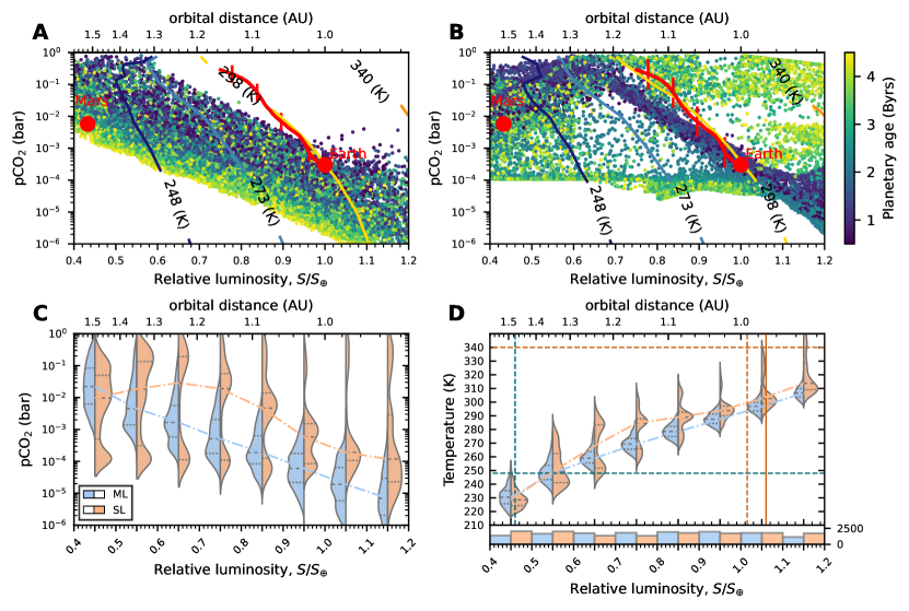
Figure 7: Effect of relative luminosity, $S/S_{\earth}$, on simulated steady-state atmospheres ($p\ch{CO2}$, temperature). A Terrestrial exoplanets in the mobile-lid (ML) interior convection regime. B Terrestrial exoplanets in the stagnant-lid (SL) regime. C,D Distributions of simulations across a discretized range of $S/S_{\earth}$. In A,B, simulation points are colored according to the planetary age used as a model parameter (planets with an age similar to Earth appear in yellow). Red circles indicate modern Earth and Mars. Nominal Earth’s trajectory (change in luminosity and pCO2 over time; Krissansen-Totton et al., 2018) is represented with the red line ending with modern values (red circle), intersecting vertical lines are placed at 1, 2, and 3 Byrs from formation. The dark blue, light blue, gold, and orange contour lines indicate temperatures of 248 K, 273 K, 298 K, and 340 K respectively, predicted from the climate model ran with fixed average values for $p\ch{CH4}$ and $p\ch{H2}$. Linear regression of $p\ch{CO2}$ versus $S/S_{\earth}$ infers a slope (in units of $\log_{10}$(bar) $S_{\earth}^{-1}$) of $-5.02\pm 0.03$ (standard deviation) with correlation coefficient value $r^{2}=0.72$ in A, and $-2.02\pm 0.05$ with correlation coefficient value $r^{2}=0.12$ in B. In C,D, blue (left part of each distribution graph) and orange (right) distributions are compiled from simulations in the ML and SL regimes, respectively. Dot-dashed lines indicate median values. The relative height of the distributions scales with the number of (successful) simulations in each bin. In C, only 1-bar atmospheres are simulated hence no simulation can exceed 1 bar CO2. In D, the horizontal blue dashed line (lower straight line) corresponds to the temperature of 248 K, at which Charnay et al. (2013) report global glaciation including at the equatorial band. The vertical blue dashed line (to the left) corresponds to the OHZ of 1-bar atmosphere planets reported by Kopparapu et al. (2013). The horizontal orange dashed line (upper) corresponds to the 340 K temperature, at which Kopparapu et al. (2013) calculate that depletion of the water reservoir through hydrogen escape can occur on the timescale of Earth’s age. The vertical orange dashed line (to the right) corresponds to the moist runaway inner Habitable Zone limit, and the solid orange line corresponds to the greenhouse runaway limit (Kopparapu et al., 2013). The inset below shows the number of (successful) simulations per bin in either SL or ML regime.

3.2 Influence of interior convection regime on climate and habitability.

Most (about 80%) simulations in both SL and ML interior convection regimes have temperatures comprised between 248 K (global glaciation; Charnay et al., 2013) and 340 K (water runaway; Kopparapu et al., 2013). ML simulations (with continental weathering) are slightly more likely to have a temperate climate (84%) than their SL counterparts without continental weathering (76%), with the caveat that global temperature may be overestimated in some of the SL simulations (cluster of simulations at $10^{-4}$ bar CO2, discussed above). Glacial climates ($T_{surf}<248$ K) were slightly less frequent in the ML regime (16%) than in the SL regime (23%). Per the same caveat discussed above, the actual proportion of glacial climates for SL planets could be greater. Runaway hot climates ($T_{surf}>340$ K) were virtually equal in SL simulations (2%) and in ML simulations (0%).

In spite of fundamental unpredictability of pCO2 on SL planets, their climate turns out to be rather narrowly constrained, and similar to ML planets (Figure 7D). This challenges the view that SL planets would in general have unstable climates and experience either snowball or greenhouse runaway. Instead, terrestrial planets in the SL regime could still be frequently observed in a temperate climate stage of their geological history ($T_{surf}\in[248,340]$ K), despite a relatively short-lived volcanic output. This can be explained by photochemistry providing a stabilizing effect on pCO2, (Figure 2B). Although photochemistry has a weak effect on pCO2, with little dependence on luminosity, the stabilization outcome observed at low volcanic outgassing (or equivalently with age $>2$ Gyrs) may result –by chance– in a temperate climate.

Noticingly, at low values of relative luminosity ($S/S_{\earth}<0.7$), a subset of simulations in the SL regime lead to more clement temperature ($\approx 280$ K) than their ML counterparts (Figure 7D). SL simulations often have higher equilibrium pCO2 than ML simulations at these luminosities (Figure 7C). It may be that both young and old SL planets have relatively high equilibrium pCO2, whereas only young ML planets can have such high equilibrium pCO2 at $S/S_{\earth}<0.7$ (Figure 7A,B). Therefore, SL planets may be more likely to sustain liquid water on their surface at low luminosity/large orbital radius than ML planets would.

3.3 Predictions at planet population scale and prospects for future testing of hypotheses

Our results show that terrestrial planets in the SL regime may not be statistically less frequently habitable than planets in the ML regime. Yet, this may largely be unrelated to the odds of inhabitation of planets in the ML vs. SL regimes, which depends on unknown or poorly constrained factors. These odds could actually differ markedly. It may be that when in the SL regime, terrestrial planets have a climate more sensitive to perturbations, as hinted by the bimodal distribution shown in Figure 7B (and Figure 2B). Thus, advancing the search for biological activity on terrestrial exoplanets would still benefit from observations designed to test whether a sample of terrestrial planets in the HZ of their host star are in the ML or SL regime.

To assess the performance of different observation strategies in inferring the most plausible dominant interior convection regime in terrestrial exoplanets, we calculate the risk of insufficient Bayesian evidence in favor of whichever hypothesis we assume is correct. Hypotheses to be tested using a sample of exoplanet atmosphere data are defined as:

Hypothesis 1

$\mathrm{H}_{ML}$: All terrestrial planets in the HZ have both continental weathering and seafloor weathering (ML regime).

Hypothesis 2

$\mathrm{H}_{SL}$: All terrestrial planets in the HZ only have seafloor weathering (SL regime).

To prospectively test these hypotheses, we focus on $p\ch{CO2}$ as an observable, and the incident flux $S/S_{\earth}$ as a ’contextual’ observable (Catling et al., 2018a).

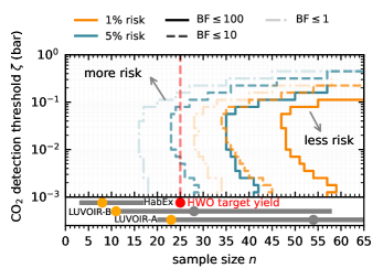
Figure 8: Inference risk (Equation 34) over strategies of CO2 detection threshold ($\zeta$) and sample size ($n$). Orange (blue) lines indicate 1% (5%) risk contour levels. Continuous lines map the risk that evidence in favor of the correct hypothesis is less than ”extreme” (BF$<$100). Dashed lines are contours of the risk that evidence in favor of the correct hypothesis is less than ”strong” (BF$<$10). Semi transparent dashed and dotted lines are contours of the risk that a sample yields stronger evidence in favor of the incorrect hypothesis than in favor of the correct one. The inset at the bottom shows the expected yield of different concepts of space observatories: Large UV/Optical/IR Surveyor (LUVOIR, The LUVOIR Team, 2019), Habitable Exoplanet Observatory (HabEx, Gaudi et al., 2020), and Habitable Worlds Observatory (HWO, Mamajek & Stapelfeldt, 2023). The gray lines and circles indicate the expected number of exo-Earth candidates (EECs) detected by each mission. Orange dots indicate the expected number of EECs spectra from each mission. The red dot indicates the target EEC spectra yield from the most recently proposed mission concept HWO.

To measure the performance of an observation strategy (defined below), we calculate the probability or risk that a sample $X$ resulting from this strategy yields Bayesian evidence in favor of the correct hypothesis $\text{BF}_{\mathrm{H}_{true},\mathrm{H}_{false}}$ smaller than $\eta$ :

$$\begin{split}\rho=max[&P(\text{BF}_{\mathrm{H}_{ML},\mathrm{H}_{SL}}(X^{\mathrm{H}_{ML}})<\eta),\\ &P(\text{BF}_{\mathrm{H}_{SL},\mathrm{H}_{ML}}(X^{\mathrm{H}_{SL}})<\eta)].\end{split}$$ (34)

Bayesian evidence is calculated using the Bayes factor BF (see e.g. Kass & Raftery, 1995)

$$\text{BF}_{\mathrm{H}_{a},\mathrm{H}_{b}}=\frac{P(X|\mathrm{H}_{a})}{P(X|\mathrm{H}_{b})}.$$ (35)

Equation (35) quantifies how much more likely the sample $X$ is under $\mathrm{H}_{a}$ than under $\mathrm{H}_{b}$. While $\text{BF}_{\mathrm{H}_{a},\mathrm{H}_{b}}>1$ technically constitutes evidence in favor of $\mathrm{H}_{a}$, it is common to classify Bayesian evidence according to Jeffrey’s scale: anecdotal ($\text{BF}_{\mathrm{H}_{a},\mathrm{H}_{b}}\in[1,3[$), substantial ($[3,10[$), strong ($[10,100[$), and very strong or decisive ($\geq 100$; Kass & Raftery, 1995; Jeffreys, 1967).

In Equation (34), the Bayes factor is calculated in the case where $\mathrm{H}_{SL}$ is true and $\mathrm{H}_{ML}$ is the null hypothesis, as well as in the case where $\mathrm{H}_{ML}$ is true and $\mathrm{H}_{SL}$ is the null hypothesis. We define an observation strategy as the combination of the number of observed targets (’sample size’, $n$), and the minimal abundance of atmospheric CO2 that can be detected by the hypothetical instrument (’CO2 detection threshold’, $\zeta$). The resulting sample is a series of pairs $X_{n,\zeta}=\{(S/S_{\earth})_{i},\Gamma_{i}\}_{i\in[1,n]}$, where $\Gamma_{i}=1$ if $p\ch{CO2}|_{i}>\zeta$ and 0 otherwise. The likelihood of such a sample under hypothesis $\mathrm{H}$ is then expressed as

$$\begin{array}[]{rcl}P(X_{n}|\mathrm{H})&=&P(\{\Gamma_{i},(S/S_{\earth})_{i}\}_{i\in[1,n]}|\mathrm{H})\\ &=&\prod_{i\in[1,n]}P((\Gamma_{i},(S/S_{\earth})_{i})|\mathrm{H}).\end{array}$$ (36)

We approximate the values of $P((\Gamma_{i},(S/S_{\earth})_{i})|\mathrm{H})$ using our simulations by discretizing $S/S_{\earth}$ and assessing the frequency of $\Gamma$ in the resulting intervals

$$P((\Gamma_{i},(S/S_{\earth})_{i})|\mathrm{H})\approx\frac{\sum_{j\in\mathbf{k}_{\mathrm{H}}}\Gamma(p\ch{CO2}|_{j})}{\sum_{j\in\mathbf{k}_{\mathrm{H}}}{j}}$$ (37)

where the vector $\mathbf{k}_{\mathrm{H}}$ contains the indices $j$ of all simulations of hypothesis $\mathrm{H}$ that verify $(S/S_{\earth})_{j}\in[(S/S_{\earth})_{i}-0.05,(S/S_{\earth})_{i}+0.05[$.

The number of possible combinations of $\{\Gamma_{i},(S/S_{\earth})_{i}\}_{i\in[1,n]}$ increases rapidly with the sample size $n$ (for instance, positive CO2 detection in 15 candidates out of 30 corresponds to $10^{20}$ sets of pairs of $(\Gamma,S/S_{\earth})$). Thus, approximating $P(\text{BF}(X)>\eta)$ requires to resample a large number of samples $X$ from the simulated populations of SL and PT. We find that resampling 200,000 times is largely sufficient to estimate $P(\text{BF}(X)>\eta)$ from the frequency of $\text{BF}(X)>\eta$, even at relatively large sample size (Figure 9).

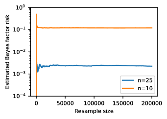
Figure 9: Estimate of the Bayes factor risk (Equation 34) as a function of the resample size (number of generated samples). A CO2 detection threshold $\zeta=10^{-2}$ was used.

The probability that a survey results in unsatisfying evidence decreases both with sample size $n$ and with CO2 detection threshold $\zeta$ as long as $\zeta\gtrapprox 10^{-2}$ bar (Figure 8). However, for relatively high values of $\zeta$ ($\zeta\approx 10^{-1}$ bar; lower characterization effort), increasing sample size has a limited, if not negligible payoff in terms of expected evidence yield. Similarly, at relatively small sample sizes (10 to 25), the value of $\zeta$ has a low incidence on the evidence yield ($\zeta\in[10^{-3},10^{-1}]$ bar). In addition, decreasing the value of $\zeta$ below $\approx 10^{-2}$ is counterproductive as it increases the risk of unsatisfying evidence (for constant $n$; Figure 8). This is due to the fact that in our hypothetical samples, characterization of atmospheric CO2 is assigned a boolean variable according to whether the actual CO2 partial pressure is greater than $\zeta$ or not. Hence, there must be a lower boundary to $\zeta$ such that no information is contained in the sample as all our simulations would have p$\ch{CO2}>\zeta$. Conversely, there must also exist an upper limit to $\zeta$ that leads to a survey yielding no information at all. In between those limits, there is a value of $\zeta$ for which maximum separation between SL and ML simulations is achieved.

The map of the inference risk (Figure 8) suggests that such an optimal value is situated between $10^{-2}$ and $10^{-1}$ bars. For values of $\zeta$ in this interval, lower than 1% risk of achieving less than very strong evidence ($\text{BF}<100$) is achieved for a sample size comprised between 45 and 50 (Figure 8). Strong evidence (BF$>10$) can be achieved in $\geq 99\%$ of samples with a sample size of 34 or more and a CO2 detection threshold of $2\times 10^{-2}$ bar (see dashed orange line in Figure 8). The same strategy would achieve very strong evidence (BF$>100$) in 95% of samples (solid blue line in Figure 8). Hence, such a strategy ($n>34$ and $\zeta\approx 3\times 10^{-2}$ bar) could be optimal if 5% risk of achieving less than decisive evidence and 1% risk of achieving less than strong evidence is acceptable.

The target yield for exo-Earths candidate planetary spectra of LUVOIR (11–23, The LUVOIR Team, 2019) and HabEx (8, Gaudi et al., 2020) could lead to relatively high risk of incorrect inference (Figure 8, inset, orange dots). The target planetary spectra yield for the Habitable Worlds Observatory (25, Mamajek & Stapelfeldt, 2023) is projected to yield strong evidence in $>95$% of samples, but decisive evidence in only $\approx 83$% of samples. However, these probabilities are conditional on the instrument being able to produce acceptable signal to noise ratio for a CO2 spectral feature corresponding to $\approx 2\times 10^{-2}$ bar of CO2 in the atmosphere of all characterized candidates.

4 Discussion

In our simulations, the interior convection regime (stagnant or mobile lid) only had a minor influence on the expected frequency of terrestrial planets with a temperate climate among those that are in the Habitable Zone (HZ) of their host star; the frequency is only slightly lower if stagnant-lid (SL), rather than mobile-lid (ML), is the typical interior convection regime. A strength of our study is the large number of planets for which we have been able to simulate their climate evolution, accounting for different geochemical mechanisms that we have coupled together. As a trade-off of building such a coupled and general model, we have had to make simplifying assumptions, and discard simulations that encountered numerical issues. Together, these lead to several caveats in how our result can be used to tackle future observations of the atmospheres of terrestrial exoplanets. We used a 1-D climate model, and interpolated between pre-simulated grid points which only gives a rough approximation of the surface temperature (Figure 4). We also initialized these climate simulations with a vertical water profile that is not the one typically used in calculations of the inner edge of the HZ (greenhouse runaway). All of our simulations assume that surface liquid water is present, and simulations that dynamically exit the phase space in which the climate model can reach radiative equilibrium were terminated and discarded (Appendix C).

Despite that, we did find simulations that have final states inconsistent with the habitable zone assumptions. Some simulations rest at surface temperature exceeding the estimated onset of greenhouse runaway (340 K; Kopparapu et al., 2013) or below the threshold for global freezing (248 K Charnay et al., 2013). As described in the Results section, the frequency of these occurrences is similar ($\pm 10\%$) between scenarios. In Appendix C, we show that ML simulations are less than $10\%$ more likely to converge than SL ones. Among the causes to simulations being terminated and discarded, only some may count towards “uninhabitable” surface conditions (e.g. encountering states in which the climate model does not converge to radiative equilibrium) while others are purely numerical (stiff integration points).

Hence, our work cannot conclusively quantify the frequency of habitable surface conditions that one may expect in terrestrial planets in the HZ. Instead, our simulations suggest that in a sample of terrestrial planets in the HZ, whichever interior convection regime is most common should not play a critical role in determining the fraction of these planets that have surface conditions permitting liquid water at a given observation time. However, our simulations align with expectations that interior convection regime may be critical in determining whether a terrestrial planet can sustain surface liquid water over more than $\approx 2$ Gyrs. As a consequence, it is useful to design observational strategies that may enable a future telescope to infer which end-member interior convection regime terrestrial planets orbiting other FGK stars lean more towards.

In samples drawn from our simulations, inference of the interior convection regime that dominates in terrestrial exoplanets in the HZ is achieved with “decisive evidence” ($\mathrm{BF}\geq 100$) in $\geq 99\%$ of samples of 45 exoplanets for which detection of CO2 is guaranteed if at a partial pressure of $0.01$ bar or above. Inference in a sample size of 25 yields strong true positive evidence ($\geq 10$) in $\geq 95\%$ of samples.

Bayes factor approaches, such as the one we use, quantify the information gain of sampling, making our analysis agnostic to prior beliefs on which convection regime is most frequent (Jeffreys, 1967). Our simulations assume a random initial state and are solved for the 10 to 100 Myrs equilibrium timescale of atmospheric evolution. Thus the results are robust to uncertainties regarding stochastic events that could influence the global climate such as impacts or individual volcanic events, as such events can be assumed time-independent on a billion-year timescale.

Crafting a null hypothesis is crucial to interpret empirical observations. It is not obvious what should be the null hypothesis whose rejection would mean that terrestrial planets have continental and seafloor weathering as a mechanism that ensures temperate climates across the range of luminosity that spans the HZ. Examples in the solar system (Solomatov & Moresi, 1996), as well as recent planetary interior modeling (Dorn et al., 2018; Foley & Smye, 2018) allowed us to flesh out a credible alternate hypothesis. Namely, we leveraged the possibility that terrestrial planets may have a weaker mode of silicate-carbonate weathering, as a plausible alternative to the hypothesis that planetary habitability within the HZ is supported by Earth-like weathering of sub-aerial continental crust in addition to seafloor dissolution.

Detection threshold	Risk level	Sample size
$\zeta$	$\rho$	$n$
$10^{-3}$ bar	1%	34
$10^{-2}$ bar	1%	25
$10^{-1}$ bar	1%	36
$10^{-3}$ bar	5%	24
$10^{-2}$ bar	5%	18
$10^{-1}$ bar	5%	26

Table 1: Required sample size for selected combinations of $\ch{CO2}$ detection thresholds and accepted risk of Bayes factor evidence being less than 100. See text and Methods for computational details.

Despite geophysical control over atmospheric CO2 existing in both interior convection regimes, the surface temperature is found to increase with luminosity. Thus, the direct effect of increasing luminosity on surface temperature overcompensates the indirect effect of decreasing the equilibrium pCO2. Barring episodes of snowball or hothouse Earth, others who used a model slightly simpler than the one presented here, have suggested that on the billion-year timescale, there has been no or very little trend in the Earth’s global surface temperature (Krissansen-Totton et al., 2018). Our simulations appear to contradict this modeling outcome (Figure 7A,B). It is generally assumed that Earth’s climate was stabilized by the carbonate-silicate geological carbon cycle (as well as seafloor weathering) reducing the concentration of CO2 in the atmosphere as the luminosity of the Sun increased. By relaxing the relation between age and luminosity assumed for calculations of Earth’s climate evolution it appears that seafloor weathering neither alone nor in combination with continental weathering is a sufficient control of atmospheric carbon to entirely compensate the effect of luminosity. As a consequence, it is possible that the Earth’s relatively stable temperate climate over geological times is not due entirely to the stabilizing effect of the carbonate/silicate weathering cycle, but also to the concurrent changes of the Sun’s luminosity (increasing) and the Earth’s outgassing rate (decreasing).

Tosi et al. (2017) and Foley & Smye (2018) have suggested that the stabilization of the climate of SL planets may be limited by the supply of fresh rock associated with volcanic outgassing. In agreement with these expectations, using the outgassing parameterization proposed by Krissansen-Totton & Catling (2017), together with the age-outgassing parameterization of Dorn et al. (2018) results in simulations of SL regime planets that show almost no weathering climate feedback after $\approx 2$ Byrs. This further confirms that planetary age plays a critical role in the habitability of SL planets (Foley & Smye, 2018).

Importantly, we used only a single nominal parameterization for the evolution of volcanic outgassing ($F_{out}$), and single values for each parameter of the weathering functions (see Appendix Table 3). The availability of alternate models for the evolution of volcanic outgassing on SL worlds is limited (an alternative to the parameterization that we used can be found in Foley & Smye, 2018), and their uncertainty is poorly evaluated. Further research of the geological past of Mars and Venus is required to ground models of the evolution of the outgassing rate of stagnant lid worlds and constrain its variability. Krissansen-Totton et al. (2018) proposes ranges of values for the parameters of Earth’s volcanic outgassing over time, as well as for the parameters of seafloor and continental weathering. Future studies will be needed to evaluate the sensitivity of our climate predictions for SL and ML worlds to the values of these parameters. However, this will likely be challenging as many of these parameters have correlated effects on the model. For example, in the model from Krissansen-Totton et al. (2018) that we use, weathering rates are functions of the outgassing rate and other parameters (such as their modern value, see e.g. Equation 24). Hence, changing the value of these parameters is of equivalent scope to changing the outgassing rate $F_{out}$, which is directly a function of age in our model. Additionally, Lehmer et al. (2020) show that variation of parameters in this model of the carbonate-silicate weathering cycle and climate does not wash out the correlation they predict between pCO2 and host star luminosity. In sum, it is possible that introducing variation in most of these parameters will result in different age-atmospheric composition distributions of outputs, but not in different luminosity-atmospheric composition distributions. Given the large number of processes that interact in our model, we argue that selecting nominal models for outgassing and weathering in SL and ML worlds is an important first step, which is required to disentangle the effect of each process on the steady-state atmospheric composition.

The Earth, Venus, and perhaps Mars, have not been in any one single tectonic regime during the entirety of their geological history, instead they may have undergone shifts between modes, a regime described as ’episodic’ (Moresi & Solomatov, 1998). This scenario is not explicitly modeled here. By running our model from random initial conditions until an equilibrium for a fixed outgassing rate is found, each simulation is agnostic to the planet’s past. However, the planet’s internal heat dissipates at different rates according to their mantle’s convection regime. Hence, if a planet changes convection regime after significant time spent in the alternate one, their outgassing rate at a given age will likely differ significantly from the parameterizations we use here. Therefore, the luminosity-pCO2 distributions that we simulate under the two end-member regimes should not be affected by planets having undergone a different tectonic mode in their past, but the age-pCO2 distributions might.

Our simulations are seeded with random initial conditions, thus assessing the possibility for multiple equilibria to exist for a given pair of values for outgassing and luminosity. Doing so reveals that the absence of continental weathering and outgassing on SL planets older than 2 Byrs may cause bistability of their climate. An event releasing large amounts of CO2 to the atmosphere, without equivalent supply of fresh rock, would then result in an inescapably CO2-rich atmosphere, regardless of luminosity. However, our model also suggests that such random events may not be required for CO2 runaway atmospheres under relatively high incident luminosity, as photochemistry can then lead to slow CO2 accumulation (Figure 2B).

Our model revealed that weak or absent outgassing, limited or absent supply of weatherable rock (as one might expect on a relatively old world subject to stagnant-lid mantle convection), leads to atmospheric CO2 dynamics being dominated by photochemistry, resulting in equilibrium pCO2 (high or low) dependent on simulation initial conditions when luminosity is between 0.7 and 1 $S_{\earth}$. Hence, if certain trajectories of atmospheric evolution on the billion years scale favor one scenario over the other (CO2-rich or CO2-poor), then warm climates on SL worlds may be more frequent than we predict (if CO2-rich is more likely), or the overlap in the luminosity-CO2 distribution between SL and ML worlds may be greater than we estimate (if CO2-poor is more likely). Albeit beyond the scope of this study, the coupled model presented here could be used to run long-term (several billion years) simulations, and include random perturbations in order to better constrain the long-term climate dynamics.

The sample size targeted by the Habitable Worlds Observatory (HWO) is 25 Earth-mass planets in the HZ of FGK stars (Mamajek & Stapelfeldt, 2023). Lehmer et al. (2020) calculated that such sample size would be insufficient to reject log-uniform distribution of CO2 with respect to luminosity. By using a likelihood ratio approach and an explicit alternate hypothesis, we find that a sample size of 25 is likely ($\approx 83$%) to provide decisive evidence ($>100$), and extremely likely ($\approx 96$%) to provide strong evidence ($>10$) for the inference of the dominant interior regime. According to our model, this evidence yield can be achieved for a sample size of 25 exoplanets if the characterization effort for each of them guarantees that CO2 above $0.01$ bar would lead to positive detection in the spectrum. However, the proposed target sample for the HWO includes different star types while our model assumes a Sun-like (type G) star. If variation in star spectra across the HWO target sample was to significantly alter the distribution of atmospheric CO2, then the required sample size could differ from our estimate. In addition, whether a sample size of 25 roughly Earth-mass planets orbiting FGK stars is attainable within the constrains posed on future instruments is uncertain. Earth-like planets around FGK stars have not been yet detected, possibly due to instrument limitations, leading yield estimates of missions to rely on occurrence rates of such planets (noted $\eta_{\bigoplus}$) obtained from models. The PLATO mission (Rauer et al., 2024), scheduled to launch in 2026 is designed to fill this gap, and permit the detection and characterization of bulk properties of Earth-sized planets orbiting FGK stars.

The distribution of the radius of planets in the target sample of the HWO varies around one Earth radius. Planetary radius (more precisely planetary mass) is a key parameter determining the heat budget and thus affects not only the volcanic outgassing rate but also the likelihood of different interior convection regimes (Dorn et al., 2018). As a consequence, the population from which the Habitable Worlds Observatory would sample could differ from the one we simulate. In particular, by adding variability in planetary radius, it is likely that the spread of the expected $S$-pCO2 relation be increased, thus increasing the overlap between the two scenarios of interior convection regimes and subsequently increasing the required sample size.

The required sample size might, however, be reduced, in three ways. The prospective analysis presented here assumes that the sample is composed of independent observations, however, one may increase efficiency by adopting a sequential strategy such that each new observation is targeted in such a way that its addition to a known sample maximizes information gain. With moderate effort, one could refine the fixed Bayes Factor design we have studied into a so-called Sequential Bayes Factor design and analyze its effectiveness (Schönbrodt & Wagenmakers, 2017). Bixel & Apai (2020) have suggested using inferred planetary age to increase the statistical power of life detection surveys. Apart from the interior convection regime, atmospheric abundance of CO2 may hence be chiefly determined by luminosity/orbital radius, planetary age, and planetary mass. All of these quantities could be estimated when characterizing an exoplanet. Planetary mass and age could eventually be included in a more sophisticated prospective statistical test in order to quantify the gain of retrieving such parameters on the required sample size. Future work may also aim at relaxing the assumption of 1 Earth-mass planets by linking volcanic outgassing to planetary mass (e.g. following Dorn et al., 2018), as well as the assumption of a strictly Sun-like star by running additional simulations of the atmospheric model Atmos.

Ultimately, the feasibility of the 0.01 bar limit of detection of CO2 depends on exoplanet survey mission design on the one hand, and on the distance of the sampled exoplanets to us and to their star in the case of a direct imaging survey such as the Habitable Worlds Observatory, or on the orbital period for transit-based proposed architectures (e.g. the Nautilus concept; Apai et al., 2019). Whether such limit of detection can be achieved for 25 candidates will be critically important for the design of any future exoplanet observatory. In future work, coupling our simulations with planetary spectra generators (Villanueva et al., 2018) and survey simulators that integrate exoplanet catalog to simulate realistic exoplanet samples (Bixel & Apai, 2021) will help link instrument design parameters with our CO2 limit of detection parameter. Doing so will enable to more directly identify the optimal compromise between instrument cost and scientific gain.

Appendix A Model parameters

parameter	meaning	distribution	range	unit
$p\ch{H2}^{0}$	initial $p\ch{H2}$	Log-Uniform	$10^{-5}-10^{-2}$	bar
$p\ch{CO2}^{0}$	initial $p\ch{CO2}$	Log-Uniform	$10^{-4}-0.5$	bar
$p\ch{CH4}^{0}$	initial $p\ch{CH4}$	Log-Uniform	$10^{-6}-10^{-4}$	bar
$p\ch{CO}^{0}$	initial $p\ch{CO}$	Log-Uniform	$10^{-6}-10^{-4}$	bar
pH^0	initial pH	Uniform	6.5-7.5
$f_{land}$	emerged land surface fraction	Uniform	0.0-0.35
$\tau$	planet age	uniform	0.5-4.5	Gyr
$S/S_{\oplus}$	Relative luminosity	uniform	0.4-1.2	$S_{\oplus}$

Table 2: Planetary parameters and initial values of time-dependent variables and their distributions

Table 3: Physical and chemical constants.

Parameter	Value	Unit	Description	Reference
$v_{\ch{H2}}$	$1.3\times 10^{-2}$	$\text{cm}~{}\text{s}^{-1}$	SBL piston velocity of $\ch{H2}$	Sauterey+ 2020
$v_{\ch{CO2}}$	$4.8\times 10^{-3}$	$\text{cm}~{}\text{s}^{-1}$	SBL piston velocity of $\ch{CO2}$	Sauterey+ 2020
$v_{\ch{CH4}}$	$4.5\times 10^{-3}$	$\text{cm}~{}\text{s}^{-1}$	SBL piston velocity of $\ch{CH4}$	Sauterey+ 2020
$v_{\ch{CO}}$	$4.8\times 10^{-3}$	$\text{cm}~{}\text{s}^{-1}$	SBL piston velocity of $\ch{CO}$	Sauterey+ 2020
$\alpha_{\ch{H2}}$	$7.8\times 10^{-4}$	$\text{mol}~{}\text{L}^{-1}~{}\text{bar}^{-1}$	Henry coefficient for $\ch{H2}$	Sauterey+ 2020
$\alpha_{\ch{CO2}}$	Supp. Methods B.1	$\text{mol}~{}\text{L}^{-1}~{}\text{bar}^{-1}$	Henry coefficient for $\ch{CO2}$	Sauterey+ 2020
$\alpha_{\ch{CH4}}$	$1.4\times 10^{-3}$	$\text{mol}~{}\text{L}^{-1}~{}\text{bar}^{-1}$	Henry coefficient for $\ch{CH4}$	Sauterey+ 2020
$\alpha_{\ch{CO}}$	$1\times 10^{-3}$	$\text{mol}~{}\text{L}^{-1}~{}\text{bar}^{-1}$	Henry coefficient for $\ch{CO}$	Sauterey+ 2020
$C$	$6.02\times 10^{20}$	$\text{L}~{}\text{mol}^{-1}~{}\text{cm}^{-3}$	Unit conversion constant
$P_{tot}$	1	bar	Total atmospheric pressure	assumed
$S_{p}$	$5.1\times 10^{18}$	cm2	Planetary surface area
$M_{air}$	28.16 $\times 10^{-3}$	$\text{kg}~{}\text{mol}^{-1}$	Air molar mass	Sauterey+ 2020
$n_{tot}$	$P_{tot}S_{p}\times 10^{-5}/(gM_{air})$	mol	Total air mol
$g$	$9.80$	m s-2	Earth’s gravitational acceleration
$pK_{w}$	14		Water ionic constant
$M_{o}$	$3\times 10^{21}$	kg	Ocean mass
$M_{d}$	$0.01\times M_{o}$	kg	Ocean mass
$J$	$J=6.8\times 10^{16}$	kg yr-1	Ocean mixing rate	K-T&C 2017
$k_{hyd}$	$\exp{-\frac{10,570}{T+25.6}}$	$\text{mol}^{-1}~{}\text{s}^{-1}$	$\ch{CO}$ hydratation rate coefficient	Kharecha+ 2005
$k_{2}$	$6.4\times 10^{-5}$	$\text{s}^{-1}$	Rate constant of HCOO- -¿ CO	Kharecha+ 2005
$k_{3}$	$2.7\times 10^{-6}$	$\text{s}^{-1}$	Rate constant of $\ch{HCOO-->CH3COO-}$	Kharecha+ 2005
$\chi$	$0.3$		$\ch{CO2}$ parameter for $F_{carb}$	K-T&C 2017
$\alpha_{s}$	$0.3$		$\ch{CO2}$ parameter for $F_{sil}$	K-T&C 2017
$T_{e}$	$25$	K	weathering e-folding temperature	K-T&C 2017
$T_{ME}$	$15$	∘C	surface temperature of the modern Earth	K-T&C 2017
$f_{land}^{ME}$	$0.29$		modern Earth emerged land fraction	K-T&C 2017
$F_{carb}^{ME}$	$10.5\times 10^{12}$	mol yr-1	carbonate weathering flux on modern Earth	K-T&C 2017
$F_{sil}^{ME}$	$10.5\times 10^{12}$	mol yr-1	silicate weathering flux on modern Earth	K-T&C 2017
$K_{sol}$	Supp. Methods B.2	$\text{mol}^{2}~{}\text{kg}^{-2}$	Solubility product of carbonates	K-T&C 2017
$k_{shelf}$	$1.03\times 10^{13}$	mol yr-1	above shelf reference precipitation rate	K-T&C 2017
$k_{pelagic}$	$1.40\times 10^{12}$	mol yr-1	pelagic reference precipitation rate	K-T&C 2017
$k_{p}$	$5.12\times 10^{11}$	mol yr-1	deep ocean reference precipitation rate	K-T&C 2017
$k_{diss}$	$3.17\times 10^{29}$	mol yr-1	Reference basalt dissolution rate	K-T&C 2017
$pH^{ME}$	8.2		Modern pH of Earth’s ocean
$E_{bas}$	$92$	kJ mol-1	Activation energy of basalt dissolution	K-T&C 2017
$F_{out}^{ME}$	$8.0\times 10^{12}$	mol yr-1	Present day volcanic outgassing of $\ch{CO2}$	K-T&C 2017
$\beta$	$1$		Basalt dissolution sensitivity to basalt supply	K-T&C 2017
$\gamma$	$0.5$		Basalt dissolution sensitivity to pH	K-T&C 2017
$Serp^{ME}$	$10^{11}$	mol yr-1	Modern CH4 production by serpentinization	Sauterey+ 2020
$Volc^{ME}$	$5.35\times 10^{12}$	mol yr-1	Modern volcanic outgassing of $\ch{H2}$	Sauterey+ 2020

Appendix B Chemical equilibria

B.1 Solubility of CO2

From Krissansen-Totton & Catling (2017), we use the following parameterization for the Henry’s law constant of $\ch{CO2}$ solubility as a function of temperature.

$$\begin{split}\alpha_{\ch{CO2}}=10^{-5}\exp\{&(\frac{9345.17}{T}-167.8108+23.3585\log_{e}T\\ &+(0.023517-2.3656\times 10^{-4}T+4.7036\times 10^{-7}T^{2})35.0)\}\end{split}$$ (B1)

$\text{mol}~{}\text{L}^{-1}~{}\text{bar}^{-1}$.

B.2 Solubility product of carbonates in the ocean

The solubility product of the ocean is obtained from Krissansen-Totton & Catling (2017), assuming a salinity of 35 per thousand :

$$\begin{split}\log_{10}K_{sol}=&-171.9065-0.077993T+2839.319/T+71.595\log_{10}(T)\\ &+(-0.77712+0.0028426T+178.34/T)35^{0.5}\\ &-0.0711\times 35.0+0.0041249\times 35^{1.5}\end{split}$$ (B2)

B.3 Carbonate equilibrium constants

The dissociation constants of $\ch{CO2}$ and $\ch{HCO3}^{-}$ are given as functions of temperatures (with a salinity of 35 per thousand:

$$\log_{10}K_{1}(T)=-17.788+0.073104\times T+0.0051087\times 35-1.1463e-4T^{2}$$ (B3)

and

$$\log_{10}K_{2}(T)=-20.919+0.064209\times T+0.011887\times 35-8.7313e-5T^{2}$$ (B4)

Appendix C Non-convergent simulations

In the 20,000 simulations that we have launched for each scenario of interior convection regime, a non-negligible fraction was discarded: ultimately, 14,384 simulations of the stagnant-lid regime, and 15,650 simulations of the mobile-lid regime are retained and used in our analyses. This raises the question that the variability that we introduce in the inputs of our simulations is not entirely carried to the distribution of our outputs. Second, it also raises the question that some equilibrium states of the atmosphere that would be relevant for their implications for habitability are left out of our analyses.

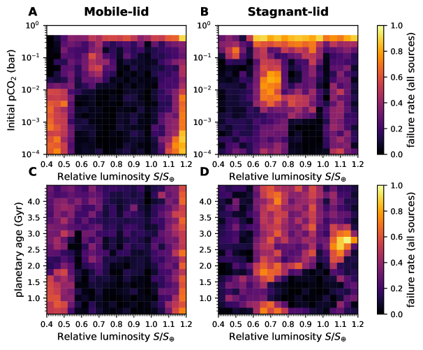
Figure 10: Map of the frequency of simulations that were halted and discarded due to either exceeding the imposed time limit to simulate 50 Myr of atmospheric evolution or reaching inconsistent states in the case of mobile-lid (A,C) or stagnant-lid (B,D) interior convection regime. The row A,B shows this frequency as a function of relative luminosity and initial value of atmospheric CO2, the row C,D shows it as a function of relative luminosity and planetary age.

We identify two modes of failure of simulations. The most frequent one (67% of discarded simulations, 17% of all launched simulations) is that the numerical integration (performed using th backward differentiation formula; Petzold, 1983) gets stuck on so-called ’stiff’ points of the system, corresponding to difficult system states that are unstable. These simulations exceed the allocated compute time as they are terminated after the allocated 4 hours. Then other simulations are halted when they reach states that are outside the boundaries of the atmospheric calculation grid (see Figure 3 for an example of these boundaries). This situation is caught in our model by simply validating whether a step taken by the integrator lies within the convex hull of the grid (Barber et al., 1996; Virtanen et al., 2020). This scenario is identified in 33% of discarded runs (and 8% of all simulations). Overall, factors that most explain simulations failing to reach a consistent final state are the initial value for the CO2 pressure, the value of the relative luminosity, and the value of the planetary age (Figure 10). By launching 20,000 simulations in each interior convection regime, we sample the space of initial parameters well enough that the frequency of runs that successfully reach their end state converges (Figure 11).

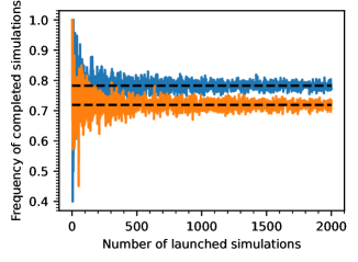
Figure 11: Frequency of runs that are completed before the allocated 4 hours compute time (including runs that are terminated) as a function of the number of launched simulations. The orange line corresponds to simulations in the stagnant-lid regime, the blue line corresponds to simulations in the mobile-lid regime. The dashed black lines highlight the overall average over the 20,000 launched simulations in each regimes. Note that the scale of the x-axis stops at 2,000 launched simulations, out of the total 20,000 launched simulations in order to highlight the convergence to the overall average.

To initialize a simulation, we sample the value for the initial pCO2 independently from the values of age and luminosity as to not introduce any prior assumption on a relation between the final pCO2 and either age or luminosity. Hence, some simulations are initialized in climate and atmospheric regimes that are far from equilibrium as well as unlikely. It is thus expected that a complex model such as ours would experience convergence issues in those cases.

Mobile-lid convection simulations experience most frequent discarding rate at the extremes of the range of values of relative luminosity that we sample from, whereas initial pCO2 and age only have a minor effect on convergence rate (Figure 10A,C). In our model, the grid of atmospheric chemistry and climate calculations is restricted to situations in which radiative equilibrium exists. We run simulations outside of the conditions at which it is commonly assumed that radiative equilibrium exists within temperate climate temperatures (Figure 4B).

Mobile-lid convection regime simulations also fail frequently when initialized with low atmospheric CO2 (p$\ch{CO2}^{0}<10^{-2}$ bar) and low luminosity ($S/S_{\earth}<0.55$; Figure 10A). This is expected because at low luminosity, the equilibrium pCO2 should be relatively high. Thus, simulations initialized far from the equilibrium should more frequently fail to converge.

Stagnant-lid convection regime simulations are halted relatively evenly over the values of luminosity (Figure 10B,D). Stagnant-lid regime simulations converge most frequently when they are initialized with non-negligible volcanic outgassing (age comprised between 1–2 Gyrs). The higher the value of volcanic outgassing ($\approx 1.5$ Gyrs; Figure 1C), the wider the range of luminosities at which a 100% convergence rate is observed (Figure 10D).

Appendix D Multiple linear regression for atmospheric CO2

We performed linear regression between $\log_{10}$ pCO2 and the input variables that cause variability in our system (luminosity, $S/S_{\earth}$, emerged land fraction $f_{land}$, age, initial composition of the simulated atmosphere, initial pH See Figure 5).

In our set of ”mobile-lid” interior convection regime simulations, luminosity is the most variance explaining log-linear factor ($r^{2}=0.72$), then, emerged land fraction and planetary age (proxy to outgassing rate) explain most of the remaining variance ($r^{2}=0.14$ and $r^{2}=0.07$ respectively; Figure 5A). Not all the variance in the synthetic sample is explained by the variance-introducing variables (the multilinear $r^{2}$-value is found to be about 0.97 for the mobile-lid convection regime simulations). This is due to some variance being introduced by discarded simulations, and to the relation between the variables and pCO2 not being exactly log-linear.

Relative luminosity being the most determining factor of atmospheric CO2 highlights that the carbonate-silicate cycle is at the core of the possibility for temperate conditions to exist throughout the habitable zone. However, the importance of age and emerged land fraction seems to often be omitted in astronomical definitions of the HZ (despite being actively discussed in the field of geophysics Lenardic et al., 2016). This importance comes naturally from the fact that the geological carbon cycle model that we use (taken from Krissansen-Totton & Catling, 2017) is dependent on planetary age through the value of volcanic outgassing used in equations 15, 16, and 24, and on the value of the emerged land fraction (assumed to be composed of continental material in the case of mobile-lid convection simulations) through equations 15, 16.

In stagnant-lid convection simulations, luminosity is not the variable with the highest correlation coefficient for $\log_{10}$pCO2, instead, pCO2⁰ the initial CO2 pressure scores the highest correlation coefficient (Figure 5B). In SL simulations, emerged land does not contribute to weathering (Methods), hence SL simulations not showing a linear component in the $f_{land}$-pCO2 space (Figure 5). As luminosity negatively correlate with equilibrium pCO2 (Figure 5D-F), pCO2⁰ positively correlates with equilibrium pCO2 for stagnant-lid regime simulations (Figure 5E).

The log-log correlation between pCO2 and pCO2⁰ in the dataset composed of simulations in the stagnant-lid interior convection regime is absent in the subset of these simulations of age below 2 Gyrs (Figure 5C).

Others have suggested that age-based target selection could reduce required sample sizes for e.g. biosignature assessment (Bixel & Apai, 2020). Our simulations further support this claim, as we find that age and the variables related to it is the secondmost correlating factor to atmospheric CO2 for mobile-lid regime simulations, and as the distribution of equilibrium pCO2 for stagnant-lid regime simulations is qualitatively different for ’old’ and ’young’ planets. Hence, including age in a trend inference framework similar to the one we propose in the Main Text could result in fewer required planet in a sample to infer the dominant convection regime. Because ’old’ stagnant-lid regime simulations have a pCO2–$S/S_{\earth}$ distribution qualitatively different from that of mobile-lid regime simulations (whereas ’young’ mobile-lid regime simulations have a similar distribution), an optimal strategy aimed at inferring the most common interior convection regime in Earth-like exoplanets would probably preferentially target ’old’ ($>2$ Gyrs) targets.

References

- Alt & Teagle (1999) Alt, J. C., & Teagle, D. A. 1999, Geochimica et Cosmochimica Acta, 63, 1527, doi: 10.1016/s0016-7037(99)00123-4
- Apai et al. (2019) Apai, D., Milster, T. D., Kim, D. W., et al. 2019, AJ, 158, 83, doi: 10.3847/1538-3881/ab2631
- Apai et al. (2018) Apai, D., Ciesla, F., Mulders, G. D., et al. 2018, arXiv e-prints, arXiv:1803.08682, doi: 10.48550/arXiv.1803.08682
- Arney et al. (2016) Arney, G., Domagal-Goldman, S. D., Meadows, V. S., et al. 2016, Astrobiology, 16, 873, doi: 10.1089/ast.2015.1422
- Barber et al. (1996) Barber, C. B., Dobkin, D. P., & Huhdanpaa, H. 1996, ACM Transactions on Mathematical Software, 22, 469, doi: 10.1145/235815.235821
- Bar‐Nun & Chang (1983) Bar‐Nun, A., & Chang, S. 1983, Journal of Geophysical Research: Oceans, 88, 6662–6672, doi: 10.1029/jc088ic11p06662
- Bean et al. (2017) Bean, J. L., Abbot, D. S., & Kempton, E. M.-R. 2017, The Astrophysical Journal, 841, L24, doi: 10.3847/2041-8213/aa738a
- Bixel & Apai (2020) Bixel, A., & Apai, D. 2020, The Astrophysical Journal, 896, 131, doi: 10.3847/1538-4357/ab8fad
- Bixel & Apai (2021) —. 2021, The Astronomical Journal, 161, 228, doi: 10.3847/1538-3881/abe042
- Catling & Kasting (2017) Catling, D. C., & Kasting, J. F. 2017, Atmospheric Evolution on Inhabited and Lifeless Worlds (Cambridge University Press), doi: 10.1017/9781139020558
- Catling et al. (2018a) Catling, D. C., Krissansen-Totton, J., Kiang, N. Y., et al. 2018a, Astrobiology, 18, 709, doi: 10.1089/ast.2017.1737
- Catling et al. (2018b) —. 2018b, Astrobiology, 18, 709, doi: 10.1089/ast.2017.1737
- Charnay et al. (2013) Charnay, B., Forget, F., Wordsworth, R., et al. 2013, Journal of Geophysical Research: Atmospheres, 118, 10,414, doi: https://doi.org/10.1002/jgrd.50808
- Cockell et al. (2016) Cockell, C., Bush, T., Bryce, C., et al. 2016, Astrobiology, 16, 89, doi: 10.1089/ast.2015.1295
- Dorn et al. (2018) Dorn, C., Noack, L., & Rozel, A. B. 2018, Astronomy & Astrophysics, 614, A18, doi: 10.1051/0004-6361/201731513
- Fauchez et al. (2021) Fauchez, T. J., Turbet, M., Sergeev, D. E., et al. 2021, The Planetary Science Journal, 2, 106, doi: 10.3847/psj/abf4df
- Foley (2019) Foley, B. J. 2019, The Astrophysical Journal, 875, 72, doi: 10.3847/1538-4357/ab0f31
- Foley & Smye (2018) Foley, B. J., & Smye, A. J. 2018, Astrobiology, 18, 873, doi: 10.1089/ast.2017.1695
- Gaudi et al. (2020) Gaudi, B. S., Seager, S., Mennesson, B., et al. 2020, arXiv e-prints, arXiv:2001.06683, doi: 10.48550/arXiv.2001.06683
- Gillis & Coogan (2011) Gillis, K., & Coogan, L. 2011, Earth and Planetary Science Letters, 302, 385, doi: 10.1016/j.epsl.2010.12.030
- Haqq-Misra et al. (2008) Haqq-Misra, J. D., Domagal-Goldman, S. D., Kasting, P. J., & Kasting, J. F. 2008, Astrobiology, 8, 1127, doi: 10.1089/ast.2007.0197
- Hart (1979) Hart, M. H. 1979, Icarus, 37, 351–357, doi: 10.1016/0019-1035(79)90141-6
- Hessler et al. (2004) Hessler, A. M., Lowe, D. R., Jones, R. L., & Bird, D. K. 2004, Nature, 428, 736–738, doi: 10.1038/nature02471
- Huang (1959) Huang, S.-S. 1959, American scientist, 47, 397, doi: http://www.jstor.org/stable/27827376
- Jeffreys (1967) Jeffreys, H. 1967, Theory of probability., 3rd edn. (Oxford: Clarendon Press)
- Kanzaki & Murakami (2015) Kanzaki, Y., & Murakami, T. 2015, Geochimica et Cosmochimica Acta, 159, 190–219, doi: 10.1016/j.gca.2015.03.011
- Kass & Raftery (1995) Kass, R. E., & Raftery, A. E. 1995, Journal of the American Statistical Association, 90, 773, doi: 10.1080/01621459.1995.10476572
- Kasting (1993) Kasting, J. F. 1993, Science, 259, 920–926, doi: 10.1126/science.11536547
- Kasting et al. (1993) Kasting, J. F., Whitmire, D. P., & Reynolds, R. T. 1993, Icarus, 101, 108, doi: 10.1006/icar.1993.1010
- Kharecha et al. (2005) Kharecha, P., Kasting, J., & Siefert, J. 2005, Geobiology, 3, 53, doi: 10.1111/j.1472-4669.2005.00049.x
- Kopparapu et al. (2013) Kopparapu, R. K., Ramirez, R., Kasting, J. F., et al. 2013, The Astrophysical Journal, 765, 131, doi: 10.1088/0004-637x/765/2/131
- Krissansen-Totton et al. (2018) Krissansen-Totton, J., Arney, G. N., & Catling, D. C. 2018, Proceedings of the National Academy of Sciences, 115, 4105, doi: 10.1073/pnas.1721296115
- Krissansen-Totton & Catling (2017) Krissansen-Totton, J., & Catling, D. C. 2017, Nature Communications, 8, doi: 10.1038/ncomms15423
- Krissansen-Totton et al. (2022) Krissansen-Totton, J., Thompson, M., Galloway, M. L., & Fortney, J. J. 2022, Nature Astronomy, 6, 189, doi: 10.1038/s41550-021-01579-7
- Lehmer et al. (2020) Lehmer, O. R., Catling, D. C., & Krissansen-Totton, J. 2020, Nature Communications, 11, doi: 10.1038/s41467-020-19896-2
- Lenardic et al. (2016) Lenardic, A., Jellinek, A. M., Foley, B., O’Neill, C., & Moore, W. B. 2016, Journal of Geophysical Research: Planets, 121, 1831–1864, doi: 10.1002/2016je005089
- Mamajek & Stapelfeldt (2023) Mamajek, E., & Stapelfeldt, K. 2023, Mission Star List for the Habitable Worlds Observatory, NASA Jet Propulsion Laboratory
- Manabe & Wetherald (1967) Manabe, S., & Wetherald, R. T. 1967, Journal of the Atmospheric Sciences, 24, 241, doi: 10.1175/1520-0469(1967)024<0241:teotaw>2.0.co;2
- Mazevet et al. (2023) Mazevet, S., Affholder, A., Sauterey, B., et al. 2023, Comptes Rendus. Physique, doi: 10.5802/crphys.154
- Meadows et al. (2018) Meadows, V. S., Reinhard, C. T., Arney, G. N., et al. 2018, Astrobiology, 18, 630, doi: 10.1089/ast.2017.1727
- Moresi & Solomatov (1998) Moresi, L., & Solomatov, V. 1998, Geophysical Journal International, 133, 669, doi: 10.1046/j.1365-246X.1998.00521.x
- National Academies of Sciences, Engineering, and Medicine (2021) National Academies of Sciences, Engineering, and Medicine. 2021, Pathways to Discovery in Astronomy and Astrophysics for the 2020s (Washington, DC: The National Academies Press), doi: 10.17226/26141
- Petzold (1983) Petzold, L. 1983, SIAM Journal on Scientific and Statistical Computing, 4, 136, doi: 10.1137/0904010
- Rauer et al. (2024) Rauer, H., Aerts, C., Cabrera, J., et al. 2024, arXiv e-prints, arXiv:2406.05447, doi: 10.48550/arXiv.2406.05447
- Robinson (2018) Robinson, T. D. 2018, Characterizing Exoplanet Habitability (Springer International Publishing), 3137–3157, doi: 10.1007/978-3-319-55333-7_67
- Rye et al. (1995) Rye, R., Kuo, P. H., & Holland, H. D. 1995, Nature, 378, 603–605, doi: 10.1038/378603a0
- Sauterey et al. (2020) Sauterey, B., Charnay, B., Affholder, A., Mazevet, S., & Ferrière, R. 2020, Nature Communications, 11, doi: 10.1038/s41467-020-16374-7
- Schönbrodt & Wagenmakers (2017) Schönbrodt, F. D., & Wagenmakers, E.-J. 2017, Psychonomic Bulletin & Review, 25, 128, doi: 10.3758/s13423-017-1230-y
- Sheldon (2006) Sheldon, N. D. 2006, Precambrian Research, 147, 148–155, doi: 10.1016/j.precamres.2006.02.004
- Sleep & Zahnle (2001) Sleep, N. H., & Zahnle, K. 2001, Journal of Geophysical Research: Planets, 106, 1373, doi: https://doi.org/10.1029/2000JE001247
- Solomatov & Moresi (1996) Solomatov, V. S., & Moresi, L.-N. 1996, Journal of Geophysical Research: Planets, 101, 4737, doi: 10.1029/95je03361
- The LUVOIR Team (2019) The LUVOIR Team. 2019, The LUVOIR Mission Concept Study Final Report, arXiv, doi: 10.48550/ARXIV.1912.06219
- Tosi et al. (2017) Tosi, N., Godolt, M., Stracke, B., et al. 2017, Astronomy & Astrophysics, 605, A71, doi: 10.1051/0004-6361/201730728
- Villanueva et al. (2018) Villanueva, G., Smith, M., Protopapa, S., Faggi, S., & Mandell, A. 2018, Journal of Quantitative Spectroscopy and Radiative Transfer, 217, 86, doi: 10.1016/j.jqsrt.2018.05.023
- Virtanen et al. (2020) Virtanen, P., Gommers, R., Oliphant, T. E., et al. 2020, Nature Methods, 17, 261, doi: 10.1038/s41592-019-0686-2
- von Paris et al. (2008) von Paris, P., Rauer, H., Grenfell, J. L., et al. 2008, Planetary and Space Science, 56, 1244, doi: 10.1016/j.pss.2008.04.008
- Walker et al. (1981) Walker, J. C. G., Hays, P. B., & Kasting, J. F. 1981, Journal of Geophysical Research, 86, 9776, doi: 10.1029/jc086ic10p09776
- Windley et al. (2021) Windley, B. F., Kusky, T., & Polat, A. 2021, Precambrian Research, 352, 105980, doi: 10.1016/j.precamres.2020.105980
- Wolf & Toon (2013) Wolf, E., & Toon, O. 2013, Astrobiology, 13, 656, doi: 10.1089/ast.2012.0936
- Zahnle (1986) Zahnle, K. J. 1986, Journal of Geophysical Research, 91, 2819, doi: 10.1029/jd091id02p02819