Populating Galaxies Into Halos Via Machine Learning on the Simba Simulation

Abstract

We present machine learning (ML)-based pipelines designed to populate galaxies into dark matter halos from N-body simulations. These pipelines predict galaxy stellar mass ($M_{*}$), star formation rate (SFR), atomic and molecular gas contents, and metallicities, and can be easily extended to other galaxy properties and simulations. Our approach begins by categorizing galaxies into central and satellite classifications, followed by their ML classification into quenched (Q) and star-forming (SF) galaxies. We then develop regressors specifically for the SF galaxies within both central and satellite subgroups. We train the model on the $(100\mathrm{h^{-1}Mpc})^{3}$ Simba galaxy formation simulation at $z=0$. Our pipeline yields robust predictions for stellar mass and metallicity and offers significant improvements for SFR and gas properties compared to previous works, achieving an unbiased scatter of less than 0.2 dex around true Simba values for the halo-$M_{\rm HI}$ relation of central galaxies. We also show the effectiveness of the ML-based pipelines at $z=1,2$. Interestingly, we find that training on fraction-based properties (e.g. $M_{\rm HI}$/$M_{*}$) and then multiplying by the ML-predicted $M_{*}$ yields improved predictions versus directly training on the property value, for many quantities across redshifts. However, we find that the ML-predicted scatter around the mean is lower than the true scatter, leading to artificially suppressed distribution functions at high values. To alleviate this, we add a “ML scatter bias”, finely tuned to recover the true distribution functions, critical for accurate predictions of integrated quantities such as H i intensity maps.

1 Introduction

The connection between galaxies and their host dark matter halo has long been one of the most important areas of research in cosmology and galaxy evolution. Halos are essentially the building blocks of large-scale structures, where baryonic matter condenses to form individual galaxies, groups, and clusters. Large cosmological N-body simulations can self-consistently model the evolution of halos and give us a detailed insight into their abundance, clustering, and substructure in a $\Lambda$CDM universe.

In contrast to halos, simulations have greater challenges with modeling the baryonic content of galaxies (Somerville & Davé, 2015; Naab & Ostriker, 2017). Cosmological hydrodynamic simulations, such as Simba (Davé et al., 2019), Illustris (Vogelsberger et al., 2014), EAGLE (Schaye et al., 2015), and Mufasa (Davé et al., 2016), use state-of-the-art models to reproduce numerous properties observed in the galaxy populations. Such simulations enable direct investigations of the intrinsic connection between dark matter and baryons. However, generating such simulations with sufficiently large volumes and high enough resolution to properly model galaxies is greatly limited by computational cost. Modern simulations can reach scales of up to hundreds of Mpc on a side, but this is still well short of the $\ga$Gpc³ boxes available in N-body simulations, necessary to explore precision cosmological constraints on dark energy and modified gravity. Approximate methods such as semi-analytic models (SAMs) can populate halos with galaxies (e.g. Benson, 2012), but are based on simply assuming the dynamics of baryons follow dark matter (see Cui et al., 2014, for the effect of the baryon, for example).

A modern data science-based approach to populating galaxies into halos takes advantage of emerging machine learning (ML) and deep learning techniques. These ML approaches learn the relations between dark matter halo properties and galaxy properties based on hydrodynamic simulations and then generate galaxies from the N-body simulations in a supervised manner  (Horowitz et al., 2024; de Andres et al., 2023; Chittenden & Tojeiro, 2023; Hausen et al., 2023; Fraser et al., 2023). Upon effective training, this method enables scaling up to much larger volumes available in N-body simulations with significantly reduced computational cost.

Kamdar et al. (2016) applied this approach to galaxies in the Illustris simulation and they found ML can approximately mimic galaxies evolved in an N-body + hydrodynamical simulation. Along with that, ML can predict the population of galaxies in a few minutes in contrast to millions of CPU hours in the simulations, highlighting its potential for statistical galaxy formation studies. Agarwal et al. (2018) developed a similar framework based on the Mufasa simulation, however, this was only applied to pre-selected central star-forming galaxies, since including satellites or quenched galaxies resulted in significantly poorer predictions. Rafieferantsoa & Davé (2017) and Andrianomena et al. (2020) applied an ML framework to predict H i data from broad-band optical properties, which while it did not connect galaxies to halos, introduced the idea of using an ML pre-classifier to distinguish star-forming from quenched galaxies. Lovell et al. (2022) addressed the limitation that the training set from small-volume hydrodynamic simulations does not include large galaxy clusters, by employing a combined training set on the EAGLE simulation plus the C-EAGLE cluster zoom simulations. Moews et al. (2021) employed a hybrid approach where the star formation rate was predicted using the analytic equilibrium the model (Davé et al., 2012; Mitra et al., 2015), and then used as an input for the ML to train for gas properties, resulting in increased accuracy. In many of these works, the ML framework does an excellent job of predicting quantities that grow steadily like stellar mass or metallicity but struggles with accuracy for features that fluctuate over time such as the Star Formation Rate (SFR), H i mass ($M_{\rm HI}$), and H₂ mass ($M_{\rm H2}$). Many upcoming large-scale structure and intensity mapping surveys for cosmology employ tracers closely related to the latter quantities. Thus, while ML has great potential to populate halos with baryonic properties, there remains substantial room for improvement.

In this paper, we have built upon these previous works to develop a machine-learning framework that learns the connection between key galaxy baryonic properties and their host dark matter halo properties, which can be used to populate an entire N-body simulation. Our goal is to develop an accurate framework for predicting a wide range of properties of galaxies, particularly for the SFR and gas content. The previous works discussed above, focused primarily on predicting central galaxy properties, which are most closely connected to halo assembly. However, to populate a full set of galaxies in an N-body simulation requires handling both centrals and satellites (i.e. sub-halos in an N-body simulation), with satellites following different relations since they are subject to additional processes such as tidal and ram pressure stripping. Moreover, the previous frameworks have generally struggled to automate the dichotomy in star-forming versus quenched systems, particularly around $L^{\star}$. Thus bringing these ML techniques to maturity requires developing an end-to-end pipeline to optimally predict a wide range of properties for the full galaxy population from dark matter information alone.

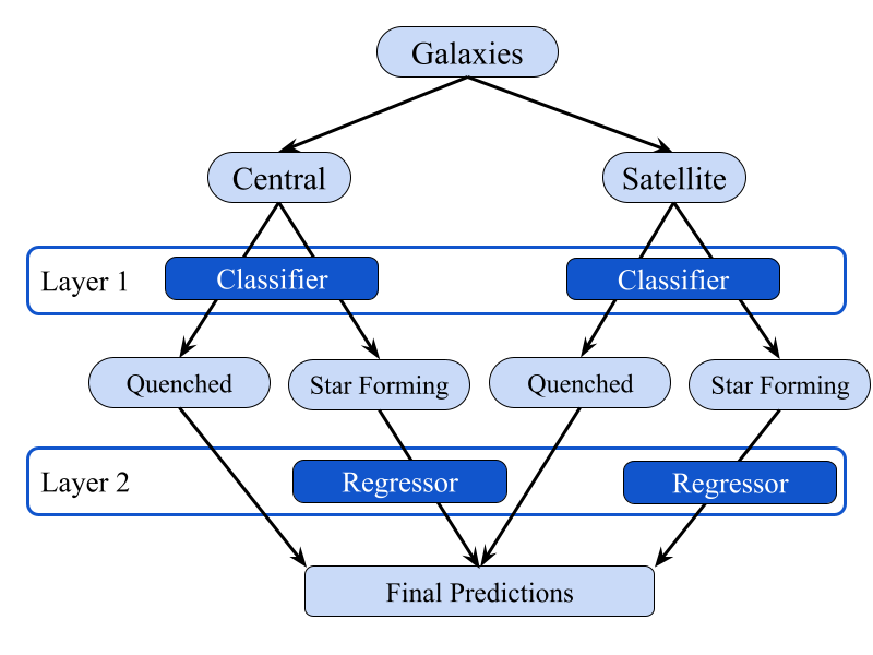
Figure 1: In this flowchart we show the mechanism used in our work. Starting from the top, galaxies are separated into central and satellite subgroups. Following this we introduce ML classifiers at layer 1, to classify each subgroup into SF and Q galaxies, based on the concerned galaxy feature. Subsequently, distinct regressors are employed in layer 2 to independently train on the SF galaxies, encompassing both centrals and satellites. The Q galaxies are assigned a constant value below the SF and Q boundary and merged with the SF predictions to yield the final results.

We introduce a framework to predict various galaxy properties from the halos and subhalos in an N-body simulation, including accounting for the dichotomy between star-forming (SF) and quenched (Q) galaxies. We train and test our ML framework using the Simba simulation. Our framework first separates galaxies into centrals and satellites using the Caesar catalogue as shown in Figure 1. Following this, our framework has two main layers; Layer 1 (darker blue) and Layer 2 (lighter blue). At Layer 1 we introduce ML classifiers to classify both central and satellite galaxies into Q and SF subgroups. After the classification at Layer 2, we introduce ML regressors that independently train on the SF subgroups of central and satellite galaxies. At this stage, a constant value lower than the Q and SF boundary is assigned to all Q galaxies for the concerned features. Ultimately, we merge the predictions from regressors with the constant values assigned to Q, resulting in predictions for all galaxies in the simulation. We explore a large variety of machine learning algorithms, assembling an optimal combination of algorithms for both layers. We then apply this ML framework to an N-body version of the Simba simulation, specifically towards the use case of making predictions for the H i 21cm intensity mapping.

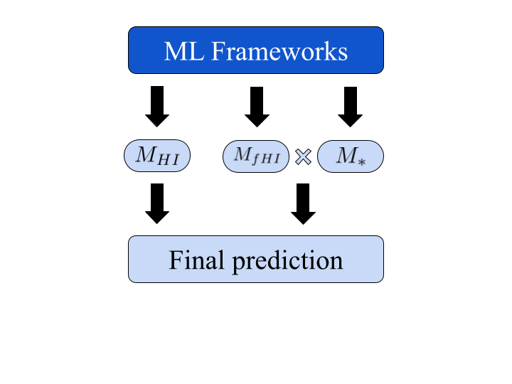
Figure 2: This figure is an illustration of the two approaches we follow to predict the target galaxy features. Here we show the example of $M_{HI}$ prediction. The left half of the figure shows the traditional approach where ML frameworks are trained to predict $M_{HI}$ directly. The right half shows the fraction-based approach, where we train two ML frameworks for $M_{fHI}$ (=$M_{HI}$/$M_{*}$) and $M_{*}$ respectively. Ultimately we multiply them to get back $M_{HI}$ or the main target feature.

Another unique aspect of this work is that we employ data modification to improve accuracy. Various previous works (Lovell et al., 2022; de Santi et al., 2022; Agarwal et al., 2018) have shown the ability of ML algorithms to predict $M_{*}$ accurately. To incorporate this advantage, we divided the other concerned galaxy features with $M_{*}$ and trained ML models to predict these new features. Thus the models are trained to predict the H i fraction ($f_{\rm HI}$)= $M_{\rm HI}$/$M_{*}$, H₂ fraction ($f_{\rm H2}$)= $M_{\rm H2}$/$M_{*}$, and specific star formation rate (sSFR= SFR/$M_{*}$). Then we multiply them with the $M_{*}$ values from the ML framework to recover the desired galaxy features (SFR, $M_{\rm HI}$, and $M_{\rm H2}$) as shown in Figure 2 for $M_{HI}$ predictions. Although this process employs two distinct ML frameworks, the first to predict the fraction and the second to predict $M_{*}$, we show in section 4 that this usually improves the accuracy of the predictions. In all, we develop ML frameworks to predict eight distinct features with different pipelines: $M_{*}$, $M_{\rm HI}$, $f_{\rm HI}$, $M_{\rm H2}$, $f_{\rm H2}$, SFR, sSFR, and metallicity ($Z$).

Ultimately, a key goal of populating galaxies into dark matter halos is accurately determining baryonic mass distributions across the constituent galaxies. This is critical for most science cases, such as creating mock surveys with selection functions or recovering the overall mass within large-scale pixels for intensity mapping. The way to quantify this aspect is via the mass function. However, a common issue with machine learning is that the predicted distribution tends to have a lower width than the true distribution, i.e. ML tends to concentrate predictions toward the mean. This can be problematic for mass functions if the most massive objects are regarded as outliers by the ML and not properly recovered. The significant contribution of these massive objects to the mass budget can sometimes be dominant, thereby skewing the results. To account for this, we have incorporated a post-processing step in our ML pipeline that adds a “ML scatter” to the predictions. This involves the strategic addition of Gaussian noise to better replicate the true extent of the mass function, and thereby more accurately predict the most massive objects that contribute significantly to intensity maps.

In section 2 of this paper, we briefly review the Simba simulation and describe the input and output parameters of our ML frameworks. Our approach on using the ML algorithms and building the frameworks is explained in section 3. section 4 shows our best-performing ML frameworks and a comparison of them with the Simba values. This section also briefly outlines our approach for selecting the optimal algorithms and performance metrics. We also show the applicability of ML-based pipelines at z = 1, 2 through SFR, $M_{\rm HI}$, and $M_{\rm H2}$ predictions in section 6. For each redshift, the mass functions are displayed along with the additional scatter applied to each feature in section 5.

2 THE SIMBA SIMULATION

The Simba simulation is a cosmological hydrodynamic simulation with state-of-the-art galaxy formation modules. It is built on the Gizmo code (Hopkins, 2015), using its meshless finite mass hydrodynamics solved, with the gravity solver mostly taken from Gadget-3 (Springel, 2005). The input physics includes gravity, radiative cooling including metal lines, and on-the-fly self-shielding from a spatially-uniform photo-ionizing background, which directly predicts the H i fraction in each gas particle. Additional processes include star formation based on an on-the-fly subgrid $H_{2}$ the model, stellar feedback using decoupled kinetic winds, black hole growth using both torque-limited and Bondi accretion, black hole feedback in three different modes, and on-the-fly dust production and destruction. Full details of these modules are available in  Davé et al. (2019). This compressive set of input physics generates galaxies and intergalactic gas properties that align very well with a wide range of observations, the most relevant for this work being the gas content of galaxies as a function of mass (Davé et al., 2020) and the quenched fraction of galaxies as a function of mass  Davé et al. (2019). Thus Simba represents a plausible (though not unique) model for the growth and evolution of galaxies from early epochs to today.

The main Simba simulation from the Simba suite, and the one used in the work, is run in a $(100h^{-1}{\rm Mpc})^{3}$ comoving volume, with an adaptive Plummer-equivalent gravitational softening length of $0.5h^{-1}{\rm kpc}$. The gas particle mass resolution is $1.82\times 10^{7}M_{\odot}$, and the dark matter particles have a mass of $9.8\times 10^{7}M_{\odot}$. The assumed cosmology is consistent with Planck+2015, with $\Omega_{m}=0.3$, $\Omega_{\Lambda}=0.7$, $\Omega_{b}=0.048$ $H_{0}=68\;{\rm km}\,{\rm s}^{-1}\;{\rm Mpc}^{-1}$, $\sigma_{8}=0.82$, and $n_{s}=0.97$.

We identify halos on-the-fly with the Friends-of-Friends (FoF) method, incorporated into Gadget-3. Within each halo, galaxies are identified as objects containing stars and dense gas, using a 6D FoF finder incorporated in the Caesar simulation analysis package. Cold gas (H i and $\text{H}_{2}$) is associated with galaxies within each halo as belonging to the galaxy to which it is most bound, thus allowing H i   in particular, to extend beyond the interstellar medium. In this way, Caesar galaxies contain essentially all ($>98\%$) of the H i in the simulated universe at $z\leq 2$. In this work, we employ snapshots 151, 105, and 78 at $z\approx 0,1,2$, respectively. Note that Simba data, including particle snapshots and associated Caesar catalogs containing hundreds of pre-computed properties for each galaxy and halo, is publicly available at simba.roe.ac.uk.

2.1 Halo and Galaxy Properties

We have used the halo and galaxy properties of the Simba 100 Mpc/h box taken from the Caesar catalogs at specific redshifts. The following halo properties were used as input features for the ML frameworks:

• Radii: We employ six radii: one that encloses half (50%) of the dark matter halo mass ($r_{1/2}$), two that contain 20% ($r_{20}$) and 80% ($r_{80}$) of the entire dark matter halo mass. Additionally, three radii are related to the critical density; radii where density reaches 200, 500, and 2500 times the critical density ($R_{200}$, $R_{500}$, $R_{2500}$, respectively). We use $r_{1/2}$ and $R_{500}$ for both central and satellite galaxy predictions; through experimentation, we found it’s best to include $r_{20}$ and $R_{200}$ only for central galaxies, while only using $r_{80}$, $R_{2500}$ values for satellite galaxies.

• Environmental mass density: We use three environmental mass density estimates of Caesar galaxies at various scales, within spherical tophat apertures of 300 kpcs, 1000 kpcs, and 3000 kpcs (comoving).

• Halo spin: We use the dimensionless spin ($\lambda$)(Bullock et al., 2001), defined as:

  $$\lambda=\frac{J_{\mathrm{vir}}}{\sqrt{2}M_{\mathrm{vir}}R_{\mathrm{vir}}V_{\mathrm{vir}}},$$ (1)

  where $J_{\rm vir}$ is the angular momentum within radius $R_{\rm vir}$, $M_{\rm vir}$ is the virial mass, and $V_{\rm vir}=\sqrt{2GM_{\rm vir}/R_{\rm vir}}$ is the halo circular velocity.

• Velocity dispersion: The mass-weighted velocity dispersion for dark matter particles, computed around the center of mass velocity.

• Angular momentum: The magnitude of the specific angular momentum vector (=angular momentum/halo dark matter mass) for the dark matter component of the halo.

• Formation redshift: The redshifts at which the halo accretes 25%, 50%, and 75% of its final mass. For satellite galaxies, we do not include the halo formation redshift as an input feature. This decision is based on our analysis that the halo formation redshift does not have a direct correlation with the growth patterns of satellite galaxies.

For satellite galaxies, we enhance our model’s accuracy by incorporating three specific features that are more relevant to the dynamics of satellite galaxies:

• Subhalo mass: The sum of the mass of all dark matter particles within a 30 kpc (comoving) spherical aperture. This feature can help in understanding the gravitational influence and potential growth trajectory of the subhalo.

• Subhalo velocity: The magnitude of the velocity difference between the subhalo and its host halo. This can provide insights into the dynamical state of the subhalo relative to the center of the halo.

• Subhalo distance: The distance of the subhalo from the center of its host halo. This metric can be crucial for studying the environmental effects on the subhalo.

Incorporating these features significantly enhanced the performance of our models. The impact of these improvements will be quantified using the feature’s importance in section 4.

Our ML frameworks are trained to predict the following galaxy properties from Simba:

• Stellar mass ($M_{*}$): The total mass of all the star particles in a galaxy.

• H i mass ($M_{\rm HI}$): Particle H i fractions are computed on-the-fly assuming a self-shielding model based on Rahmati et al. (2013). A galaxy’s H i mass is the sum of all H i in particles that are most bound to it within its halo.

• $\text{H}_{2}$ mass ($M_{\rm H2}$): Particle $\text{H}_{2}$ fractions are computed on-the-fly using a subgrid model based on Krumholz & Gnedin (2011). The $\text{H}_{2}$ mass of a galaxy is computed analogously to the H i mass.

• Star formation rate (SFR): Particle SFRs are computed from the $\text{H}_{2}$ density divided by the local dynamical time, times an efficiency of 0.02. The total SFR is the sum of individual particle SFRs within a galaxy.

• Metallicities (Z): We used two types of metallicities; SFR-weighted and $M_{*}$ weighted. Our goal is to predict the SFR-weighted metallicity, but for galaxies without SFR values (generally old galaxies), we predict the $M_{*}$ weighted metallicity values, as every galaxy has stellar mass. In general, the difference between the SFR-weighted and mass-weighted Z is small.

3 MACHINE LEARNING SETUP

Galaxies are categorized into diverse populations, each characterized by distinct attributes. Among these classifications, galaxies are differentiated into central and satellite categories, reflecting their positional dynamics within cosmic structures. Furthermore, galaxies are distinguished based on their stellar activity, identified as Star-Forming (SF) or Quiescent (Q) galaxies. This bifurcation enables the creation of four specific subgroups: Central-SF, Central-Q, Satellite-SF, and Satellite-Q. As highlighted in section 1, existing Machine Learning (ML) frameworks have predominantly focused on analyzing the Central-SF subgroup or if fitting anything, have struggled to distinguish between these groups effectively.

In the Caesar catalog, the galaxy with the highest stellar mass ($M_{*}$) within a halo is designated as the central galaxy, while all remaining galaxies are classified as satellites. This delineation allows for the straightforward categorization into central and satellite sub-populations. To differentiate between Star-Forming (SF) and Quiescent (Q) galaxies, we adhere to the methodology outlined in Andrianomena et al. (2020), employing a Machine Learning (ML) classifier for this purpose. However, unlike them, we train our classifiers on the sSFR boundaries taken from (Davé et al., 2019) as:

$$\mathrm{sSFR}=10^{-1.8+0.3z}\mathrm{Gyr}^{-1}$$ (2)

Where z is the redshift. Subsequently, we train the ML classifier on this boundary based on the halo’s attributes at redshifts 0, 1, and 2. This approach has enabled us to automate the identification of central/satellite and SF/Q galaxies from a collection of halos, complete with recognized subhalos. Consequently, the classification of galaxies into the four distinct subgroups is seamlessly integrated into our pipeline.

For the Q galaxies, we assume they have negligible SFR, $M_{\rm HI}$, and $M_{\rm H2}$. This assumption generally holds in Simba; the SF galaxy population retains 80.3%, 85.7%, and 83.7% of the overall SFR, $M_{\rm HI}$, and $M_{\rm H2}$ respectively at $z=0$. For higher redshifts, for $M_{\rm HI}$, the SF population share at $z=1$ is 94.8%, and at $z=2$ is 98.0%. Thus, in terms of large-scale observables such as intensity mapping, the Q population adds a minor or small contribution that we will ignore. We leave it for future work to correct for the gas and SFR contributions from Q galaxies. Our pipelines will automatically output the values of the Q galaxy features as a constant value, lower than the SF/Q boundary.

For $M_{*}$, our approach deviates slightly from the previously described framework. While we continue to utilize the Caesar catalog for segregating galaxies into central and satellite categories, the application of ML classifiers to distinguish between SF and Q galaxies is not required in this context. This exception arises because the demarcation between Q and SF populations based on $M_{*}$ is not as pronounced as it is for other features. Therefore, for $M_{*}$, we directly implement a regressor model for central and satellite galaxies focusing on predicting $M_{*}$ without the need to pre-classify galaxies into SF or Q categories.

For the SF galaxies, we train ML regressors to learn the relation among halo and galaxy features separately for centrals and satellites. The training, testing, and optimization of these regressors are conducted for each subgroup and ultimately consolidated into a cohesive model.

In the subsequent sections, we describe the specifics of the ML algorithms employed for both classification and regression tasks. A key aspect of these algorithms is the presence of adjustable parameters known as "hyperparameters". Adjusting these parameters allows for the customization of the model to meet our specific objectives. Manual tuning of these hyperparameters designates the algorithms as "hand-tuned". This manual tuning process, while offering precise control, can be labor-intensive and complex. To address this, we also explore several automated ML algorithms. These automated approaches facilitate the comparison of different ML algorithms by autonomously adjusting their hyperparameters, thereby optimizing them based on a predetermined criterion. Upon completing this comparative analysis, we assess the accuracy metrics of each method. This evaluation enables us to integrate the strengths of each approach, culminating in the derivation of the most effective ML algorithms, complemented by optimally tailored sets of hyperparameters.

3.1 Hand-Tuned Machine Learning Algorithms

3.1.1 Random Forest (RF)

RF is a decision tree-based algorithm renowned for its effectiveness in handling datasets with multiple features. It is versatile, and capable of operating both as a regressor and a classifier, making it ideally suited for our dual purposes: classifying galaxies into SF/Q categories and performing regression analyses within the SF galaxy population. In the regression context, the RF model predicts an output based on the mean value derived from the ensemble of decision trees. Conversely, when functioning as a classifier, it determines the outcome through a majority vote among the trees. This method of using ensemble averages or majority voting enables the RF algorithm to bypass the selection of individual decision trees, which may be prone to overfitting, thereby enhancing the robustness and reliability of our model.

We utilize the Random Forest regressor and classifier implementations from the Scikit-Learn Python library. The hyperparameters n_estimators, max_features, and bootstrap were specifically tuned via a grid search, while the remaining parameters were kept at their default settings as specified by the library.

3.1.2 Support Vector Machine (SVM)

The Support Vector Machine classification algorithm is designed to optimize a hyperplane that effectively separates the target variable into distinct categories. Similarly, Support Vector Regression (SVR) adheres to a comparable principle but aims to identify the optimal surface that best represents the desired feature, rather than categorizing data points. The critical aspect of both SVM and SVR is the flexibility in choosing the nature of the hyperplane be it linear or nonlinear based on the specific requirements of the dataset and the task at hand.

We have used the publicly available SVM and SVR functions from the Scikit-Learn Python library. The hyperparameters C and gamma were tuned via a grid search and the remaining parameters were maintained at their default settings as established by the library.

3.1.3 k-Nearest Neighbours (kNN)

The k-Nearest Neighbors algorithm represents a straightforward, non-parametric approach to both regression and classification tasks. The parameter $k$, signifying the number of nearest neighbors to consider, plays a crucial role in the algorithm’s performance and can be finely adjusted to enhance the outcome. In essence, the algorithm categorizes a query point by identifying the $k$ closest neighbors, with proximity measured by the minimum Euclidean distance. For regression tasks, the kNN regressor computes the output as the average value of the attributes of the $k$ nearest neighbors. We have implemented this algorithm using the KNeighborsClassifier and KNeighborsRegressor from the Scikit-Learn Python libraries.

We have implemented this algorithm using the KNeighborsClassifier and KNeighborsRegressor from the Scikit-Learn Python library. To optimize the algorithm’s performance, n_neighbors, weights, and metric hyperparameters were tuned via a grid search and the remaining were maintained at their default settings as established by the library.

3.2 Automated Machine Learning (AutoML) Algorithms

3.2.1 Tree-based Pipeline Optimization Tool (TPOT)

TPOT (Olson et al., 2016) stands out as a distinguished AutoML algorithm. We have incorporated TPOT’s publicly available Python library into our research framework. TPOT leverages the robust Scikit-Learn library to handle data and access a comprehensive suite of machine learning algorithms. Fundamentally, TPOT employs Genetic Programming, a stochastic global search technique, a method that autonomously explores a vast space of potential machine learning pipelines to find the top-performing ML model for the concerned dataset.

3.2.2 AutoSklearn

AutoSklearn (Feurer et al., 2015) is another open-source AutoML library designed for Python that harnesses the Scikit-Learn framework for data processing and the implementation of machine learning algorithms. Diverging from the genetic programming approach of TPOT, AutoSklearn employs Bayesian Optimization to navigate the search space of machine learning pipeline configurations. This method focuses on efficiently identifying the most promising model architectures and hyperparameter settings by learning from the performance of previously evaluated configurations. Bayesian Optimization aims to balance the exploration of new models against the exploitation of models known to perform well, thereby finding the optimal ML pipeline for a given dataset.

3.2.3 AutoKeras

AutoKeras (Jin et al., 2019) is an innovative AutoML framework built atop Keras, focusing specifically on the automation of parameter optimization for Artificial Neural Networks (ANNs). ANNs are complex structures composed of interconnected neurons or nodes organized into layers, where each neuron in one layer is linked to every neuron in the subsequent layer via activation functions. These connections are weighted, and the optimization of these weights is crucial, as it minimizes the discrepancy between the predicted and actual values during the training phase. AutoKeras simplifies the intricate process of determining the most effective model architecture and the associated hyperparameters, known as neural architecture search. To achieve this, AutoKeras employs Bayesian Optimization and Gaussian Processes that systematically explore the architecture and parameter space.

3.3 Voting

Voting isn’t an ML algorithm itself, but an ensemble technique that combines outputs from other well-performing algorithms. For the classifier, we collect votes among the algorithms for a given data point to predict its class. For the regressor, we compute the average of the predictions from different ML algorithms. In our study, we have applied the Voting technique by integrating both Hand-Tuned and Automated ML algorithms, selecting the top three performers as contributors to the ensemble.

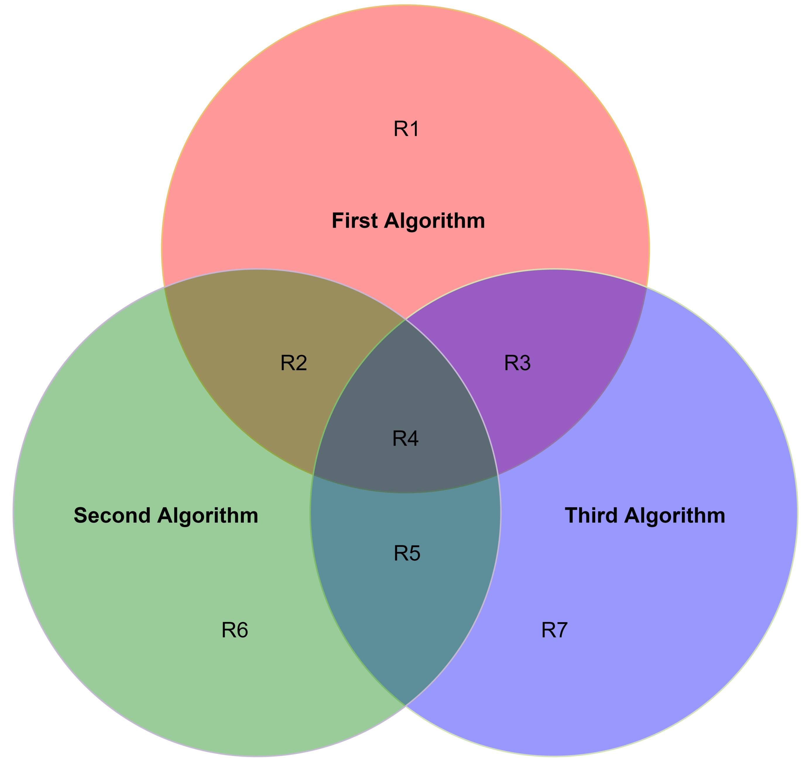
Figure 3: This figure shows the Voting mechanism for classifiers, among three algorithms; First Algorithm (red), Second Algorithm (green), and Third Algorithm (blue) through a Venn diagram, on the test dataset. R1, R2, R3, R4, R5, R6, and R7 depict different groups of galaxies depending on predictions from the algorithms.

We will explain the voting mechanism for classifiers through the Venn diagram in Figure 3. Assume the circle corresponding to each algorithm contains the galaxies they predicted to be Q. Depending on the commonality of results among the algorithms, we have seven groups: R1, R2, R3, R4, R5, R6 and R7. Our Voting method predicts a galaxy to be Q if any two (or three) of the algorithms predict the galaxy to be quenched. Possible groups that result from this are R1+R2+R3+R4+R5+R6 (First and Second algorithm), R2+R3+R4+R5+R6+R7 (Second and Third algorithm), R7+R5+R4+R3+R1+R2 (Third and First algorithm), and all groups combined (All three algorithms).

In the case of regressors, for a given feature, Voting predicts the average value of predictions given by at least two best-performing regressor algorithms. Being an ensemble technique, Voting helps in reducing the overfitting issue by smoothing out individual errors and biases inherent in individual models.

3.4 Classifier

The aim is to determine whether a galaxy is SF or Q based on sSFR. The dataset is initially split into central and satellite subgroups. At $z=0$ Simba 100 Mpc/h box contains 35843 central and 19766 satellite galaxies; at $z=1$, it has 27198 central galaxies and 12100 satellite galaxies; and at $z=2$, it has 23042 central galaxies and 7701 satellite galaxies. Then we divide both the subgroups at each redshift into two parts; training and testing samples, in a 4:1 ratio. We begin by constructing various classifiers, as listed in previous subsections, which are trained on the training sample and later tested on the testing sample using the parameters derived from the confusion matrix presented below.

3.4.1 Confusion Matrix

A confusion matrix is used to describe the performance of a classifier. In our case of distinguishing between two classes considered as positive (SF) and negative (Q), the classification yields four possible outcomes:

• True Positive (TP): Correct prediction of the positive class.

• True Negative (TN): Correct prediction of the negative class.

• False Positive (FP): Incorrect prediction of the positive class.

• False Negative (FN): Incorrect prediction of the negative class.

Several metrics derived from these outcomes are employed to quantify the performance, notably True Positive Rate (TPR), Positive Predictive Value (PPV), True Negative Rate (TNR), and Negative Predictive Value (NPV), which are defined as:

$$TPR=\frac{TP}{TP+FN},\hskip 36.135ptPPV=\frac{TP}{TP+FP},$$ (3)

$$TNR=\frac{TN}{TN+FP},\hskip 36.135ptNPV=\frac{TN}{TN+FN}.$$ (4)

Given the predominance of SF galaxies (positive class) over Q galaxies (negative class) in the Simba dataset, a high degree of accuracy in predicting the positive class is anticipated due to their substantial representation in the training data. Our paper’s primary objective is to ensure Q galaxies are accurately accounted for in the ML predictions. As such, prioritizing the maximization of the Negative Predictive Value (NPV) aligns with our goal, as a high NPV indicates a model’s efficacy in correctly identifying Q galaxies. Consequently, the classifier demonstrating the highest NPV will be deemed the most appropriate for our framework ensuring precise and balanced classification of SF and Q galaxies.

3.5 Regressor

In the previous subsection, we explained the methodology for identifying the most effective classifiers for each of the seven galaxy features. Here, we will develop regressor models for the SF subgroup of these features, as well as for $M_{*}$. We start by using the top-performing classifiers to initially sort the entire dataset into SF and Q galaxies. Due to the inherent imperfections of these classifiers, resulting in some Q galaxies being misclassified as SF and vice versa, we aim to enhance the regressor models’ resilience. To achieve this, galaxies that are SF but were misclassified as Q are included in the training dataset for the regressors. This augmented dataset of SF galaxies identified both manually and through ML classification is then utilized to train the regressor models. The performance of each regressor is subsequently assessed on the subset of SF galaxies identified solely through ML classification.

Now, we introduce several straightforward yet widely utilized methods for assessing the accuracy of regressor models. Initially, we visualize the relationship between predicted and true values by plotting the former against the latter for the test dataset. For a model with perfect accuracy, all data points on the scatter plot would align with the $y=x$ line, indicating a one-to-one correspondence between true and predicted values. Deviations from this ideal are represented by points scattering around the $y=x$ line, with $y\neq x$.

To quantitatively measure these deviations, we compute four key parameters, analogous to Agarwal et al. (2018): mean deviation ($\mu$), root mean square (RMS) width ($\sigma$), regression score ($R^{2}$), and the Pearson correlation coefficient ($\rho$). Please note that unlike the method in Agarwal et al. (2018), we calculate the absolute mean deviation. The mathematical formulations for these metrics, considering $x_{i}$ and $\hat{x}_{i}$ as the logarithms of the true and predicted values for the $i^{th}$ data point in a sample of size $N$, are given as follows:

$$\mu(x,\hat{x})=\frac{1}{N}\sum_{i}^{N}\left|x_{i}-\hat{x}_{i}\right|$$ (5)

$$\sigma^{2}(x,\hat{x})=\frac{1}{N-1}\sum_{i}^{N}\left[\left|x_{i}-\hat{x}_{i}\right|-\mu\right]^{2}$$ (6)

$$R^{2}(x,\hat{x})=1-\frac{\sum_{i}^{N}\left[x_{i}-\hat{x}_{i}\right]^{2}}{\sum_{i}^{N}\left[x_{i}-<x>\right]^{2}}$$ (7)

$$\rho(x,\hat{x})=\frac{\sum_{i}^{N}\left(x_{i}-<x>\right)\left(\hat{x}_{i}-<\hat{x}>\right)}{\sqrt{\sum_{i}^{N}\left(x_{i}-<x>\right)^{2}}\sqrt{\sum_{i}^{N}\left(\hat{x}_{i}-<\hat{x}>\right)^{2}}},$$ (8)

where $<x>=\sum_{i}^{N}x_{i}/N$ and $<\hat{x}>=\sum_{i}^{N}\hat{x}_{i}/N$. These metrics are computed for all ML algorithms discussed in the previous section to understand the model accuracy comprehensively. Ultimately, the algorithm demonstrating the lowest $\sigma$ value is selected as the most suitable for our framework.

3.6 The Final ML Framework

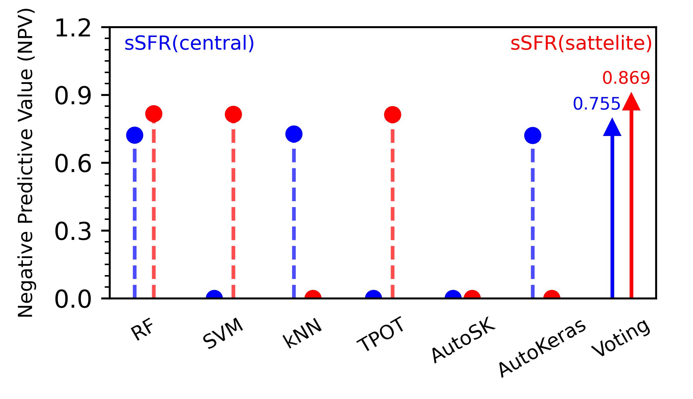
Figure 4: Best performing sSFR-based classifier models for central (blue) and satellite galaxies (red) at $z=0$. The models having the highest $NPV$ value for each feature is denoted by the triangle at the head with the corresponding $NPV$ value mentioned just above it. If Voting is the best performing algorithm, the participating algorithms are plotted with dotted lines and a circle on the top.

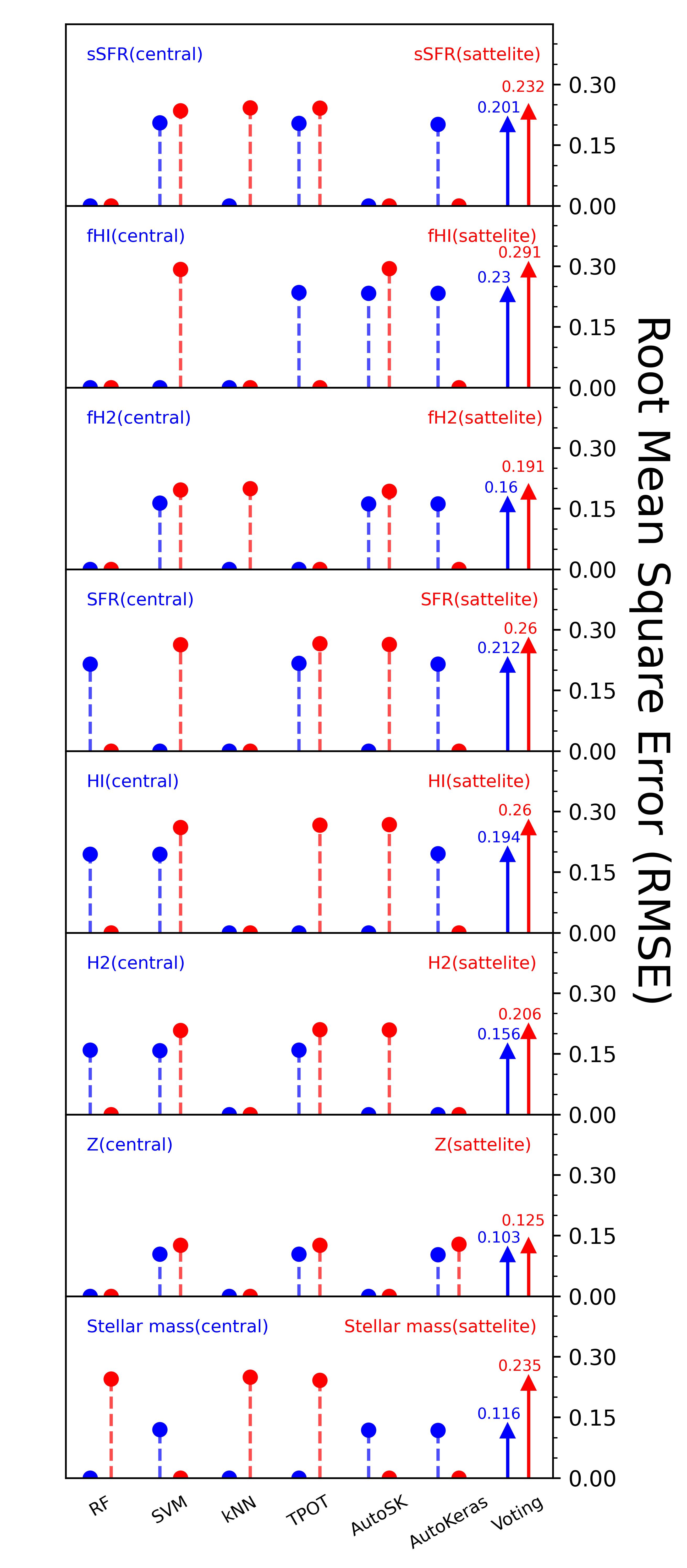
Figure 5: Feature wise best performing regressor models for central (blue) and satellite galaxies (red) at $z=0$. Models with the lowest $\sigma$ value for each feature is denoted by the triangle at the head with the corresponding with the $\sigma$ value presented above. If Voting is the best performing algorithm, the participating algorithms are plotted with dotted lines and a circle on the top.

The first half of our ML framework is a classifier to determine whether the galaxy is Q or SF, and the second half is a regressor. Both Hand-Tuned ML and AutoML algorithms have been trained for all the features. Results from the Hand-Tuned algorithms were further optimized by modifying a few of their hyperparameters via a grid search as mentioned in subsection 3.1.

Figure 4 shows the best-performing classifiers and Figure 5 shows the best-performing regressors for our optimal parameter choices of each algorithm. The blue bars represent the results for central galaxies, while the red bars are for satellite galaxies. In the case of classifiers, we focus on the NPV. Conversely, for regressors, we highlight the algorithms that achieve the minimum RMSE. The bar with an arrow at its top identifies the algorithm of choice for the corresponding feature, with the exact value of NPV or RMSE displayed above this arrow.

We discuss the classifier and regressor models and their performance in the subsequent section, providing a detailed analysis of each feature.

4 The accuracy of the ML frameworks

In this section, we present the best-performing ML frameworks for each feature under consideration and provide a comparative analysis between the predictions generated by these frameworks and the actual values derived from the Simba simulation. To illustrate ML accuracy, it is conventional to construct scatter plots showing true versus predicted values for each galaxy. However, when considering attributes related to star formation and gas content, galaxies identified as Q typically register significantly lower values than their SF counterparts. In scenarios where the focus lies on ensemble quantities such as intensity mapping, Q galaxies do not significantly influence the evaluation of the model’s predictive accuracy. For instance, within the Simba simulation at $z=0$, the Q galaxy population contributes to less than 1% of the total SFR, H i, and $\text{H}_{2}$ across the entire volume. Consequently, our analysis of ML efficacy in populating galaxy properties into halos will focus primarily on the regressor models’ performance, given the effective functioning of the classifier in distinguishing between SF and Q galaxies.

This section also introduces several scatter plots that illustrate the true versus ML-predicted values for various properties from Simba. Notably, these plots will selectively feature galaxies that are classified as SF by both the ML models and the Simba simulation. For the sake of completeness, we explain the methodology behind the construction of such plots in Appendix A.

Figure 6 illustrates the accuracy of our ML model predictions, plotted on the y-axis, in comparison to the actual values derived from the Simba simulation, plotted along the x-axis, for each concerned galaxy feature. Each point on the plot represents an individual galaxy, providing a granular view of the model’s predictive accuracy. Ideally, a perfectly predicted value would align with the diagonal red line, indicating a one-to-one correspondence between the predicted and true values. The plot employs color coding to represent probability densities, which enhances the visual differentiation of data concentration across the plot. In regions of lower density, individual galaxies are depicted in black, enhancing clarity in areas where the data points are more dispersed.

Key metrics that quantify the fit’s quality are displayed in the plot’s upper left corner including the $1\sigma$ scatter $\sigma$, mean square error $\mu$, the regression score $R^{2}$, and the Pearson correlation coefficient $\rho$. Additionally, we introduce a parameter, denoted as $\%OB$, to these scatter plots. This parameter addresses the issue of misclassifications by the classifier, which often predicts values significantly lower than the SF-Q threshold for the respective parameters. Incorporating all data points in the plot tends to dilute the focus on high-density regions by broadening the plot boundaries. To counteract this and better highlight the high-density areas, we adjust the scatter plot boundaries and designate outliers, typically constituting less than 1% of the SF subgroup, to the plot’s boundaries. The $\%OB$ parameter quantifies the percentage of such outliers within the total dataset represented in the plot, providing a measure of the extent to which these outliers influence the overall data visualization.

In the following subsections, we discuss each the choice of regressor (Figure 5) for each feature and the fitting accuracy (Figure 6) at $z=0$.

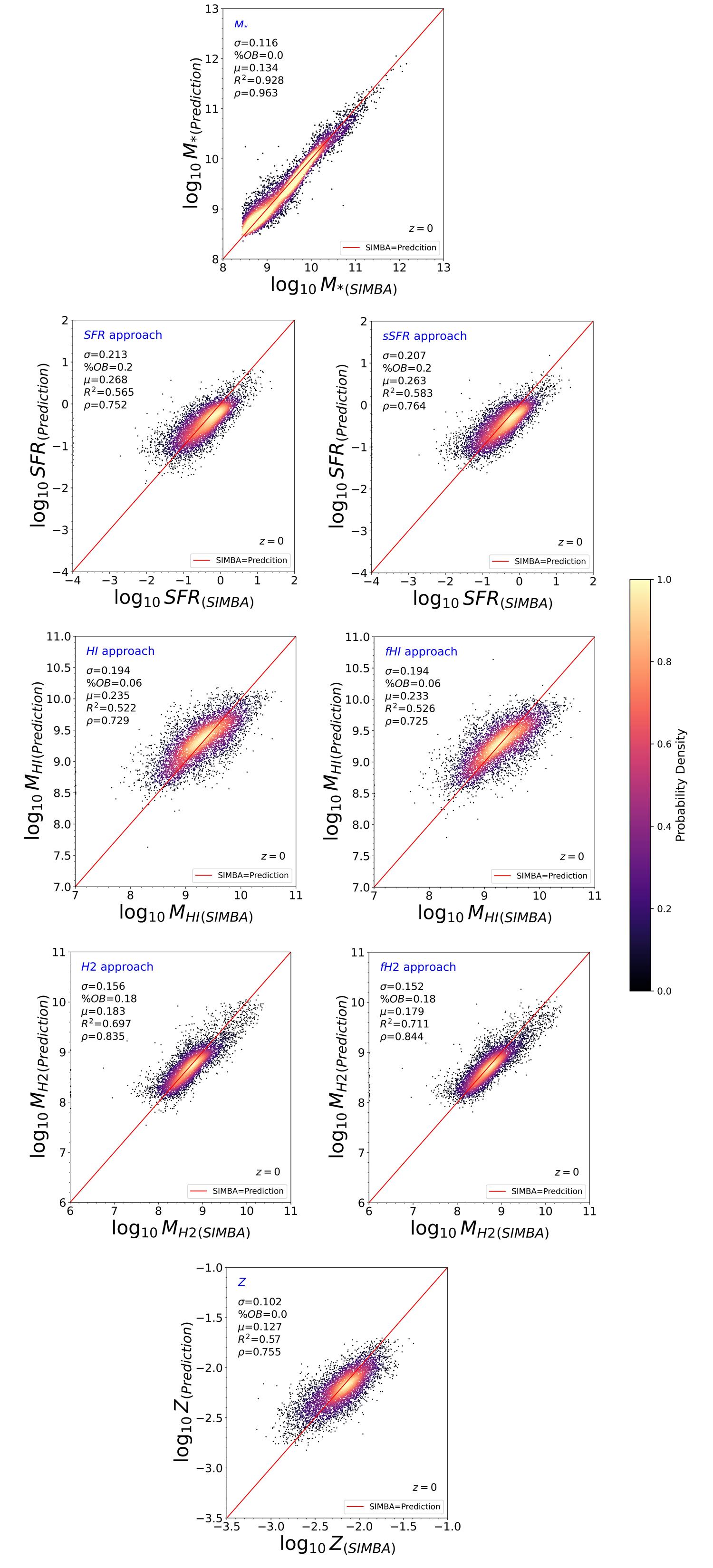
(a) Central Galaxies

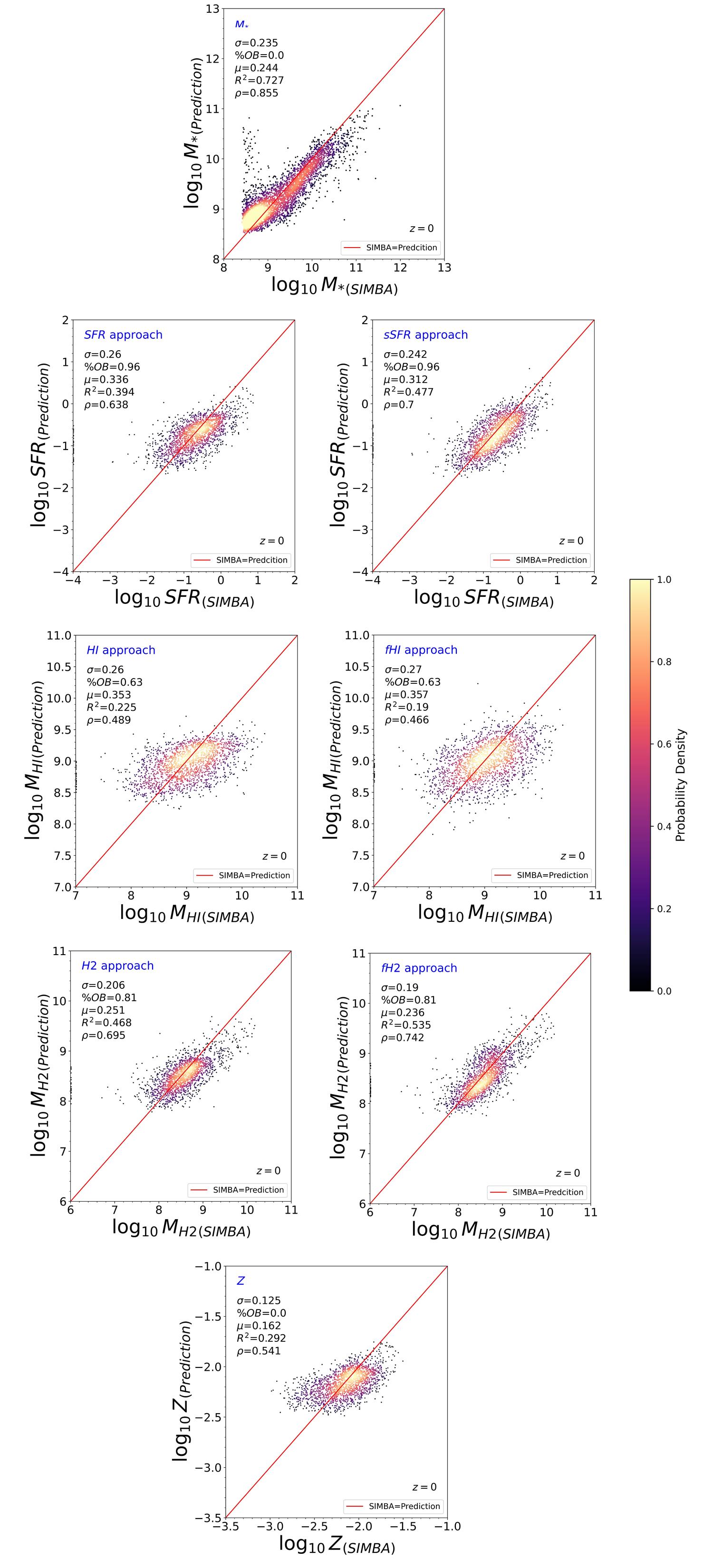
(b) Satellite Galaxies

Figure 6: Prediction accuracy for the best-performing frameworks for fractions-based and feature-based approaches using Simba simulation at $z=0$. The scatter plots have the true (Simba) values on the x-axis, while the y-axis has the predicted values. (a) has ML predictions related to central galaxies and (b) has ML predictions related to satellite galaxies.

4.1 Stellar mass $M_{*}$

Stellar mass is generally closely correlated with halo mass, in both observations (More, 2011) and simulations with the scatter correlated with halo properties (Cui et al., 2021). Thus it is unsurprising that ML frameworks have generally had success reproducing $M_{*}$ from dark matter properties (Kamdar et al., 2016; Agarwal et al., 2018). Our ML framework produces similarly good results, but here we further delineate in terms of centrals vs. satellites. As we mentioned earlier $M_{*}$ doesn’t need a classifier to separate SF from Q galaxies.

For $M_{*}$, the Voting method, which aggregates outputs from SVM, AutoSklearn, and AutoKeras for central galaxies, and RF, kNN, and TPOT for satellite galaxies, yielded the lowest $\sigma$ values for both galaxy types (refer to the bottom panel in Figure 5). For central galaxies, the Root Mean Square Error (RMSE) is notably low $\sigma=0.116$, accompanied by an impressive Pearson correlation coefficient $\rho=0.963$, as shown in the top panel of 6(a). This highlights the efficacy of ML in accurately estimating the stellar masses of central galaxies, supporting findings from previous studies and this holds throughout the mass range probed with Simba.

Conversely, the prediction of $M_{*}$ for satellite galaxies is less precise, with a $\sigma$ value of 0.235 and a greater incidence of significant outliers, especially at lower $M_{*}$ values (illustrated in the top panel of 6(b)). This is because the overall dark matter halo properties are primarily connected to the central galaxy, but the satellites can experience various effects that confuse their own dark matter halo with that of the overall parent halo, thereby reducing the effectiveness of reconstruction from the dark matter. Still, the overall predictions are reasonably good, with the mean square error $\mu\sim 0.24$ dex and a Pearson coefficient of 0.86.

In summary, our analysis confirms that $M_{*}$ can be reliably inferred from DM properties using our ML framework. While the correlation for central galaxies aligns with expectations given their direct association with halo growth, the framework’s applicability extends to satellite galaxies, especially when incorporating satellite-specific DM information like 3-D aperture mass and proximity to the central galaxy. Further discussion on feature importance will follow later on.

4.2 Star formation rate SFR

SFR has historically been more challenging to predict from dark matter features in simulations using ML (Agarwal et al., 2018; Jo & Kim, 2019). Unlike $M_{*}$ which is a cumulative quantity and therefore mostly grows (modulo stellar mass loss and satellite stripping), the SFR can fluctuate both up and down, on timescales significantly shorter than halo dynamical times owing to local processes such as stochastic gas accretion and internal dynamical evolution. Additionally, satellites can suffer environmental quenching processes that may not have direct correlations with dark matter. Yet predicting SFRs is crucial for connecting N-body predictions with, for instance, emission line surveys. Here we examine the performance of our ML framework for predicting SFR.

Unlike the prediction of stellar mass $M_{*}$, SFR, along with $M_{\rm HI}$, and $M_{\rm H2}$, requires a preclassifier, depicted in the classifier layer of Figure 1. This step sets a specific boundary for sSFR given by Equation 2, which simplifies to $10^{-10.8}$$yr^{-1}$ for $z=0$. Now we proceed to train various models as outlined in subsection 3.4.

In the process of classifying galaxies, the Voting method, which aggregates predictions from three ML models, yielded the highest NPV for both central and satellite galaxies as shown in Figure 4. For central galaxies, a galaxy is classified as Q by Voting if either RF, kNN, or the model from AutoKeras indicates the galaxy to be Q. For satellite galaxies, Voting classifies a galaxy to be Q when either RF, SVM, or the model from TPOT identifies it as such.

The classifier has demonstrated significant efficiency in segregating Q from SF galaxies across both central and satellite populations. Specifically, central galaxies exhibit a NPV of 0.76, while satellites present an even more robust NPV of 0.87. This enhanced performance among satellite galaxies is likely attributable to a substantial proportion of Q galaxies within this subgroup. Conversely, the central galaxy population predominantly consists of SF galaxies, where even a modest number of misclassifications can lead to a significant number of FN, resulting in a lower TN, and consequently, a more fluctuating and generally lower NPV. The other performance metrics for central galaxies remain commendable as well; $TPR=0.95$, $PPV=0.94$, and $TNR=0.71$. However, these metrics were less impressive yet decent for satellites; $TPR=0.82$, $PPV=0.72$, and $TNR=0.79$. The variance in TNR values has a similar explanation to NPV. However, the change in TPR and PPV stems from the dominant presence of SF galaxies within the central galaxy training dataset, as opposed to satellites. Consequently, ML models for central galaxies predict SF galaxies more proficiently than for satellites.

A key takeout from here can be the importance of $NPV$ and $TNR$, since they are more prone to fluctuations with the model accuracy, to predict the negative class in particular. The variance in TN is more conspicuously mirrored in these metrics, with $NPV$ focusing more on the negative class. Given our objective to precisely predict Q galaxies (the negative class), $NPV$ emerges as the most conservative way to choose the best algorithm.

With our classifier in place, we can examine the regressor performance, shown in Figure 6 (a, b), second row left panels. In this configuration, galaxies classified as Q by the classifier are assigned a nominal SFR of $10^{-5}$$yr^{-1}$, while the SFR for SF galaxies is determined by the regressor models, with results depicted in the fourth row of Figure 5. Although the regressor predictions do not achieve the same level of accuracy as those for $M_{*}$, they mark a notable improvement over previous studies. The $\sigma$ of the predictions is recorded at 0.21 for central galaxies and 0.26 for satellites, with Pearson correlation coefficients ($\rho$) of 0.75 and 0.76, respectively. A significant observation is the lack of bias in the ML framework towards central galaxies; the data points align closely with the 1:1 relation, albeit with some scatter. This alignment is critical as it suggests that aggregating the SFR predictions across multiple galaxies could effectively reduce the uncertainty in these estimates, thus enhancing the robustness of the overall prediction. However, it is noteworthy that for satellite galaxies, there is a visible trend of underprediction at higher SFR values, highlighting a potential area for further refinement in our ML models.

An alternative strategy for predicting SFR employed in this study is the fraction-based method. This approach involves estimating the sSFR through ML algorithms and subsequently multiplying it by the ML-predicted $M_{*}$ to derive the SFR. As previously noted, the classifier outcomes derived from the Voting method yield the highest NPV for both central and satellite galaxies. For central galaxies, a galaxy is classified as Q by Voting if either RF, kNN, or the model from AutoKeras indicates the galaxy to be Q. For satellite galaxies, Voting classifies a galaxy to be Q when either RF, SVM, or the model from TPOT identifies it as such.

In the second layer of our framework, Q galaxies identified by the classifier were assigned an sSFR of $10^{-15}$$yr^{-1}$. The sSFR for SF galaxies were estimated using regressor models, as shown in the top panel of Figure 5. These sSFR estimates were then multiplied by the corresponding $M_{*}$ predictions from subsection 4.1 to calculate SFR. The comprehensive predictions are visualized in the second-row right panel of Figure 6(a, b). For central galaxies, the $\sigma$ value from the sSFR method 0.207 showed a slight improvement over the direct SFR method 0.213, with a corresponding increase in the Pearson coefficient from 0.75 to 0.76. For satellite galaxies, the adoption of the sSFR-based prediction method improved $\sigma$ from 0.26, when using the direct SFR prediction method, to 0.24 with the sSFR approach. More significantly, the Pearson correlation coefficient experienced a substantial increase, moving from 0.64 in the SFR prediction model to 0.7 in the sSFR-based framework.

The results from Figure 6(b) indicate a more symmetrical distribution of predictions around the $y=x$ line using the sSFR approach compared to the traditional method, likely leading to the improved correlation coefficient. Additionally, Figure 6(a) reveals that outliers or points significantly diverging from true values, exhibit greater scatter in the SFR approach. Thus, the fraction-based approach notably excels over the traditional feature-based method in predicting SFR, evidenced by its higher accuracy and more uniform prediction distribution.

4.3 $M_{\rm HI}$

The prediction of $M_{\rm HI}$ from halo features has received significant attention in the realm of ML applications to cosmology. This interest stems from the important role of $M_{\rm HI}$ in understanding galaxy formation and evolution, as well as in mapping the large-scale structure of the universe through 21cm emission line surveys. Here, we outline the pipelines developed for $M_{\rm HI}$ predictions within our ML framework and evaluate the accuracies achieved.

Just like SFR, the prediction of $M_{\rm HI}$ begins with a preclassifier to separate SF and Q galaxies, establishing a two-layer ML model framework for both central and satellite galaxies. The classifiers, detailed in subsection 4.2 and illustrated in Figure 4, are applied to the dataset.

Subsequently, Q galaxies identified by the classifier are attributed a nominal $M_{\rm HI}$ value of $10^{2}M_{\odot}$, and the $M_{\rm HI}$ for SF galaxies is predicted using regressor models, as shown in the fifth row of Figure 5. The predictions, as presented in the third-row left panel of Figure 6(a, b) have quite favorable $\sigma$ value of 0.19 for central galaxies which slightly rises to 0.26 for satellite galaxies. Importantly, similar to SFR predictions, the ML framework here exhibits an unbiased approach with no evident shift towards either side of the 1:1 relation, ensuring an even-handed distribution across galaxy types.

We now turn our attention to the implementation of the fraction-based approach within our machine learning framework. This method entails the prediction of $M_{fHI}$ followed by its multiplication by the ML-predicted $M_{*}$ to derive $M_{\rm HI}$ values. The initial step involves the application of classifiers to segregate the dataset into relevant categories, as previously outlined in subsection 4.2 and visually represented in Figure 4.

In the subsequent phase of our fraction-based approach, galaxies classified as Q were assigned a nominal $M_{fHI}$ of $10^{-10}$, and the SF counterparts were estimated using regressor models, as shown in the second from the top panel of Figure 5. These $M_{fHI}$ predictions were then multiplied by the corresponding $M_{*}$ estimates, as discussed in subsection 4.1, to calculate $M_{\rm HI}$ values. The final predictions are illustrated in the third-row right panel of Figure 6(a, b).

For central galaxies, the standard deviation $\sigma$ remains consistent at 0.19 across both methodologies. However, for satellite galaxies, the $\sigma$ values exhibit slight variation, recorded at 0.27 for the $M_{fHI}$ approach and 0.26 for the direct $M_{\rm HI}$ prediction. Visual inspection of Figure 6(a) reveals a tighter spread for the $M_{fHI}$ method, especially in the plot’s central region, where the dense yellow area appears slightly more centralized towards the fraction-based approach. Figure 6(b) indicates that despite a marginally increased scatter of outliers in the fraction-based method, it suffers less from underprediction at higher masses compared to the direct $M_{\rm HI}$ approach for satellite galaxies. Thus, while statistical metrics suggest similar predictive performance for both methods, the visual analysis provides a nuanced advantage to the fraction-based approach in accurately predicting $M_{\rm HI}$ values.

4.4 $M_{\rm H2}$

While the prediction of $M_{\rm H2}$ using ML has not garnered as much attention as $M_{\rm HI}$ predictions, it remains a crucial element for comprehensive gas and baryonic content estimation within galaxies, and will become increasingly important as CO line emission surveys for cosmology emerge (Keating et al., 2020). The following sections outline the pipelines developed for $M_{\rm H2}$ predictions within our ML framework and assess the accuracies achieved.

Similar to the methodology adopted for SFR and $M_{\rm HI}$ predictions, the estimation of $M_{\rm H2}$ commences with the application of a preclassifier to separate SF from Q galaxies. This preliminary step lays the groundwork for a dual-layer ML model framework similar to that used for SFR and $M_{\rm HI}$ predictions, applicable to both central and satellite galaxies. The classifiers elaborated in subsection 4.2 and visually represented in Figure 4 are applied to the dataset for subsequent analysis.

Following the classification step, galaxies identified as Q by the classifier were assigned a nominal $(M_{\rm H2}$ value of $10^{4}M_{\odot}$. The $M_{\rm H2}$ for SF galaxies was then estimated using regressor models, as outlined in the sixth row of Figure 5. The performance of these predictions is highlighted in the fourth-row left panel of Figure 6(a, b), demonstrating notable accuracy with mean deviation $\sigma$ values of 0.16 for central galaxies and 0.21 for satellite galaxies. Furthermore, the Pearson correlation coefficient for both central and satellite galaxies is decent, recorded at 0.84 and 0.7, respectively. Visually, Figure 6(a) reveals a compelling outcome for central galaxies, showcasing a densely packed region with minimal outliers, indicative of the model’s precision.

We further explore the fraction-based approach within our machine learning framework for predicting $M_{\rm H2}$. This method entails estimating $M_{fH2}$ through ML algorithms and subsequently multiplying the derived $M_{fH2}$ by the ML-predicted $M_{*}$ to recover the $M_{\rm H2}$ values. Similar to our previous methodologies for SFR and $M_{\rm HI}$, this approach begins with the application of classifiers to effectively categorize the dataset into SF and Q galaxies. The classification process is thoroughly described in subsection 4.2 and illustrated in Figure 4.

Subsequent steps involved employing regressor models, as illustrated in the third from the top panel of Figure 5, for predicting the $M_{fH2}$ for SF galaxies. These $M_{fH2}$ estimates were then combined with the corresponding stellar mass $M_{*}$ predictions, detailed in subsection 4.1, to derive the molecular hydrogen mass $M_{\rm H2}$ values. The encompassing results are displayed in the fourth-row right panel of Figure 6(a, b). Remarkably, the $R^{2}$ for both central and satellite galaxies through the fraction-based approach exceeds that of the traditional method, achieving values of 0.71 and 0.54, respectively, as opposed to 0.7 and 0.47.

Visual examination of Figure 6(a) shows the rectification of a slight bias at higher $M_{\rm H2}$ values, encountered with the traditional method, by the fraction-based approach. A similar enhancement is observed for satellite galaxies in Figure 6(b) where the fraction-based method improves the underprediction at higher mass ranges characteristic of the traditional approach, yielding a more symmetric prediction pattern. This notable enhancement, both statistically and visually, from the traditional to the fraction-based approach, underscores the latter’s superior capability in delivering more accurate and balanced $M_{\rm H2}$ predictions.

4.5 Metallicity $Z$

Predicting the metallicity is important for predicting galaxy photometry, since stellar emission depends on the the metallicity. It is also relevant for intensity mapping in metal emission lines such as [OII] and [OIII]. The metallicity of a galaxy is tightly linked to its stellar mass through the widely recognized mass-metallicity relation. Given this tight correlation, we anticipate that models predicting metallicity will achieve a level of accuracy comparable to those for stellar mass.

Similar to the methodology adopted for SFR, $M_{\rm HI}$, and $M_{\rm H2}$ predictions, the estimation of $Z$ begins with the application of a preclassifier to separate SF from Q galaxies. This preliminary step lays the groundwork for a dual-layer ML model framework similar to SFR, $M_{\rm HI}$, and $M_{\rm H2}$ predictions, applicable to both central and satellite galaxies. The deployment of classifiers, as detailed in subsection 4.2 and depicted in Figure 4, separates the dataset into SF and Q populations for further analysis.

Following the classification step, galaxies identified as Q by the classifier were assigned a nominal $Z$ value of $10^{-5}$. The $Z$ for SF galaxies was then estimated using regressor models, as detailed in the seventh row of Figure 5. Like with $M_{*}$, the $Z$ predictions show a very tight and strong correlation to the true values. The performance of these predictions is highlighted in the fifth row of Figure 6(a, b), demonstrating notable accuracy with mean deviation $\sigma$ values of just 0.1 for central galaxies and 0.13 for satellite galaxies. The value of $\sigma=0.106$ for central galaxies is the lowest among all features investigated, driven by the small range in metallicity in the input features. For satellites also the predictions are decent but the predictions don’t follow the 1:1 trends as well for satellites, unlike the more symmetric central galaxy predictions.

Post-classification, galaxies classified as Q were attributed a nominal $Z$ value of $10^{-5}$. The estimation of $Z$ for SF galaxies was subsequently carried out using regressor models, as illustrated in the seventh row of Figure 5. Analogous to the predictions for stellar mass $M_{*}$, the $Z$ predictions exhibit a remarkably close and strong correlation with the actual values as shown in the fifth row of Figure 6(a, b). The $\sigma$ values, indicative of the predictions’ precision, are exceptionally low at 0.1 for central galaxies and 0.13 for satellite galaxies. Notably, the $\sigma$ value of 0.106 for central galaxies stands out as the lowest among all features analyzed, driven by the constrained variability in metallicity present within the input features. While the predictions for satellite galaxies are also good, they indicate a bias with the ML predicting a shallower trend than 1:1, which is potentially an area for future improvement.

5 Mass Functions

To accurately capture the baryonic mass distribution in galaxies, particularly in the context of dark matter halo integration, our methodology employs various machine learning techniques as described in previous sections. However, as highlighted in  section 1, conventional machine learning models often suffer from underdispersion, where the predicted distributions, quantified with the mass functions, are narrower than the actual distributions.

A postprocessing stage of adding a “ML scatter" to the predictions can help recover the true mass function. This involves the strategic addition of Gaussian noise using the numpy library in Python to better replicate the true extent of the mass function. The noise is centered at zero, and we adjust its standard deviation iteratively to minimize the discrepancies between the ML predictions and observed data across different mass functions derived from SF subgroups. Following subsections assess how well the machine learning algorithms recover the galaxy mass (or SFR) functions for our various predicted features.

5.1 Adding scatter to account for outliers

To describe our approach, we use the example of the galaxy $M_{\rm HI}$ values from the $z=0$ 100 Mpc/h volume, illustrated in Figure 7. The predicted Q component isn’t of concern here because it makes a tiny contribution to the total $M_{\rm HI}$ of the simulation, and is likely to be mostly just an artifact of poor numerical resolution. So we added the ML scatter such that the region above $10^{7}M_{\odot}$ $M_{\rm HI}$ matches well with the true values, by adding a random Gaussian scatter with a fixed $\sigma$ to each predicted $M_{\rm HI}$ value. We vary the value of the scatter until the distance between the true and the ML+Noise mass functions is minimized.

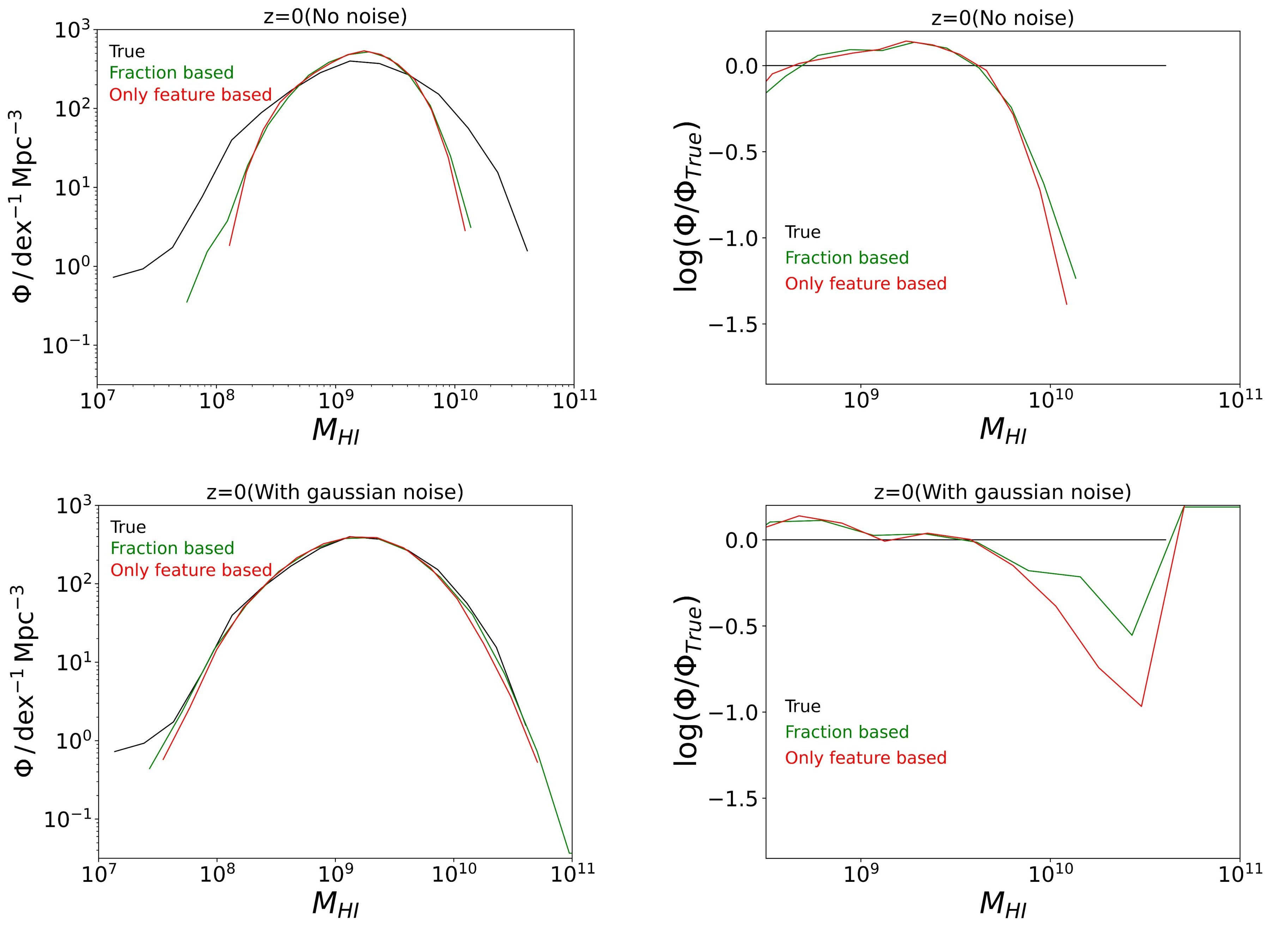
Figure 7: This figure shows mass functions of $M_{\rm HI}$ at $z=0$. The left column has the true, fraction-based, and feature-based mass functions and the right column has the same values divided by the true values. The upper row has the results from the ML prediction and the lower row has the ML predictions with the gaussian noise values.

5.2 Mass function predictions

Using our approach of including the ML scatter, we plotted the resulting mass functions from our ML framework for the only feature-based approach and the fraction-based approach (wherever computed) in Figure 8(a,b) (left column), along with the mass functions of the true values. The plots on the right column are the ratio plots related to their left plot, where all the mass functions are divided by the true mass function values for better visualization of the deviation. If, in some cases, we have ML predictions beyond the true spectrum, we shift the ML prediction values to the top boundary in the ratio plot. We also shift the lower boundary of the ratio plot to the lower limit of the feature where we add the scatter bias.

Using the postprocessing step that incorporates the ML scatter adjustment, we plot the resultant mass functions for the true, feature-based, and fraction-based approaches in Figure 8(a,b) left column. The right column in Figure 8(a,b) features ratio plots corresponding to each mass function. In these ratio plots, all the mass functions are normalized by the true mass function values, providing a clearer visualization of any discrepancies. For instances where the ML predictions exceed the range of the true spectrum, the ML prediction values are shifted to the upper boundary of the plot. On the other hand, the lower boundary of the ratio plot is adjusted to align with the threshold which has roughly 90% mass (SFR value) above it for the SF subgroup. Note that this boundary is just for better visualization and is not involved in any of the computations.

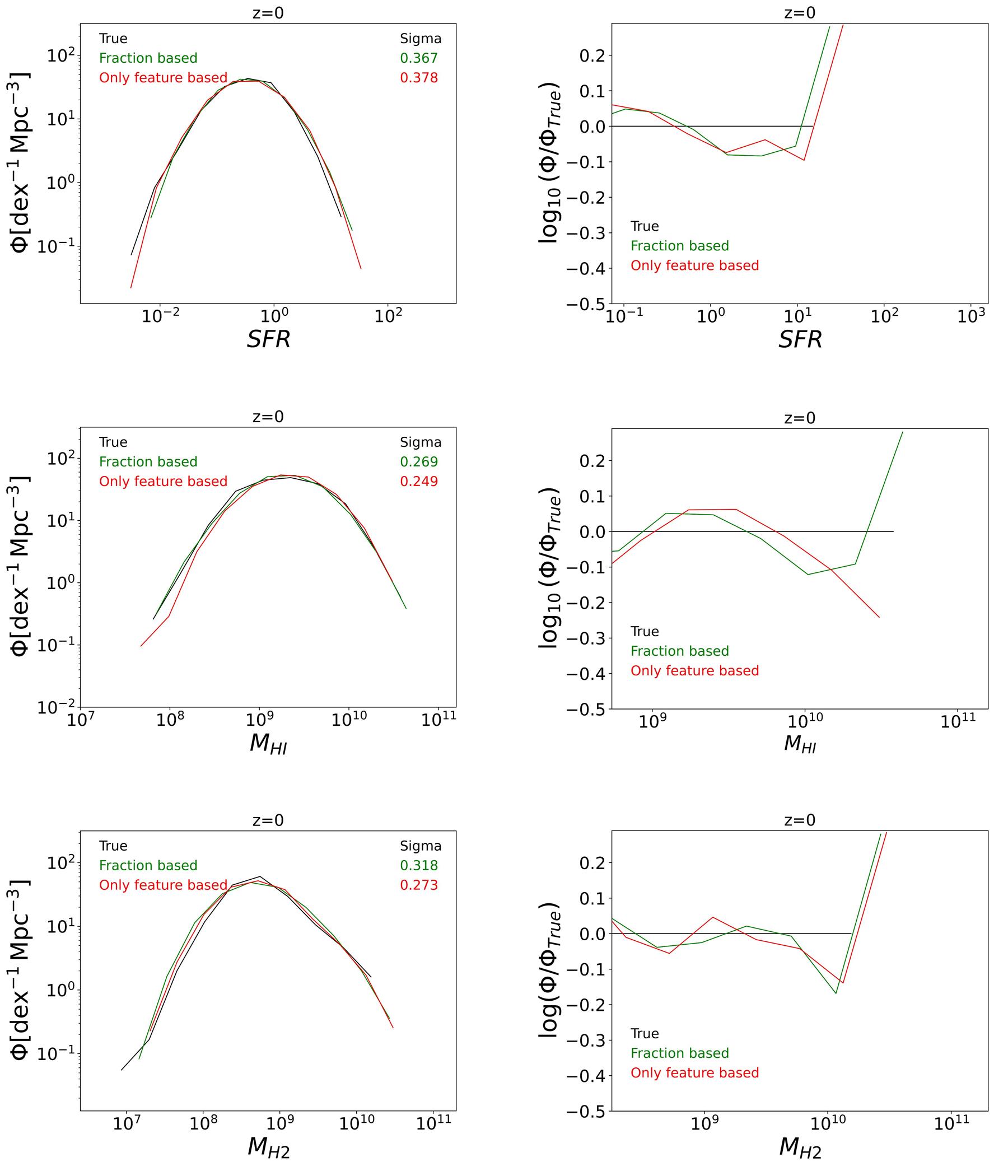
(a) Central galaxies

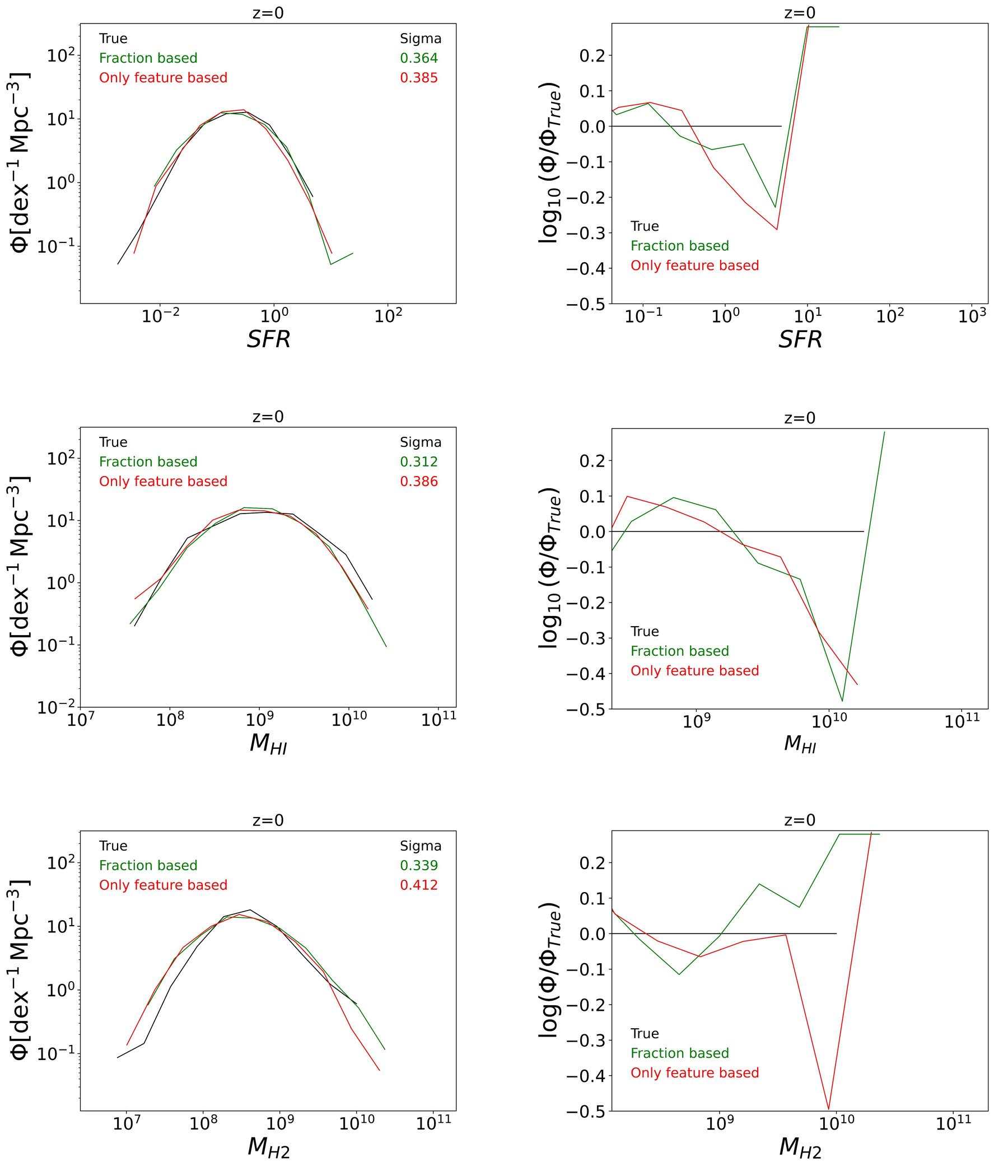
(b) Satellite galaxies

Figure 8: Mass function plots of true and predictions (with added ML scatter) from the best-performing frameworks for both fraction-based and feature-based approaches using Simba simulation at z=0. The left column has the exact mass functions. Also in these plots, each approach’s $\sigma$ value is mentioned on the top right corner in the same color code as the label. The right one has these values normalized with the mass function from the true value for a better comparison.

5.2.1 SFR

Following the methodology explained above, keeping the center of the gaussian at 0, we vary the standard deviation from 0.0 to 1.0 with an interval of 0.001 for both approaches. The noise for the SFR approach has a slightly higher standard deviation than the sSFR approach with a value of 0.378 compared to 0.367 and 0.385 compared to 0.364 for central and satellite galaxies respectively as shown in Figure 8(a,b) first row.

With the added noise central galaxy predictions came pretty close to the true spectrum and were roughly $\pm$ 0.1 around the true values. The predictions have some underprediction around the middle of the ratio plot with a shift to overprediction towards either edge. For satellite galaxies, the fraction-based approach stayed closer to the true values for most of the spectrum as shown in the ratio plot.

5.2.2 $M_{\rm HI}$

$M_{\rm HI}$ predictions are also processed in a similar way to SFR predictions. The noise for the $M_{\rm HI}$ approach has a slightly lower standard deviation than the $M_{\rm fHI}$ approach with a value of 0.249 compared to 0.269 as shown in Figure 8(a) second row. For satellite galaxies $M_{\rm HI}$ approach has a higher standard deviation at 0.386 compared to 0.312 for the $M_{\rm fHI}$ approach shown in Figure 8(b) second row.

For central galaxies, the addition of noise brought the fraction-based spectrum into $\pm$ 0.1 deviations from the true value. The only feature-based approach however can be seen performing slightly worse than this going to -0.2 values at higher mass. For satellite galaxies, both approaches are seen to be deviating from the true spectrum at higher mass values.

5.2.3 $M_{\rm H2}$

Our $M_{\rm H2}$ predictions are relatively more accurate than $M_{\rm HI}$ and SFR predictions. With the added scatter bias, this turned out better as shown in the ratio plots of Figure 8(a,b) third row. The noise for the $M_{\rm H2}$ approach has a lower standard deviation than the $M_{\rm fH2}$ approach with a value of 0.273 compared to 0.318 as shown in Figure 8(a) third row. For satellite galaxies $M_{\rm H2}$ approach has a higher standard deviation at 0.412 compared to 0.339 for the $M_{\rm fH2}$ approach shown in Figure 8(b) third row.

For central galaxies, the addition of noise brought the predicted spectrum into a pretty close  $\pm$ 0.05 deviations from the true value for most of the plot with a little more deviation towards the highest end. For satellite galaxies, both approaches are seen to be deviating from the true spectrum at higher mass values, but the over-prediction by the fraction-based is relatively less distant than the underprediction from the only feature-based approach.

6 Predictions at $z=1,2$

Until now, our exploration of the ML framework’s efficacy in predicting galaxy properties has been confined to $z=0$. However, to align our predictions with the broader scope of galaxy surveys or intensity mapping which often extend to higher redshifts, it is imperative to adapt and evaluate our ML models at $z=1$ and $z=2$, utilizing data from the Simba 100 Mpc box.

In this context, we have employed both fraction-based and feature-based approaches for predicting SFR, $M_{\rm HI}$, and $M_{\rm H2}$ at $z=1$ and $z=2$. As with the $z=0$ scenario, these predictions at higher redshifts commence with the application of a preclassifier, as illustrated in the classifier layer of Figure 1. This crucial step involves setting a boundary for sSFR, defined by Equation 2, which simplifies to $10^{-10.5}$${yr}^{-1}$ for $z=0$. Following this guideline, various models are trained by the procedure provided in subsection 3.4.

In the process of classifying galaxies, at both $z=1$ and $z=2$, the Voting method, which aggregates predictions from three ML models, yielded the highest NPV for both central and satellite galaxies as shown in Figure 9. For the central galaxies at both redshifts, a galaxy is classified Q by Voting if identified as such by either RF, the model from TPOT, or the model from AutoKeras. For satellite galaxies at $z=1$, Voting predicts Q when either RF, TPOT, or AutoKeras suggests this status, whereas at $z=2$, this determination is made when predictions from RF, AutoSklearn, or AutoKeras align with a Q classification.

The classifier has demonstrated decent efficiency in segregating Q from SF galaxies across both central and satellite populations at $z=1$. Specifically, central galaxies exhibit a NPV of 0.62, while satellites present a better NPV of 0.73. The reduction in $NPV$ from $z=0$ is simply because the Q fraction is much less compared to what we had for the lower redshift; 5.99% vs 17.35% for central and 25.77% vs 53.58% for satellite galaxies. Considering such a low fraction of Q galaxies, getting such an NPV is decent. At $z=2$, the values however are not so impressive. For central galaxies it is just 0.24 and for satellites, it’s slightly better at 0.56. These results come from an even lower Q fraction than $z=2$; just 1.55% for central galaxies and 11.25% for satellite galaxies.

At $z=1$ the classifier effectively segregates Q from SF galaxies for both centrals and satellites. Central galaxies achieve an NPV of 0.62, while satellites yield a slightly higher NPV of 0.73. The decrease in NPV from $z=0$ to $z=1$ reflects a diminished Q fraction; 17.35% versus 5.99% for centrals and 53.58% versus 25.77% for satellites. Considering the substantial reduction in the fraction of Q galaxies at higher redshifts, approximately halving for satellites and decreasing by a factor of three for centrals, the performance of the ML algorithms is commendable. At $z=2$, the fraction of Q galaxies diminishes further, accounting for only 1.55% of central galaxies and 11.25% of satellites. This significant reduction in the Q population results in less impressive NPV outcomes, with a value of 0.24 for central galaxies and a marginally better 0.56 for satellites. The sharp decrease in the presence of Q galaxies at this higher redshift challenges the predictive capability of the ML algorithms, as reflected in the decrease of NPV values, especially for central galaxies.

Moving ahead we implement the regressor models as outlined in subsection 3.5 in a similar way to $z=0$. In Figure 10, we present the optimal models derived from both our fraction-based and feature-based approaches at $z=1$, and $z=1$. The predictions from these models are then plotted against the true values in Figure 11(a, b) where a detailed comparison is made between the fraction-based and feature-only approaches for the prediction of concerned features at $z=1$ (top three rows) and $z=2$ (bottom three rows). In the following subsection, we give a detailed comparison of these with the accuracies of our models. We also present the mass functions for both approaches in a similar way to $z=0$, in Figure 12.

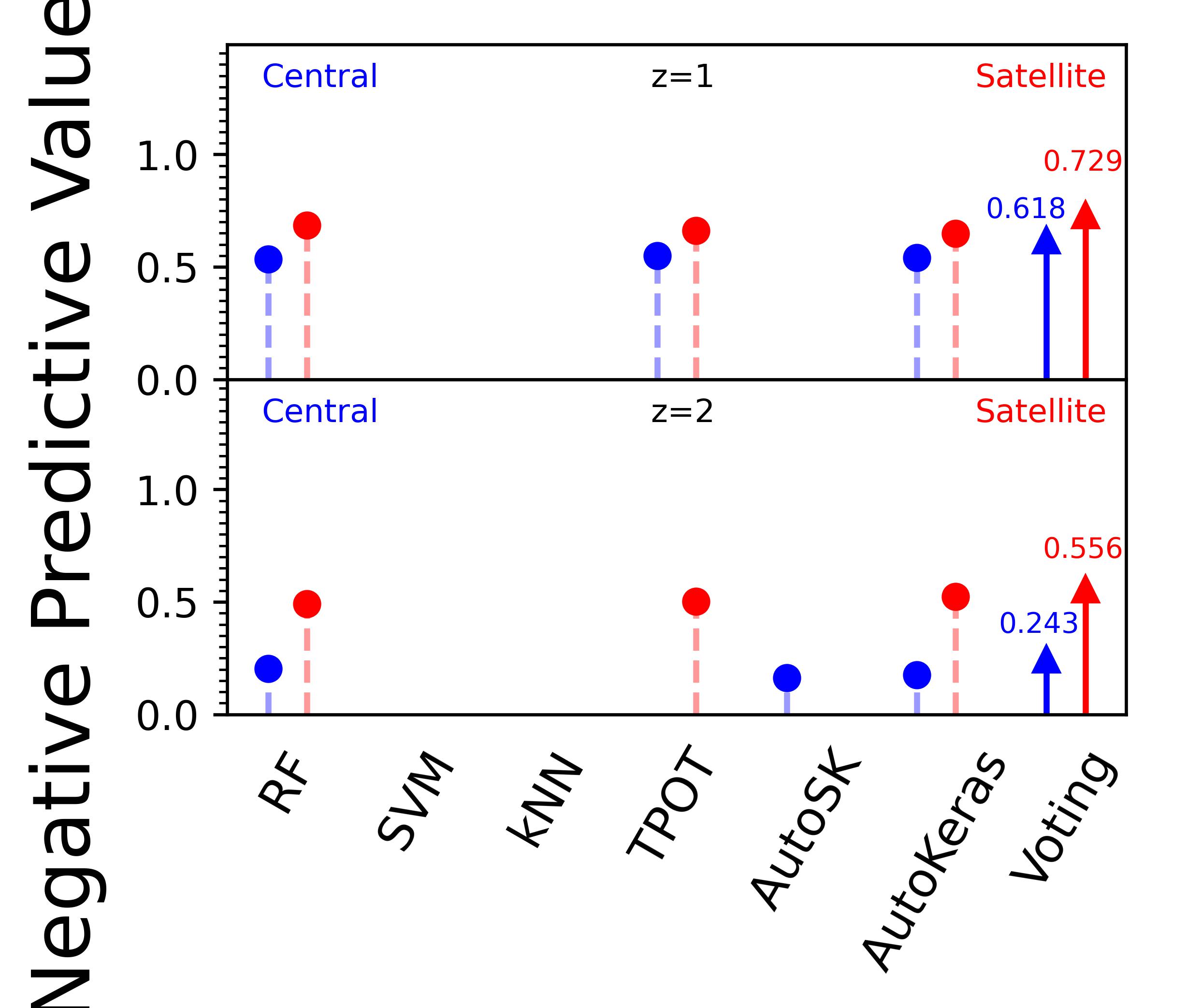
Figure 9: Classifier models

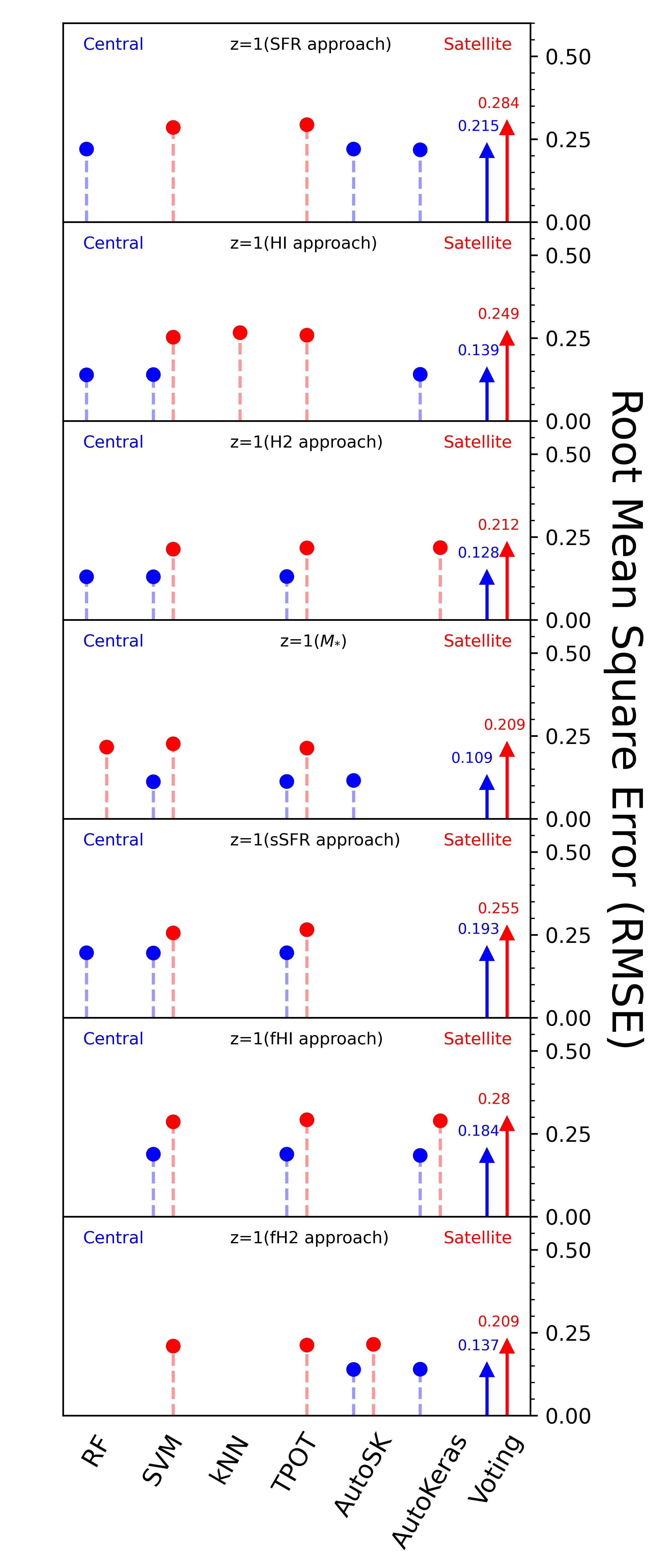
(a) z=1

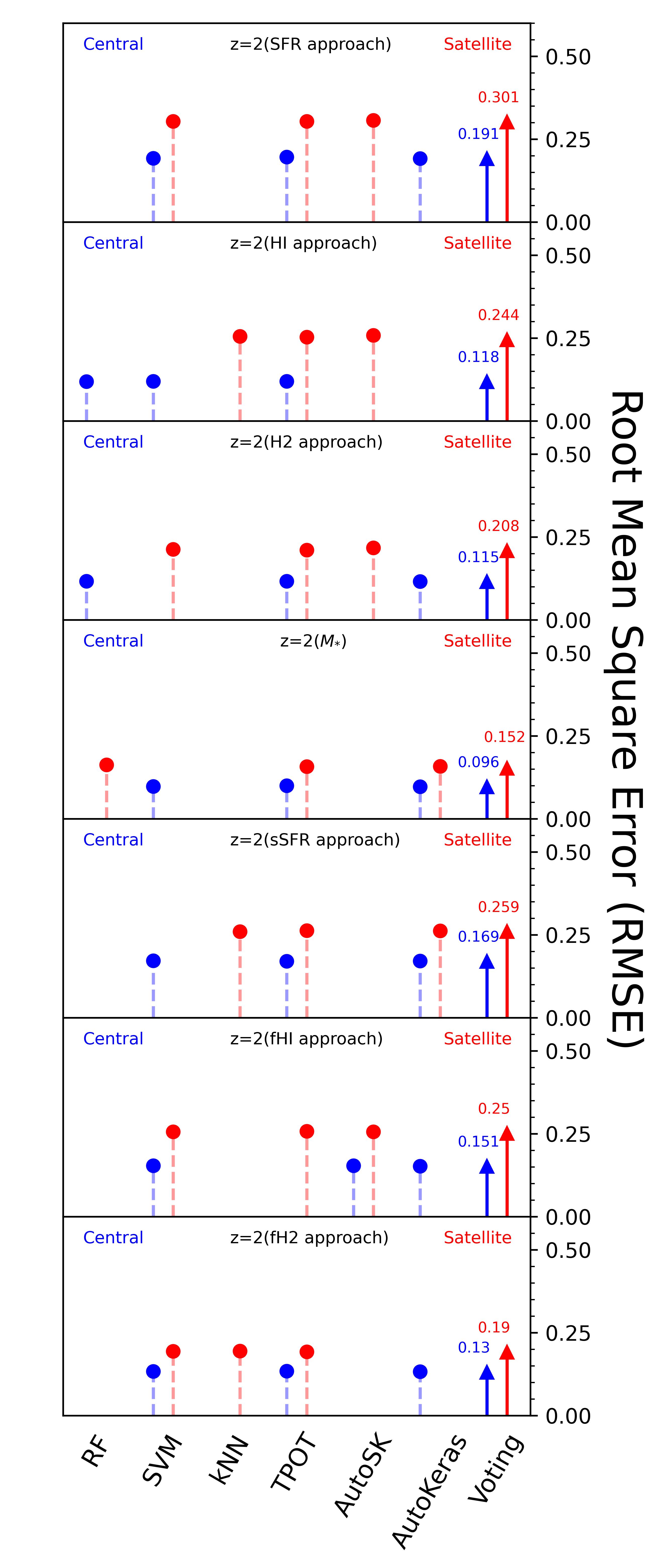
(b) z=2

Figure 10: Plot (a) has feature-wise comparison among classifier and (b) has comparison among regressor algorithms of both central (blue) and satellite (red) galaxies on the respective test datasets of Simba simulations at $z=1,2$. In (a) we plot the $NPV$ values from the classifier algorithms for the test data. The algorithm having the highest $NPV$ value for a feature is denoted by the triangle at the head with the corresponding $TNR$ value mentioned just above it. In (b) we show the $\sigma$ values from the regressor algorithms for the test data. The algorithm having the lowest $\sigma$ for a feature is denoted by the triangle at the head, with the corresponding $\sigma$ mentioned just above it. In both (a) and (b), if Voting is the best performing algorithm, the participating algorithms for Voting are also plotted with dotted lines and a circle on the top.

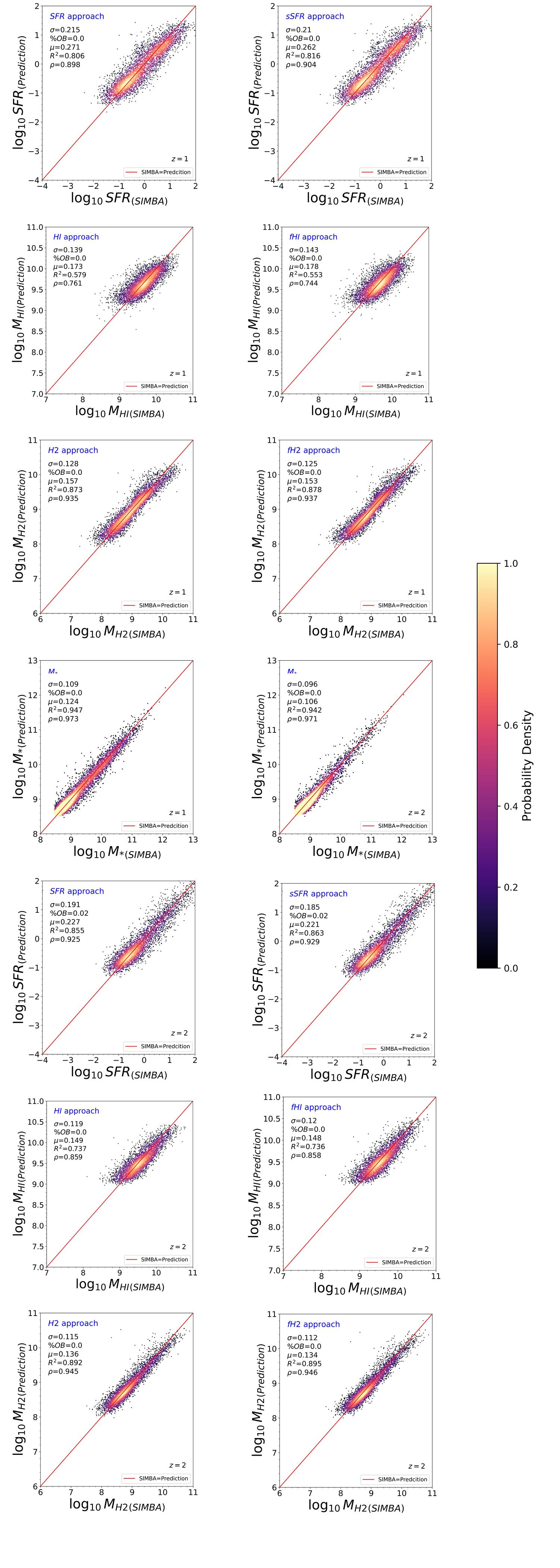
(a) Central Galaxies

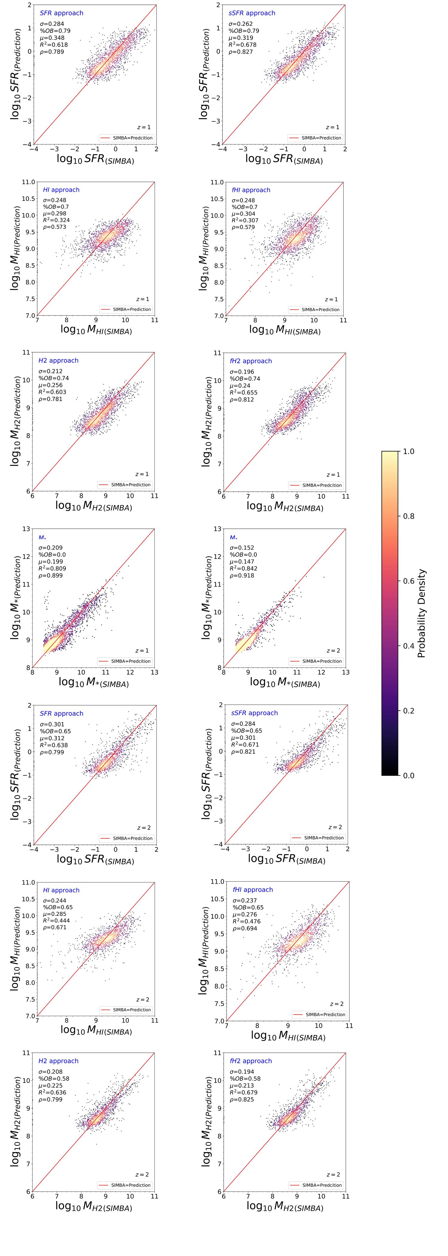
(b) Satellite Galaxies

Figure 11: The best-performing frameworks for both fractions-based and only feature-based approaches were implemented on the entire Simba simulation at z = 1 and 2 to predict SFR, $M_{\rm HI}$, and $M_{\rm H2}$. (a) has ML predictions for central galaxies and (b) has for satellite galaxies. The top three rows are at z=1 and the bottom three at z=2 in both (a) and (b)

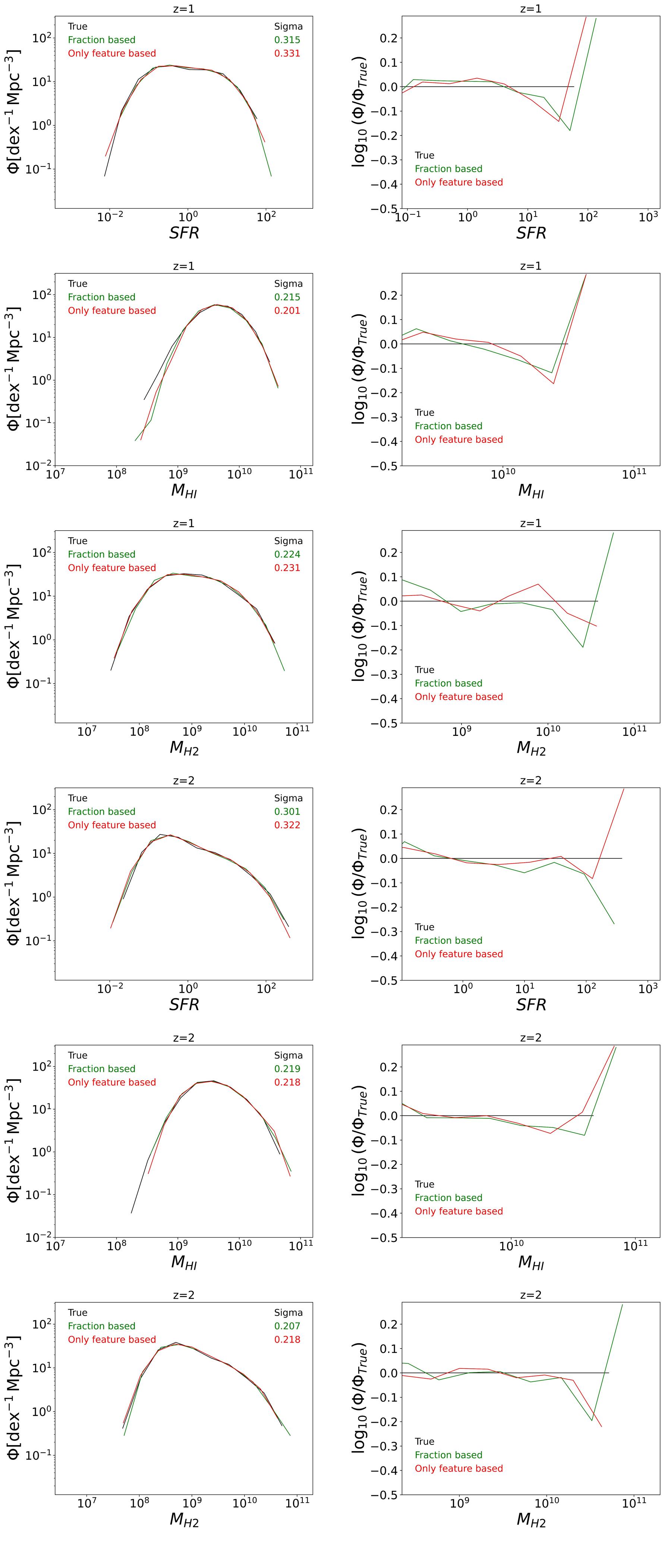
(a) Central galaxies

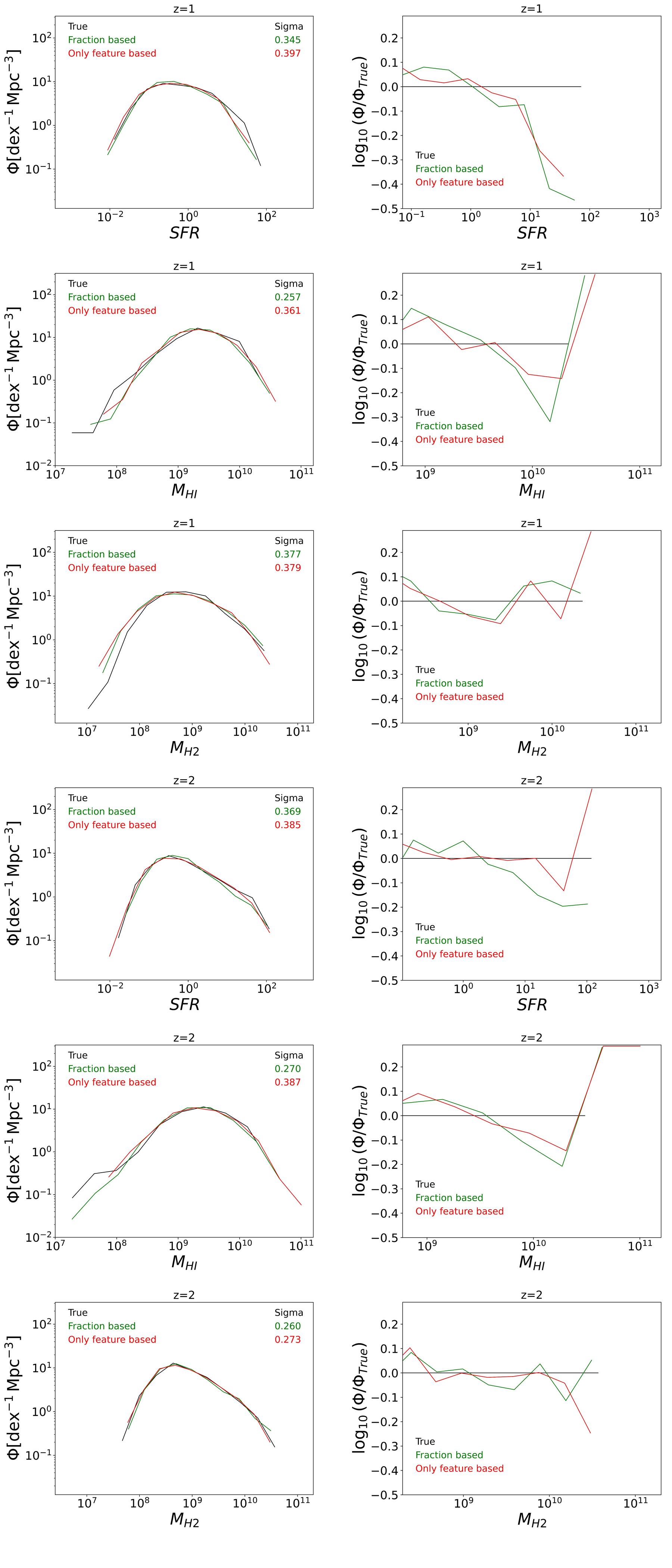
(b) Satellite galaxies

Figure 12: Mass function plots of results (with added ML scatter) from the best-performing frameworks for both fraction-based and feature-based approaches using Simba simulation at z=1 (a) and at z=2 (b). The left columns in both (a) and (b) have the exact mass functions. Also in these plots, each approach’s $\sigma$ value is mentioned on the top right corner in the same color code as the label. The right ones have these values divided with the mass function from the true value for a better comparison.

6.1 SFR

6.1.1 $z=1$

At $z=1$, Voting achieved the best RMSE for predicting both traditional and fractioned-based approaches for central galaxies. As illustrated in the first and fifth rows of Figure 10(a), for central galaxies, Voting combines predictions from RF, the model from AutoSklearn, and the model from AutoKeras for the SFR approach. Conversely, for the sSFR approach, the ensemble integrates results from RF, SVM, and the model from TPOT.

For satellite galaxies, Voting again has the best RMSE, across both approaches. In this case, Voting combines results from SVM and the model from TPOT. It is important to note that in many cases not all the algorithms we test the data on exhibit significant predictive accuracy. The choice to limit the Voting ensemble to these models is driven by the clear performance gap observed, with additional models from our selection not achieving comparable levels of accuracy. Consequently, the addition of any other algorithms into our Voting strategy for satellite galaxies was deemed counterproductive, reducing the ensemble’s overall precision. Thus, a deliberate selection of only two (not three) of the most effective algorithms for the Voting process was made to avoid the addition of other much less accurate algorithms.

Implementations of these algorithms are shown in Figure 11(a,b) first row. For central galaxies, both of our approaches have similar statistical outcomes with the fraction-based approach demonstrating a marginal advantage. The sSFR approach achieves a $\sigma$ of 0.21 compared to 0.22 from the SFR approach and a $R^{2}$ of 0.82 over 0.81. However, for satellite galaxies, as illustrated in Figure 11(b) first row, the predictions state a clear superiority of the fraction-based approach over the traditional method. The fraction-based approach elevated $R^{2}$ from 0.62 to 0.68 and the Pearson correlation coefficient from 0.79 to 0.83. Visually, this method also presents a reduction in the number of outliers, especially at higher SFR values, indicating a more accurate and reliable prediction model for satellite galaxies.

In the post-processing phase, similar to the procedures for $z=0$, we add random Gaussian scatter to both central and satellite galaxies for both the approaches. For central galaxies, SFR approach has a slightly more standard deviation at 0.331 than 0.315 for the sSFR approach as shown in Figure 12(a) first row. The ratio plots here look remarkable accuracy, with very low deviation till high SFR values, particularly for the fraction based approach with $\pm$  0.05 deviation from the true value.

For satellite galaxies, the SFR approach also manifests a higher standard deviation at 0.397 compared to 0.345 for the sSFR approach, as shown in Figure 12(b) first row. Both approaches showed decent results, with deviations up to $\pm$ 0.1 from the true values till the upper half of the ratio plot, followed by under-predictions.

6.1.2 $z=2$

Here Voting achieved the best RMSE for predicting both traditional and fractioned-based approaches for central galaxies. As illustrated in the first and fifth rows of Figure 10(b), for central galaxies, Voting combines predictions from SVM, the model from TPOT, and the model from AutoKeras for both SFR and sSFR approach.

For satellite galaxies, Voting again has the best RMSE, across both approaches. In this case, Voting combines results from SVM, the model from TPOT and the model from AutoSklearn for the SFR approach and kNN, the model from TPOT, the model from AutoKeras for the sSFR approach.

The implementations of these algorithms are demonstrated in the fifth row of Figure 11(a, b). For central galaxies, the fraction-based approach demonstrates a marginal yet notable improvement over the traditional method. This enhancement is quantified by achieving a $\sigma$ of 0.185 compared to 0.191 and an $R^{2}$ of 0.863 compared to 0.855. For satellite galaxies, the improvements of the fraction-based approach become more pronounced, as depicted in the fifth row of Figure 11(b). Here, the fraction-based method raised $R^{2}$ from 0.64 to 0.67 and reduced $\sigma$ from 0.3 to 0.28.

Following this, random Gaussian scatter is added to both central and satellite galaxies for both approaches. For central galaxies, the SFR approach resulted in a standard deviation of 0.322, slightly higher than the 0.301 for the sSFR approach, as shown in Figure 12(a) fourth row. The ratio plots here display impressive accuracy at $z=1$, with a very low deviation of $\pm$  0.05 deviation from the true value up to high SFR values.

For satellite galaxies, the SFR approach exhibited a higher standard deviation of 0.385, compared to 0.369 for the sSFR approach, as depicted in the fourth row of Figure 12(b). Both methodologies yield respectable outcomes, with deviations maintained at $\pm$ 0.1 from the true values up to the midpoint of the ratio plot, followed by under-predictions.

For satellite galaxies, the SFR approach also shows a higher standard deviation at 0.385 compared to 0.369 for the sSFR approach, as shown in Figure 12(b) fourth row. Both approaches showed decent results, with deviations confined to $\pm$ 0.1 from the true values till the upper half of the ratio plot, followed by under-predictions.

6.2 $M_{\rm HI}$

6.2.1 $z=1$

For $M_{\rm HI}$ predictions at $z=1$, Voting achieved the best RMSE for predicting both traditional and fractioned-based approaches for central galaxies. As illustrated in the second and sixth rows of Figure 10(a), for central galaxies, Voting combines predictions from RF, SVM, and the model from AutoKeras for the HI approach. For the fHI approach, the ensemble integrates results from SVM, the model from TPOT, and the model from AutoKeras.

Similarly, for satellite galaxies, Voting also secures the best RMSE across both approaches. In this case, Voting combines results from SVM, kNN, and the model from TPOT for the HI approach and SVM, the model from TPOT and the model from AutoKeras.

The implementations of these algorithms, as showcased in the second row of Figure 11(a, b), reveal that for central galaxies, both approaches yield comparable statistical performances. The HI approach however has a slight edge with a $\sigma$ of 0.139 against 0.143 from the fHI approach. For satellite galaxies, as illustrated in Figure 11(b) second row, the predictions for both approaches are nearly identical, registering a $\sigma$ of 0.25. The fraction-based approach has a bit more outliers, but unlike the underprediction at higher mass for the traditional approach, it has a symmetric prediction.

Similar to the post-processing for SFR predictions, we add random Gaussian scatter to both central and satellite galaxies for both the approaches. For central galaxies, fHI approach has a slightly more standard deviation at 0.215 than 0.201 for the HI approach as shown in Figure 12(a) second row. The ratio plots here have low deviation till high $M_{\rm HI}$ values with $\pm$  0.1 deviation from the true value.

For satellite galaxies, the HI approach has much higher standard deviation at 0.361 compared to 0.257 for the fHI approach, as shown in Figure 12(b) second row. Both approaches showed decent results for the central $M_{\rm HI}$ values, with over and under prediction before and after that.

6.2.2 $z=2$

At $z=2$ Voting achieved the best RMSE for predicting both traditional and fractioned-based approaches for central galaxies. As illustrated in the second and sixth rows of Figure 10(b), for central galaxies, Voting combines predictions from RF, SVM, and the model from TPOT for the HI approach and fHI approach ensembles SVM, the model from AutoSklearn, and the model from AutoKeras.

For satellite galaxies, Voting again has the best RMSE, across both approaches. In this case, Voting combines results from SVM, the model from TPOT and the model from AutoSklearn for the HI approach and kNN, the model from TPOT, the model from AutoSklearn for the fHI approach.

The implementations of these algorithms are visually represented in the sixth row of Figure 11(a, b). For central galaxies, both approaches show the same statistics; $\sigma$ from 0.12, $R^{2}$ of 0.74, and a perason coefficient of 0.86. For satellite galaxies, the improvements of the fraction-based approach is more visible, as depicted in the sixth row of Figure 11(b). Here, the fraction-based method raised $R^{2}$ from 0.44 to 0.48 and Pearson coefficient from 0.67 to 0.69. Visually the results also get more symmetric around the 1:1 trend for the fraction-based approach.

Finally, on the post-processing step, similar to $z=1$, we add random Gaussian scatter to both central and satellite galaxies for both the approaches. For central galaxies, both the approaches have almost equal standard deviation of 0.218 and 0.219 for HI and fHI approach respectively as shown in Figure 12(a) fifth row. The ratio plots here remarkably low deviation till high $M_{\rm HI}$ values with $\pm$  0.1 deviation from the true value.

For satellite galaxies, the HI approach has much higher standard deviation at 0.387 compared to 0.270 for the fHI approach, as shown in Figure 12(b) fifth row. Both approaches showed decent results at the central $M_{\rm HI}$ values, with slight over and under prediction before and after that.

6.3 $M_{\rm H2}$

6.3.1 $z=1$

For $M_{\rm H2}$ predictions at $z=1$, the Voting method delivered the best RMSE for both traditional and fraction-based approaches for central galaxies, as depicted in the third and seventh rows of Figure 10(a). For the H2 approach, Voting aggregates predictions from RF, SVM, and the model from TPOT. The fraction-based approach, conversely, employs a combination of models from AutoSklearn and AutoKeras. Notably, here we have two algorithms for Voting similarly as for the SFR predictions at $z=1$, as explained in subsubsection 6.1.1.

For satellite galaxies, Voting consistently achieves the optimal RMSE for both the H2 and fH2 approaches. This ensemble for the H2 approach integrates results from SVM, the model from TPOT, and the model from AutoKeras, while for the fH2 approach, it incorporates predictions from SVM, the model from TPOT, and the model from AutoSklearn.

The performance of these algorithms, showcased in the third row of Figure 11(a, b), indicates comparable statistical outcomes for central galaxies across both approaches. However, the fH2 approach slightly outperforms the traditional approach, achieving a $R^{2}$ of 0.88 compared to 0.87. Visually, predictions around the central mass values for the fH2 approach appear significantly tighter than those for the H2 approach. For satellite galaxies, as presented in Figure 11(b) second row, the fraction-based approach notably surpasses the traditional method, with a $R^{2}$ of 0.66 against 0.6, a Pearson coefficient of 0.81 versus 0.78, and a $\sigma$ of 0.2 compared to 0.21. Visually, the predictions from the fraction-based approach are closer to the true values.

Similar to the post-processing for $M_{\rm HI}$ predictions, we add random Gaussian scatter to both central and satellite galaxies for both approaches. For central galaxies, the fH2 approach has a higher standard deviation at 0.318 than 0.273 for the H2 approach, as shown in Figure 12(a) third row. The ratio plots here have low deviation till high $M_{\rm H2}$ values with $\pm$  0.1 deviation from the true value.

For satellite galaxies, both approaches have almost equal standard deviations of 0.379 and 0.377 for the H2 and fH2 approaches respectively, as shown in Figure 12(b) third row. Both approaches also show decent results for the satellite values, with $\pm$  0.1 deviations from the true value.

6.3.2 $z=2$

At $z=2$, the Voting method once again performs best, achieving the lowest RMSE in both traditional and fraction-based approaches for central galaxies. This optimal performance is delineated in the third and seventh rows of Figure 10(b), where, for the H2 approach, Voting combines predictions from RF, the model from TPOT, and the model from AutoKeras. For the fraction-based approach, the ensemble leverages SVM, the model from TPOT, and the model from AutoKeras.

Similarly, for satellite galaxies, Voting continues to deliver the best RMSE for both prediction approaches. Here, the H2 approach utilizes SVM, the model from TPOT, and the model from AutoSklearn, while the fH2 approach integrates SVM, kNN, and the model from TPOT.

Visual representations of these algorithmic implementations, as shown in the seventh row of Figure 11(a, b), reveal that for central galaxies, both approaches produce similar statistical outcomes. Nevertheless, the fH2 approach marginally surpasses the traditional method, achieving a $R^{2}$ of 0.9 compared to 0.89. For satellite galaxies, as evidenced in Figure 11(b) seventh row, the fraction-based approach significantly outperforms the traditional approach, with a $R^{2}$ of 0.68 against 0.64, a Pearson coefficient of 0.83 versus 0.8, and a $\sigma$ of 0.19 compared to 0.21. Visually, predictions from the fraction-based approach align more closely with true values, exhibiting fewer outliers.

In the final post-processing step, similar to $z=1$, we add random Gaussian scatter to both central and satellite galaxies for both approaches. For central galaxies, both the approaches have almost equal standard deviations of 0.231 and 0.224 for the H2 and fH2 approaches respectively as shown in Figure 12(a) sixth row. The ratio plots here remarkably low deviation till high $M_{\rm HI}$ values with  0.2 deviations from the true value near the higher end of the spectrum.

For satellite galaxies, the H2 approach has a higher standard deviation at 0.273 compared to 0.260 for the fH2 approach, as shown in Figure 12(b) sixth row. Both approaches showed low deivitaion of $pm$  0.1 throughout the spectrum except for H2 getting a larger udnerpredcition at the highest end.

Overall, for quantities at higher redshifts, we see generally improved prediction in the regressors, indicating that more accurate predictions are available at earlier epochs. As at $z=0$, the fraction-based approach slightly outperforms the feature-based approach.

7 Feature importance from Random Forest

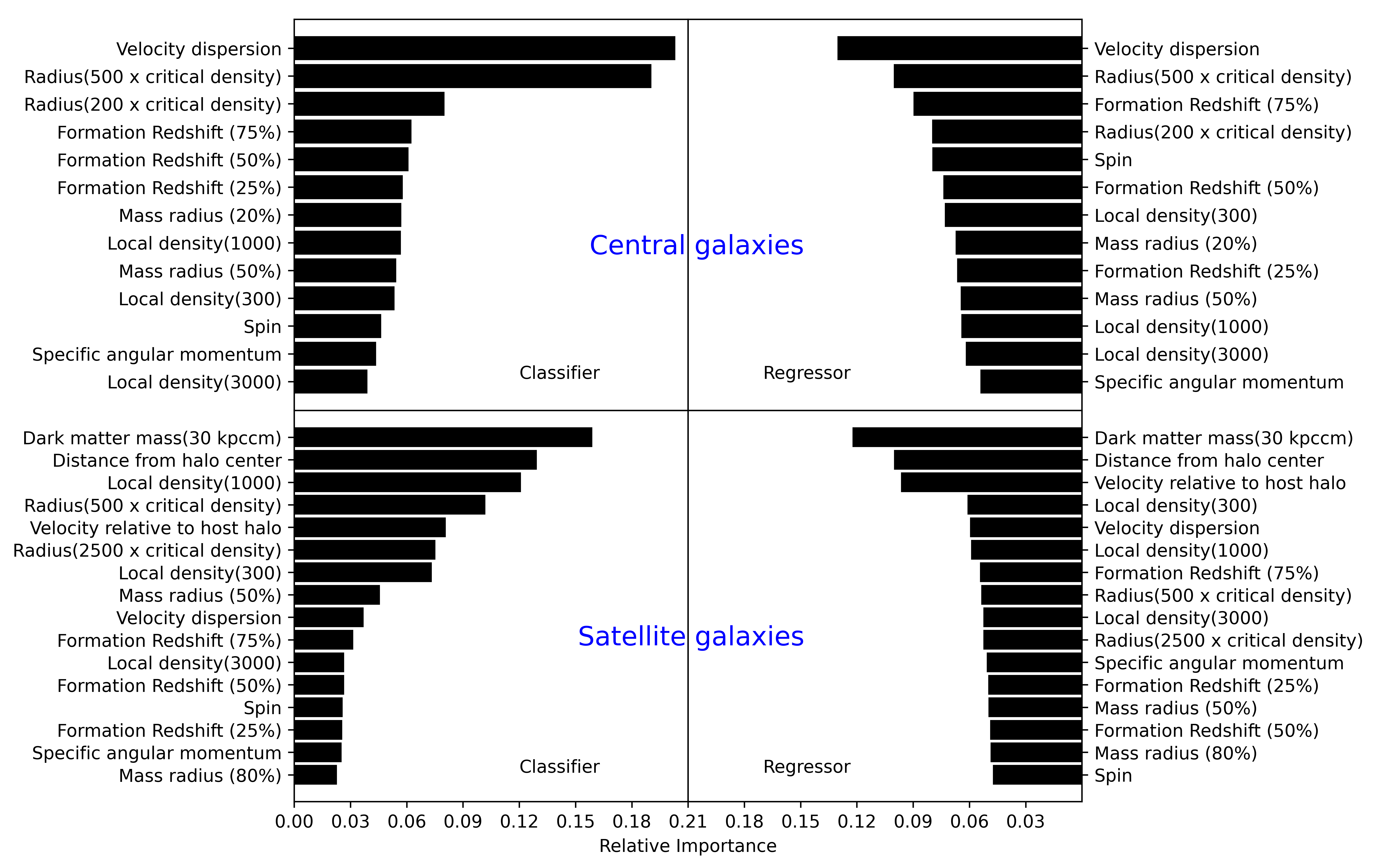
Figure 13: This figure shows the feature importance as derived by the Random Forest (RF) algorithm. The upper row has the results for the central galaxies and the lower one is for satellite galaxies. The left column represents a classifier feature importance and the right one to a regressor. The length of each bar corresponds to the relative importance of a specific halo property by the RF algorithm to infer the $M_{\rm HI}$ content in galaxies using the only feature-based approach.

It is interesting to examine which input features are driving the predictions, in order to gain some insights into the physics that the ML is learning. To determine the feature importance for our input features at $z=0$, we use the Random Forest algorithm available in the Scikit-Learn library. Unfortunately, feature importance is only available using this ML method, so we cannot examine it for our full pipeline, but nonetheless it may yield some interesting insights. To provide a clear visual representation, Figure 13 selectively presents the feature importance only for the sSFR predictions.

In the analysis of central galaxies, velocity dispersion emerges as the most significant feature for both classifier and regressor models. This aligns with previous findings, where velocity dispersion was shown to strongly correlate with sSFR, suggesting a deep interconnection between the kinematics of a galaxy and its star-forming activity (Pelliccia et al., 2020; Yu et al., 2019). Next in the line are the radius measurements at various multiples of the critical density. These radii measurements are tied to the galaxy’s spatial and mass distribution, affecting its gravitational potential and star formation rates.

For satellite galaxies, features such as dark matter mass within a 30 kpc radius, velocity relative to the host halo, and distance from the halo center turned out to be quite important. Features like these could be directly linked to processes such as ram-pressure stripping, tidal interactions, and halo-related quenching mechanisms  (Yoon et al., 2017; Smith et al., 2016).

8 Comparison with other works

A similar framework to us on MUFASA (Davé et al., 2016) simulation was done by Agarwal et al. (2018). However, their work is limited to central and star-forming galaxies, unlike this paper. Another work on a combined training set of the EAGLE (Schaye et al., 2015) simulation plus the C-EAGLE (Barnes et al., 2017) cluster zoom simulations as done by Lovell et al. (2022). In this work, they highlighted the significant implications of halo-baryon ML models in larger periodic volumes. de Santi et al. (2022) used IllustrisTNG300 (Pillepich et al., 2018), and designed models for both central and satellite galaxies. Collectively, these studies have furnished ML frameworks capable of predicting various baryonic components within the host halo. However, automating the replication of entire N-body simulations has remained elusive. The primary reasons were limitations of their models in handling features of Q galaxies, and, in many cases, accounting for satellite galaxies as well. Our work aims to address these gaps by refining ML applications that can effectively interact with both SF and Q galaxies across the entire simulation spectrum.

9 SUMMARY

In this work, our primary goal is to enable ML models to predict the baryonic properties of halos from an entire N-body simulation, irrespective of the location or nature of the galaxy. The limitations of previous works in this area were in incorporating the subgroups involving satellite and quenched galaxies. Using the Caesar catalogues, we separate galaxies into centrals and satellites, then build regressor models for both subgroups to predict baryonic contents within them. To add the quenched galaxies to our framework, we pass the data through a pre-classifier. Then we train a regressor on the SF component of the classified data. The final accuracy depends on the results from both layers of ML algorithms. The ML frameworks show good accuracy even for fluctuating properties that have previously been more difficult to predict from halo properties alone, such as the SFR, H i mass, and H₂ mass. The frameworks show improved results for higher redshifts (Figure 11) since Simba has fewer quenched galaxies for $z=1,2$ than at $z=0$. A decrease in the number of quenched galaxies decreases the error in predictions from the classifier, which in turn enhances the performance of the regressor.

An interesting result was that, in most cases, the ML frameworks yielded somewhat better predictions when predicting the fraction relative to $M_{*}$, and then multiplying by the predicted $M_{*}$ value (see Figure 6 and Figure 11). This is somewhat counter-intuitive since it involves predicting two quantities separately and then multiplying them. but it turns out that the ML predicts $M_{*}$ quite accurately, so this does not hinder the overall predictive power. In the meantime, by dividing by $M_{*}$, the properties remove the “bigger is bigger” effect in the quantities, allowing the ML to focus on more subtle differences. At $z=O$, the fraction-based approach clearly showed better results for almost all the predictions, particularly in terms of not introducing a mass-dependent bias, while at $z=1,2$, it was less clear but the overall predictions were better. Hence the fractions-based approach seems to be the preferred alternative to optimize the accuracy.

The main difference between central and satellite galaxies within our study is the ratio of SF to quenched galaxies in these groups. At $z=0$, approximately 40% of satellite galaxies are quenched, in contrast to about 10% for central galaxies. This difference significantly influences the accuracy of our classifier predictions. Notably, in the satellite group, a larger fraction of quenched galaxies are misclassified as SF compared to the central group, primarily due to the higher prevalence of quenched galaxies in the satellite’s training set. Consequently, the SF galaxies used to train the regressor also include a higher proportion of quenched galaxies due to classification errors, particularly within the satellite group.

This discrepancy leads the ML algorithm to encounter a considerable number of quenched galaxies, prompting it to lower the output values for each feature in an attempt to optimize performance across the entire training dataset, encompassing both quenched and SF galaxies. As a result, this typically leads to under-predicted galaxy features, with more pronounced under-predictions for satellite galaxies than for centrals.

Addressing this issue could involve developing more robust classifiers specifically for satellite galaxies. Our results are generated from tests with several popular ML algorithms and their ensembles, along with both manual and automatic methods for optimizing their parameters. While further enhancement could be achieved through a more costly process involving an ensemble of sophisticated ML algorithms with finely tuned parameters (evaluating more significant digits), our current study establishes a benchmark for future research. As first in analyzing both satellite and quenched galaxies, we provide a benchmark for subsequent studies aiming to employ fully automated ML models across entire simulations to generate intensity maps, rather than focusing solely on subgroups.

A critical component of our methodology is the accurate recovery of the mass function, a key metric for intensity mappings. ML models typically train more effectively on high-density mid range values but tend to treat both the low and high ends of the distribution as outliers. This often results in a narrowing of the predicted mass function. To address this issue, we have implemented a novel post-processing correction to add a “ML scatter bias”. This method involves the addition of Gaussian noise to the mass function, specifically aimed at enhancing the representation of the high-mass end of the mass function, which plays a significant role in contributing to the intensity map.

Beyond these broad results, some more detailed key findings can be summarized as follows:

• Among the input features selected from Simba, velocity dispersion emerged as a key parameter in modeling central galaxies, followed by measurements of radii at various critical densities. For satellite galaxies, additional features such as dark matter mass and relative velocity and position to the host halo proved to be quite influential.

• The Voting method improved accuracy across all predictions and redshifts, as shown in Figure 4, Figure 5, Figure 9, and Figure 10. Notably, in a few cases, two ML algorithms significantly outperformed others, resulting in only two variables in the Voting ensemble compared to three for others.

• At $z=0$, the fraction-based approach greatly improved results for satellite galaxies and showed considerable improvement for central galaxies over the traditional approach. However, for H i predictions, the results were comparable to those of the traditional approach.

• At higher redshifts, our predictions were generally quite accurate, mainly because of the increase in the ratio of SF to Q galaxies, which reduced the number of outliers in the training set.

• Mass functions turned out to be quite helpful in demonstrating the advantages of the fraction-based approach. With a lower $\sigma$, the fraction-based approach achieved similar or better results than the traditional method, which required a higher $\sigma$ scatter bias in general. This was consistent across all cases involving satellite galaxies at different redshifts, though there were some exceptions for central galaxies.

A principal application of our ML framework is to simulate H i intensity maps. Our frameworks can simulate H i intensity maps tailored for upcoming astronomical surveys such as Hydrogen Intensity and Real-time Analysis eXperiment (HIRAX) (Newburgh et al., 2016) and the Square Kilometre Array (SKA) (Bacon et al., 2020). This can be done by applying our framework to very large-scale N-body simulations with sufficient volume to obtain a cosmologically representative sample of large-scale structure, while retaining enough resolution to properly resolve the lower-mass halos that dominate the H i content.

We further aim to improve the ML predictions for other galaxy quantities, such as emission line surveys that track the star formation rate and CO intensity mapping surveys that track the molecular hydrogen mass. Better and more sophisticated ways are required for the classifiers to improve the overall accuracy, in the process of automating ML models for the entire simulation. With a framework that can handle both centrals and satellites, and reliably isolate the star-forming gas-rich population, many applications open up for making predictions to future cosmology surveys in order to constrain both dark energy and the physical processes of galaxy evolution.

Data Availability

The article’s data will be shared on reasonable request to the corresponding author. The Simba simulation (Davé et al., 2019) data used in this article is available at http://simba.roe.ac.uk/.

Appendix A Generating Scatter plots

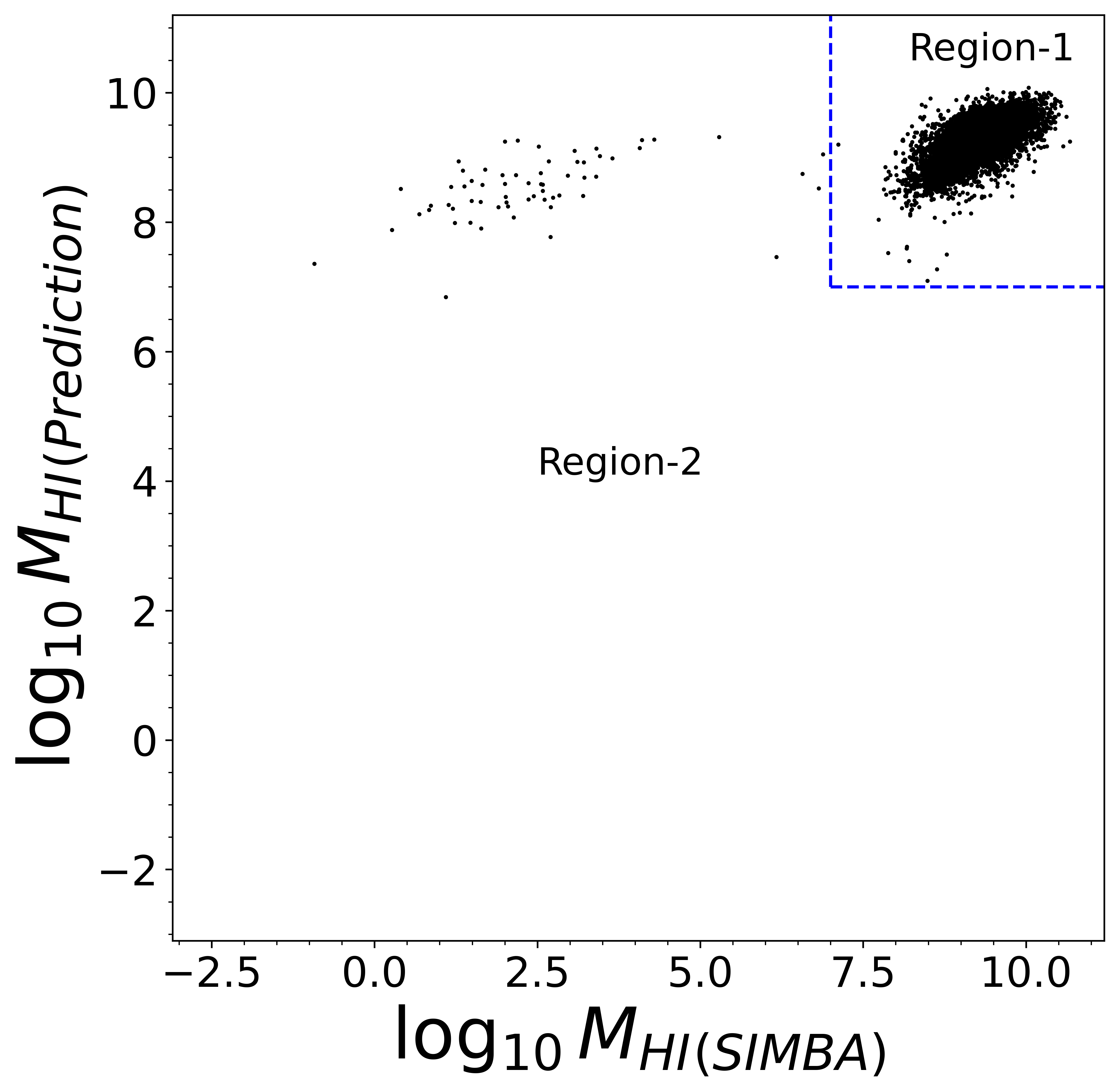
(a)

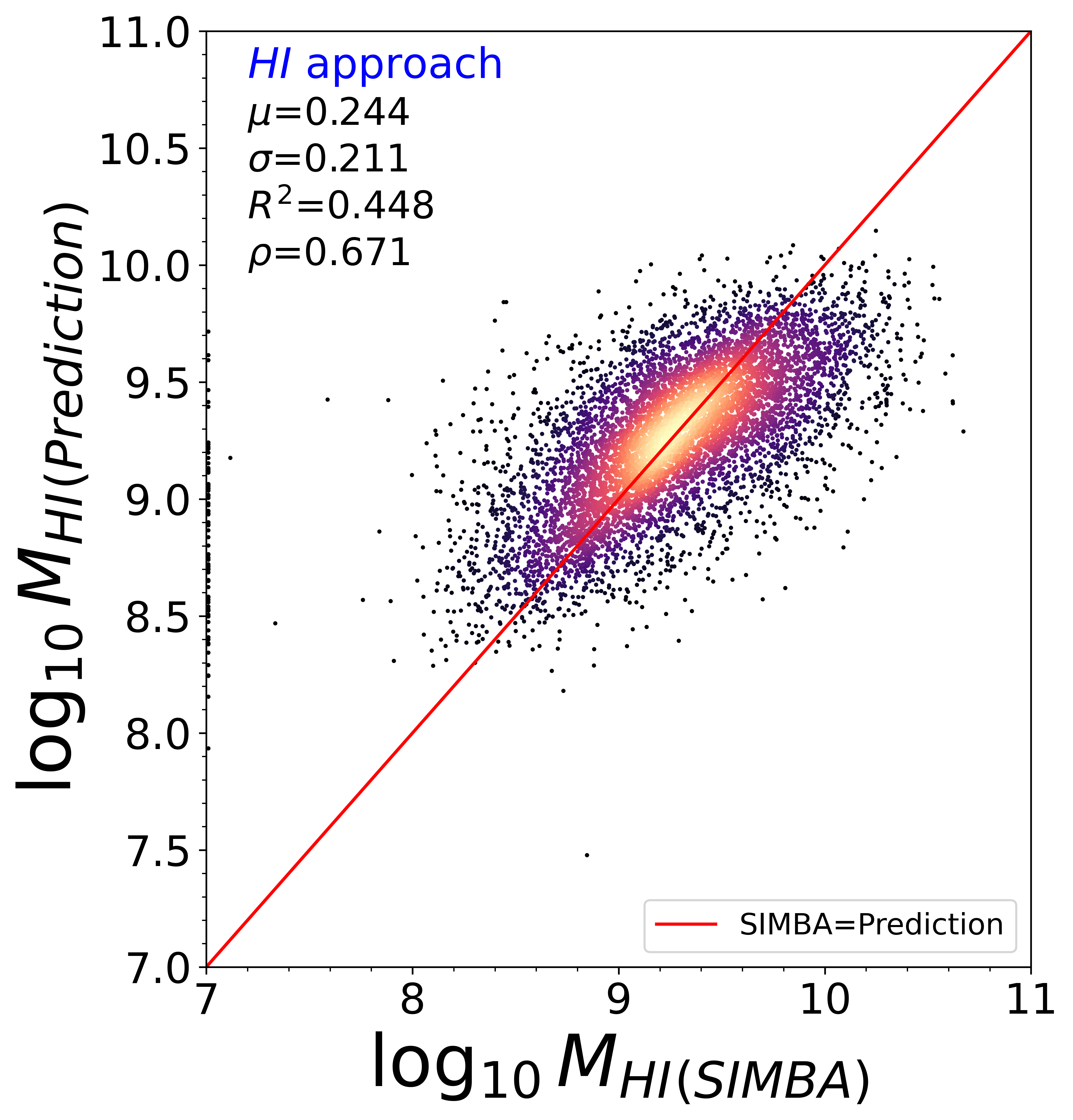
(b)

Figure 14: Here we show the process of making the scatter plots from the predicted data in our paper. Here we have taken the example of the HI approach at $z=0$, to generate the plots. (a) has final ML predictions using the HI approach at $z=0$ on the test data plotted against the true (Simba) values. The entire graph is divided into two groups (Region-1, and Region-2), through dotted blue lines. The lines are drawn at the quenched-Star forming boundaries. Region-1 has the SF data points from Simba, which got predicted as SF. Region-2 has SF data points from Simba, which got predicted as Q. (b) is the final plot that we use in our paper, which has the data points in region-1. Along with those, it also has the data points of the neighboring regions shifted to the nearest point on its boundary. The plots also have information about the plots along with a density-plot-like representation, to better visualize the distribution.

Figure 14 illustrates the process of making these scatter plots, for the sample of $M_{\rm HI}$, although the others work similarly. The full distribution of all galaxies is shown in panel (a). This is divided into four regions. Region 1 is where both Simba and the ML indicated substantial H i. Region 2 are galaxies that are actually Q in Simba but are predicted as SF by the ML. Region 3 has galaxies predicted as quenched by both (where the ML prediction for Q-classified galaxies is arbitrarily shown at 0), and Region 4 shows galaxies that are actually SF but are predicted as Q.

From the entire Simba simulation at $z=0$, Region 1 of the panel (a) has around 99.9% of the global $M_{\rm HI}$. So these misclassifications do not impact the overall H i budget hardly at all. This illustrates why we will primarily be concerned with Region 1, which is shown by itself in panel (b), with a 1:1 line shown in red. Since the points get saturated, we instead make a heat map of probability density, shown in panel (c). We further show all our computed metrics in the upper left. In the forthcoming sections, we will assess ML performance using figures as shown in panel (c) for all quantities and redshifts.

References

- Agarwal et al. (2018) Agarwal S., Davé R., Bassett B. A., 2018, Monthly Notices of the Royal Astronomical Society, 478, 3410
- Andrianomena et al. (2020) Andrianomena S., Rafieferantsoa M., Davé R., 2020, Monthly Notices of the Royal Astronomical Society, 492, 5743
- Bacon et al. (2020) Bacon D. J., et al., 2020, Publications of the Astronomical Society of Australia, 37, e007
- Barnes et al. (2017) Barnes D. J., et al., 2017, Monthly Notices of the Royal Astronomical Society, 471, 1088
- Benson (2012) Benson A. J., 2012, New Astronomy, 17, 175
- Bullock et al. (2001) Bullock J. S., Dekel A., Kolatt T. S., Kravtsov A. V., Klypin A. A., Porciani C., Primack J. R., 2001, The Astrophysical Journal, 555, 240
- Chittenden & Tojeiro (2023) Chittenden H. G., Tojeiro R., 2023, Monthly Notices of the Royal Astronomical Society, 518, 5670
- Cui et al. (2014) Cui W., Borgani S., Murante G., 2014, Monthly Notices of the Royal Astronomical Society, 441, 1769
- Cui et al. (2021) Cui W., Davé R., Peacock J. A., Anglés-Alcázar D., Yang X., 2021, Nature Astronomy, 5, 1069
- Davé et al. (2019) Davé R., Anglés-Alcázar D., Narayanan D., Li Q., Rafieferantsoa M. H., Appleby S., 2019, Monthly Notices of the Royal Astronomical Society, 486, 2827
- Davé et al. (2012) Davé R., Finlator K., Oppenheimer B. D., 2012, Monthly Notices of the Royal Astronomical Society, 421, 98
- Davé et al. (2016) Davé R., Thompson R., Hopkins P. F., 2016, Monthly Notices of the Royal Astronomical Society, 462, 3265
- Davé et al. (2020) Davé R., Crain R. A., Stevens A. R. H., Narayanan D., Saintonge A., Catinella B., Cortese L., 2020, Monthly Notices of the Royal Astronomical Society, 497, 146
- Feurer et al. (2015) Feurer M., Klein A., Eggensperger K., Springenberg J., Blum M., Hutter F., 2015, in Advances in Neural Information Processing Systems 28 (2015). pp 2962–2970
- Fraser et al. (2023) Fraser T. S., Tojeiro R., Chittenden H. G., 2023, Monthly Notices of the Royal Astronomical Society, 522, 5758
- Hausen et al. (2023) Hausen R., Robertson B. E., Zhu H., Gnedin N. Y., Madau P., Schneider E. E., Villasenor B., Drakos N. E., 2023, The Astrophysical Journal, 945, 122
- Hopkins (2015) Hopkins P. F., 2015, Monthly Notices of the Royal Astronomical Society, 450, 53
- Horowitz et al. (2024) Horowitz B., Hahn C., Lanusse F., Modi C., Ferraro S., 2024, Monthly Notices of the Royal Astronomical Society, p. stae350
- Jin et al. (2019) Jin H., Song Q., Hu X., 2019, in Proceedings of the 25th ACM SIGKDD International Conference on Knowledge Discovery & Data Mining. KDD ’19. Association for Computing Machinery, New York, NY, USA, p. 1946–1956, doi:10.1145/3292500.3330648, https://doi.org/10.1145/3292500.3330648
- Jo & Kim (2019) Jo Y., Kim J.-h., 2019, Monthly Notices of the Royal Astronomical Society, 489, 3565
- Kamdar et al. (2016) Kamdar H. M., Turk M. J., Brunner R. J., 2016, Monthly Notices of the Royal Astronomical Society, 457, 1162
- Keating et al. (2020) Keating G. K., Marrone D. P., Bower G. C., Keenan R. P., 2020, The Astrophysical Journal, 901, 141
- Krumholz & Gnedin (2011) Krumholz M. R., Gnedin N. Y., 2011, The Astrophysical Journal, 729, 36
- Lovell et al. (2022) Lovell C. C., Wilkins S. M., Thomas P. A., Schaller M., Baugh C. M., Fabbian G., Bahé Y., 2022, Monthly Notices of the Royal Astronomical Society, 509, 5046
- Mitra et al. (2015) Mitra S., Davé R., Finlator K., 2015, Monthly Notices of the Royal Astronomical Society, 452, 1184
- Moews et al. (2021) Moews B., Davé R., Mitra S., Hassan S., Cui W., 2021, Monthly Notices of the Royal Astronomical Society, 504, 4024
- More (2011) More S., 2011, The Astrophysical Journal, 741, 19
- Naab & Ostriker (2017) Naab T., Ostriker J. P., 2017, Annual review of astronomy and astrophysics, 55, 59
- Newburgh et al. (2016) Newburgh L., et al., 2016, in Ground-based and Airborne Telescopes VI. pp 2039–2049
- Olson et al. (2016) Olson R. S., Bartley N., Urbanowicz R. J., Moore J. H., 2016, in Proceedings of the Genetic and Evolutionary Computation Conference 2016. GECCO ’16. ACM, New York, NY, USA, pp 485–492, doi:10.1145/2908812.2908918, http://doi.acm.org/10.1145/2908812.2908918
- Pelliccia et al. (2020) Pelliccia D., et al., 2020, The Astrophysical Journal Letters, 896, L26
- Pillepich et al. (2018) Pillepich A., et al., 2018, Monthly Notices of the Royal Astronomical Society, 473, 4077
- Rafieferantsoa & Davé (2017) Rafieferantsoa M., Davé R., 2017, Monthly Notices of the Royal Astronomical Society, 475, 955
- Rahmati et al. (2013) Rahmati A., Pawlik A. H., Raičevic̀ M., Schaye J., 2013, Monthly Notices of the Royal Astronomical Society, 430, 2427
- Schaye et al. (2015) Schaye J., et al., 2015, Monthly Notices of the Royal Astronomical Society, 446, 521
- Smith et al. (2016) Smith R., Choi H., Lee J., Rhee J., Sanchez-Janssen R., Yi S. K., 2016, The Astrophysical Journal, 833, 109
- Somerville & Davé (2015) Somerville R. S., Davé R., 2015, Annual Review of Astronomy and Astrophysics, 53, 51
- Springel (2005) Springel V., 2005, Monthly notices of the royal astronomical society, 364, 1105
- Vogelsberger et al. (2014) Vogelsberger M., et al., 2014, Monthly Notices of the Royal Astronomical Society, 444, 1518
- Yoon et al. (2017) Yoon H., Chung A., Smith R., Jaffé Y. L., 2017, The Astrophysical Journal, 838, 81
- Yu et al. (2019) Yu X., et al., 2019, Monthly Notices of the Royal Astronomical Society, 486, 4463
- de Andres et al. (2023) de Andres D., Yepes G., Sembolini F., Martínez-Muñoz G., Cui W., Robledo F., Chuang C.-H., Rasia E., 2023, Monthly Notices of the Royal Astronomical Society, 518, 111
- de Santi et al. (2022) de Santi N. S., Rodrigues N. V., Montero-Dorta A. D., Abramo L. R., Tucci B., Artale M. C., 2022, Monthly Notices of the Royal Astronomical Society