Theoretical constraints on models with vector-like fermions

Abstract

We provide a set of theoretical constraints on models in which the Standard Model field content is extended by vector-like fermions and in some cases also by a real scalar singlet. Our approach is based on the study of electroweak vacuum stability, perturbativity of model couplings and gauge couplings unification with the use of renormalization group equations. We show that careful analysis of these issues leads to strong constraints on the parameter space of the considered models. This, in turn, has important implications for phenomenology, as we show using examples of the electroweak phase transition and the double Higgs boson production.

I Introduction

In spite of the enormous success of the Standard Model (SM) of the elementary interactions, crowned with the Higgs boson discovery at the LHC [1, 2], there is a number of theoretical and experimental issues which cannot be addressed by the SM itself. To name a few, SM does not provide a mechanism for explaining the problem of scalar and fermion mass hierarchy, nature of dark matter, flavor structure of the theory or the source of CP violation and the related problem of observed baryon asymmetry in the Universe.

Numerous extensions of the SM have been considered over the years to tackle the problems mentioned above. The wide class of such Beyond the SM (BSM) models contains so called vector-like fermions (VLF), i.e. additional heavy fermion multiplets characterised by the unique feature that the left-handed and right-handed components of these states transform identically under the SM gauge group, distinguishing them from the SM chiral fermions (see e.g. Refs. [3, 4, 5, 6, 7, 8, 9, 10, 11, 12, 13, 14, 15, 16, 17, 18]). Therefore, their mass terms of the form $(\overline{\Psi}_{L}\Psi_{R}+\text{h.c.})$ are gauge invariant and remain unbounded as they lack connection to gauge symmetry breaking mechanism.

Models with vectorlike quarks (VLQ) or leptons (VLL), have been studied in various contexts, in particular: stability of the Higgs vacuum  [19, 20], possible enhancement in the Higgs pair production rate [21, 22], electroweak phase transition (EWPT) and baryogenesis [23, 24, 25, 26, 27, 28, 29, 30, 31, 32], observed anomaly in the measurement of the muon anomalous magnetic moment [33, 34, 35, 36], the gauge coupling unification [37, 38, 39, 40, 41]. Their ability of providing the proper solution to these issues depends on the details of a specific VLF model, its field content and assumed constraints on their masses and couplings. Allowed ranges of such parameters can be derived both from the analysis of the current experimental results and applying consistency conditions on the model structure.

The current lower limit on the masses of vector-like fermions is given by the direct searches for VLF from ATLAS [42, 43, 44, 45, 46, 47] and CMS [48, 49, 50, 51, 52]. Actual values of such masses assumed in a given model cannot be too high and simultaneously their couplings (especially VLF Yukawa interactions) cannot be too small in order to have consequences significant enough to explain interesting phenomenological effects. However, they cannot be considered free parameters constrained only by the experimental results – as mentioned above, one should consider also bounds following from theoretical consistency of a given model. In particular, it turns out that strong limits are provided by the requirements of model perturbativity and its vacuum stability, eventually further tightened by additional conditions related to the gauge couplings unification.

In this paper, we reexamine such constraints in a more detailed way, providing stronger than known before, independent theoretical constraint on the parameter space of models featuring VLF multiplets. As we show, such new bounds seriously limit the ability of VLF models to have significant impact on phenomena which were often considered in their context, such as double Higgs boson production or electroweak phase transition.

In order to investigate possibilities to weaken the constrains on purely VLF scenarios, we also analyse models containing an extra scalar singlet in addition to VLF fields. The phenomenological applications of the pure scalar singlet extension of the SM have also been widely studied in the context of EWPT and collider phenomenology [53, 54, 55, 56, 57, 58, 59, 60, 61, 62, 63], EWPT and gravitational waves spectra [64, 65] or dark matter [66, 67, 68]. We apply our theoretical constraints also to the scalar singlet model itself, finding its parameter space more limited than in the known literature.

In order to limit the number of free parameters in the considered models while understanding their most important features, we derive new bounds assuming certain simplified relations between the VLF parameters, like uniform values of masses and Yukawa couplings for all added VLF multiplet generations. Therefore, our analysis provides insight into the most generic properties of VLF models, not depending on details of the eventual flavor-like structure of new fermion sector. Relaxing assumptions on VLF parameters may to some extent weaken the constraints which we are discussing, but at the cost of increasing the complexity of the VLF models and/or fine tuning between its parameters, thus making them less natural and less appealing in explaining the desired phenomenological effects.

To illustrate the effects of the theoretical bounds on VLF and real scalar couplings which we derive, we analyse their impact on two problems often considered in the context of such models - double Higgs boson production and EWPT. We show that, after taking into account the correlation between the single and double Higgs boson production rates and the experimental constraints of the former, the enhancement in the latter can be at most $\sim 15\%$, far below the current experimental limits [69, 70], and likely also below the sensitivity expected in future colliders. Similarly, we show that 1- or 2-step EWPT can occur only for a limited range of scalar singlet parameters, with negligible impact of VLF interactions. Therefore, more thorough inclusion of the consistency conditions in VLF and real scalar models suggests that the phenomenological implications of such models can be more limited than it was previously thought.

The paper is organised as follows. In Section II we present the model of interest along with relevant notation. Section III introduces a set of conditions utilised for constraining the parameter space of considered model scenarios. In Section IV we present our main results, outlining the constraints on parameter space for models featuring VLF alone, real scalar only, and the combined models with VLF and real scalar. In Section V, we consider the phenomenological consequences of our approach, exploring the impact of the derived constraints on double Higgs production and electroweak phase transition. Finally, we conclude and outline future directions in Section VI. Expressions for 1-loop RGE equations and for effective scalar potential at finite temperature are collected in Appendices.

$\psi$	$SU(2)_{L}$	$Y_{W}$	$T_{3}$	$Q_{EM}$
$Q^{d}_{L,R}=\left(\begin{array}[]{c}U^{d}_{L,R}\\ D^{d}_{L,R}\end{array}\right)$	$2$	$+1/6$	$\begin{array}[]{c}+1/2\\ -1/2\end{array}$	$\begin{array}[]{c}+2/3\\ -1/3\end{array}$
$U^{s}_{L,R}$	$1$	$+2/3$	$0$	$+2/3$
$D^{s}_{L,R}$	$1$	$-1/3$	$0$	$-1/3$
$L^{d}_{L,R}=\left(\begin{array}[]{c}N^{d}_{L,R}\\ E^{d}_{L,R}\end{array}\right)$	$2$	$-1/2$	$\begin{array}[]{c}+1/2\\ -1/2\end{array}$	$\begin{array}[]{c}0\\ -1\end{array}$
$N^{s}_{L,R}$	$1$	$0$	$0$	$0$
$E^{s}_{L,R}$	$1$	$-1$	$0$	$-1$

Table 1: VLF multiplets extending the SM field content. The superscripts $d$ and $s$ denote $SU(2)$ doublets and singlets, respectively.

II Models with vector-like fermions

In this paper we consider a class of models where the SM particle content is extended by adding multiplets of heavy vector-like fermions and/or scalar field. Thus, we consider Lagrangian which contains, in addition to the SM fields, vector-like quarks and/or leptons in doublet and singlet representations of the $SU(2)$ weak isospin gauge group (see Table 1) and optionally also a new gauge singlet scalar field.

We assume that the only interactions of new vector-like fermions with the SM particles occur through their Yukawa couplings with the SM Higgs doublet. As we will discuss in Section IV.3, though mixed Yukawa couplings between SM and new vector-like fermions can be written down (see Eq. (LABEL:eq:LSMSVLF:Coupled:1) (LABEL:eq:LSMSVLF:Coupled:2)), these terms would further have a negative influence on EW vacuum stability and stability of perturbative expansion, further shrinking allowed parameter space of models studied in this work. We therefore neglect such terms in our analysis. The SM scalar potential reads:

$$V_{SM}(\Phi)=-\mu^{2}\Phi^{\dagger}\Phi+\lambda(\Phi^{\dagger}\Phi)^{2}\,,$$ (1)

with $\Phi$ being an $SU(2)$ complex doublet with weak hypercharge $Y_{W}=1/2$ of the following form:

$$\Phi=\begin{pmatrix}G^{+}\\ \frac{1}{\sqrt{2}}\left(v+H+iG^{0}\right)\\ \end{pmatrix}\,,$$ (2)

where $H$ is the physical Higgs field, $G^{0}$ and $G^{+}$ are Goldstone fields and $v$ is the vacuum expectation value (VEV).

New terms in the Lagrangian involving VLF, corresponding to their Dirac masses and Yukawa interactions with the SM Higgs field, have the following form:

$$\mathcal{L}\supset-\sum_{i,j=1}^{n_{Q}} M_{Q^{d}}^{ij}\bar{Q}^{d}_{i}Q^{d}_{j}-\sum_{i,j=1}^{n_{U}}\biggl{(}M_{U^{s}}^{ij}\bar{U}^{s}_{i}U^{s}_{j}+(y_{U}^{ij}\bar{Q}^{d}_{i}\tilde{\Phi}U^{s}_{j}+\text{h.c.})\biggr{)}-\sum_{i,j=1}^{n_{D}}\biggl{(}M_{D^{s}}^{ij}\bar{D}^{s}_{i}D^{s}_{j}+(y_{D}^{ij}\bar{Q}^{d}_{i}\Phi D^{s}_{j}+\text{h.c.})\biggr{)}$$ (3)

$$-\sum_{i,j=1}^{n_{L}} M_{L^{d}}^{ij}\bar{L}^{d}_{i}L^{d}_{j}-\sum_{i,j=1}^{n_{N}}\biggl{(}M_{N^{s}}^{ij}\bar{N}^{s}_{i}N^{s}_{j}+(y_{N}^{ij}\bar{L}^{d}_{i}\tilde{\Phi}N^{s}_{j}+\text{h.c.})\biggr{)}-\sum_{i,j=1}^{n_{E}}\biggl{(}M_{E^{s}}^{ij}\bar{E}^{s}_{i}E^{s}_{j}+(y_{E}^{ij}\bar{L}^{d}_{i}\Phi E^{s}_{j}+\text{h.c.})\biggr{)},$$

where $\tilde{\Phi}$ is defined as:

$$\tilde{\Phi}=i\tau_{2}\Phi^{*}\,,$$ (4)

Eq. (3) describes the whole class of models - upper summation limits denote the number of VLF doublets and singlets added to the SM Lagrangian, e.g. $n_{Q}=1$, $n_{U}=1$ and $n_{D}=0$ indicates a model with one vector-like quark $SU(2)$ doublet, one “up-type” VLQ $SU(2)$ singlet and zero “down-type” VLQ $SU(2)$ singlets (note that $\sum_{1}^{0}\equiv 0$).

As mentioned in the Introduction, in order to understand the most common features of VLF models, in our analysis we limit the discussion to the simplified case with minimal number of free parameters, assuming for the mass and coupling matrices in (3) to be VLF-flavor diagonal and identical for each vector-like generation. Then the VLF mass matrices in the $(F^{d},F^{s})$ interaction basis, where $F^{d}\in\{U^{d},D^{d},N^{d},E^{d}\}$ and $F^{s}\in\{U^{s},D^{s},N^{s},E^{s}\}$, after the spontaneous gauge symmetry breaking, have the following form:

$$\widetilde{\mathbf{M}}_{F}=\begin{pmatrix}M_{F^{d}}&\frac{1}{\sqrt{2}}\,v\,y_{F}\\ \frac{1}{\sqrt{2}}\,v\,y_{F}&M_{F^{s}}\\ \end{pmatrix}.$$ (5)

The eigenvalues of this mass matrix are equal

$$M_{F_{1}} =\frac{1}{2}\left(M_{F^{d}}+M_{F^{s}}+\sqrt{(M_{F^{d}}-M_{F^{s}})^{2}+2v^{2}y_{F}^{2}}\right),$$ (6)

$$M_{F_{2}} =\frac{1}{2}\left(M_{F^{d}}+M_{F^{s}}-\sqrt{(M_{F^{d}}-M_{F^{s}})^{2}+2v^{2}y_{F}^{2}}\right),$$

and the mixing angle $\gamma_{F}$ relating the interaction and mass bases is given by the condition $\tan{2\gamma_{F}}={\sqrt{2}\,v\,y_{F}}/\left({M_{F^{d}}-M_{F^{s}}}\right)$.

In some cases (models of classes B and C defined below) we will add to the SM one real scalar singlet $S$ with an unbroken $\mathbb{Z}_{2}$ symmetry under which $S\rightarrow-S$. The full scalar potential in such cases reads:

$$V(\Phi,S)=V_{SM}(\Phi)+\frac{1}{2}\mu_{S}^{2}\,S^{2}+\frac{1}{2}\lambda_{HS}\,\Phi^{\dagger}\Phi\,S^{2}+\frac{1}{4}\lambda_{S}\,S^{4}\,,$$ (7)

which, for vanishing VEV of $S$, gives the following tree level masses of the scalar particles:

$$M_{H}^{2} =2\lambda v^{2}=2\mu^{2},$$ (8)

$$M_{S}^{2} =\mu_{S}^{2}+\frac{1}{2}\lambda_{HS}v^{2}\,.$$

Phenomenological consequences of a given model depend on type and number of additional fields and on their masses and couplings. In order to illustrate the effects of extending SM by various types of fields, in the following we consider three specific classes of models:

• Class A: models with SM extended by vector-like fermions only,

• Class B: models with SM extended by the real scalar only,

• Class C: models extended by both vector-like fermions and real scalar.

Within each class we also vary the number of added VLF multiplets of each kind following the notation introduced in Eq. (3). As a benchmark scenarios, we consider three representative scenarios of VLF models:

• Scenario I - $n$ VLF doublets, $2\times n$ VLF singlets ($n$ of “up-type” and $n$ of “down-type”),

• Scenario II - $n$ VLF doublets, $n$ “up-type” VLF singlets, $0$ “down-type” VLF singlets,

• Scenario III - $n$ VLF doublets, $0$ “up-type” VLF singlets, $n$ “down-type” VLF singlets.

We will refer to $n$ as the number of VLF families (composition of one family depends on the Scenario chosen from the list above). For simplicity we consider SM extensions with vector-like quarks and vector-like leptons separately. For example: Scenario I with VLQ and $n=1$ is obtained by choosing $n_{Q}=n_{U}=n_{D}=1$, $n_{L}=n_{E}=n_{N}=0$; Scenario III with VLL and $n=2$ corresponds to $n_{L}=n_{E}=2$, $n_{Q}=n_{U}=n_{D}=n_{N}=0$ etc.

Finally, SM input parameters used in our analysis are set in accordance with Ref. [71]. Updated experimental input parameters are taken as central values from Ref. [72]:

$$M_{t}=172.83\text{ GeV},$$ (9)

$$g_{1}\left(M_{\mathrm{t}}\right)=\sqrt{5/3}\times g^{\prime}=\sqrt{5/3}\times 0.358144,$$

$$g_{2}\left(M_{\mathrm{t}}\right)=0.64772,\quad g_{3}\left(M_{\mathrm{t}}\right)=1.1646,$$

$$y_{\mathrm{t}}\left(M_{\mathrm{t}}\right)=0.93436,\quad\lambda\left(M_{\mathrm{t}}\right)=0.12637.$$

As we checked, the theoretical and experimental uncertainties of the experimental input parameters do not significantly affect our results and conclusions.

III Theoretical constraints

In our analysis we consider energy scale dependence of the model parameters defined in the previous Section, dictated by the renormalization group equations (RGEs) including 1- and 2-loop contributions. Such evolution turns out to impose important theoretical constraints on the parameter space.

We assume that model scenarios introduced in the previous Section are valid up to a given cut-off energy scale $\Lambda$. We treat them as effective models which at some scale above $\Lambda$ may be embedded in a more fundamental theory. So, $\Lambda$ is the upper energy limit up to which we demand the relevant constraints to be satisfied. In particular, we take into account bounds based on the following conditions.

1. Stability of the vacuum. We demand that the scalar potential is bounded from below. In models of class A this corresponds to the condition that the Higgs self-coupling $\lambda$ is positive up to the cut-off scale:

   $$\lambda(\mu)>0\quad\text{for}\quad\mu\leq\Lambda\,.$$ (10)

   In models with the singlet scalar (classes B and C) stability of the scalar potential (7) requires two additional conditions: $\lambda_{HS}(\mu)>-2\sqrt{\lambda(\mu)\lambda_{S}(\mu)}$ and $\lambda_{S}(\mu)>0$ for $\mu\leq\Lambda$. Both are always fulfilled in models considered in this paper. Both couplings, $\lambda_{S}$ and $\lambda_{HS}$, are positive at all relevant scales if they are positive at low scale $\mu=M_{t}$ because the leading contributions (32) to their $\beta$ functions are positive.

2. Perturbativity of the model couplings up to the scale $\Lambda$:

   $$\kappa_{i}(\mu)\leq 4\pi\quad\text{for}\quad\mu\leq\Lambda\,,$$ (11)

   where $\kappa_{i}=(\lambda,y_{t}^{2},g_{1}^{2},g_{2}^{2},g_{3}^{2},y_{F}^{2},\lambda_{HS},\lambda_{S})$.

3. Stability of the perturbative expansion:

   $$\min_{[\mu,{\mu\times 10^{\delta}}]}\left|\frac{\beta^{(2)}_{\kappa_{i}}(\mu)}{\beta^{(1)}_{\kappa_{i}}(\mu)}\right|\leq\Delta\quad\text{for}\quad\mu\leq\Lambda\,.$$ (12)

   where (1) and (2) superscripts indicate, respectively, 1-loop and 2-loop contribution to a $\beta$-function for a given coupling evolution. We consider the ratio of 2- and 1-loop contributions minimised over some range of $\mu$ scale, in order to avoid its spurious large values around points where a given 1-loop term vanishes. $\Delta$ is a maximal allowed value of such regularised ratio. For our numerical analysis we choose $\delta=1$ and $\Delta=0.4$. We checked that the constraints on the model parameters following from the condition (12) depend weakly on the precise values of the $\delta$ and $\Delta$ – e.g. using higher value of $\Delta=0.6$ leads to increase of maximal allowed values of couplings by $\mathcal{O}(20\%)$.

When considering phenomenological applications of the conditions listed above, we also take into account additional information related to the issues under discussion. This includes available experimental limits on the triple Higgs boson interaction, relevant for the prediction of double Higgs production at the LHC, and existing bounds on masses of vector-like fermions and extra real scalar field. All conditions combined lead to bounds on the maximal allowed number of VLF multiplets and values of their couplings.

For our numerical analysis we use the 2-loop RGE evolution. The full 2-loop RGEs (obtained with SARAH [73] and cross-checked with RGBeta [74]) are lengthy and we do not display them in the paper, for reference and easier analytical discussion of various effects we collected the 1-loop RGEs in Appendix A. We include contributions from new particles to the RGE $\beta$-functions only for (renormalization) energy scale $\mu$ above their respective mass scales, i.e. $\mu\geq M_{F}$ for vector-like fermions and $\mu\geq M_{S}$ for the scalar singlet.

IV Allowed parameters space of VLF models

We study the impact of conditions (10)–(12) defined in Section III on the parameters of the VLF sector i.e. on the number of VLF multiplets, their masses and couplings (Eq. (3) and Table 1). As a result, we obtain maximal allowed values of VLF Yukawa couplings for which those conditions are satisfied up to a given cut-off energy scale $\Lambda$. As our analysis will show, in models were SM is extended by the vector-like fermions only, such couplings are limited to relatively small values. In order to alleviate these stringent constraints and enlarge the allowed parameter space, we later consider also models where, in addition to extra VLF multiplets, a new real scalar singlet field is present.

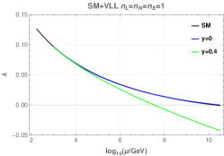
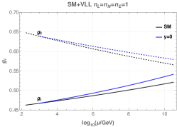
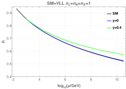
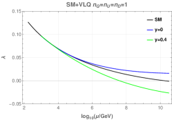
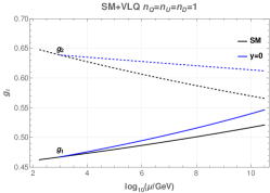
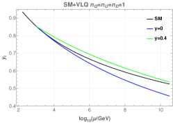
Figure 1: Running of $\lambda$ (left column), $g_{1}$ and $g_{2}$ (continuous and dashed lines respectively, middle column) and $y_{t}$ (right column) at 2-loop in the SM extended by VLF assuming $M_{F}=1$ TeV and varying VLF Yukawa coupling $y$.

In order to limit the number of free parameters, in our numerical analysis we make further simplifying assumptions, imposing that all Dirac masses of singlet and doublet VLF are the identical, $M_{F^{d}}=M_{F^{s}}=M_{F}$. Furthermore, we assume a single universal value of all VLF Yukawa couplings: $y_{F}=y$ for all new fermion multiplets. For the VLF masses, relying on the results of recent direct searches from ATLAS [42, 43, 44, 45, 46, 47] and CMS [48, 49, 50, 51, 52], we adopt the lower limit $M_{F}\gtrsim 1$ TeV. Too heavy VLF would lead to their effective decoupling and negligible modifications of the SM particles interactions (e.g. the triple Higgs coupling) and of observable phenomenology. Moreover, the cut-off scale $\Lambda$ must be larger than the heaviest particle in a given model, otherwise there would be no energy scale at which such model could be consistently defined. Thus, we consider masses of new particles, VLF and/or the scalar $S$, to be of the order $\mathcal{O}(1\div 10)$ TeV. Pushing $\Lambda$ to very large values significantly shrinks allowed model parameter space. For this reasons we consider $\Lambda=100\div 1000$ TeV as typical interesting range of the cut-off scale which we will use in most of our further considerations.

IV.1 SM extended with vector-like fermions only – case A

We illustrate the impact of VLF on the running of the Higgs quartic coupling $\lambda$ and EW vacuum stability given by (10) assuming $n=1$ (as we checked, behaviour of models with larger numbers of VLF families is qualitatively very similar, see also discussion in Section IV.5).

Plots in Fig. 1 show how varying VLF Yukawa couplings influences the running of $\lambda$, the gauge couplings $g_{1}$ and $g_{2}$ and the top Yukawa coupling $y_{t}$. Two main regimes can be distinguished depending on the magnitude of $y$:

1. VLF with small (or vanishing) Yukawa couplings.

They have positive impact on the stability of the EW vacuum, as compared to the SM, eventually even leading to the stability up to the Planck scale. This can be understood at the 1-loop level as follows. For $y=0$, VLF contributions affect directly the running of $g_{1}$ and $g_{2}$ gauge couplings (see Eq. (31)), which in turn leads to bigger values of $\beta_{\lambda}$ (see Eq. (29)). Adding VLQ multiplets leads to larger effects than adding VLL ones due to larger number of degrees of freedom, affecting RGE running through a bigger colour factor $N_{c}^{\prime}$ in Eq. (31). This effect in the case of $g_{1}$ is more model-dependent due to differences in hypercharges of quarks and leptons.

2. VLF with larger Yukawa couplings.

Increasing the VLF Yukawa couplings typically has negative impact on the stability of the EW vacuum. For these couplings bigger than some critical value the EW vacuum becomes unstable. This follows again from the 1-loop RGEs: the leading direct VLF contribution to the running of $\lambda$ is proportional to $(2\lambda-y_{F}^{2})y_{F}^{2}$ (see the first equation in (31)) which is positive for small values of $y_{F}^{2}$ but becomes negative for $y_{F}^{2}>2\lambda$. The negative contribution grows with increasing $y_{F}^{2}$ and very soon overcomes the indirect positive contribution mentioned in point 1 above. This effect is further strengthened by the positive contribution of VLF to $\beta_{y_{t}}$ which indirectly leads to bigger negative term in $\beta_{\lambda}$ proportional to $y_{t}^{4}$ (see the first equation in (29)).

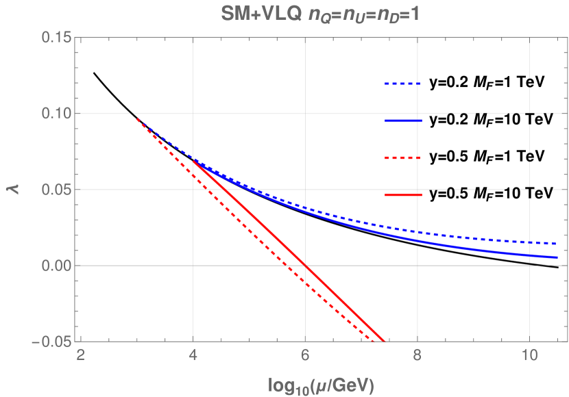
Figure 2: Running of $\lambda$ coupling for chosen values of $M_{F}$ and $y$. Black line indicates $\lambda$ behaviour in the SM.

The maximal value of the Yukawa coupling consistent with the stability condition (10) depends not only on the cut-off scale $\Lambda$ but also on the masses of VLF. Any effects from VLF are stronger when their masses are smaller because lighter particles modify RGEs starting from lower energy scales. This applies to both types of effects: those which improve and those which worsen stability of the EW vacuum. In Fig. 2 we illustrate this feature for two values of $y$ in scenario I with VLQ.

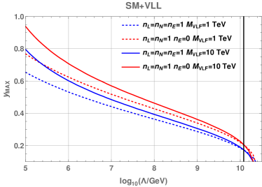
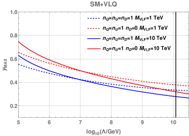
Figure 3: Maximal values of VLF Yukawa coupling for which stability condition is satisfied up to the given scale $\mu$. $M_{F}=1,10$ TeV. The vertical lines indicate the scale of the SM stability breakdown.

As we argued above, VLF with Yukawa couplings larger than some critical values have negative impact on the EW vacuum stability. The bigger are such couplings the lower is the energy scale at which $\lambda$ becomes negative. Thus, demanding $\lambda$ to be positive up to some chosen cut-off scale $\Lambda$ results in an upper limit on the Yukawa coupling, $y_{MAX}$, in a given model (we remind that by couplings without explicit scale-dependence we denote these couplings renormalized at the scale $\mu=M_{t}$).

Negative contributions to $\beta_{\lambda}$ from the VLF increase with the corresponding Yukawa couplings. Thus, the maximal value of the Yukawa coupling in a given model, $y_{MAX}$, is a decreasing functions of the cut-off scale $\Lambda$. Such dependence for scales above the $10^{9\div 10}$ GeV (close to the scale at which $\lambda$ becomes negative in the SM) is very different for VLL and VLQ models. In the case of VLL models $y_{MAX}$ drops very quickly to zero, while in VLQ models $y_{MAX}$ decreases very slowly. The reason for this difference follows from the impact of VLF with small Yukawa couplings on the RGE evolution of $\lambda$ discussed in the point 1 above (and illustrated in the upper row of plots in Fig. 1). Namely, VLL may improve the EW vacuum stability only sightly and only for very small Yukawa couplings, while addition of VLQ with not too large Yukawa couplings may stabilise the EW vacuum even up to the Planck scale.

A few examples of $y_{MAX}(\Lambda)$ for VLL and VLQ models are shown in Fig. 3. The biggest possible value of $y_{MAX}$, corresponding to the lowest cut-off scale considered in this paper, $\Lambda=100$ TeV, in scenarios I and II for VLL and VLQ models and for two values of $M_{F}$, are collected in Table 2.

	Scenario	$y_{MAX}$
		$M_{F}=1$ TeV	$M_{F}=10$ TeV
VLQ	$n_{Q}=n_{U}=n_{D}=1$	0.55	0.63
	$n_{Q}=n_{U}=1$ $n_{D}=0$	0.66	0.75
VLL	$n_{L}=n_{E}=n_{N}=1$	0.66	0.80
	$n_{L}=n_{N}=1$ $n_{N}=0$	0.77	0.94

Table 2: Maximal values of VLF Yukawa couplings allowed by the conditions (10)-(12) up to the scale $\Lambda=100$ TeV for two values of $M_{F}$.

Results presented in this Section show that in all considered scenarios the maximal values of VLF Yukawa couplings allowed by the EW stability condition are always relatively small, $y_{MAX}<1$, which, as we shall see later on, suggests limited range of phenomenological consequences of such BSM extensions which could be experimentally tested in near future. Many studies considering phenomenology of VLF models (e.g. [23, 26, 27, 28, 29, 30, 31, 32]) often require large values of VLF Yukawa couplings to produce significant observable effects. The present analysis shows that obtaining those effects may be not possible in perturbative models with stable EW vacuum.

The discussed above impact of VLF on the EW vacuum stability is in line with similar study [19], and we were able to reproduce their results. However, in our work we studied a wider set of VLF model scenarios, and focused more on their possible observable effects on phenomenology (which we discuss in Section V).

Our analysis obviously does not exhaust all possible VLF scenarios, but shows that the simple EW vacuum stability requirement strongly constraints allowed parameter space of such models. Testing VLF models with more complex pattern of different couplings would require case by case study, which is beyond the scope of this work.

IV.2 SM extended with real scalar singlet – case B

In order to explore the freedom of construction of VLF models and enlarge their allowed parameter space, we consider also SM extension containing also the real scalar singlet field, $S$, with a tree-level potential given in Eq. (7). We start with reviewing the theoretical constraints on SM extended by the real scalar singlet only.

The main effect of adding $S$ comes from the coupling between such scalar and the SM Higgs scalar, $\lambda_{HS}$, which gives a positive contribution to $\beta_{\lambda}$ (see the first equation in Eq. (32)). The singlet self-coupling, $\lambda_{S}$, also (indirectly) leads to bigger values of $\lambda$ via its positive contribution to $\beta_{\lambda_{HS}}$ (second equation in Eq. (32)). Thus, increasing scalar couplings, $\lambda_{HS}$ and $\lambda_{S}$, and/or decreasing $M_{S}$ result in larger values of $\lambda$ and so has positive impact on the stability of the EW vacuum. For example one gets its absolute stability up to the Planck scale for $M_{S}=1$ TeV, $\lambda_{S}=0$ and $\lambda_{HS}\gtrsim 0.3$.

However, increasing the values of $\lambda_{S}$ and $\lambda_{HS}$ too much may lead to the loss of perturbativity, i.e. condition(s) (11) and/or (12) may be violated below the chosen cut-off scale $\Lambda$. Fig. 4 shows regions on the $\lambda_{S}$-$\lambda_{HS}$ plane compatible with conditions (11)–(12) for chosen values of $\Lambda$ and the singlet mass $M_{S}$. As expected, increasing value of $M_{S}$ weakens the upper bound on $\lambda_{HS}$ while increasing $\lambda_{S}$ or $\Lambda$ makes this bound stronger.

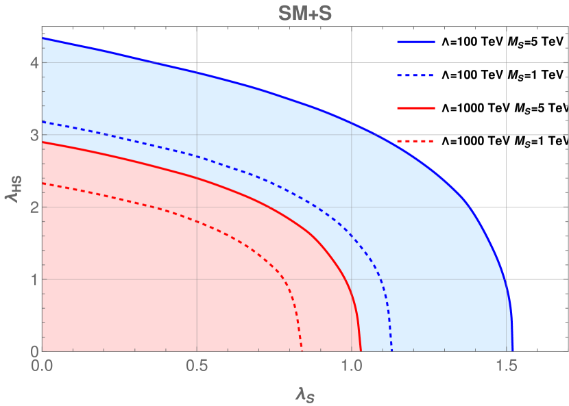
Figure 4: Parameter space of the SM extended by real singlet allowed by the perturbativity constraints up to $\Lambda=100,1000$ TeV with varying $M_{S}=1,5$ TeV.

Our approach provides new and independent way of studying allowed values of the parameters in the real scalar model and can be seen as complementary to the previous papers (e.g. [53, 54, 55]) by further constraining allowed parameter space of this model. It emphasises the importance of going beyond the naive study of perturbativity as given by the condition (11) by taking into account the differences between 1- and 2-loop contributions to the RGEs .

IV.3 SM extended with vector-like fermions and real scalar singlet – case C

Since, as discussed in the previous subsection, adding the scalar singlet to the model improves stability of the Higgs potential, it should also help to alleviate constraints on VLF Yukawa couplings summarised in Table 2. However, relaxing the constraints on $y_{MAX}$ in the presence of extra singlet scalar field should also take into account potential violation of perturbativity conditions (11) and (12) when increasing the values of new scalar couplings.

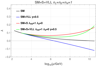
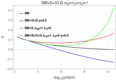
Figure 5: Running of $\lambda$ in a combined model SM+S+VLF for $M_{S}=1$ TeV and $M_{F}=1$ TeV.

In a model with the SM extended by the singlet scalar only (SM+S), all the conditions (10)-(12) are fulfilled in the SM+S model for values of $\lambda_{S}$ and $\lambda_{HS}$ which are not too large in order to avoid problems with perturbativity. As it turns out, adding VLF with Yukawa couplings big enough to have meaningful phenomenological effects further strengthens the constraints from the conditions (10)–(12), as VLF have both negative impact on the vacuum stability (see Section IV.1) and lead to stronger problems with perturbativity. The reason of the latter effect is obvious from Eq. (33): additional fermions give positive contribution to $\beta_{\lambda_{HS}}$ proportional to the sum of squares of their Yukawa coupling.

Impact of VLF on the RGE running of $\lambda$ is illustrated with examples in Fig. 5. The Higgs self-coupling $\lambda$ in the models with $S$ and VLF (green curves) is lower at low scales but bigger at high scales as compared to model without VLF (red curves). Both effects result in stronger constraints on singlet scalar couplings $\lambda_{S}$ and especially $\lambda_{HS}$. Stability condition (10) leads to lower bound on $\lambda_{HS}$ as function of $\lambda_{S}$, while perturbativity conditions (11) and (12) lead to corresponding upper bound. The impact of VLF on the allowed region for $\lambda_{HS}$ and $\lambda_{S}$ couplings is shown, depending on value of their Yukawa couplings, in Fig. 6 (for comparison, see corresponding plot without VLF shown in Fig. 4) and in Table 3

The allowed region in the $\lambda_{S}$-$\lambda_{HS}$ parameter space decreases with increasing VLF Yukawa couplings, eventually shrinking to the point defining its maximal allowed value $y_{MAX}$. Adding singlet $S$ to the theory may allow for maximal Yukawa couplings bigger by at most up to about 50% comparing to pure VLF models, as can be seen by comparing Tables 2 and 3.

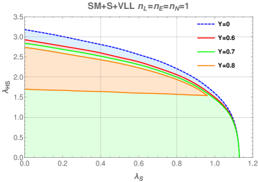
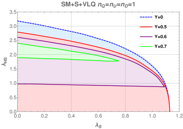
Figure 6: Allowed regions of the singlet scalar couplings in the SM extended by real singlet and VLF for the cut-off scale $\Lambda=100$ TeV with $M_{F}=M_{S}=1$ TeV and for different values of the VLF Yukawa coupling $Y$. The dashed blue contour is the same as in Fig. 4.

	SM+VLF		SM+S+VLF
Scenario	$y_{MAX}$		$\lambda_{HS}^{y_{MAX}}$	$y_{MAX}$	$\lambda_{HS}^{y_{MAX}}$	$y_{MAX}$
	$M_{F}=1$ TeV	$M_{F}=10$ TeV	$M_{F}=1$ TeV		$M_{F}=10$ TeV
$n_{Q}=n_{U}=n_{D}=1$	0.55	0.63	2.30	0.74	2.46	0.87
$n_{Q}=n_{U}=1$ $n_{D}=0$	0.65	0.74	2.55	0.91	2.66	1.07
$n_{L}=n_{E}=n_{N}=1$	0.65	0.79	2.59	0.93	2.71	1.16
$n_{L}=n_{N}=1$ $n_{N}=0$	0.76	0.92	2.77	1.11	2.85	1.40

Table 3: Maximal values of VLF Yukawa couplings $y_{MAX}$ allowed by the conditions (10)-(12), up to the scale $\Lambda=100$ TeV with $\Delta=0.4$ and the corresponding values of $\lambda_{HS}^{y_{MAX}}$ for which they can be achieved in the combined VLF + scalar model for $M_{S}=1$ TeV, $\lambda_{S}=0$ and two chosen values of $M_{F}$.

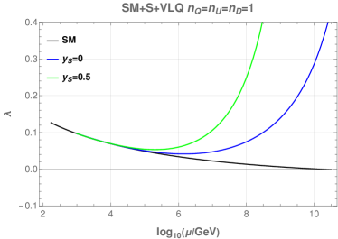
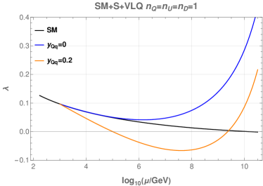
Figure 7: Running of $\lambda$ in a combined SM+S+VLF model for $M_{S}=1$ TeV and $M_{F}=1$ TeV with $y_{F}=0.5$, $\lambda_{HS}=1$ and $\lambda_{S}=0$, including VLF-$S$ Yukawa (left) and VLF-SMF (right) coupling.

IV.4 Models with additional VLF couplings

So far we assumed that there are no tree-level interactions between VLF and the singlet scalar $S$ or the SM fermions. As we discuss below, adding such couplings in general results in further shrinking of the allowed parameter space.

1. VLF and real scalar couplings.

The simplest way of including the VLF-$S$ couplings can be realised by adding the following terms to the Lagrangian:

$$-\sum_{i=1}^{n_{Q}}y_{QS}S\bar{Q}^{d}_{i}Q^{d}_{i}-\sum_{j=1}^{n_{U}}y_{US}S\bar{U}^{s}_{j}U^{s}_{j}-\sum_{k=1}^{n_{D}}y_{DS}S\bar{D}^{s}_{k}D^{s}_{k}$$ (13)

$$-\sum_{i=1}^{n_{L}}y_{LS}S\bar{L}^{d}_{i}L^{d}_{i}-\sum_{j=1}^{n_{N}}y_{NS}S\bar{N}^{s}_{j}N^{s}_{j}-\sum_{k=1}^{n_{E}}y_{ES}S\bar{E}^{s}_{k}E^{s}_{k}\,.$$

The presence of non-vanishing VLF-$S$ Yukawa couplings leads to even stronger bounds from perturbativity condition (11). The reason is as follows: $\beta_{\lambda_{HS}}$ has a positive contributions proportional to squares of Yukawa couplings present in Eq. (LABEL:eq:LSMSVLF:Coupled:1), increasing $\lambda_{HS}$ during evolution. This indirectly, via term proportional to $\lambda_{HS}^{2}$ in $\beta_{\lambda}$ (see eq. (32)), leads to a faster growth of $\lambda$. Such effect is illustrated in the left plot of Fig. 7 where for simplicity, we assumed all new Yukawa couplings to be equal - $y_{XS}\equiv y_{S}$, $X=Q,U,D,L,N,E$. Fig. 7 shows how non-vanishing $y_{S}$ pushes $\lambda$ to larger values, implying more severe problems with perturbativity than in the case of $y_{S}=0$ and in consequence leading to smaller allowed maximal values of VLF-Higgs Yukawa coupling.

2. VLF and SM fermion couplings.

Similarly, we can write down Lagrangian terms corresponding to the interactions between VLF and SM fermions. Assuming for simplicity that the only non-vanishing couplings are between the third family of SM quarks ($q_{L}$, $t_{R}$ and $b_{R}$) and VLQ in the $n_{Q}=n_{U}=n_{D}=1$ scenario we get the following extra terms in the Lagrangian:

$$-y_{Qt}\left(\bar{Q}^{d}_{L}\tilde{\Phi}t_{R}+\text{h.c.}\right)-y_{Uq}\left(\bar{q}_{L}\tilde{\Phi}U^{s}_{R}+\text{h.c.}\right)$$ (14)

$$-y_{Qb}\left(\bar{Q}^{d}_{L}\Phi b_{R}+\text{h.c.}\right)-y_{Dq}\left(\bar{q}_{L}\Phi D^{s}_{R}+\text{h.c.}\right)\,.$$

Non-vanishing VLQ-SM quarks Yukawa couplings have similar impact of the allowed parameter space as ordinary VLF Yukawa couplings discussed earlier in this Section. They give additional negative contributions to $\beta_{\lambda}$ resulting in problems with vacuum stability more severe than in the SM or when VLF and SM fermions are not interacting. Example of effects of non-vanishing VLQ-SM quarks Yukawa couplings for a simple case where $y_{Qt}=y_{Uq}=y_{Qb}=y_{Dq}=y_{Qq}$ is presented in the right panel of Fig. 7. One can see that even relatively small values of these additional Yukawa couplings may destabilise the EW vacuum.

IV.5 Gauge couplings unification in models with VLF

Fulfilling the vacuum stability and perturbativity conditions (10)–(12) is obligatory for the theoretical consistency of any BSM model. However, one can also impose other, more optional, requirements on the considered model field content and coupling structure, in order to achieve additional advantages in its predictions. One such possible extra condition may concern gauge coupling unification.

Let us define scales $\mu_{ij}$ at which pairs of gauge couplings, $g_{i}$ and $g_{j}$, have equal values, i.e. when $\Delta g_{ij}\equiv g_{i}(\mu_{ij})-g_{j}(\mu_{ij})=0$. In the SM these three scales are quite different with $\mu_{23}$ bigger than $\mu_{12}$ by more than 3 orders of magnitude, thus there is no common point of unification of gauge couplings.

The idea of grand unification favours models for which all three scales $\mu_{ij}$ are close to each other. In addition, higher unification scales, at least of order $10^{15}$ GeV, are preferred in order to avoid too fast proton decay. It is interesting to check whether unification of the gauge couplings may be achieved in models with extra VLF multiplets modifying their RGE evolution (we do not consider models with scalar singlet here).

In Fig. 8 we show how the energy scales at which the gauge couplings may unify depend on the number of VLF multiplet families for $M_{F}=3$ TeV (we point out that VLF Yukawa $y$ has no impact on the running of gauge couplings at 1-loop). Closer look at the plots on those figures reveals the following (compare Section II for model classification):

• SM + VLL models (crosses in Fig. 8):

  • scenario I (top panel) and scenario III (bottom panel): gauge couplings convergence points become closer to each other with increasing $n$ but the intersection points move to lower energy scales;

  • scenario II (middle panel): gauge couplings converge closer to each other for $n=1,2$ but already for $n=3$ they start diverging;

• SM + VLQ models (circles in Fig. 8):

  • scenario I (top panel): the $\Delta g_{23}=0$ point is above the Planck scale already for $n=1$;

  • scenario II (middle panel): gauge couplings converge closer to each other for $n=1,2$ but already for $n=3$ they start diverging, with all intersection points moving towards higher energy scales;

  • scenario III (bottom panel): for $n=1$ couplings converge closer to each other than in the SM, but already for $n=2$ the $\Delta g_{12}=0$ point is above the Planck scale.

As we checked, varying VLF mass $M_{F}$ between 1 TeV and 10 TeV does not make significant difference, general picture and conclusions remain the same.

Based on the discussion above, one can see that VLQ scenario II with $n=2$ (to a lesser extent also $n=1,3$) and scenario III with $n=1$ are the most promising ones for the idea of grand unification of gauge couplings in VLF models. All other cases are disfavoured due to different reasons. All VLL scenarios I, II and III with not too large $n$ have a positive impact on unification of couplings when compared to the SM. However, the corresponding unification scales are too low. The VLQ scenario I has a negative impact on unification and already for $n=2$, $g_{2}$ and $g_{3}$ couplings meet above the Planck scale. The situation is similar for the VLQ scenario III with $n\geq 2$.

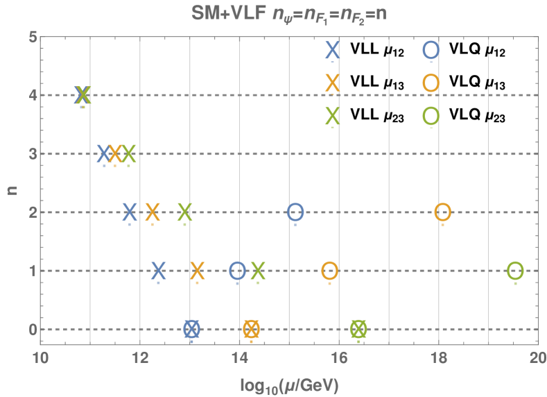
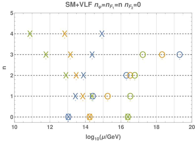
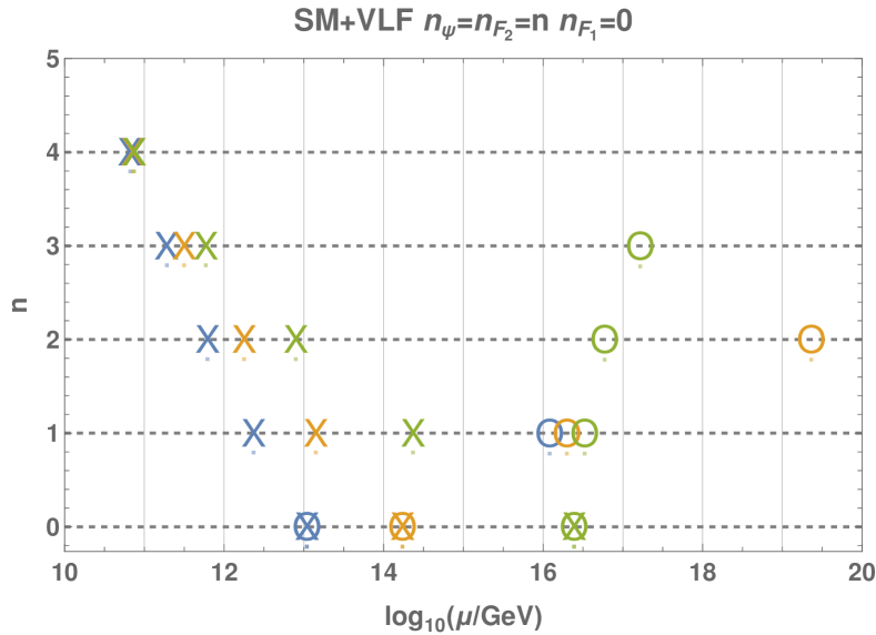
Figure 8: Energy scales $\mu_{ij}$ at which pairs of running gauge couplings have equal values in models with $n$ families of VLL (crosses) of VLQ (circles) with $M_{F}=3$ TeV. The 2-loop RGEs were used. $n_{\psi}\in\{n_{Q},n_{L}\}$, $n_{F_{1}}\in\{n_{U},n_{N}\}$ and $n_{F_{2}}\in\{n_{D},n_{E}\}$.

	SM+VLL	SM+VLQ
Scenario I	$n_{L}^{max}=4$	$n_{Q}^{max}=2$
Scenario II	$n_{L}^{max}=12$	$n_{Q}^{max}=3$
Scenario III	$n_{L}^{max}=4$	$n_{Q}^{max}=3$

Table 4: Maximal number of allowed VLF multiplet families based on the perturbativity conditions.

Models with large cut-off scales and big number of VLF multiplets are disfavoured not only from the point of view of possible unification of gauge couplings but also by perturbativity conditions (11) and (12). New fermions give positive contributions to the gauge coupling $\beta$-functions. Too many fermions lead to too fast grow of (at least some of) gauge couplings. Demanding the perturbativity up to the Planck scale gives upper bounds on the number of VLF multiplets presented in Table 4.

An additional remark concerning models with VLL is in order here. As we discussed in Sec. IV.1, EW vacuum in such models becomes unstable at scales above about $10^{9\div 10}$ GeV. Therefore, it is reasonable to consider much bigger cut-off scales only if the singlet scalar $S$ with suitable couplings is also added to the model, improving its stability. The singlet does not change the RGEs for the gauge couplings so the results presented in this Section are valid for SM+S+VLL models.

V Phenomenological consequences

As discussed in Section IV, the interplay between stability condition (10), and perturbativity conditions (11), (12) leaves surprisingly small allowed parameter space for the VLF models. Inclusion of a real scalar weakens somewhat the upper bounds on the values of VLF Yukawa couplings but as we shall show, these couplings are still not sufficient to justify expectations of rich phenomenology. In fact, the consequences which could be experimentally tested in near future are quite limited. We will focus on two examples of possible phenomena, namely double Higgs boson production and electroweak phase transition.

V.1 Double Higgs boson production

The enhancement of the double Higgs production cross section in models with new VLF multiplets and heavy scalar $S$ can occur by modification of the triple Higgs coupling or VLQ contributions to the box and triangle gluon fusion diagrams of Fig. 9. We denote differences between cross sections for the gluon fusion processes of single and double Higgs boson production in the SM and its extensions as:

$$K_{\text{final}}^{X}=\frac{\sigma^{SM+X}_{\text{ggF}}(pp\rightarrow\text{final})-\sigma^{SM}_{\text{ggF}}(pp\rightarrow\text{final})}{\sigma^{SM}_{\text{ggF}}(pp\rightarrow\text{final})}\,,$$ (15)

where $X$ is either $S$ or VLF, and “final” state can be $H$ for single and $HH$ for double Higgs production. From the experimental point of view we are interested in scenarios which predict significant enhancement of $K^{X}_{HH}$ while keeping $K^{X}_{H}$ within present experimental bounds.

Figure 9: Diagrams contributing to the double Higgs production via gluon fusion. Internal fermion lines indicated by $Q$ can be either SM quarks or VLQ multiplets. Black dot indicates triple Higgs coupling $\lambda_{3}$.

1. Modification of the triple Higgs coupling.

Interactions of the Higgs scalar with new particles can modify the triple Higgs coupling $\lambda_{3}$ which, if sizeable, may directly impact double Higgs boson production. This coupling is defined as:

$$\lambda_{3}\equiv \left.\frac{d^{3}\left(V_{0}(H,0)+V_{0}^{CW}(H,0)\right)}{dH^{3}}\right|_{H=v}$$ (16)

$$\equiv \lambda_{3}^{SM}+\Delta\lambda_{3}^{BSM}\equiv\lambda_{3\text{,tree}}^{SM}+\Delta\lambda_{3}^{SM}+\Delta\lambda_{3}^{BSM}\,,$$

with tree level potential given by Eq. (7) and its Coleman-Weinberg part by Eq. (34). The current allowed $95\%$ confidence level intervals for the trilinear Higgs coupling modifier $\kappa_{\lambda_{3}}=\lambda_{3}/\lambda_{3}^{SM}$ still leave a lot of room for the BSM physics and read:

$$\kappa_{\lambda_{3}} \in [-0.4,6.3],~{}\text{ATLAS~{}\cite[cite]{[\@@bibref{Number}{ATLAS:2022jtk}{}{}]}},$$

$$\kappa_{\lambda_{3}} \in [-1.24,6.49],~{}\text{CMS~{}\cite[cite]{[\@@bibref{Number}{CMS:2022dwd}{}{}]}}.$$ (17)

Corrections to the leading tree level contribution $\lambda_{3,\text{tree}}^{SM}=3M_{H}^{2}/v$ predicted by the SM can be classified as follows.

• Leading SM one-loop top-quark induced contribution:

  $$\Delta\lambda_{3}^{SM}\approx-\frac{3M_{t}^{4}}{v^{3}\pi^{2}}.$$ (18)

• Leading one-loop real scalar singlet induced contribution:

  $$\Delta\lambda_{3}^{S}\approx\frac{\lambda_{HS}^{3}v^{3}}{32\pi^{2}M_{S}^{2}}.$$ (19)

• Loop contributions from heavy VLF multiplets:

  $$\Delta\lambda_{3}^{VLF}\approx n_{F_{1}}\frac{N_{c}^{\prime}v^{3}y_{F_{1}}^{6}}{8\pi^{2}M_{F_{1}}^{2}}+n_{F_{2}}\frac{N_{c}^{\prime}v^{3}y_{F_{2}}^{6}}{8\pi^{2}M_{F_{2}}^{2}},$$ (20)

  where $N_{c}^{\prime}$ is the number of colours of VLF multiplets and one should sum over $n_{F_{1}}\in\{n_{U},n_{N}\}$, $n_{F_{2}}\in\{n_{D},n_{E}\}$ and $y_{F_{1}}\in\{y_{U},y_{N}\}$, $y_{F_{2}}\in\{y_{D},y_{E}\}$.

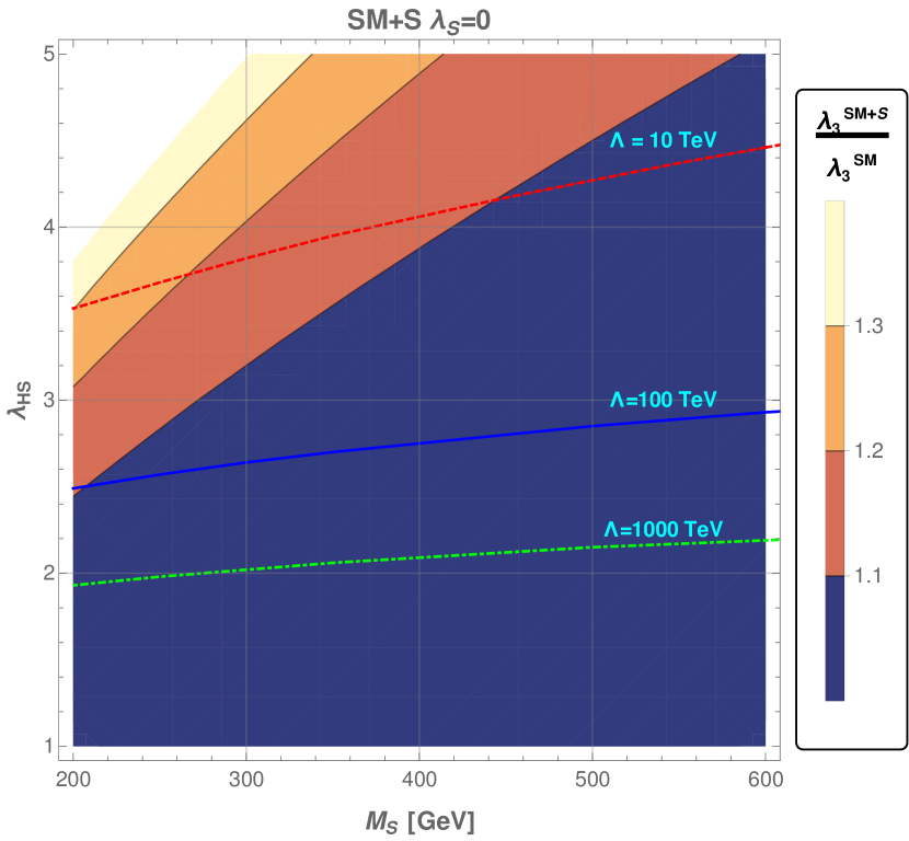
Figure 10: Contours of relative triple Higgs coupling enhancement in the SM extended by real singlet. Red-dashed, blue-solid and green-dot-dashed lines indicate maximal value of $\lambda_{HS}$ allowed by the perturbativity constraints up to, respectively, $\Lambda=10,100,1000$ TeV with $\Delta=0.4$ (compare eq. (12)).

Effects of the scalar singlet are presented in Fig. 10 which shows the corresponding relative enhancement of the triple Higgs coupling, $\kappa_{\lambda_{3}}^{SM+S}=\lambda_{3}^{SM+S}/\lambda_{3}^{SM}$. The contours of maximal allowed values of $\lambda_{HS}$ for chosen cut-off scales $\Lambda$ are obtained using perturbativity conditions (10)– (12).

For the cut-off scale of 100 TeV or lower, the enhancement of $\lambda_{3}$ from scalar singlet contributions is at most $\sim 10\%$ for $M_{S}\geq 200$ GeV, leading to a moderate, at most $K^{S}_{HH}\approx-8\%$, decrease of the double Higgs production cross section (which is due to destructive interference between the box and triangle diagrams of Fig. 9).

Addition of VLF also has some impact on $\lambda_{3}$, however, this effect is very small. We can estimate its maximal possible value by using numbers from Table 3 and plugging them into the Eq. (20). As a result, we get negligible contributions with $|\Delta\lambda_{3}^{VLF}/\lambda_{3}^{SM}|\ll 1\%$ for all considered cases, leaving no chance for significant triple Higgs coupling modification by VLF fields only.

2. VLQ loop contributions.

Apart from modifying the triple Higgs boson coupling $\lambda_{3}$, heavy VLQ may impact double Higgs boson production through the box and triangle loop gluon fusion diagrams presented in Fig. 9. Considering such corrections, one should take into account that loop contributions to the double and single Higgs boson production are closely related, the Feynman diagrams for the latter can be obtained from Fig. 9 by replacing one of the external Higgs fields by the VEV insertion. As a consequence, all relevant amplitudes are proportional to the same combination of VLQ parameters:

$$\mathcal{M}_{gghh}^{VLQ\triangle}\propto\mathcal{M}_{gghh}^{VLQ\Box}\propto\mathcal{M}_{ggh}^{VLQ}\propto n_{U}\frac{y_{U}^{2}}{M_{U}^{2}}+n_{D}\frac{y_{D}^{2}}{M_{D}^{2}}$$ (21)

Therefore, apart from theoretical constraints considered already in this work, another important source of limits on VLQ model parameters comes from the current limits on the single Higgs production. Available experimental data [70] puts strong constraint, at around $10\%$ at $68\%$ CL and around $18\%$ at $95\%$ CL, on the deviations of the single Higgs boson production rate via gluon fusion from its SM value. This condition may (depending on the choice of $\Delta$ in (12)) lead to stronger constraints on the maximal values of VLF Yukawa couplings then listed in Table 3, as illustrated in Table 5.

SM+VLQ	$y^{RGE}_{MAX}$	$y^{H}_{MAX}$	$K_{HH}^{VLQ}$	$y^{RGE}_{MAX}$	$y^{H}_{MAX}$	$K_{HH}^{VLQ}$
	$68\%$ CL			$95\%$ CL
$n_{Q}=n_{U}=n_{D}=1$	0.74	0.65	$+8.4\%$	0.74	0.89	$+11.3\%$
$n_{Q}=n_{U}=n_{D}=2$	0.60	0.46	$+8.2\%$	0.60	0.63	$+15.0\%$
$n_{Q}=n_{U}=n_{D}=3$	0.50	0.37	$+8.3\%$	0.50	0.51	$+15.5\%$
$n_{Q}=n_{U}=1$ $n_{D}=0$	0.91	0.92	$+8.2\%$	0.91	1.26	$+8.2\%$
$n_{Q}=n_{U}=2$ $n_{D}=0$	0.74	0.65	$+8.4\%$	0.74	0.89	$+11.3\%$
$n_{Q}=n_{U}=3$ $n_{D}=0$	0.65	0.53	$+8.2\%$	0.66	0.73	$+13.5\%$

Table 5: Maximal enhancement of the double Higgs production cross section from VLQ loop gluon fusion diagrams for $M_{F}=1$ TeV. $y^{RGE}_{MAX}$ and $y^{H}_{MAX}$ indicate maximal values allowed respectively by perturbativity and by single Higgs production constraints (the latter at CL=68% or 95% [70]). In each case bold font indicates stronger constraint that is taken into account.

Table 5 shows that the enhancement of the double Higgs production rate due to the VLQ loop contributions, $K_{HH}^{VLQ}$, within the parameter space obtained in this work, is always small (at most $\sim 15\%$). Even such minor enhancement should be considered as optimistic scenario. As discussed before, in models with scalar singlet this positive contribution may be in addition compensated by scalar contribution to the triple Higgs coupling. Increasing $M_{F}$ can also only further suppress the VLF effects. Finally, effects of increasing number of VLF multiplets can be deduced from the form of the amplitudes in (21) - for example, assuming identical masses for all multiplets, case with $n=1$ and some value of $Y$ is equivalent to $n=N$ with $Y\to Y/\sqrt{N}$, so that the corresponding bounds on $K_{HH}^{VLQ}$ are not much affected by varying $n$ (as can be seen in the 4th column of Table 5).

Comparing numbers in Table 5 with still rather lax current experimental constraints on the Higgs boson pair production at $95\%$ confidence level:

$$\sigma(pp\rightarrow HH) < 2.4\times\sigma^{SM}(pp\rightarrow HH),~{}\text{ATLAS~{}\cite[cite]{[\@@bibref{Number}{ATLAS:2022jtk}{}{}]}}\,,$$

$$\sigma(pp\rightarrow HH) < 3.4\times\sigma^{SM}(pp\rightarrow HH),~{}\text{CMS~{}\cite[cite]{[\@@bibref{Number}{CMS:2022dwd}{}{}]}}\,,$$ (22)

one can conclude that adding vector-like multiplets to the SM likely cannot affect the double Higgs production in a way which could be experimentally observed at present or in the foreseeable future.

V.2 Electroweak phase transition

The one-loop effective potential in the SM with additional singlet scalar field (for review see e.g. [77]) reads:

$$V_{\mathrm{eff}}(H,S,T)=V_{0}(H,S)+V_{CW}(H,S)+V_{T}(H,S,T)\,.$$ (23)

with $V_{0}$ a tree-level potential (7), $V_{CW}$ the one-loop correction known also as the Coleman-Weinberg potential [78] and $V_{T}$ the finite temperature contribution (for further details see Appendix B).

Models are considered to be interesting in the context of baryogenesis if they allow for a strong enough first order phase transition. In general, a 1st order electroweak phase transition may occur in the presence of a barrier in the effective Higgs potential separating two degenerate minima at $h=0$ and $h=v_{C}$ (here, $v_{C}$ is the VEV of the Higgs field at the critical temperature, $T=T_{C}$). The phase transition is considered strong if the following condition is satisfied:

$$\xi=\frac{v_{C}(T_{C})}{T_{C}}\gtrsim(0.6\div 1.0).$$ (24)

1. EWPT with real scalar singlet.

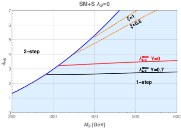
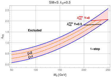
Figure 11: Shaded regions show parts of the parameter space allowing for the 1-step (left panel) and 2-step (right panel) EWPT in the SM extended by a singlet scalar. The orange dashed lines indicate strength of the EWPT $\xi=0.6$ or $\xi=1$ (1-step) and $\xi=1$ or $\xi=2$ (2-step). The red and black lines indicate maximal values of $\lambda_{HS}$ allowed by the perturbativity constraints up to $\Lambda=100$ TeV for two values of the VLF Yukawa couplings. Values of $\lambda_{S}$ were chosen as 0 and 0.5 for the 1- and 2-step transition, respectively.

In the real scalar model with the tree-level potential given by Eq. (7), depending on the values of the scalar sector couplings and masses, we can get either 1- or 2-step EWPT. The former takes place when the system moves from the high-temperature minimum with $\left<H\right>=\left<S\right>=0$ to the standard EW vacuum with $\left<H\right>\neq 0$, $\left<S\right>=0$. The latter is realised if for some range of temperatures the minimum of the effective potential is located at $\left<H\right>=0$, $\left<S\right>\neq 0$.

• 1-step EWPT is realised if $\mu_{S}^{2}>0$. This region is not affected by the value of $\lambda_{S}$, therefore we choose $\lambda_{S}=0$ in order to maximise the allowed value of $\lambda_{HS}$ coupling. The allowed parameter space for the 1-step EWPT is presented on the left panel in Fig. 11. The blue line indicates the boundary between 1- and 2-step regions. The red and black lines indicate maximal allowed values of $\lambda_{HS}(M_{S})$ obtained with constraints (11) and (12) assuming $\Lambda=100$ TeV for two values of the VLF Yukawa couplings. The orange dashed lines indicate values of $\lambda_{HS}(M_{S})$ corresponding to the strength of the EWPT, $\xi$ equal 0.6 and 1.0. As one can note, the region for which $\xi\geq 0.6$ in the singlet scalar extension is basically excluded in comparison e.g. with corresponding area presented in [53]. This follows from our more careful treatment of perturbativity conditions.

• 2-step EWPT may be realised if $\mu_{S}^{2}<0$ with further condition guaranteeing that at zero temperature the EW vacuum corresponds to the global minimum of the potential:

  $$V_{0}(v,0)<V_{0}(0,w)\,,$$ (25)

  which can be translated to the bounds on $\lambda_{HS}$. A 2-step EWPT is possible if:

  $$2\frac{M_{S}^{2}}{v^{2}}\leq\lambda_{HS}\leq 2\frac{M_{S}^{2}}{v^{2}}+\sqrt{2}\frac{M_{H}\sqrt{\lambda_{S}}}{v}\,.$$ (26)

  The allowed 2-step region is indicated by the red colour on the right plot in Fig. 11. The lower and upper limits from the Eq. (26) for $\lambda_{S}=0.5$ are indicated by the blue lines. The choice of this particular value of $\lambda_{S}$ allows for reasonably large $\lambda_{HS}$ while still leaving space for the 2-step EWPT to occur. The red line, as in the case of 1-step transition, show the maximal possible values of $\lambda_{HS}$.

2. EWPT with vector-like fermions.

In principle VLF can also affect the mechanism of the EWPT through thermal and loop corrections to the effective potential (see Appendix B). Fermions do not contribute much to inducing potential barrier for the Higgs field, contrary to the case of bosons which in general lead to cubic terms in the potential in the high temperature expansion of thermal effects. However, in the case in which the critical temperature is much lower than fermion masses, the small temperature expansion is more suitable. In the latter case, which fits very well the scope of this work in which VLF are relatively heavy, the leading contribution to the thermal potential is similar for fermions and bosons. This could potentially lead to non-trivial impact of VLF on EWPT and thermal history of the Universe (see e.g. [23, 23]).

However, because of strong constraints on the values of the VLF Yukawa couplings, discussed in Section IV, the actual impact of these particles on the EWPT is very limited. For the maximal allowed values of $y_{F}$ in SM+VLF models, presented in Table 3, we obtained $\xi_{SM+VLF}$ quite close to $\xi_{SM}$. Addition of the real singlet scalar allows for slightly larger maximal values of $y_{F}$, see Table 3, but these larger values are not sufficient to have any significant impact on the EWPT, so $\xi_{SM+S+VLF}\approx\xi_{SM+S}$. We checked that changes of $\xi$ due to VLF are at most of the order $\mathcal{O}(10\%)$.

VI Summary and outlook

In this work we studied consequences of extending the Standard Model by adding vector-like fermions and/or a real scalar singlet for the stability of the electroweak vacuum, for perturbativity of the model couplings and for possible unification of the gauge couplings. We divided our discussion into analysis of three broader model classes with different sets of extra fields: only VLF; only a singlet scalar; both VLF and a scalar. Further, the VLF models were classified into three types based on numbers of extra multiplets with different transformation properties with respect to the SM gauge group. In order to study the most generic features of discussed models, for simplicity we assumed equal masses and couplings of VLF multiplets, therefore we did not discuss any effects which could be related to flavor-like structure of their parameters.

We defined a set of theoretical conditions, summarised by equations (10)–(12), which play a pivotal role in deriving the results of this work. These conditions come solely from the stability and perturbativity requirements of the considered models. The primary strategy in our work was to implement the 2-loop RGEs and derive constraints from the resulting coupling evolution. In addition, we incorporated in our discussion also various experimental bounds, coming from trilinear Higgs coupling, Higgs production cross-section, bounds on masses of VLF and the real scalar field.

We obtained strong upper bounds on magnitude of VLF Yukawa couplings. The precise limits on such couplings, $y_{MAX}$, vary with details of models and with the assumed cut-off scale $\Lambda$ up to which the theoretical constraints should be fulfilled. However, in all cases we get $y_{MAX}<1$ for all considered scenarios if $\Lambda\geq 100$ TeV.

In terms of EW stability, the scalar singlet extension of the SM offers better prospects. The stability of the EW vacuum improves with increasing the singlet scalar couplings, $\lambda_{HS}$ and $\lambda_{S}$. However, the model loses perturbativity when scalar couplings become too large. Models with both VLF families and the real scalar have typically less problems with the EW vacuum stability than models with only VLF. On the other hand, interplay between VLF and the scalar results in bigger problems with the perturbativity as compared to the situation when only the scalar is added to the SM. In general, our analysis shows that the upper bounds on the VLF Yukawa couplings can be somewhat relaxed due to the presence of the singlet scalar, however such enhancement of $y_{MAX}$ is never larger than about 50%.

Finally, we analysed the implications of the constrained parameter space on the phenomenology of the double Higgs boson production and the electroweak phase transition. Adding scalar singlet to SM can increase somewhat the triple Higgs coupling $\lambda_{3}$ enhancing the single Higgs production but simultaneously suppressing the double Higgs production rate. Adding VLF fields have negligible effect on $\lambda_{3}$ but may affect the Higgs boson pair production via contribution to the triangle and box loops in the amplitude. Still, within the allowed parameter space, the VLF loops may enhance the double Higgs production rate by at most $15\%$, thus their impact is very limited and impossible to observe with current or achievable in near future experimental accuracy.

We demonstrated that the parameter space of the SM+S model is heavily constrained, leaving very little room for a strong first order EWPT. We showed also that addition of VLF with Yukawa couplings satisfying the stability and perturbativity conditions has again very little impact on the EWPT. Thus, the strong first order phase transition in the SM with only VLF added (no extra scalars) can not be realised.

The results presented in this work provide an independent set of constraints for models that extend the Standard Model with vector-like fermions and a scalar field. We believe these constraints are an important addition to the existing analyses, in the context of the considered models. Furthermore, the methodology employed here can be readily applied to study other theoretical frameworks beyond the specific scenarios explored in the current work.

Appendix A RGEs for models with extended scalar and vector-like sectors

Below we present 1-loop RGEs for all of the relevant couplings in the model considered in the paper, $\kappa_{i}=(\lambda,y_{t}^{2},g_{1}^{2},g_{2}^{2},g_{3}^{2},y_{F}^{2},\lambda_{HS},\lambda_{S})$, separated into the parts corresponding to various sectors of the theory which (alongside 2-loop contributions which are to lengthy to be displayed), were obtained using SARAH package [73] and validated using RGBeta [74].

$$\beta^{(1)}_{\kappa_{i}} =\beta^{SM(1)}_{\kappa_{i}}+\beta^{VLF(1)}_{\kappa_{i}}+\beta^{S(1)}_{\kappa_{i}}+\beta^{VLF(1)\times S(1)}_{\kappa_{i}}$$ (27)

with:

$$\frac{d\kappa_{i}(\mu)}{d\ln\mu}=\beta_{\kappa_{i}}\left(\kappa_{j}(\mu)\right)\equiv\beta_{\kappa_{i}}$$ (28)

A.1 SM sector

$$\beta_{\lambda}^{SM(1)} =\frac{1}{16\pi^{2}}\left[\frac{9}{8}\left(\frac{3}{25}g_{1}^{4}+g_{2}^{4}+\frac{2}{5}g_{1}^{2}g_{2}^{2}\right)\right.$$ (29)

$$\left.\qquad\qquad-6y_{t}^{4}+24\lambda^{2}+12y_{t}^{2}\lambda-\frac{9}{5}g_{1}^{2}\lambda-9g_{2}^{2}\lambda\right]$$

$$\beta_{y_{t}^{2}}^{SM(1)} =\frac{y_{t}^{2}}{16\pi^{2}}\left[9y_{t}^{2}-\frac{17}{10}g_{1}^{2}-\frac{9}{2}g_{2}^{2}-16g_{3}^{2}\right]$$

$$\beta_{g_{1}^{2}}^{SM(1)} =\frac{1}{16\pi^{2}}\left[\frac{41}{5}g_{1}^{4}\right],$$

$$\beta_{g_{2}^{2}}^{SM(1)} =\frac{1}{16\pi^{2}}\left[-\frac{19}{3}g_{2}^{4}\right],$$

$$\beta_{g_{3}^{2}}^{SM(1)} =\frac{1}{16\pi^{2}}\left[-14g_{3}^{4}\right].$$

A.2 Vector-like fermion sector

$$\beta_{\lambda}^{VLF(1)} =\frac{1}{16\pi^{2}}\left[2n_{F_{1}}N_{c}^{\prime}\left(4y_{F_{1}}^{2}\lambda-2y_{F_{1}}^{4}\right)\right.$$ (30)

$$\left.\qquad\qquad+2n_{F_{2}}N_{c}^{\prime}\left(4y_{F_{2}}^{2}\lambda-2y_{F_{2}}^{4}\right)\right],$$

$$\beta_{y_{t}^{2}}^{VLF(1)} =\frac{y_{t}^{2}}{16\pi^{2}}\left[4N_{c}^{\prime}\left(n_{F_{1}}y_{F_{1}}^{2}+n_{F_{2}}y_{F_{2}}^{2}\right)\right],$$

$$\beta_{g_{1}^{2}}^{VLF(1)} =\frac{g_{1}^{4}}{16\pi^{2}}\left[\frac{8}{5}N_{c}^{\prime}\left(2n_{\psi}Y_{W_{\psi}}^{2}+n_{F_{1}}Y_{W_{F1}}^{2}+n_{F_{2}}Y_{W_{F2}}^{2}\right)\right],$$

$$\beta_{g_{2}^{2}}^{VLF(1)} =\frac{1}{16\pi^{2}}\left[\frac{4}{3}N_{c}^{\prime}n_{\psi}g_{2}^{4}\right],$$

$$\beta_{g_{3}^{2}}^{VLF(1)} =\frac{1}{16\pi^{2}}\left[\frac{4}{3}n_{3}g_{3}^{4}\right],$$

$$\beta_{y_{F_{1}}^{2}}^{VLF(1)} =\frac{y_{F_{1}}^{2}}{16\pi^{2}}\left[3y_{F_{1}}^{2}+4n_{F_{1}}N_{c}^{\prime}y_{F_{1}}^{2}+6y_{t}^{2}-16\hat{n}_{F}^{VLQ}g_{3}^{2}\right.$$ (31)

$$\qquad\qquad-\frac{9}{2}g_{2}^{2}-\frac{18}{5}g_{1}^{2}\left(Y_{W_{H}}^{2}+2Y_{W_{F1}}Y_{W_{\psi}}\right)$$

$$\left.\qquad\qquad+\Delta_{n_{F_{1}},n_{F_{2}}}\left(5+4n_{F_{1}}N_{c}^{\prime}\right)y_{F_{2}}^{2}\right],$$

$$\beta_{y_{F_{2}}^{2}}^{VLF(1)} =\frac{y_{F_{2}}^{2}}{16\pi^{2}}\left[3y_{F_{2}}^{2}+4n_{F_{2}}N_{c}^{\prime}y_{F_{2}}^{2}+6y_{t}^{2}-16\hat{n}_{F}^{VLQ}g_{3}^{2}\right.$$

$$\qquad\qquad-\frac{9}{2}g_{2}^{2}-\frac{18}{5}g_{1}^{2}\left(Y_{W_{H}}^{2}+2Y_{W_{F2}}Y_{W_{\psi}}\right)$$

$$\left.\qquad\qquad+\Delta_{n_{F_{1}},n_{F_{2}}}\left(5+4n_{F_{2}}N_{c}^{\prime}\right)y_{F_{1}}^{2}\right]\,,$$

where $N_{c}^{\prime}$ is a number of colours of VLF, $n_{F_{1}}\in\{n_{U},n_{N}\}$, $n_{F_{2}}\in\{n_{D},n_{E}\}$, $n_{\psi}\in\{n_{Q},n_{L}\}$, $n_{3}=2n_{Q}+n_{U}+n_{D}$, $y_{F_{1}}\in\{y_{U},y_{N}\}$, $y_{F_{2}}\in\{y_{D},y_{E}\}$, $Y_{W_{H}}=1/2$, $Y_{W_{\psi}}\in\{Y_{W_{Q}},Y_{W_{L}}\}$, $Y_{W_{F1}}\in\{Y_{W_{U}},Y_{W_{N}}\}$, $Y_{W_{F2}}\in\{Y_{W_{D}},Y_{W_{E}}\}$.

A.3 Real scalar sector

$$\beta_{\lambda}^{S(1)} =\frac{1}{16\pi^{2}}\left[\frac{1}{2}\lambda_{HS}^{2}\right]$$ (32)

$$\beta_{\lambda_{HS}}^{S(1)} =\frac{\lambda_{HS}}{16\pi^{2}}\left[12\lambda+6\lambda_{S}+4\lambda_{HS}+6y_{t}^{2}-\frac{3}{2}g_{1}^{2}-\frac{9}{2}g_{2}^{2}\right]$$

$$\beta_{\lambda_{S}}^{S(1)} =\frac{1}{16\pi^{2}}\left[2\lambda_{HS}^{2}+18\lambda_{S}^{2}\right].$$

A.4 Vector-like fermion $\times$ real scalar sector

$$\beta_{\lambda_{HS}}^{VLF(1)\times S(1)} =\frac{\lambda_{HS}}{16\pi^{2}}\left[4N_{c}^{\prime}(n_{F_{1}}y_{F_{1}}^{2}+n_{F_{2}}y_{F_{2}}^{2})\right].$$ (33)

Appendix B Effective potential

One-loop effective potential is given schematically in Eq. 23. Coleman-Weinberg part of the potential in on-shell renormalization scheme with cutoff regularisation reads:

$$V_{CW}(H)=\sum_{k} \frac{r_{k}N_{k}}{64\pi^{2}}\left(2M_{k}^{2}(H)M_{k}^{2}(v)\right.$$ (34)

$$\left.+M_{k}^{4}(H)\left(\log\frac{M_{k}^{2}(H)}{M_{k}^{2}(v)}-\frac{3}{2}\right)\right)$$

$$-\frac{N_{F}}{64\pi^{2}}\sum_{i=1,2} n_{F_{i}}\left(M_{F_{i}}(H)^{4}\left(\log\frac{M_{F_{i}}(H)^{2}}{\mu_{R}^{2}}-\frac{3}{2}\right)\right.$$

$$\left.+C_{1}\phi^{2}+C_{2}\phi^{4}\right),$$

where we use the following notation:

$$k=(t,W,Z,h,S),\quad N_{k}=(12,6,3,1,1),$$ (35)

$$M_{k}(H)^{2}=M_{0,k}^{2}+a_{k}h^{2},\quad M_{0,k}^{2}=\left(0,0,0,-\mu^{2},~{}\mu_{S}^{2}\right),$$

$$a_{k}=\left(\frac{\lambda_{t}^{2}}{2},\frac{g^{2}}{4},\frac{g^{2}+g^{{}^{\prime}2}}{4},3\lambda,\frac{1}{2}\lambda_{HS}\right).$$

and

$$F=(VLQ,VLL), \quad N_{F}=(12,4)$$ (36)

$$n_{F_{1}}\in\{n_{U},n_{N}\}, \quad n_{F_{2}}\in\{n_{D},n_{E}\},$$

$$M_{F_{1(2)}}=M_{F}\pm\frac{\sqrt{2}}{2}y_{F}v,$$

and particle statistics related sign equals to $r_{k}=+(-)$ for bosons (fermions).

We assume renormalization conditions which ensure that Higgs mass and VEV remain the same as at the tree level, and that there is no explicit renormalization scale $\mu_{R}$ dependence in the effective potential (up to field independent term which can be cancelled by shifting potential by a constant, such that $V(\phi=0)=0$). They read as

$$\left.\frac{\partial}{\partial\phi}V_{CW}\right|_{\phi=v}=\left.0\qquad\frac{\partial^{2}}{\partial\phi^{2}}V_{CW}\right|_{\phi=v}=0.$$ (37)

First line of the equation (34) automatically satisfies conditions (37), whereas $C_{1}$ and $C_{2}$ in the second line are chosen to achieve the same outcome. Temperature corrections to the effective potential are given by:

$$V_{T}(H,S,T)= \sum_{k}\frac{N_{k}T^{4}}{2\pi^{2}}J_{r_{k}}\left(M_{k}(H,S)/T\right)$$

$$+N_{F}\sum_{i=1,2}\frac{n_{F_{i}}T^{4}}{2\pi^{2}}J_{-}\left(M_{F_{i}}(H,S)/T\right),$$ (38)

where the thermal functions $J_{\pm}(y)$ with $y=M/T$ are given by:

$$J_{\pm}(y)=\pm\int_{0}^{\infty}\mathrm{d}xx^{2}\log\left[1\mp e^{-\sqrt{x^{2}+y^{2}}}\right].$$ (39)

At $T\neq 0$, the field dependent scalar and longitudinal gauge boson masses get modified with thermal loop effects. They are added as $\Pi$ to the field dependent masses [79, 80],

$$\Pi_{H}(0) = \left(\frac{3g^{2}}{16}+\frac{g^{\prime 2}}{16}+\frac{\lambda}{2}+\frac{y_{t}^{2}}{4}+\frac{1}{2}\sum_{F}y_{F}^{2}+\frac{\lambda_{HS}}{24}\right)T^{2},$$

$$\Pi_{s}(0) = \left(\frac{1}{6}\lambda_{HS}+\frac{1}{4}\lambda_{S}\right)T^{2},$$

$$\Pi_{GB}^{L}(0) = \frac{11}{6}T^{2}\operatorname{diag}\left(g^{2},g^{2},g^{2},g^{\prime 2}\right).$$ (40)

References

- Chatrchyan et al. [2012] S. Chatrchyan et al. (CMS), Observation of a New Boson at a Mass of 125 GeV with the CMS Experiment at the LHC, Phys. Lett. B 716, 30 (2012), arXiv:1207.7235 [hep-ex] .
- Aad et al. [2012] G. Aad et al. (ATLAS), Observation of a new particle in the search for the Standard Model Higgs boson with the ATLAS detector at the LHC, Phys. Lett. B 716, 1 (2012), arXiv:1207.7214 [hep-ex] .
- Cheng et al. [2000] H.-C. Cheng, B. A. Dobrescu, and C. T. Hill, Electroweak symmetry breaking and extra dimensions, Nucl. Phys. B 589, 249 (2000), arXiv:hep-ph/9912343 .
- Arkani-Hamed et al. [2002] N. Arkani-Hamed, A. G. Cohen, E. Katz, and A. E. Nelson, The Littlest Higgs, JHEP 07, 034, arXiv:hep-ph/0206021 .
- Han et al. [2003] T. Han, H. E. Logan, B. McElrath, and L.-T. Wang, Loop induced decays of the little Higgs: H — gg, gamma gamma, Phys. Lett. B 563, 191 (2003), [Erratum: Phys.Lett.B 603, 257–259 (2004)], arXiv:hep-ph/0302188 .
- Cheng et al. [2006] H.-C. Cheng, I. Low, and L.-T. Wang, Top partners in little Higgs theories with T-parity, Phys. Rev. D 74, 055001 (2006), arXiv:hep-ph/0510225 .
- Kang et al. [2008] J. Kang, P. Langacker, and B. D. Nelson, Theory and Phenomenology of Exotic Isosinglet Quarks and Squarks, Phys. Rev. D 77, 035003 (2008), arXiv:0708.2701 [hep-ph] .
- Cacciapaglia et al. [2019] G. Cacciapaglia, A. Carvalho, A. Deandrea, T. Flacke, B. Fuks, D. Majumder, L. Panizzi, and H.-S. Shao, Next-to-leading-order predictions for single vector-like quark production at the LHC, Phys. Lett. B 793, 206 (2019), arXiv:1811.05055 [hep-ph] .
- Cacciapaglia et al. [2012] G. Cacciapaglia, A. Deandrea, L. Panizzi, N. Gaur, D. Harada, and Y. Okada, Heavy Vector-like Top Partners at the LHC and flavour constraints, JHEP 03, 070, arXiv:1108.6329 [hep-ph] .
- Aguilar-Saavedra et al. [2013] J. A. Aguilar-Saavedra, R. Benbrik, S. Heinemeyer, and M. Pérez-Victoria, Handbook of vectorlike quarks: Mixing and single production, Phys. Rev. D 88, 094010 (2013), arXiv:1306.0572 [hep-ph] .
- Ellis et al. [2014] S. A. R. Ellis, R. M. Godbole, S. Gopalakrishna, and J. D. Wells, Survey of vector-like fermion extensions of the Standard Model and their phenomenological implications, JHEP 09, 130, arXiv:1404.4398 [hep-ph] .
- Angelescu et al. [2016] A. Angelescu, A. Djouadi, and G. Moreau, Scenarii for interpretations of the LHC diphoton excess: two Higgs doublets and vector-like quarks and leptons, Phys. Lett. B 756, 126 (2016), arXiv:1512.04921 [hep-ph] .
- Arhrib et al. [2018] A. Arhrib, R. Benbrik, S. J. D. King, B. Manaut, S. Moretti, and C. S. Un, Phenomenology of 2HDM with vectorlike quarks, Phys. Rev. D 97, 095015 (2018), arXiv:1607.08517 [hep-ph] .
- Barducci and Panizzi [2017] D. Barducci and L. Panizzi, Vector-like quarks coupling discrimination at the LHC and future hadron colliders, JHEP 12, 057, arXiv:1710.02325 [hep-ph] .
- Arhrib et al. [2019] A. Arhrib, R. Benbrik, J. El Falaki, M. Sampaio, and R. Santos, Pseudoscalar decays to gauge bosons at the LHC and at a future 100 TeV collider, Phys. Rev. D 99, 035043 (2019), arXiv:1809.04805 [hep-ph] .
- Song and Yoon [2019] J. Song and Y. W. Yoon, decay of the elusive charged Higgs boson in the two-Higgs-doublet model with vectorlike fermions, Phys. Rev. D 100, 055006 (2019), arXiv:1904.06521 [hep-ph] .
- del Aguila et al. [1990] F. del Aguila, L. Ametller, G. L. Kane, and J. Vidal, Vector Like Fermion and Standard Higgs Production at Hadron Colliders, Nucl. Phys. B 334, 1 (1990).
- Cárcamo Hernández et al. [2023] A. E. Cárcamo Hernández, K. Kowalska, H. Lee, and D. Rizzo, Global analysis and LHC study of a vector-like extension of the Standard Model with extra scalars (2023), arXiv:2309.13968 [hep-ph] .
- Gopalakrishna and Velusamy [2019] S. Gopalakrishna and A. Velusamy, Higgs vacuum stability with vectorlike fermions, Phys. Rev. D 99, 115020 (2019), arXiv:1812.11303 [hep-ph] .
- Arsenault et al. [2023] A. Arsenault, K. Y. Cingiloglu, and M. Frank, Vacuum stability in the Standard Model with vectorlike fermions, Phys. Rev. D 107, 036018 (2023), arXiv:2207.10332 [hep-ph] .
- Cacciapaglia et al. [2017] G. Cacciapaglia, H. Cai, A. Carvalho, A. Deandrea, T. Flacke, B. Fuks, D. Majumder, and H.-S. Shao, Probing vector-like quark models with Higgs-boson pair production, JHEP 07, 005, arXiv:1703.10614 [hep-ph] .
- Cheung et al. [2021] K. Cheung, A. Jueid, C.-T. Lu, J. Song, and Y. W. Yoon, Disentangling new physics effects on nonresonant Higgs boson pair production from gluon fusion, Phys. Rev. D 103, 015019 (2021), arXiv:2003.11043 [hep-ph] .
- Egana-Ugrinovic [2017] D. Egana-Ugrinovic, The minimal fermionic model of electroweak baryogenesis, JHEP 12, 064, arXiv:1707.02306 [hep-ph] .
- Bell et al. [2019] N. F. Bell, M. J. Dolan, L. S. Friedrich, M. J. Ramsey-Musolf, and R. R. Volkas, Electroweak Baryogenesis with Vector-like Leptons and Scalar Singlets, JHEP 09, 012, arXiv:1903.11255 [hep-ph] .
- Davoudiasl et al. [2013] H. Davoudiasl, I. Lewis, and E. Ponton, Electroweak Phase Transition, Higgs Diphoton Rate, and New Heavy Fermions, Phys. Rev. D 87, 093001 (2013), arXiv:1211.3449 [hep-ph] .
- Fairbairn and Grothaus [2013] M. Fairbairn and P. Grothaus, Baryogenesis and Dark Matter with Vector-like Fermions, JHEP 10, 176, arXiv:1307.8011 [hep-ph] .
- Angelescu and Huang [2019] A. Angelescu and P. Huang, Multistep Strongly First Order Phase Transitions from New Fermions at the TeV Scale, Phys. Rev. D 99, 055023 (2019), arXiv:1812.08293 [hep-ph] .
- Chao and Ramsey-Musolf [2014] W. Chao and M. J. Ramsey-Musolf, Electroweak Baryogenesis, Electric Dipole Moments, and Higgs Diphoton Decays, JHEP 10, 180, arXiv:1406.0517 [hep-ph] .
- Cao et al. [2022] Q.-H. Cao, K. Hashino, X.-X. Li, Z. Ren, and J.-H. Yu, Electroweak phase transition triggered by fermion sector, JHEP 01, 001, arXiv:2103.05688 [hep-ph] .
- Matsedonskyi and Servant [2020] O. Matsedonskyi and G. Servant, High-Temperature Electroweak Symmetry Non-Restoration from New Fermions and Implications for Baryogenesis, JHEP 09, 012, arXiv:2002.05174 [hep-ph] .
- Baldes et al. [2018] I. Baldes, T. Konstandin, and G. Servant, A first-order electroweak phase transition from varying Yukawas, Phys. Lett. B 786, 373 (2018), arXiv:1604.04526 [hep-ph] .
- Carena et al. [2005] M. Carena, A. Megevand, M. Quiros, and C. E. M. Wagner, Electroweak baryogenesis and new TeV fermions, Nucl. Phys. B 716, 319 (2005), arXiv:hep-ph/0410352 .
- Poh and Raby [2017] Z. Poh and S. Raby, Vectorlike leptons: Muon g-2 anomaly, lepton flavor violation, Higgs boson decays, and lepton nonuniversality, Phys. Rev. D 96, 015032 (2017), arXiv:1705.07007 [hep-ph] .
- Crivellin et al. [2018] A. Crivellin, M. Hoferichter, and P. Schmidt-Wellenburg, Combined explanations of and implications for a large muon EDM, Phys. Rev. D 98, 113002 (2018), arXiv:1807.11484 [hep-ph] .
- Athron et al. [2021] P. Athron, C. Balázs, D. H. Jacob, W. Kotlarski, D. Stöckinger, and H. Stöckinger-Kim, New physics explanations of in light of the FNAL muon measurement, JHEP 09, 080, arXiv:2104.03691 [hep-ph] .
- Abi et al. [2021] B. Abi et al. (Muon g-2), Measurement of the Positive Muon Anomalous Magnetic Moment to 0.46 ppm, Phys. Rev. Lett. 126, 141801 (2021), arXiv:2104.03281 [hep-ex] .
- Dermisek [2013] R. Dermisek, Unification of gauge couplings in the standard model with extra vectorlike families, Phys. Rev. D 87, 055008 (2013), arXiv:1212.3035 [hep-ph] .
- Bhattacherjee et al. [2018] B. Bhattacherjee, P. Byakti, A. Kushwaha, and S. K. Vempati, Unification with Vector-like fermions and signals at LHC, JHEP 05, 090, arXiv:1702.06417 [hep-ph] .
- Emmanuel-Costa and Gonzalez Felipe [2005] D. Emmanuel-Costa and R. Gonzalez Felipe, Minimal string-scale unification of gauge couplings, Phys. Lett. B 623, 111 (2005), arXiv:hep-ph/0505257 .
- Barger et al. [2007] V. Barger, J. Jiang, P. Langacker, and T. Li, String scale gauge coupling unification with vector-like exotics and non-canonical U(1)(Y) normalization, Int. J. Mod. Phys. A 22, 6203 (2007), arXiv:hep-ph/0612206 .
- Dorsner et al. [2014] I. Dorsner, S. Fajfer, and I. Mustac, Light vector-like fermions in a minimal SU(5) setup, Phys. Rev. D 89, 115004 (2014), arXiv:1401.6870 [hep-ph] .
- Aad et al. [2022] G. Aad et al. (ATLAS), Search for single production of a vectorlike quark decaying into a Higgs boson and top quark with fully hadronic final states using the ATLAS detector, Phys. Rev. D 105, 092012 (2022), arXiv:2201.07045 [hep-ex] .
- Aad et al. [2023a] G. Aad et al. (ATLAS), Search for pair-production of vector-like quarks in pp collision events at s=13 TeV with at least one leptonically decaying Z boson and a third-generation quark with the ATLAS detector, Phys. Lett. B 843, 138019 (2023a), arXiv:2210.15413 [hep-ex] .
- Aad et al. [2023b] G. Aad et al. (ATLAS), Search for pair-produced vector-like top and bottom partners in events with large missing transverse momentum in pp collisions with the ATLAS detector, Eur. Phys. J. C 83, 719 (2023b), arXiv:2212.05263 [hep-ex] .
- Aad et al. [2023c] G. Aad et al. (ATLAS), Search for third-generation vector-like leptons in collisions at with the ATLAS detector, JHEP 07, 118, arXiv:2303.05441 [hep-ex] .
- Aad et al. [2023d] G. Aad et al. (ATLAS), Search for single production of vector-like T quarks decaying into Ht or Zt in pp collisions at = 13 TeV with the ATLAS detector, JHEP 08, 153, arXiv:2305.03401 [hep-ex] .
- Aad et al. [2023e] G. Aad et al. (ATLAS), Search for singly produced vector-like top partners in multilepton final states with 139 of collision data at TeV with the ATLAS detector (2023e), arXiv:2307.07584 [hep-ex] .
- Tumasyan et al. [2022a] A. Tumasyan et al. (CMS), Search for single production of a vector-like T quark decaying to a top quark and a Z boson in the final state with jets and missing transverse momentum at = 13 TeV, JHEP 05, 093, arXiv:2201.02227 [hep-ex] .
- Tumasyan et al. [2022b] A. Tumasyan et al. (CMS), Search for a W’ boson decaying to a vector-like quark and a top or bottom quark in the all-jets final state at = 13 TeV, JHEP 09, 088, arXiv:2202.12988 [hep-ex] .
- Tumasyan et al. [2023a] A. Tumasyan et al. (CMS), Search for pair-produced vector-like leptons in final states with third-generation leptons and at least three b quark jets in proton-proton collisions at s=13TeV, Phys. Lett. B 846, 137713 (2023a), arXiv:2208.09700 [hep-ex] .
- Tumasyan et al. [2023b] A. Tumasyan et al. (CMS), Search for pair production of vector-like quarks in leptonic final states in proton-proton collisions at = 13 TeV, JHEP 07, 020, arXiv:2209.07327 [hep-ex] .
- Tumasyan et al. [2023c] A. Tumasyan et al. (CMS), Search for a vector-like quark T′ tH via the diphoton decay mode of the Higgs boson in proton-proton collisions at = 13 TeV, JHEP 09, 057, arXiv:2302.12802 [hep-ex] .
- Curtin et al. [2014] D. Curtin, P. Meade, and C.-T. Yu, Testing Electroweak Baryogenesis with Future Colliders, JHEP 11, 127, arXiv:1409.0005 [hep-ph] .
- Profumo et al. [2007] S. Profumo, M. J. Ramsey-Musolf, and G. Shaughnessy, Singlet Higgs phenomenology and the electroweak phase transition, JHEP 08, 010, arXiv:0705.2425 [hep-ph] .
- Noble and Perelstein [2008] A. Noble and M. Perelstein, Higgs self-coupling as a probe of electroweak phase transition, Phys. Rev. D 78, 063518 (2008), arXiv:0711.3018 [hep-ph] .
- Espinosa et al. [2012] J. R. Espinosa, T. Konstandin, and F. Riva, Strong Electroweak Phase Transitions in the Standard Model with a Singlet, Nucl. Phys. B 854, 592 (2012), arXiv:1107.5441 [hep-ph] .
- Espinosa and Quiros [1993] J. R. Espinosa and M. Quiros, The Electroweak phase transition with a singlet, Phys. Lett. B 305, 98 (1993), arXiv:hep-ph/9301285 .
- Fernández-Martínez et al. [2023] E. Fernández-Martínez, J. López-Pavón, J. M. No, T. Ota, and S. Rosauro-Alcaraz, Electroweak baryogenesis: the scalar singlet strikes back, Eur. Phys. J. C 83, 715 (2023), arXiv:2210.16279 [hep-ph] .
- No and Ramsey-Musolf [2014] J. M. No and M. Ramsey-Musolf, Probing the Higgs Portal at the LHC Through Resonant di-Higgs Production, Phys. Rev. D 89, 095031 (2014), arXiv:1310.6035 [hep-ph] .
- Barger et al. [2008] V. Barger, P. Langacker, M. McCaskey, M. J. Ramsey-Musolf, and G. Shaughnessy, LHC Phenomenology of an Extended Standard Model with a Real Scalar Singlet, Phys. Rev. D 77, 035005 (2008), arXiv:0706.4311 [hep-ph] .
- Huang et al. [2017] T. Huang, J. M. No, L. Pernié, M. Ramsey-Musolf, A. Safonov, M. Spannowsky, and P. Winslow, Resonant di-Higgs boson production in the channel: Probing the electroweak phase transition at the LHC, Phys. Rev. D 96, 035007 (2017), arXiv:1701.04442 [hep-ph] .
- Profumo et al. [2015] S. Profumo, M. J. Ramsey-Musolf, C. L. Wainwright, and P. Winslow, Singlet-catalyzed electroweak phase transitions and precision Higgs boson studies, Phys. Rev. D 91, 035018 (2015), arXiv:1407.5342 [hep-ph] .
- Chen et al. [2017] C.-Y. Chen, J. Kozaczuk, and I. M. Lewis, Non-resonant Collider Signatures of a Singlet-Driven Electroweak Phase Transition, JHEP 08, 096, arXiv:1704.05844 [hep-ph] .
- Hashino et al. [2017] K. Hashino, M. Kakizaki, S. Kanemura, P. Ko, and T. Matsui, Gravitational waves and Higgs boson couplings for exploring first order phase transition in the model with a singlet scalar field, Phys. Lett. B 766, 49 (2017), arXiv:1609.00297 [hep-ph] .
- Ellis et al. [2023] J. Ellis, M. Lewicki, M. Merchand, J. M. No, and M. Zych, The scalar singlet extension of the Standard Model: gravitational waves versus baryogenesis, JHEP 01, 093, arXiv:2210.16305 [hep-ph] .
- Gonderinger et al. [2010] M. Gonderinger, Y. Li, H. Patel, and M. J. Ramsey-Musolf, Vacuum Stability, Perturbativity, and Scalar Singlet Dark Matter, JHEP 01, 053, arXiv:0910.3167 [hep-ph] .
- Cline et al. [2013] J. M. Cline, K. Kainulainen, P. Scott, and C. Weniger, Update on scalar singlet dark matter, Phys. Rev. D 88, 055025 (2013), [Erratum: Phys.Rev.D 92, 039906 (2015)], arXiv:1306.4710 [hep-ph] .
- He et al. [2010] X.-G. He, T. Li, X.-Q. Li, J. Tandean, and H.-C. Tsai, The Simplest Dark-Matter Model, CDMS II Results, and Higgs Detection at LHC, Phys. Lett. B 688, 332 (2010), arXiv:0912.4722 [hep-ph] .
- Aad et al. [2023f] G. Aad et al. (ATLAS), Constraints on the Higgs boson self-coupling from single- and double-Higgs production with the ATLAS detector using pp collisions at s=13 TeV, Phys. Lett. B 843, 137745 (2023f), arXiv:2211.01216 [hep-ex] .
- Tumasyan et al. [2022c] A. Tumasyan et al. (CMS), A portrait of the Higgs boson by the CMS experiment ten years after the discovery., Nature 607, 60 (2022c), arXiv:2207.00043 [hep-ex] .
- Buttazzo et al. [2013] D. Buttazzo, G. Degrassi, P. P. Giardino, G. F. Giudice, F. Sala, A. Salvio, and A. Strumia, Investigating the near-criticality of the Higgs boson, JHEP 12, 089, arXiv:1307.3536 [hep-ph] .
- Workman et al. [2022] R. L. Workman et al. (Particle Data Group), Review of Particle Physics, PTEP 2022, 083C01 (2022).
- Staub [2014] F. Staub, SARAH 4 : A tool for (not only SUSY) model builders, Comput. Phys. Commun. 185, 1773 (2014), arXiv:1309.7223 [hep-ph] .
- Thomsen [2021] A. E. Thomsen, Introducing RGBeta: a Mathematica package for the evaluation of renormalization group -functions, Eur. Phys. J. C 81, 408 (2021), arXiv:2101.08265 [hep-ph] .
- Alloul et al. [2014] A. Alloul, N. D. Christensen, C. Degrande, C. Duhr, and B. Fuks, FeynRules 2.0 - A complete toolbox for tree-level phenomenology, Comput. Phys. Commun. 185, 2250 (2014), arXiv:1310.1921 [hep-ph] .
- Alwall et al. [2011] J. Alwall, M. Herquet, F. Maltoni, O. Mattelaer, and T. Stelzer, MadGraph 5 : Going Beyond, JHEP 06, 128, arXiv:1106.0522 [hep-ph] .
- Quiros [1999] M. Quiros, Finite temperature field theory and phase transitions (1999), arXiv:hep-ph/9901312 .
- Weinberg [1973] E. J. Weinberg, Radiative corrections as the origin of spontaneous symmetry breaking (1973), arXiv:hep-th/0507214 .
- Weinberg [1974] S. Weinberg, Gauge and Global Symmetries at High Temperature, Phys. Rev. D 9, 3357 (1974).
- Curtin et al. [2018] D. Curtin, P. Meade, and H. Ramani, Thermal Resummation and Phase Transitions, Eur. Phys. J. C 78, 787 (2018), arXiv:1612.00466 [hep-ph] .