Quantum Cournot model based on general entanglement operator

Abstract

The properties of the Cournot model based on the most general entanglement operator containing quadratic expressions which is symmetric with respect to the exchange of players are considered. The degree of entanglement of games dependent on one and two squeezing parameters and their payoff values in Nash equilibrium are compared.

I Introduction

Since the publication of Eisert, Wilkens and Lewenstein’s papers [1], [2] on the quantization procedure for the classical game in 1999 and 2000, the topic of quantum games has been widely studied [3]$\div$[33]. The main advantage of quantum games over classical ones is the possibility of obtaining higher payoffs when the initial state of the quantum game is maximally entangled; on the other hand for the vanishing squeezing parameter the game reduces to classical form. The quantization scheme proposed by Eisert et al. dealt with games possessing a discrete set of strategies.

However, in the classical game theory, we are not always dealing with a discrete set of strategies. For games that have applications in economics, an optimal solution belonging to a continuous set is often sought. For games with a continuous set of strategies, a quantization scheme was introduced by Li, Du and Massar [34], who presented their proposal using a simple competition model such as the Cournot duopoly as an example. This started a flurry of publications showing that in the models of market competition known in economics, higher payoffs in Nash equilibrium can be obtained by using quantum strategies instead of classical ones. In addition to the Cournot duopoly, in which, at a fixed cost, producers try to determine the volume of production to get the highest possible profit, the Bertrand and Stackelberg models were also analyzed. In the first model, the producers’ decision variable is the price of the product rather than the quantity produced, while in the second one the company decides whether it is more profitable to be the price leader or to follow another leader. Many papers discussed also the modifications of the above-mentioned games. The Cournot duopoly model has also been considered for nonlinear price functions, quadratic cost functions [35], [36], [37] or when the knowledge of the game is not the same for both players [38]. The cases with incomplete information were considered in the Bertrand [39] and Stackelberg duopoly [40], [41]. Bertrand’s model was also considered under the assumption that products offered by oligopolists differ from each other [42].

In 2005, Qin et al. [43], using the Bertrand model as an example, proposed quantization scheme for asymmetric games with a continuous set of strategies, that is, when, for example, players/companies operate under different conditions or they have a different set of information. This scheme is based on an entanglement operator that depends on two squeezing parameters and has also been used in the analysis of the asymmetric Stackelberg model [44, 45]. Cournot’s quantum model was also considered in asymmetric form, that is using an asymmetric entangled state [46]. The authors of this model modified the model of Li et al. [34] using additionally two single-mode electromagnetic fields. As a result, the entanglement operator depended on three parameters.

Since quantum game models offer the possibility of higher payoffs than the classical games provided the initial state of the game is entangled, it seems natural to ask whether, preserving the properties of the classical game, we can obtain higher payoffs using more than one squeezing parameter. When we speak about the properties of the game, we mean mainly its symmetry, i.e. we assume that the quantum game is symmetric with respect to the exchange of players provided its classical counterpart is. In the present paper we consider such a model, which means that the game entanglement operator is symmetric with respect to the exchange of players but has a more general form than the one proposed by Li et al., and depends on two entanglement parameters. To check the dependence of the payoff on the degree of entanglement of the initial state of the game we compute the entanglement entropy. Our study aims to compare the properties of a quantum game based on the initial state depending on one squeezing parameter with those of a game depending on two squeezing parameters, keeping the symmetry of the game preserved.

The paper is organized as follows. In Section II we describe the classical Cournot model. The quantization scheme of games with a continuous strategic space proposed by Li et al. is presented in Section III. The form of general entanglement operator and the Cournot quantum duopoly model based on it are presented in Section IV. The section V is devoted to comparing the payoffs of players in duopoly models based on one and two squeezing parameters, and analyzing the degree of entanglement of the initial states of the models under consideration. The last section contains some conclusions. Some detailed calculations are included in the appendices.

II The Cournot’s duopoly model

The eternal question posed by the entrepreneurs is what the optimal production should be to achieve maximum profit. Obviously, the answer depends on market conditions. The analysis of business behavior is often performed under the conditions of perfect competition or monopoly. However, these situations are far from reality, so more often oligopoly models, which better reflect the real market, are considered.

One of the best-known oligopoly models is the Cournot duopoly based on the following assumptions:

• there are only two producers of a given good,

• the product of both producers is homogeneous,

• the cost of production is the same in both companies and the marginal cost is constant,

• the product price is set by buyers, while sellers adjust the production quantity according to the already established price,

• each producer simultaneously estimates the demand for his product and sets the quantity of his production assuming that the production volume of the competitor will not change.

We can describe this simple model as follows. Let

$$Q=q_{1}+q_{2}$$ (1)

denotes the total quantity of production, where $q_{1}$, $q_{2}$ are the production quantities of company 1 and 2, respectively, while

$$P(Q)=\left\{\begin{array}[]{lll}p-Q&\text{for}&p>Q\\ 0&\text{for}&p<Q\end{array}\right.$$ (2)

is the market-clearing price, where $p>0$. The total cost to company $i$ of producing the quantity $q_{i}$ is

$$C_{i}(q_{i})=cq_{i}$$ (3)

which means that the marginal cost equals $c$, where we assume $c<p$. The payoffs can be written as

$$\pi_{i}(q_{1},q_{2})=q_{i}(P(Q)-c)=q_{i}(p-c-q_{1}-q_{2})=q_{i}(k-q_{1}-q_{2}),$$ (4)

with $k=p-c$, $i=1,2$. In the language of game theory, the duopol is two-person game in which each player/company tries to find, in the set of all possible strategies $q_{i}$, the one that maximizes his profit, assuming that the other player strategy is fixed. Thus, solving the optimization problem $\max\limits_{q_{i}}\pi_{i}(q_{i},q_{j}^{*})$ we find the pair $(q_{1}^{*},q_{2}^{*})$

$$q_{1}^{*}=q_{2}^{*}=\frac{k}{3}$$ (5)

which is the Nash equilibrium. Substituting the solution (5) into the payoffs function (4) we get

$$\pi_{1}(q_{1}^{*},q_{2}^{*})=\pi_{2}(q_{1}^{*},q_{2}^{*})=\frac{k^{2}}{9}$$ (6)

Let us keeping in mind that in the Cournot model there is no cooperation between companies and they make their decisions at the same time.

III Quantum version of the Cournot’s duopoly

The quantization scheme of the games with continuous strategic space was proposed by H. Li, J. Du and S. Massar [34]. The transition from the classical game to its quantum counterpart involves preparing a Hilbert space for each player and assigning certain quantum states to the possible outcomes of each classical strategy. The set of strategies of the classical duopoly is continuous; therefore, one needs a Hilbert space of a continuous-variable quantum system. The authors choose two single-mode electromagnetic fields with continuous set of eigenstates. The initial state

$$\hat{J}(\beta)\left|0\right>_{1}\otimes\left|0\right>_{2}$$ (7)

is the starting point of the game; here $\left|0\right>_{i}$ for $i=1,2$ are the single-mode vaccum states of two electromagnetic fields. $\hat{J}(\beta)$ is the entangling operator which must satisfy two conditions:

1. symmetry with respect to the exchange of players/companies (because the classical game is symmetric);

2. the classical game must be faithfully represented by its quantum counterpart; this will be satisfied if $\hat{J}(\beta)=\hat{J}(\beta)^{\dagger}=\hat{I}$ for some particular $\beta$ (in this case $\beta=0$).

The operator $\hat{J}(\beta)$ has form

$$\hat{J}(\beta)=e^{-\beta(\hat{a}_{1}^{\dagger}\hat{a}_{2}^{\dagger}-\hat{a}_{1}\hat{a}_{2})},$$ (8)

where $\beta$ is called the squeezing parameter ($\beta\geq 0$), $a_{i}^{\dagger}$ ($a_{i}$) is the creation (anihilation) operator of $i$-th company ”electromagnetic field”. The quantum strategies of each player are represented by unitary operators

$$\hat{D}_{i}(x_{i})=e^{x_{i}(\hat{a}_{i}^{\dagger}-\hat{a}_{i})},\qquad x_{i}\in\left[0,\infty\right),\quad i=1,2.$$ (9)

Hence the final state is given by

$$\left|\psi_{f}\right>=\hat{J}(\beta)^{\dagger}(\hat{D}_{1}(x_{1})\otimes\hat{D}_{2}(x_{2}))\hat{J}(\beta)\left|00\right>,$$ (10)

where $\left|00\right>=\left|0\right>_{1}\otimes\left|0\right>_{2}$. The quantities of companies are determined by the final measurements

$$\begin{split}&q_{1}=\left<\psi_{f}\right|\hat{X}_{1}\left|\psi_{f}\right>=x_{1}\cosh\beta+x_{2}\sinh\beta,\\ &q_{2}=\left<\psi_{f}\right|\hat{X}_{2}\left|\psi_{f}\right>=x_{2}\cosh\beta+x_{1}\sinh\beta,\end{split}$$ (11)

where $\hat{X}_{i}=(\hat{a}_{i}^{\dagger}+\hat{a}_{i})/\sqrt{2}$, $i=1,2$. According to eq. (4) the quantum payoffs are

$$\begin{split}&\pi_{1}^{Q}(x_{1},x_{2})=(k-e^{\beta}(x_{1}+x_{2}))(x_{1}\cosh\beta+x_{2}\sinh\beta),\\ &\pi_{2}^{Q}(x_{1},x_{2})=(k-e^{\beta}(x_{1}+x_{2}))(x_{2}\cosh\beta+x_{1}\sinh\beta).\end{split}$$ (12)

The Nash equilibrium in this game is

$$x_{1}^{*}=x_{2}^{*}=\frac{k\cosh\beta}{1+2e^{2\beta}},$$ (13)

and corresponds to the following payoffs

$$\pi_{1}^{Q}(x_{1}^{*},x_{2}^{*})=\pi_{2}^{Q}(x_{1}^{*},x_{2}^{*})=\frac{k^{2}e^{\beta}\cosh\beta}{(3\cosh\beta+\sinh\beta)^{2}}.$$ (14)

The profits depend on squeezing parameter; when $\beta=0$ the quantum game acquires the classical form described in Sec. II. However, for $\beta\rightarrow\infty$ the payoffs in the Nash equlibrium tend to $k^{2}/8$. Thus, in the case of a maximally entangled quantum game, the players make higher profits as compared to the classical game.

IV More general form of entangling operator

From the previous section we see that the optimal results of the quantum game depend on the value of the squeezing parameter $\beta$; the higher its value, the more profits players can make. This raises the question of whether even the higher profits could be achieved in the quantum Cournot duopoly if the entanglement operator had a more general form and depended, for example, on two squeezing parameters.

Suppose the entanglement operator has the form

$$\hat{J}_{1}(\delta,\xi)=e^{\delta^{*}(\hat{a}_{1}^{2}+\hat{a}_{2}^{2})-\delta(\hat{a}_{1}^{\dagger\,2}+\hat{a}_{2}^{\dagger\,2})+\xi^{*}\hat{a}_{1}\hat{a}_{2}-\xi\hat{a}_{1}^{\dagger}\hat{a}_{2}^{\dagger}},$$ (15)

where $\delta=\alpha e^{i\phi}$, $\xi=\beta e^{i\theta}$; $\theta,\phi\in[0,2\pi)$, $\alpha,\beta\in\left[0,\infty\right)$ are the squeezing parameters. Equation (15) describes the most general form of the operator containing the quadratic terms which is symmetric with respect to the exchange of players. An entanglement operator that also contains quadratic expressions but does not satisfy the symmetry condition for player substitution was presented in paper [46]. A comparison of the operator $\hat{J}_{1}(\delta,\xi)$ with the operator discussed in the paper [46] is included in the Appendix A.

Following the scheme of Li et al. we have to find

$$\tilde{q}_{i}=\left<\psi_{f_{1}}\right|\hat{X}_{i}\left|\psi_{f_{1}}\right>,\quad i=1,2,$$ (16)

where the final state is now of the form

$$\left|\psi_{f_{1}}\right>=\hat{J}_{1}^{\dagger}(\delta,\xi)(\hat{D}_{1}(x_{1})\otimes\hat{D}_{2}(x_{2}))\hat{J}_{1}(\delta,\xi)\left|00\right>.$$ (17)

To do this we need to determine the expressions

$$\begin{split}&\hat{J}_{1}(\delta,\xi)\hat{a}_{i}\hat{J}_{1}^{\dagger}(\delta,\xi)\equiv e^{\hat{A}}\hat{a}_{i}e^{-\hat{A}},\\ &\hat{J}_{1}(\delta,\xi)\hat{a}_{i}^{\dagger}\hat{J}_{1}^{\dagger}(\delta,\xi)\equiv e^{\hat{A}}\hat{a}_{i}^{\dagger}e^{-\hat{A}}\end{split}$$ (18)

for $i=1,2$, where

$$\hat{A}=\delta^{*}(\hat{a}_{1}^{2}+\hat{a}_{2}^{2})-\delta((\hat{a}_{1}^{\dagger})^{2}+(\hat{a}_{2}^{\dagger})^{2})+\xi^{*}\hat{a}_{1}\hat{a}_{2}-\xi\hat{a}_{1}^{\dagger}\hat{a}_{2}^{\dagger}.$$ (19)

Let us write

$$\hat{a}_{i}(t)\equiv e^{t\hat{A}}\hat{a}_{i}e^{-t\hat{A}}.$$ (20)

Differentiating the above equation with respect to $t$, we get

$$\dot{\hat{a}}_{i}(t)\equiv e^{t\hat{A}}\hat{A}\hat{a}_{i}e^{-t\hat{A}}-e^{t\hat{A}}\hat{a}_{i}\hat{A}e^{-t\hat{A}}=[\hat{A},\hat{a}_{i}(t)].$$ (21)

Using eq. (21) we find

$$\begin{split}&\dot{\hat{a}}_{1}(t)=\xi\hat{a}_{2}^{\dagger}(t)+2\delta\hat{a}_{1}^{\dagger}(t)\\ &\dot{\hat{a}}_{2}(t)=\xi\hat{a}_{1}^{\dagger}(t)+2\delta\hat{a}_{2}^{\dagger}(t)\\ &\dot{\hat{a}}_{1}^{\dagger}(t)=\xi^{*}\hat{a}_{2}(t)+2\delta^{*}\hat{a}_{1}(t)\\ &\dot{\hat{a}}_{2}^{\dagger}(t)=\xi^{*}\hat{a}_{1}(t)+2\delta^{*}\hat{a}_{2}(t)\end{split}$$ (22)

or, in the matrix form

$$\left(\begin{array}[]{c}\dot{\hat{a}}_{1}(t)\\ \dot{\hat{a}}_{2}(t)\\ \dot{\hat{a}}_{1}^{\dagger}(t)\\ \dot{\hat{a}}_{2}^{\dagger}(t)\end{array}\right)=\left(\begin{array}[]{cccc}0&0&2\delta&\xi\\ 0&0&\xi&2\delta\\ 2\delta^{*}&\xi^{*}&0&0\\ \xi^{*}&2\delta^{*}&0&0\end{array}\right)\left(\begin{array}[]{c}\hat{a}_{1}(t)\\ \hat{a}_{2}(t)\\ \hat{a}_{1}^{\dagger}(t)\\ \hat{a}_{2}^{\dagger}(t)\end{array}\right).$$ (23)

The solution of eq. (23) is

$$\mathbf{a}(t)=e^{tM}\mathbf{a}(0)$$ (24)

where

$$\mathbf{a}(t)=\left(\begin{array}[]{c}\hat{a}_{1}(t)\\ \hat{a}_{2}(t)\\ \hat{a}_{1}^{\dagger}(t)\\ \hat{a}_{2}^{\dagger}(t)\end{array}\right),\qquad M=\left(\begin{array}[]{cccc}0&0&2\delta&\xi\\ 0&0&\xi&2\delta\\ 2\delta^{*}&\xi^{*}&0&0\\ \xi^{*}&2\delta^{*}&0&0\end{array}\right);$$

for $t=1$ we have

$$\mathbf{a}(1)=e^{M}\mathbf{a}(0).$$ (25)

Therefore, finding the explicit form of the eq. (18) reduces to computing $e^{M}$, which takes the form (detailed calculations can be found in Appendix B)

$$e^{M}=\left(\begin{array}[]{cccc}\frac{1}{2}(\cosh a+\cosh b)&\frac{1}{2}(-\cosh a+\cosh b)&\frac{1}{2}(ad\sinh a+bf\sinh b)&\frac{1}{2}(-ad\sinh a+bf\sinh b)\\ \frac{1}{2}(-\cosh a+\cosh b)&\frac{1}{2}(\cosh a+\cosh b)&\frac{1}{2}(-ad\sinh a+bf\sinh b)&\frac{1}{2}(ad\sinh a+bf\sinh b)\\ \frac{1}{2}\left(\frac{\sinh a}{ad}+\frac{\sinh b}{bf}\right)&\frac{1}{2}\left(-\frac{\sinh a}{ad}+\frac{\sinh b}{bf}\right)&\frac{1}{2}(\cosh a+\cosh b)&\frac{1}{2}(-\cosh a+\cosh b)\\ \frac{1}{2}\left(-\frac{\sinh a}{ad}+\frac{\sinh b}{bf}\right)&\frac{1}{2}\left(\frac{\sinh a}{ad}+\frac{\sinh b}{bf}\right)&\frac{1}{2}(-\cosh a+\cosh b)&\frac{1}{2}(\cosh a+\cosh b)\end{array}\right)$$ (26)

where

$$\begin{split}&a=\sqrt{4\alpha^{2}+\beta^{2}-4\alpha\beta\cos(\theta-\phi)},\\ &b=\sqrt{4\alpha^{2}+\beta^{2}+4\alpha\beta\cos(\theta-\phi)},\\ &d=\frac{e^{i(\theta+\phi)}}{2e^{i\theta}\alpha-e^{i\phi}\beta},\\ &f=\frac{e^{i(\theta+\phi)}}{2e^{i\theta}\alpha+e^{i\phi}\beta}.\end{split}$$ (27)

Eqs. (18) take the form

$$\begin{split}\hat{J}_{1}(\delta,\xi)\hat{a}_{1}\hat{J}_{1}^{\dagger}(\delta,\xi)=&\frac{1}{2}((\cosh a+\cosh b)\hat{a}_{1}-(\cosh a-\cosh b)\hat{a}_{2}\\ &-(ad\sinh a-bf\sinh b)\hat{a}_{1}^{\dagger}+(ad\sinh a+bf\sinh b)\hat{a}_{2}^{\dagger}),\\ \hat{J}_{1}(\delta,\xi)\hat{a}_{2}\hat{J}_{1}^{\dagger}(\delta,\xi)=&\frac{1}{2}((\cosh a+\cosh b)\hat{a}_{2}-(\cosh a-\cosh b)\hat{a}_{1}\\ &-(ad\sinh a-bf\sinh b)\hat{a}_{2}^{\dagger}+(ad\sinh a+bf\sinh b)\hat{a}_{1}^{\dagger}),\\ \hat{J}_{1}(\delta,\xi)\hat{a}_{1}^{\dagger}\hat{J}_{1}^{\dagger}(\delta,\xi)=&\frac{1}{2abdf}(abdf(\cosh a+\cosh b)\hat{a}_{1}^{\dagger}-(\cosh a-\cosh b)\hat{a}_{2}^{\dagger}\\ &+(bf\sinh a+ad\sinh b)\hat{a}_{1}-(bf\sinh a-ad\sinh b)\hat{a}_{2}),\\ \hat{J}_{1}(\delta,\xi)\hat{a}_{2}^{\dagger}\hat{J}_{1}^{\dagger}(\delta,\xi)=&\frac{1}{2abdf}((\cosh a+\cosh b)\hat{a}_{2}^{\dagger}-abdf(\cosh a-\cosh b)\hat{a}_{1}^{\dagger}\\ &+(bf\sinh a+ad\sinh b)\hat{a}_{2}-(bf\sinh a-ad\sinh b)\hat{a}_{1}).\end{split}$$ (28)

The final measurement defined by the eq. (16) yields

$$\begin{split}\tilde{q}_{1}=&\frac{1}{4}\left[\left(2\cosh a+2\cosh b+\left(\frac{1}{ad}+ad\right)\sinh a+\left(\frac{1}{bf}+bf\right)\sinh b\right)\tilde{x}_{1}\right.\\ &\left.-\left(2\cosh a-2\cosh b+\left(\frac{1}{ad}+ad\right)\sinh a-\left(\frac{1}{bf}+bf\right)\sinh b\right)\tilde{x}_{2}\right],\\ \tilde{q}_{2}=&\frac{1}{4}\left[\left(2\cosh a+2\cosh b+\left(\frac{1}{ad}+ad\right)\sinh a+\left(\frac{1}{bf}+bf\right)\sinh b\right)\tilde{x}_{2}\right.\\ &\left.-\left(2\cosh a-2\cosh b+\left(\frac{1}{ad}+ad\right)\sinh a-\left(\frac{1}{bf}+bf\right)\sinh b\right)\tilde{x}_{1}\right].\end{split}$$ (29)

In the next step, we determine,according to the eq. (4), the quantum profit functions $\tilde{u}_{1,2}^{Q}(\tilde{x}_{1},\tilde{x}_{2})$; their explicit form is given in Appendix C. From the conditions

$$\frac{\partial\tilde{u}_{1}^{Q}(\tilde{x}_{1},\tilde{x}_{2})}{\partial\tilde{x}_{1}}=0,$$ (30)

$$\frac{\partial\tilde{u}_{2}^{Q}(\tilde{x}_{1},\tilde{x}_{2})}{\partial\tilde{x}_{2}}=0.$$ (31)

we get

$$\tilde{x}_{1}^{*}=\tilde{x}_{2}^{*}=\frac{k(2(\cosh a+\cosh b)+(\frac{1}{ad}+ad)\sinh a+(\frac{1}{bf}+bf)\sinh b)}{(2\cosh b+(\frac{1}{bf}+bf)\sinh b)(2\cosh a+4\cosh b+(\frac{1}{ad}+ad)\sinh a+2(\frac{1}{bf}+bf)\sinh b)}$$ (32)

provided

$$\begin{split}&2ad\cosh a+\sinh a+a^{2}d^{2}\sinh a\neq 0,\\ &2bf\cosh b+\sinh b+b^{2}f^{2}\sinh b\neq 0.\end{split}$$

The payoffs corresponding to the Nash equilibrium read

$$\begin{split}\tilde{u}_{1}^{Q}(\tilde{x}_{1}^{*},\tilde{x}_{2}^{*})&=\tilde{u}_{2}^{Q}(\tilde{x}_{1}^{*},\tilde{x}_{2}^{*})=\\ &=\frac{k^{2}(2\cosh b+(\frac{1}{bf}+bf)\sinh b)(2\cosh a+2\cosh b+(\frac{1}{ad}+ad)\sinh a+(\frac{1}{bf}+bf)\sinh b)}{2(2\cosh a+4\cosh b+(\frac{1}{ad}+ad)\sinh a+2(\frac{1}{bf}+bf)\sinh b)^{2}}\end{split}$$ (33)

with $a,\,b,\,d,\,f$ defined by eq. (27). The payoffs depend on four parameters: two phase parameters $\theta,\,\phi\in[0,2\pi]$ and two squeezing parameters $\alpha,\,\beta\in\left[0,\infty\right)$.

For $\alpha=0$ the entanglement operator $\hat{J}_{1}(\delta,\xi)$ (15) reduces to operator depending on one squeezing parameter and one phase parameter

$$\hat{J}(\xi)=e^{-\xi\hat{a}_{1}^{\dagger}\hat{a}_{2}^{\dagger}+\xi^{*}\hat{a}_{1}\hat{a}_{2}},\quad\xi=\beta e^{i\theta}$$ (34)

and the payoffs read

$$u_{1}^{Q}(x_{1}^{*},x_{2}^{*})=u_{2}^{Q}(x_{1}^{*},x_{2}^{*})=\frac{k^{2}\cosh\beta(\cosh\beta+\cos\theta\sinh\beta)}{(3\cosh\beta+\cos\theta\sinh\beta)^{2}}.$$ (35)

If we additionally put $\theta=0$ we get exactly the duopoly model described by Li et al.

Both functions $u_{1,2}^{Q}(x_{1}^{*},x_{2}^{*})$ and $\tilde{u}_{1,2}^{Q}(\tilde{x}_{1}^{*},\tilde{x}_{2}^{*})$ do not exceed the value $\frac{k^{2}}{8}$. The first one approaches its maximum value for $\theta=0$ and $\beta\rightarrow\infty$. For the second function, it can be shown analytically that its maximum value is $\frac{k^{2}}{8}$. Just note that $\tilde{u}_{1,2}^{Q}(\tilde{x}_{1}^{*},\tilde{x}_{2}^{*})$ can be written in the form

$$\tilde{u}_{1,2}^{Q}(\tilde{x}_{1}^{*},\tilde{x}_{2}^{*})=\frac{k^{2}z_{1}(z_{1}+z_{2})}{2(z_{2}+2z_{1})^{2}}=\frac{k^{2}}{2}(z-z^{2})$$ (36)

where

$$\begin{split}&z_{1}=2\cosh b+(\frac{1}{bf}+bf)\sinh b,\\ &z_{2}=2\cosh a+(\frac{1}{ad}+ad)\sinh a,\\ &z=\frac{z_{1}}{2z_{1}+z_{2}}.\end{split}$$

Thus, for $z=\frac{1}{2}$, the function $\tilde{u}_{1,2}^{Q}(\tilde{x}_{1}^{*},\tilde{x}_{2}^{*})$ reaches its highest value equal to $\frac{k^{2}}{8}$.

Let us take a closer look at the payoff function defined by the eq. (35). Its values increase more slowly with the $\beta$ parameter for increasing values of the phase parameter (see Fig. 1 ). The function $u_{1,2}^{Q}(x_{1}^{*},x_{2}^{*})$ takes the minimal value, equal to the payoff in the classic Cournot model, for $\theta=\frac{\pi}{2}$. Obviously $\tilde{u}_{1,2}^{Q}(\tilde{x}_{1}^{*},\tilde{x}_{2}^{*})$ reduces to $u_{1,2}^{Q}(x_{1}^{*},x_{2}^{*})$, $i=1,2$, for $\delta=0$.

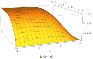
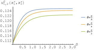
Figure 1: The payoff at quantum Nasha equlibrium described by eq. (35) as a function of the phase parameter $\theta$ and the squeezing parameter $\beta$; $k=1$.

The payoff function described by eq. (33) depends on four parameter. The graphs of this function for selected values of phase parameters are given on Figure 2.

As can be seen from Fig. 1 for the $\theta\in(0,\frac{\pi}{2})$ the players cannot reach the maximum value of payoff in the model depending on only one squeezing parameter $\beta$. In contrast, when the entanglement operator depends on two squeezing parameters, the payoff function $\tilde{u}_{1,2}^{Q}(\tilde{x}_{1}^{*},\tilde{x}_{2}^{*})$ can reach its maximum value even if $\theta,\phi\neq 0$, see Figure 2 and 3.

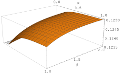
(a) $\phi=\theta=\frac{\pi}{4}$

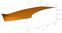
(b) $\phi=\frac{\pi}{3}$, $\theta=\frac{3\pi}{4}$

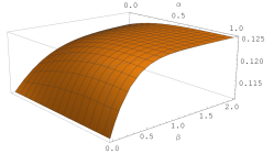
(c) $\phi=\frac{3\pi}{4}$, $\theta=\frac{\pi}{3}$

Figure 2: The payoffs at quantum Nasha equlibrium described by eq. (33) as a function of the squeezing parameters $\alpha$, $\beta$; $k=1$.

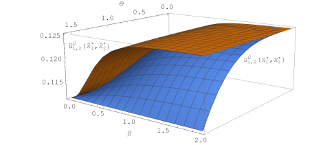
Figure 3: The payoffs at quantum Nasha equlibrium described by eqs. (35) (the blue surface) and (33) (the orange surface) for $\phi=\theta$ and $\alpha=\beta$; $k=1$.

V Degree of entanglement versus payoff of the quantum game

Both for the games with discrete as well as continuous sets of strategies, the advantage of quantum games as compared to their classical counterparts is due to the entanglement of the initial state of the game. The largest payoff values in Nash equilibrium are obtained with maximally entangled states. When the entanglement parameter goes to zero the quantum game coincides with its classical counterpart.
Let us compare the degrees of entanglement of the games based on $\hat{J}(\xi)$ and $\hat{J}_{1}(\delta,\xi)$ (defined by eqs. (34) and (15)) and their payoff values in Nash equilibrium. To determine the degree of entanglement of a game, we must use some measure of entanglement. For Gaussian states, which we are dealing with, many measures of entanglement can be found in the literature [47],[48].

One of the simplest measures is the entropy of entanglement which, for a pure state, can be expressed in terms of the covariance matrix. For a bipartite Gaussian pure state, entanglement entropy is of the form [49]

$$S=\sum_{i=1}^{n_{sub}}\left[\left(\mu_{i}+\frac{1}{2}\right)\log_{2}\left(\mu_{i}+\frac{1}{2}\right)-\left(\mu_{i}-\frac{1}{2}\right)\log_{2}\left(\mu_{i}-\frac{1}{2}\right)\right]$$ (37)

where $\mu_{i}$ are the symplectic eigenvalues of the correlation matrix $\sigma$ of any of the subsystems. It remains to explain what symplectic eigenvalues are.

Let us define the column vector

$$\hat{r}=\left(\begin{array}[]{c}\hat{X}_{1}\\ \hat{P}_{1}\\ \hat{X}_{2}\\ \hat{P}_{2}\end{array}\right)$$ (38)

where $\hat{X}_{k}$, $\hat{P}_{k}$ , $k=1,2$, are position- and momentum operators with the canonical commutator $[\hat{X}_{k},\hat{P}_{l}]=i\delta_{kl}$. The vector $\hat{r}$ obeys the following commutation relations

$$[\hat{r}_{k},\hat{r}_{l}]=i\Omega_{kl}$$ (39)

where

$$\Omega=\bigoplus\limits_{k=1}^{2n}\Bigg{(}\begin{matrix}0&1\\ -1&0\end{matrix}\Bigg{)}=\mathbbm{1}_{n}\otimes\Bigg{(}\begin{matrix}0&1\\ -1&0\end{matrix}\Bigg{)}$$ (40)

is a symplectic matrix, $\mathbbm{1}_{n}$ being the $n\times n$ identity matrix. The inverse of the matrix $\Omega$ is

$$\Omega^{-1}=\Omega^{T}=-\Omega.$$ (41)

For Gaussian states we can define Gaussian unitary operation as a transformation that maps Gaussian state onto a Gaussian state. To such a transformation we can assign a unique symplectic transformation $S\in Sp(2n,\mathbbm{R})$ that preserves the commutation relations

$$i\Omega=[\hat{r}^{\prime}_{k},\hat{r}^{\prime}_{l}]=S[\hat{r}_{k},\hat{r}_{l}]S^{T},$$ (42)

thus $\Omega=S\Omega S^{T}$.
The covariance matrix of n-mode system defined by

$$\sigma_{kl}=\frac{1}{2}\left<\{\hat{r}_{k},\hat{r}_{l}\}\right>-\left<\hat{r}_{k}\right>\left<\hat{r}_{l}\right>,$$ (43)

where $\{\cdot,\cdot\}$ denotes an anticommutator, transforms under the action of a symplectic transformation as follows

$$\sigma^{\prime}=S\sigma S^{T}.$$ (44)

According to Williamson’s theorem [50], any real symmetric positive-define $2n\times 2n$ matrix can be diagonalized by an appropriate symplectic transformation $S_{w}\in Sp(2n,\mathbbm{R})$:

$$S_{w}\sigma S_{w}^{T}=\sigma_{w}$$ (45)

where

$$\sigma_{w}=diag(\mu_{1},\mu_{2},\ldots,\mu_{n},\mu_{1},\mu_{2},\ldots,\mu_{n}).$$ (46)

All the $\mu_{i}$ are real and the $n$ distinct eigenvalues of $\sigma_{w}$ are the symplectic eigenvalues of the covariance matrix $\sigma$.

In order to find the values $\mu_{i}$, let us consider, for any covariance matrix $\sigma$, a new matrix $K$ such that

$$\sigma=-K\Omega.$$ (47)

Multiplying both sides of the equation (47) from the right by $\Omega^{-1}$ and using the equation (41) we get

$$K=\sigma\Omega.$$ (48)

If two covariance matrices $\sigma$, $\sigma^{\prime}$ are related by a symplectic transformation then the corresponding $K$ and $K^{\prime}$ matrices are related by similarity transformation

$$K^{\prime}=\sigma^{\prime}\Omega=S\sigma S^{T}\Omega=S\sigma\Omega S^{-1}=SKS^{-1}$$ (49)

which means that the matrices K and K’ have the same eigenvalues. We can check that the eigenvalues of $K^{\prime}=\sigma_{w}\Omega$ are equal to $\{\pm i\mu_{i}\}$. Thus, in order to find the symplectic eigenvalues of the covariance matrix $\sigma$, it is enough to determine the eigenvalues of the matrix $K=\sigma\Omega$.

Now we can find how the entanglement entropy of initial state depends on the entanglement operator.

1. The degree of entanglement of the initial state $\left|\Psi_{0}\right>=\hat{J}(\xi)\left|00\right>$
   First, we determine the covariance matrix of one of the subsystems (the covariance matrices for both subsystems are the same). According to the eq. (43) it reads

   $$\sigma_{1}=\begin{pmatrix}\frac{1}{2}\cosh(2\beta)&0\\ 0&\frac{1}{2}\cosh(2\beta)\end{pmatrix}$$ (50)

   from which we can directly determine the symplectic eigenvalues. Thus, the entanglement entropy, eq. (37) has form

   $$S_{1}=\frac{\cosh(2\beta)\ln(\coth\beta)+\ln(\cosh\beta\sinh\beta)}{\ln 2}.$$ (51)

   As we can see from Figure 4 the values of the entanglement measure $S_{1}$ increase with the $\beta$.

   

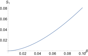
   Figure 4: The entanglement entropy of state $\left|\Psi_{0}\right>=\hat{J}(\xi)\left|00\right>$

2. The degree of entanglement of the initial state $\big{|}\tilde{\Psi}_{0}\big{>}=\hat{J_{1}}(\delta,\xi)\left|00\right>$
   In the case of an initial state based on the entanglement operator $\hat{J}_{1}(\delta,\xi)$, the covariance matrix $\tilde{\sigma}_{1}$ of the first subsystem has a more complicated form (the covariance matrix of the second subsystem is equal the covariance matrix of the first one). Its matrix elements are

   $$\begin{split}&\tilde{\sigma}_{11}=\frac{1}{8}(2(\cosh(2a)+\cosh(2b))-(\frac{1}{ad}+ad)\sinh(2a)-(\frac{1}{bf}+bf)\sinh(2b)),\\ &\tilde{\sigma}_{12}=\tilde{\sigma}_{21}=\frac{1}{8}((ad-\frac{1}{ad})\sinh(2a)+(bf-\frac{1}{bf})\sinh(2b)),\\ &\tilde{\sigma}_{22}=\frac{1}{8}(2\cosh(2a)+2\cosh(2b)+(ad+\frac{1}{ad})\sinh(2a)+(bf+\frac{1}{bf})\sinh(2b))\end{split}$$ (52)

   where $a,\,b,\,d,\,f$ are defined by eq. (27). According to the procedure described above, we multiply the covariance matrix of the subsystem $\tilde{\sigma}_{1}$ by the symplectic matrix $\Omega$, defined by eq. (41), and then we look for the eigenvalues of the resulting matrix. In this way, we obtain the following symplectic eigenvalues

   $$\begin{split}\tilde{\mu}_{1}&=\tilde{\mu}_{2}=\frac{1}{4}\sqrt{2+2\cosh(2a)\cosh(2b)-(\frac{ad}{bf}+\frac{bf}{ad})\sinh(2a)\sinh(2b)}\\ &=\frac{1}{4}\bigg{(}2+2\cosh(2\sqrt{4\alpha^{2}+\beta^{2}-4\alpha\beta\cos(\theta-\phi)})\cosh(2\sqrt{4\alpha^{2}+\beta^{2}+4\alpha\beta\cos(\theta-\phi)})\\ &-\frac{2(4\alpha^{2}-\beta^{2})\sinh(2\sqrt{4\alpha^{2}+\beta^{2}-4\alpha\beta\cos(\theta-\phi)})\sinh(2\sqrt{4\alpha^{2}+\beta^{2}+4\alpha\beta\cos(\theta-\phi)})}{\sqrt{16\alpha^{4}+\beta^{4}-8\alpha^{2}\beta^{2}\cos(2\theta-2\phi)}}\bigg{)}^{1/2}\end{split}$$ (53)

   and the entanglement entropy

   $$\tilde{S}_{1}=\frac{1}{\ln 4}\left((1+2\tilde{\mu}_{1})\ln\bigg{(}\tilde{\mu}_{1}+\frac{1}{2}\bigg{)}+(1-2\tilde{\mu}_{1})\ln\bigg{(}\tilde{\mu}_{1}-\frac{1}{2}\bigg{)}\right).$$ (54)

   The eigenvalues (53) are periodic functions of $\theta$ and $\phi$ with period $\pi$ and depend on the difference of phase parameters. Thus the entropy function $\tilde{S}_{1}$ actually depends on three parameters $\alpha,\beta>0$, and $0\leq\theta-\phi<\pi$.

   Let us see how the function $\tilde{S}_{1}$ behaves in a few special cases:

   • for $\phi=\theta$ and $\alpha,\beta>0$ we obtain $\tilde{S}_{1}=S_{1}$, where $S_{1}$ is described by eq. (51);

   • for $\alpha=\beta$ and $0\leq\theta-\phi<\pi$ the symplectic eigenvalue and the entanglement entropy increase with the entanglement parameter $\beta$; the fastest grow corresponds to $\theta-\phi=\frac{\pi}{2}$, see Firgure 5.

     

     

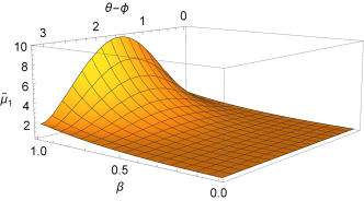
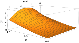
     Figure 5: The symplectic eigenvalue $\tilde{\mu}_{1}$ (a) of the covariance matrix of subsystem and the entanglement entropy $\tilde{S}_{1}$ (b) for $\alpha=\beta$ and $0\leq\theta-\phi<\pi$.

   • for $\alpha,\beta>0$ and $\theta-\phi=\{\frac{\pi}{6},\frac{\pi}{4},\frac{\pi}{2}\}$, the higher the value of $\alpha$ and $\beta$, the higher the entanglement entropy value, cf. Figure 6.

     

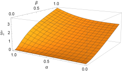
     (a) $\theta-\phi=\frac{\pi}{6}$

     

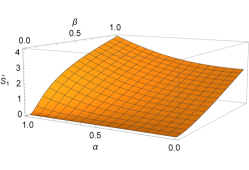
     (b) $\theta-\phi=\frac{\pi}{4}$

     

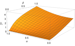
     (c) $\theta-\phi=\frac{\pi}{3}$

     Figure 6: The entanglement entropy $\tilde{S}_{1}$ for determined value of $\theta-\phi$.

Now, let us try to analyze how the payoffs of the players in the Cournot model depend on the degree of entanglement of initial state of the game.

Case I.

Let $\phi=\theta$; then, according to the measures $S_{1}$ and $\tilde{S}_{1}$, the entanglement degrees of the initial states $\left|\Psi_{0}\right>$, $|\tilde{\Psi}_{0}\big{>}$ are the same, the entanglement measure depending on only one squeezing parameter $\beta$. However, the payoff functions based on these states are different and depend on entanglement and phase parameters. Assuming specific values of the phase parameters (see Figure 7), we see that the payoff $\tilde{u}_{1}^{Q}(\tilde{x}_{1}^{*},\tilde{x}_{2}^{*})$ (eq. (33)) is always higher than the payoff $u_{1}^{Q}(x_{1}^{*},x_{2}^{*})$ (eq. (35)).

In addition, it can be seen that the difference between the payoffs in the games under consideration depend on the value of the parameters $\phi,\,\theta$. The payoff $u_{1}^{Q}(x_{1}^{*},x_{2}^{*})$ is

• an increasing function of the parameter $\beta$ for $\theta\in\big{[}0,\frac{\pi}{2}\big{)}\cup\big{(}\frac{3\pi}{2},2\pi\big{]}$,

• a constant function for $\theta=\{\frac{\pi}{2},\frac{3\pi}{2}\}$,

• a decreasing function as $\beta$ increases for $\theta\in\big{(}\frac{\pi}{2},\frac{3\pi}{2}\big{)}$.

The effect of the parameter $\theta$ on $\tilde{u}_{1}^{Q}(\tilde{x}_{1}^{*},\tilde{x}_{2}^{*})$ can also be studied. For small values of $\alpha$, the function $\tilde{u}_{1}^{Q}(\tilde{x}_{1}^{*},\tilde{x}_{2}^{*})$ behaves similarly to $u_{1}^{Q}(x_{1}^{*},x_{2}^{*})$, i.e. for $\theta\in\big{(}\frac{\pi}{2},\frac{3\pi}{2}\big{)}$ the payoff decreases as $\beta$ increases. However, as the value of the parameter $\alpha$ increases, the properties of the function $\tilde{u}_{1}^{Q}(\tilde{x}_{1}^{*},\tilde{x}_{2}^{*})$ change and it transforms into a function which increases with the parameter $\beta$ (see Fig. 7(e) and 7(f)).

The dependence of payoff functions on the phase parameters for selected values of the entanglement parameters is illustrated on Figure 8. We see that the higher the value of the parameter $\alpha$, the greater the difference between the payoffs $\tilde{u}_{1}^{Q}(\tilde{x}_{1}^{*},\tilde{x}_{2}^{*})$ and $u_{1}^{Q}(x_{1}^{*},x_{2}^{*})$.

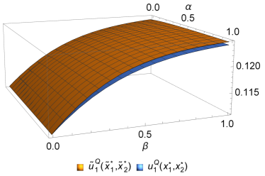
(a) $\phi=\theta=\frac{\pi}{6}$

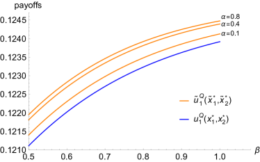
(b) the payoffs from subpoint (a) for selected $\alpha$

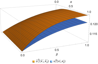
(c) $\phi=\theta=\frac{\pi}{3}$

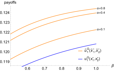
(d) the payoffs from subpoint (c) for selected $\alpha$

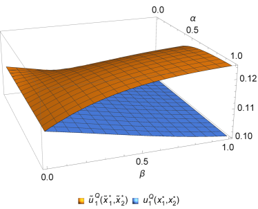
(e) $\phi=\theta=\frac{7\pi}{5}$

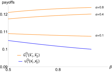
(f) the payoffs from subpoint (e) for selected $\alpha$

Figure 7: The payoffs in Nash equlibrium of games based on the entangled operators $\hat{J}(\xi)$ and $\hat{J}_{1}(\delta,\xi)$ for $\theta=\phi$, $k=1$.

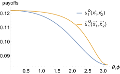
(a) $\alpha=0.3$, $\beta=0.5$

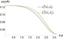
(b) $\alpha=0.1$, $\beta=1$

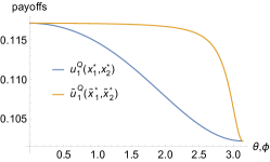
(c) $\alpha=1$, $\beta=0.2$

Figure 8: The payoffs $\tilde{u}_{1}^{Q}(\tilde{x}_{1}^{*},\tilde{x}_{2}^{*})$ and $u_{1}^{Q}(x_{1}^{*},x_{2}^{*})$ for selected values of parameters $\alpha$, $\beta$ and $\theta=\phi$.

.

Case II.

Now, let us see how the payoff functions behave when $\alpha=\beta$ and $\theta,\phi\in\big{[}0,2\pi)$. In this case the entanglement entropy $S_{1}$ has different form than $\tilde{S}_{1}$. The payoff function ${u}_{1}^{Q}({x}_{1}^{*},{x}_{2}^{*})$ depends on two variables, while $\tilde{u}_{1}(\tilde{x}_{1}^{*},\tilde{x}_{2}^{*})$ depends on three. Therefore, let us analyze some cases with specific values of one of the phase parameters.

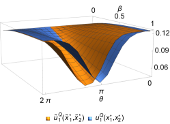
(a) $\phi=\frac{\pi}{3}$,

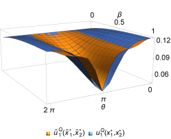
(b) $\phi=\pi$

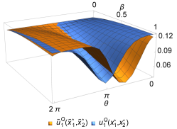
(c) $\phi=\frac{7\pi}{5}$

Figure 9: The payoffs $\tilde{u}_{1}^{Q}(\tilde{x}_{1}^{*},\tilde{x}_{2}^{*})$ and $u_{1}^{Q}(x_{1}^{*},x_{2}^{*})$ for $\alpha=\beta$ and selected values of parameter $\phi$.

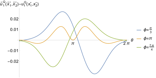
Figure 10: The difference between payoffs $\tilde{u}_{1}^{Q}(\tilde{x}_{1}^{*},\tilde{x}_{2}^{*})$ and $u_{1}^{Q}(x_{1}^{*},x_{2}^{*})$ for selected values of $\phi$ and $\alpha=\beta=0.8$.

First, let us analyze the properties of $\tilde{u}_{1}(\tilde{x}_{1}^{*},\tilde{x}_{2}^{*})$ for specific values of the parameter $\phi$. Unlike the case I, the values of $\tilde{u}_{1}(\tilde{x}_{1}^{*},\tilde{x}_{2}^{*})$ are not always higher than the values of ${u}_{1}^{Q}({x}_{1}^{*},{x}_{2}^{*})$ (Fig. 9). By analyzing the difference between the payoffs obtained in games based on entanglement operator $\hat{J}(\xi)$ and $\hat{J}_{1}(\delta,\xi)$, it can be seen that the phase parameters can be chosen in such a way that ${u}_{1}^{Q}({x}_{1}^{*},{x}_{2}^{*})$ gives significantly more favorable results as compared to $\tilde{u}_{1}(\tilde{x}_{1}^{*},\tilde{x}_{2}^{*})$, see Fig. 10. Fixing some value of the parameter $\beta$, we can numerically find the values of the phase parameters for which the difference $\tilde{u}_{1}^{Q}(\tilde{x}_{1}^{*},\tilde{x}_{2}^{*})-u_{1}^{Q}(x_{1}^{*},x_{2}^{*})$ reaches a maximum or minimum; the results are shown in Table 1. As one can see, we can choose a set of parameter values for which the game based on $\hat{J}(\xi)$ gives more favorable results.

If we compare the degree of entanglement of the two games, we find that the entanglement entropy $\tilde{S}_{1}$ is always greater than or equal to $S_{1}$ (Fig. 11). Even in the cases when $u_{1}^{Q}(x_{1}^{*},x_{2}^{*})$ payoffs are higher than $\tilde{u}_{1}^{Q}(\tilde{x}_{1}^{*},\tilde{x}_{2}^{*})$, the selected measure of entanglement indicates a higher degree of entanglement for the model based on $\hat{J}_{1}(\delta,\xi)$ as compared with that based on $\hat{J}(\xi)$ (Table 1).

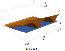
(a) $\phi=\frac{\pi}{3}$, $\alpha=\beta$

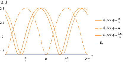
(b) $\alpha=\beta=0.7$

Figure 11: The entanglement entropies $\tilde{S}_{1}$ and $S_{1}$ for selected values of phase parameter $\phi$.

		fixed $\alpha$ and $\beta$, with $\alpha=\beta$
		0.2	0.5	1	5
$\max(\tilde{u}_{1}^{Q}(\tilde{x}_{1}^{*},\tilde{x}_{2}^{*})-u_{1}^{Q}(x_{1}^{*},x_{2}^{*}))$		0.0030	0.0195	0.0648	0.1250
estimated parameters $\Bigg{\{}$	$\theta$	2.0525	2.4987	2.8611	3.1416
	$\phi$	1.8324	2.1704	2.5492	3.3488
entropy for the estimated parameter $\theta$ and $\phi$ $\Bigg{\{}$	$\tilde{S}_{1}$	0.2491	1.0499	3.1337	24.2017
	$S_{1}$	0.2471	0.9514	2.3369	13.8696
$\min(\tilde{u}_{1}^{Q}(\tilde{x}_{1}^{*},\tilde{x}_{2}^{*})-u_{1}^{Q}(x_{1}^{*},x_{2}^{*}))$		-0.0003	-0.0235	-0.0832	-0.1250
estimated parameters $\Bigg{\{}$	$\theta$	6.2832	1.7687	1.5048	0.1151
	$\phi$	4.5132	4.0706	3.7487	3.1994
entropy for the estimated parameter $\theta$ and $\phi$ $\Bigg{\{}$	$\tilde{S}_{1}$	0.2860	1.3707	4.3336	23.5971
	$S_{1}$	0.2471	0.9514	2.3369	13.8696

Table 1: Values of phase parameters estimated numerically, for which the difference between payoffs at fixed $\alpha,\beta$ ($\alpha=\beta$) values is the largest or smallest.

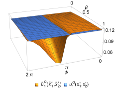
(a) $\theta=\frac{\pi}{3}$,

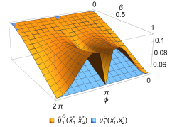
(b) $\theta=\pi$

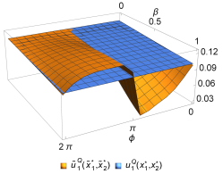
(c) $\theta=\frac{7\pi}{5}$

Figure 12: The payoffs $\tilde{u}_{1}^{Q}(\tilde{x}_{1}^{*},\tilde{x}_{2}^{*})$ and $u_{1}^{Q}(x_{1}^{*},x_{2}^{*})$ for $\alpha=\beta$ and selected values of parameter $\theta$.

Let us now analyze the properties of the $\tilde{u}_{1}^{Q}(\tilde{x}_{1}^{*},\tilde{x}_{2}^{*})$ and $u_{1}^{Q}(x_{1}^{*},x_{2}^{*})$, choosing the specific values of the parameter $\theta$. For $\theta=\pi$, we always get higher payoffs for the game based on $\hat{J}_{1}(\delta,\xi)$ than for that based on $\hat{J}(\xi)$ (Figure 12). Note that the payoff $u_{1}^{Q}(x_{1}^{*},x_{2}^{*})$ does not depend on the $\phi$ parameter and is an increasing function of $\beta$ for $\theta\in[0,\frac{\pi}{2})\cup(\frac{3\pi}{2},2\pi)$ and a decreasing function for $\theta\in(\frac{\pi}{2},\frac{3\pi}{2})$. It can be deduced from Figure 12 and 13 that both phase parameters have a strong influence on the variation of the function $\tilde{u}_{1}^{Q}(\tilde{x}_{1}^{*},\tilde{x}_{2}^{*})$. The entanglement entropy $\tilde{S}_{1}$ depends on the phase parameters through $\cos(\theta-\phi)$, so the graph of the function $\tilde{S}_{1}(\phi)$ at fixed $\theta$ and $\beta$ is the same as graph of $\tilde{S}_{1}(\theta)$ on Fig. 11(b).

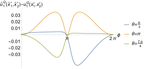
Figure 13: The difference between payoffs $\tilde{u}_{1}^{Q}(\tilde{x}_{1}^{*},\tilde{x}_{2}^{*})$ and $u_{1}^{Q}(x_{1}^{*},x_{2}^{*})$ for selected values of $\theta$ and $\alpha=\beta=0.8$.

Case III.

Consider the case where $\theta-\phi=const.$ and $\alpha,\beta>0$, which is interesting because the entanglement entropy $\tilde{S}_{1}$ depends only on the difference of phase parameters. Let us choose the range of the values of the parameter $\theta$ from 0 to $\frac{\pi}{2}$, for which the function $u_{1}^{Q}(x_{1}^{*},x_{2}^{*})$ increases with the increasing squeezing parameter $\beta$. When $\theta\in(0,\frac{\pi}{2})$, $\tilde{u}_{1}^{Q}(\tilde{x}_{1}^{*},\tilde{x}_{2}^{*})$ is also an increasing function of both squeezing parameters $\alpha$ and $\beta$. As shown on Figures 14(c), 14(f), 14(i) the higher the values of the difference of phase parameters, the higher values reaches the measure of entanglement $\tilde{S}_{1}$ as the parameters $\alpha$ and $\beta$ increase; in all cases $\tilde{S}_{1}\geq S_{1}$. Comparing Figure 14(a) with 14(b) (14(d) with 14(e), 14(g) with 14(h)), we see that the difference between the payoffs $\tilde{u}_{1}^{Q}(\tilde{x}_{1}^{*},\tilde{x}_{2}^{*})$ and $u_{1}^{Q}(x_{1}^{*},x_{2}^{*})$ increases as the parameter $\theta$ increases. The reason for this is that for $\theta\rightarrow\frac{\pi}{2}$ values of $u_{1}^{Q}(x_{1}^{*},x_{2}^{*})$ grow slower and slower as the functions of $\beta$, while for the $\tilde{u}_{1}^{Q}(\tilde{x}_{1}^{*},\tilde{x}_{2}^{*})$ the additional squeezing parameter $\alpha$ allows for the maximum value of the payoff to be reached every time.

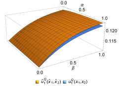
(a) $\theta-\phi=\frac{\pi}{6}$, $\phi=0.3*\frac{\pi}{3}$

(b) $\theta-\phi=\frac{\pi}{6}$, $\phi=0.8*\frac{\pi}{3}$

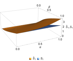
(c) $\theta-\phi=\frac{\pi}{6}$

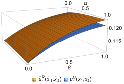
(d) $\theta-\phi=\frac{\pi}{4}$, $\phi=0.3*\frac{\pi}{4}$

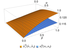
(e) $\theta-\phi=\frac{\pi}{4}$, $\phi=0.8*\frac{\pi}{4}$

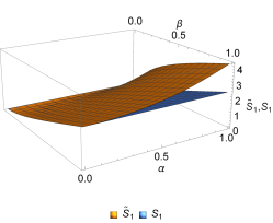
(f) $\theta-\phi=\frac{\pi}{4}$

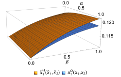
(g) $\theta-\phi=\frac{\pi}{3}$, $\phi=0.3*\frac{\pi}{6}$

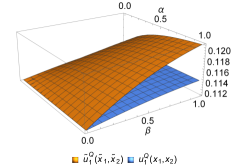
(h) $\theta-\phi=\frac{\pi}{3}$, $\phi=0.3*\frac{\pi}{6}$

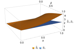
(i) $\theta-\phi=\frac{\pi}{3}$

Figure 14: The payoffs in Nash equlibrium of games based on the entangled operators $\hat{J}(\xi)$, $\hat{J}_{1}(\delta,\xi)$ and corresponding entanglement entropies for fixed values of $\theta$ and $\phi$ that satisfy the condition $\theta-\phi=\frac{\pi}{6},\frac{\pi}{4},\frac{\pi}{3}$.

VI Conclusions

The quantization scheme of games containing a continuous set of strategies proposed by Li et al. made it possible to analyze the quantum counterpart of the duopoly models known in economics. The best known yet very simple model is Cournot’s duopoly, for which the corresponding quantum model leads to higher payoffs as compared to the classical one. This effect is due to the entanglement of the initial state of the game; Li et al. showed that the higher the value of the squeezing parameter, the higher the payoffs of players in Nash equilibrium; the initial state of the game they considered depended on only one parameter - the squeezing parameter.

Due to the key role of the game degree of entanglement on its outcome, we decided to consider the quantum Cournot model based on the most general entanglement operator $\hat{J}_{1}(\delta,\xi,)$ satisfying the assumptions concerning the symmetry with respect to the exchange of players and full representativeness of the classical game by its quantum counterpart and depending on two squeezing and two phase parameters.

The main conclusion of the analysis is the observation that the relationship between the degree of entanglement of the game initial state and the payoff values in Nash equilibrium is ambiguous. For fixed phase values, the entanglement entropy of the initial state increases with the entanglement parameters, but the phase parameters can be chosen so that a game based on the initial state $\hat{J}_{1}(\delta,\xi,)|00\big{>}$ gives lower payoffs than a game depending on a single entanglement parameter (see Table 1).

Phase parameters also have great impact on the outcome of the game. In the case of the game based on the entanglement operator $\hat{J}(\xi)$, the maximum possible outcome of the game with $\beta\rightarrow\infty$ becomes lower and lower as the phase parameter $\theta$ goes to $\frac{\pi}{2}$. When the game depends on two squeezing parameters, it is possible to reach the maximum payoff in Nash equilibrium when $\alpha\rightarrow\infty$ and the phase parameters satisfy the condition $\theta-\phi=const.$ (Fig. 14). As shown in Section IV, it is not possible to achieve an arbitrarily large payoff in Nash equilibrium when $\alpha,\beta\rightarrow\infty$. The maximum payoff a player can receive in Nash equilibrium of the model under consideration is $\frac{k^{2}}{8}$.

Acknowledgement

I am grateful to Prof. Piotr Kosiński and Prof. Krzysztof Andrzejewski for helpful discussion and useful remarks.

Appendix A

In paper [46], the authors considered an entanglement operator of the game of the form

$$\hat{J}(\gamma_{1},\gamma_{2},\gamma_{12})=e^{\gamma_{12}(a_{1}a_{2}-a_{1}^{\dagger}a_{2}^{\dagger})}e^{\gamma_{1}(a_{1}^{2}-a_{1}^{\dagger\,2})/2}e^{\gamma_{2}(a_{2}^{2}-a_{2}^{\dagger\,2})/2}$$ (55)

where $\gamma_{1},\,\gamma_{2},\,\gamma_{12}\in R$ and $\gamma_{12}\geq 0$. This operator satisfies the condition that the classical game is to be fully represented by its quantum counterpart, but does not satisfy the symmetry condition with respect to the exchange of players. The entanglement operator defined by eq. (15) satisfies both of these conditions.

Using the position $\hat{X_{j}}=(a_{j}^{\dagger}+a_{j})/\sqrt{2}$ and momentum $\hat{P_{j}}=i(a_{j}^{\dagger}-a_{j})/\sqrt{2}$ operators the entanglement operator (55) can be rewritten in the following form

$$\hat{J}(\gamma_{1},\gamma_{2},\gamma_{12})=e^{i\gamma_{12}(\hat{X}_{1}\hat{P}_{2}+\hat{X}_{2}\hat{P}_{1})}e^{i\gamma_{1}(\hat{X}_{1}\hat{P}_{1}+\hat{P}_{1}\hat{X}_{1})/2}e^{i\gamma_{2}(\hat{X}_{2}\hat{P}_{2}+\hat{P}_{2}\hat{X}_{2})/2}.$$ (56)

and is equivalent to the operator

$$\hat{J}(\gamma_{1},\gamma_{2},\gamma_{12})=e^{iA_{1}\hat{X}_{1}\hat{P}_{2}+iA_{2}\hat{X}_{2}\hat{P}_{1}+iB_{1}(\hat{X}_{1}\hat{P}_{1}+\hat{P}_{1}\hat{X}_{1})+iB_{2}(\hat{X}_{2}\hat{P}_{2}+\hat{P}_{2}\hat{X}_{2})+iC_{1}}$$ (57)

where

$$\begin{split}A_{1}&=\frac{r\sinh\gamma_{12}}{\sinh r}e^{-\frac{\gamma_{1}-\gamma_{2}}{2}},\\ A_{2}&=\frac{r\sinh\gamma_{12}}{\sinh r}e^{\frac{\gamma_{1}-\gamma_{2}}{2}},\\ B_{1}&=\frac{1}{4}\left(\gamma_{1}+\gamma_{2}+\frac{2r\cosh\gamma_{12}}{\sinh r}\sinh\left(\frac{\gamma_{1}-\gamma_{2}}{2}\right)\right),\\ B_{2}&=\frac{1}{4}\left(\gamma_{1}+\gamma_{2}-\frac{2r\cosh\gamma_{12}}{\sinh r}\sinh\left(\frac{\gamma_{1}-\gamma_{2}}{2}\right)\right),\\ C_{1}&-\text{any real value},\\ r&=\operatorname{arccosh}\left(\cosh\left(\frac{\gamma_{1}-\gamma_{2}}{2}\right)\cosh\gamma_{12}\right).\end{split}$$

The $iC_{1}$ factor contained in the operator $\hat{J}(\gamma_{1},\gamma_{2},\gamma_{12})$ (57) can be ignored because it has no effect on the final state of the game.

For $\gamma_{1}=\gamma_{2}$, the operator $\hat{J}(\gamma_{1},\gamma_{2},\gamma_{12})$ becomes symmetric due to the exchange of players and simplifies to a form

$$\hat{J}(\gamma_{1},\gamma_{1},\gamma_{12})=e^{\gamma_{12}(a_{1}a_{2}-a_{1}^{\dagger}a_{2}^{\dagger})-\frac{\gamma_{1}}{2}(a_{1}^{\dagger\,2}+a_{2}^{\dagger\,2}-a_{1}^{2}-a_{2}^{2})}$$ (58)

which is a special case of the operator $\hat{J}_{1}(\delta,\xi)$ defined by eq. (15) when $\theta=\phi=0$, $\beta=\gamma_{12}$ and $\delta=\frac{\gamma_{1}}{2}$.

Appendix B

To find the expansion of $e^{M}$ where

$$M=\left(\begin{array}[]{cccc}0&0&2\delta&\xi\\ 0&0&\xi&2\delta\\ 2\delta^{*}&\xi^{*}&0&0\\ \xi^{*}&2\delta^{*}&0&0\end{array}\right)=\left(\begin{array}[]{cccc}0&0&2\alpha e^{i\phi}&\beta e^{i\theta}\\ 0&0&\beta e^{i\theta}&2\alpha e^{i\phi}\\ 2\alpha e^{-i\phi}&\beta e^{-i\theta}&0&0\\ \beta e^{-i\theta}&2\alpha e^{-i\phi}&0&0\end{array}\right)$$ (59)

one can diagonalize the matrix M by transformation

$$M=SM_{diag}S^{-1}$$ (60)

and then use the formula

$$e^{M}=Se^{M_{diag}}S^{-1}.$$ (61)

$M_{diag}$ is a diagonal matrix with elements on the main diagonal which are the eigenvalues of the matrix $M$ and the corresponding eigenvectors of $M$ are the consecutive columns of the matrix $S$. Finding the eigenvalues and eigenvectors of the matrix M, one can write

$$M_{diag}=\left(\begin{array}[]{cccc}-a&0&0&0\\ 0&a&0&0\\ 0&0&-b&0\\ 0&0&0&b\end{array}\right),\quad S=\left(\begin{array}[]{cccc}\frac{e^{i(\theta+\phi)}a}{2e^{i\theta}\alpha-e^{i\phi}\beta}&-\frac{e^{i(\theta+\phi)}a}{2e^{i\theta}\alpha-e^{i\phi}\beta}&-\frac{e^{i(\theta+\phi)}b}{2e^{i\theta}\alpha+e^{i\phi}\beta}&\frac{e^{i(\theta+\phi)}b}{2e^{i\theta}\alpha+e^{i\phi}\beta}\\ -\frac{e^{i(\theta+\phi)}a}{2e^{i\theta}\alpha-e^{i\phi}\beta}&\frac{e^{i(\theta+\phi)}a}{2e^{i\theta}\alpha-e^{i\phi}\beta}&-\frac{e^{i(\theta+\phi)}b}{2e^{i\theta}\alpha+e^{i\phi}\beta}&\frac{e^{i(\theta+\phi)}b}{2e^{i\theta}\alpha+e^{i\phi}\beta}\\ -1&-1&1&1\\ 1&1&1&1\end{array}\right)$$ (62)

where $a=\sqrt{4\alpha^{2}+\beta^{2}-4\alpha\beta\cos(\theta-\phi)}$, $b=\sqrt{4\alpha^{2}+\beta^{2}+4\alpha\beta\cos(\theta-\phi)}$.

It is not difficult to find $e^{M_{diag}}$

$$e^{M_{diag}}=\left(\begin{array}[]{cccc}\cosh a-\sinh a&0&0&0\\ 0&\cosh a+\sinh a&0&0\\ 0&0&\cosh b-\sinh b&0\\ 0&0&0&\cosh b+\sinh b\end{array}\right).$$ (63)

Using eq. (61) one can find $e^{M}$; its final form is described by the eq. (26).

Appendix C

The quantum payoff functions $\tilde{u}_{1,2}^{Q}(\tilde{x}_{1},\tilde{x}_{2})$ are obtained by substituting $\tilde{q}_{1}$ and $\tilde{q}_{2}$, described by the equation (29), into the payoff functions defined by the equation (4). Their explicit forms are

$$\begin{split}\tilde{u}_{1}^{Q}(\tilde{x}_{1},\tilde{x}_{2})=&\frac{1}{8}\left(2k-\left(2\cosh b+\left(\frac{1}{bf}+bf\right)\sinh b\right)(x_{1}+x_{2})\right)\\ &\cdot\left(\left(2\cosh a+\left(\frac{1}{ad}+ad\right)\sinh a\right)(x_{1}-x_{2})+\left(2\cosh b+\left(\frac{1}{bf}+bf\right)\sinh b\right)(x_{1}+x_{2})\right),\\ \tilde{u}_{2}^{Q}(\tilde{x}_{1},\tilde{x}_{2})=&\frac{1}{8}\left(2k-\left(2\cosh b+\left(\frac{1}{bf}+bf\right)\sinh b\right)(x_{1}+x_{2})\right)\\ &\cdot\left(\left(2\cosh a+\left(\frac{1}{ad}+ad\right)\sinh a\right)(x_{2}-x_{1})+\left(2\cosh b+\left(\frac{1}{bf}+bf\right)\sinh b\right)(x_{1}+x_{2})\right).\end{split}$$ (64)

Using eq. (27) we obtain the following payoff functions

$$\begin{split}&\tilde{u}_{i}^{Q}(\tilde{x}_{1},\tilde{x}_{2})=\\ &=\frac{1}{2}\Bigg{[}k-\Bigg{(}\cosh\sqrt{4\alpha^{2}+\beta^{2}+4\alpha\beta\cos(\theta-\phi)}+\frac{(\beta\cos\theta+2\alpha\cos\phi)\sinh\sqrt{4\alpha^{2}+\beta^{2}+4\alpha\beta\cos(\theta-\phi)}}{\sqrt{4\alpha^{2}+\beta^{2}+4\alpha\beta\cos(\theta-\phi)}}\Bigg{)}(x_{i}+x_{j})\Bigg{]}\\ &\cdot\Bigg{[}\cosh\sqrt{4\alpha^{2}+\beta^{2}-4\alpha\beta\cos(\theta-\phi)}+\frac{(-\beta\cos\theta+2\alpha\cos\phi)\sinh\sqrt{4\alpha^{2}+\beta^{2}-4\alpha\beta\cos(\theta-\phi)}}{2\sqrt{4\alpha^{2}+\beta^{2}-4\alpha\beta\cos(\theta-\phi)}}\Bigg{)}(x_{i}-x_{j})\\ &+\Bigg{(}\cosh\sqrt{4\alpha^{2}+\beta^{2}+4\alpha\beta\cos(\theta-\phi)}+\frac{(\beta\cos\theta+2\alpha\cos\phi)\sinh\sqrt{4\alpha^{2}+\beta^{2}+4\alpha\beta\cos(\theta-\phi)}}{\sqrt{4\alpha^{2}+\beta^{2}+4\alpha\beta\cos(\theta-\phi)}}\Bigg{)}(x_{i}+x_{j})\Bigg{]}\end{split}$$ (65)

for $i,j=1,2$.

References

- [1] Eisert J., Wilkens M., Lewenstein M.: Quantum Games and Quantum Strategies. Phys. Rev. Lett. 83, 3077-3080, (1999)
- [2] Eisert J., Wilkens M.: Quantum games. J. Mod. Opt. 47, 2543-2556, (2000)
- [3] Meyer D.: Quantum Strategies. Phys. Rev. Lett. 82, 1052-1055, (1999)
- [4] Marinatto L., Weber T.: A quantum approach to static games of complete information. Phys. Lett A, 272, 291-303, (2000)
- [5] Benjamin S.: Comment on ”A quantum approach to static games of complete information”. Phys. Lett., A277, 180-182, (2000)
- [6] Flitney A, Abbott D.: An introduction to quantum game theory. Fluct. Noise Lett. 2, R175-R187, (2000)
- [7] Benjamin S., Hayden P.: Comment on “Quantum Games and Quantum Strategies”. Phys. Rev. Lett. 87(6), 069801, (2001)
- [8] Iqbal A., Toor A.: Evolutionarily stable strategies in quantum games. Phys. Lett A280, 249-256, (2001)
- [9] Du J., Li H., Xu X., Zhou X., Han R.: Entanglement playing a dominating role in quantum games. Phys. Lett A289, 9-15, (2001)
- [10] van Enk S. J., Pike R.: Classical rules in quantum games. Phys. Rev A66, 024306, (2002)
- [11] Piotrowski E., Sladkowski J.: An Invitation to Quantum Game Theory Int. Journ. Theor. Phys. 42, 1089-1099, (2003)
- [12] Landsburg S.: Quantum Game Theory. Notices of the Am. Math. Soc. 51, 394-399, (2004)
- [13] Nawaz A., Toor A.: Generalized Quantization Scheme for Two-Person Non-Zero-Sum Games. Journ. Phys. A37, 11457-11463, (2004)
- [14] Nawaz A., Toor A.: Dilemma and quantum battle of sexes. Journ. Phys. A37, 4437-4443, (2004)
- [15] Flitney A., Abbott D.: Quantum games with decoherence. Journ. Phys. A38, 449-459, (2005)
- [16] Ichikawa T., Tsutsui I.: Duality, phase structures, and dilemmas in symmetric quantum games. Ann. Phys. 322, 531-551, (2007)
- [17] Cheon T., Tsutsui I: Classical and quantum contents of solvable game theory on Hilbert space. Phys. Lett. A348, 147-152, (2006)
- [18] Patel N.: Quantum games: States of play. Nature 445, 144-146, (2007)
- [19] Ichikawa T., Tsutsui I., Cheon T.: Quantum game theory based on the Schmidt decomposition. Journ. Phys. A: Math. and Theor. 41, 135303, (2008)
- [20] Flitney A., Hollenberg L.: Nash equilibria in quantum games with generalized two-parameter strategies. Phys. Lett. A363, 381-388, (2007)
- [21] Landsburg S.: Nash equilibria in quantum games. Proc. Am. Math. Soc. 139, 4423-4434, (2011)
- [22] Landsburg S.: Quantum Game Theory. Wiley Encyclopedia of operations Research and Management science, Wiley and Sons, New York, (2011)
- [23] Schneider D.: A periodic point-based method for the analysis of Nash equilibria in 2 × 2 symmetric quantum games. Journ. Phys. A44, 095301, (2011)
- [24] Schneider D.: A new geometrical approach to Nash equilibria organization in Eisert’s quantum games. Journ. Phys. A45, 085303, (2012)
- [25] Avishai Y.:Some Topics in Quantum Games. arXiv:1306.0284
- [26] Bolonek-Lasoń K., Kosiński P.: Some properties of the maximally entangled Eisert-Wilkens-Lewenstein game. Prog. Theor. Exp. Phys. (7), 073A02, (2013)
- [27] Ramzan M.: Three-player quantum Kolkata restaurant problem under decoherence. Quant. Inf. Process. 12, 577-586, (2013)
- [28] Ramzan M., Khan M. K.: Environment-assisted quantum Minority games. Fluctuation and Noise Letters 12, 1350025, (2013)
- [29] Nawaz A.: The strategic form of quantum Prisoners’ Dilemma. Chin. Phys. Lett. 30(5), 050302, (2013)
- [30] Frackiewicz P.: A comment on the generalization of the Marinatto-Weber quantum game scheme. Acta Phys. Polonica B 44, 29-33, (2013)
- [31] Nawaz A.: Prisoners’ dilemma in the presence of collective dephasing. J. Phys. A: Math. Theor. 45, 195304, (2012)
- [32] Bolonek-Lasoń K., Kosiński P.: On Nash equilibria in Eisert-Lewenstein-Wilkens game. Int. J. Quant. Inf. 13, 1550066, (2015)
- [33] Bolonek-Lasoń K.: Examining the effect of quantum strategies on symmetric conflicting interest games. Int. J. Quant. Inf. 15 (2017), no. 5, 1750033
- [34] Li H., Du J., Massar S.: Continuous-variable quantum games. Phys. Lett. A 306, 73-78, (2002)
- [35] Wang N., Yang Z.: Nonlinear quantum Cournot duopoly games. J. Phys. A: Math. Theor. 55, 425306, (2022)
- [36] Wang N., Yang Z.: Quantum mixed duopoly games with a nonlinear demand function. Quant. Inf. Process. 22, 139, (2023)
- [37] Sekiguchi Y., Sakahara K., Sato T.: Uniqueness of Nash equilibria in a quantum Cournot duopoly game. Journ. Phys. A: Math. and Theor. 43(14), 145303, (2010)
- [38] Frackiewicz P., Bilski J.: Quantum games with unawereness with duopoly problems in view. Entropy 21, 1097, (2019)
- [39] Qin G., Chen X., Sun M., Du J.: Quantum Bertrand duopoly of incomplete information. J. Phys. A Math. Gen. 38, 4247, (2005)
- [40] Lo C.F., Kiang D.: Quantum Stackelberg duopoly with incomplete information. Phys. Lett. A 346, 65-70, (2005)
- [41] Frackiewicz P.: On subgame perfect equilibria in quantum Stackelberg duopoly with incomplete information. Phys. Lett. A 382, 3463-3469, (2018)
- [42] Lo C.F., Kiang D.: Quantum Bertrand duopoly with differentiated products. Phys. Lett. A 321, 94-98, (2004)
- [43] Qin G., Chen X., Sun M., Zhou X., Du J.: Appropriate quantization of asymmetric games with continuous strategies. Phys. Lett. A 340, 78-86, (2005)
- [44] Wang X., Liu D., Zhang J-P.: Asymmetric model of the quantum Stackelberg Duopoly. Chin. Phys. Lett. 30(12), 120302, (2013)
- [45] Zhong Y., Shi L., Xu F.: Asymmetric quantum Stackelberg duopoly game based on isoelastic demand. Int. J. Theor. Phys. 61, 75, (2022)
- [46] Li Y., Qin G., Zhou X., Du J.: The application of asymmetric entangled states in quantum games. Physics Letters A 355, 447-451, (2006)
- [47] Plenio M., Virmani S.: An introduction to entanglement measures. Quantum Inf. and Comp. 7(1), 1-51, (2007)
- [48] Adesso G., Illuminati F.: Gaussian measures of entanglement versus negativities: Ordering of two-mode Gaussian state. Phys. Rev. A 72, 032334, (2005)
- [49] Demarie T.F.: Pedagogical introduction to the entropy of entanglement for Gaussian states. Eur. J. Phys. 39, 035302, (2018)
- [50] Williamson J.: On the algebraic problem cocnerning the normal forms of linear dynamical systems. Am. J. Math. 58, 141-163, (1936)