Effect of Random Learning Rate: Theoretical Analysis of SGD Dynamics in Non-Convex Optimization via Stationary Distribution

Abstract.

We consider a variant of the stochastic gradient descent (SGD) with a random learning rate and reveal its convergence properties. SGD is a widely used stochastic optimization algorithm in machine learning, especially deep learning. Numerous studies reveal the convergence properties of SGD and its simplified variants. Among these, the analysis of convergence using a stationary distribution of updated parameters provides generalizable results. However, to obtain a stationary distribution, the update direction of the parameters must not degenerate, which limits the applicable variants of SGD. In this study, we consider a novel SGD variant, Poisson SGD, which has degenerated parameter update directions and instead utilizes a random learning rate. Consequently, we demonstrate that a distribution of a parameter updated by Poisson SGD converges to a stationary distribution under weak assumptions on a loss function. Based on this, we further show that Poisson SGD finds global minima in non-convex optimization problems and also evaluate the generalization error using this method. As a proof technique, we approximate the distribution by Poisson SGD with that of the bouncy particle sampler (BPS) and derive its stationary distribution, using the theoretical advance of the piece-wise deterministic Markov process (PDMP).

1. Introduction

Stochastic gradient descent (SGD) stands out as a widely employed optimization algorithm in machine learning. It falls under the category of stochastic optimization, where parameters are updated with randomness from the mini-batch sampling. SGD is valued for two main reasons in optimization: (i) it is memory-efficient and requires only low computational resources by updating parameters from a fraction of the training data at each iteration [4], and (ii) models optimized with SGD have less generalization error than those optimized by other algorithms such as gradient descent (GD) for neural networks. Owing to these advantages, SGD has been one of the standard methods for training deep learning models [19, 23, 36].

To understand the properties of SGD, the characteristics of parameters updated by SGD or its variants have been actively studied. As for the usual SGD, [17] surveyed the results about the convergence rate of SGD in convex and non-convex settings. It also mentions the global convergence property of SGD under the strong convexity setting. [25, 22] clarified that the parameter updating process of SGD can be approximated by a stochastic differential equation. [36, 28] discussed the relation between the random noise of SGD and the escape efficiency from the sharp minima of the loss function. One example of a variant of SGD is stochastic gradient Langevin dynamics (SGLD), which is an extension of SGD that adds Gaussian noise to the update formula of SGD. [32] analyzed the dynamics of stochastic gradient Langevin dynamics (SGLD) as a variant of SGD and proved the parameters optimized by SGLD converge to the global minima of the generalization error. As another example, [22, 20, 26] analyzed the dynamics of SGD with a constant learning rate under the assumptions that the noise of SGD on the gradient induced by the mini-batch sampling is isotropic, and derived the probability distribution of the parameters obtained by SGD. [24] analyze SGD both in the case of the constant learning rate and of the decreasing learning rate.

Among the methods analyzing the properties of SGD, one of the most general approaches is to study a stationary distribution of parameters updated by SGD and its variants. The stationary distribution is a distribution that remains unchanged when the parameter is updated by one step. It is useful in theoretical analysis, because (i) it can analyze the global dynamics of the optimization algorithm, and (ii) it can be applied to a wide range of loss functions regardless of its shape. For these reasons, we can use it to investigate the optimization of complex loss functions such as deep neural networks. For example, [14] studied the stationary distribution of the parameter optimized by SGD when the loss function is strongly convex, and [32] studied the stationary distribution of SGLD when the loss function is non-convex.

Despite the above advantages, there are not many SGD variants to which stationary distribution analysis can be applied. This is because, to use the analysis by a stationary distribution, it is required that the direction of parameter updates by an algorithm does not degenerate; in other words, there must be no directions that are not being explored. Examples of such variants are (i) SGLD [35, 10, 16], which adds a Gaussian noise to the parameter update of SGD and (ii) Gaussian SGD [22, 20, 26], which assumes that the noise of SGD on the gradient induced by the mini-batch sampling is non-degenerate Gaussian. In contrast, the parameter update of SGD degenerates in many practical cases, such as deep learning [37, 28, 34]. Hence, there is a gap between the variants of SGD considered in the theoretical analysis and the empirical facts about SGD. This gap fosters the following question:

Do parameters optimized by a variant of SGD have a stationary distribution

even if the update direction degenerates - and if so, what is the form of it?

1.1. Our Contribution

We theoretically prove that a variant of SGD has a stationary distribution even if the update direction degenerates. Specifically, we develop a novel SGD variant with a random learning rate, which follows the Poisson process depending on a mini-batch gradient. We call the variant Poisson SGD, and prove that the distribution of a parameter updated by Poisson SGD converges to a stationary distribution. As a result, we provide a positive answer to the question posed above: even with a degenerated parameter update, it is possible to construct a variant of SGD that reaches a stationary distribution by using a random learning rate.

Our specific contributions are as follows. We consider the empirical risk minimization problem and prove the following results under weak assumptions on the loss function such as absolute continuity: (i) the distribution of the parameters updated by Poisson SGD converges to a stationary distribution, and (ii) an output of Poisson SGD converges to the global minima of the empirical risk, applying the stationary distribution while controlling the inverse-temperature parameter. Furthermore, we evaluate the generalization error of the updated parameter for prediction with unseen data by studying an expectation of the risk function in terms of the obtained stationary distribution.

On the technical side, we utilize an algorithm called the Bouncy Particle Sampler (BPS) to demonstrate the convergence to the stationary distribution by Poisson SGD. BPS is a piecewise deterministic Markov process (PDMP) that achieves ergodicity using stochastically occurring jumps [11, 12]. In our proof, we show that the distribution of parameters updated by Poisson SGD can be well approximated by that of BPS, and we concretely construct the stationary distribution using the theory of BPS.

1.2. Related Work

There are many works which investigate the stationary distribution of SGD or its variants. [14, 7] derived the stationary distribution of the parameters obtained by SGD when the loss function is strongly-convex, through the theories about Markov processes. The parameters obtained through the SGLD algorithm are theoretically proven to converge to the Gibbs distribution and generalize well [32]. [20] and [26] assumed the noise of SGD is Gaussian whose covariance matrix is constant and approximate the process of optimization through SGD by Ornstein-Uhlenbeck process and derive its stationary distribution. Gradient Langevin dynamics (GLD), which is a full-batch version of SGLD, can also be seen as a variant of SGD which assumes that the noise of SGD is Gaussian with a covariance matrix of constant multiples of the identity matrix. Like SGLD, it converges to a stationary distribution even in non-convex scenarios [10, 16].

In terms of the random learning rate, there are several empirical studies. [27] investigated the dynamics of SGD with a random learning rate through analyzing the stochastic differential equation and its Fokker-Planck equation. [6] showed experimentally that SGD with random learning rates performs well in the optimization of deep neural networks.

As for BPS, [13, 15] proved that the parameters updated by continuous-time BPS converge to a stationary distribution and derived the concrete form of the stationary distribution and its convergence rate. [8] clarified the relation between discrete-time BPS and continuous-time BPS.

1.3. Notation

For a natural number $a\in\mathbb{N}$, we define $[a]:=\{1,2,...,a\}$. For a real $z\in\mathbb{R}$, $\lfloor z\rfloor$ denotes the largest integer which is no more than $z$. $I_{d}$ is a $d$-dimensional identity matrix. $\langle a,b\rangle$ means the inner product in Euclid space, i.e., sum of the product of each component. $\|\cdot\|_{1}$ and $\|\cdot\|$ mean the vector norms which represent 1-norm and 2-norm respectively. $\mathbb{S}^{d-1}$ is a unit sphere in $\mathbb{R}^{d}$. For probability measures $P,P^{\prime}$ on $\mathbb{R}^{d}$ and $p\in[1,\infty]$, the $p-$Wasserstein distance is defined as $\mathcal{W}_{p}(P,P^{\prime}):=\inf_{\pi\in\Pi(P,P^{\prime})}(\int_{\mathbb{R}^{d}}\|z-z^{\prime}\|_{p}^{p}d\pi(z,z^{\prime}))^{1/p}$, where $\Pi(P,P^{\prime})$ is a set of coupling measure between $P$ and $P^{\prime}$. $\|P-P^{\prime}\|_{\mathrm{TV}}$ denotes the total variation of $P-P^{\prime}$. $\Gamma:\mathbb{R}\rightarrow\mathbb{R}$ denotes the gamma function, i.e., $\Gamma(z)=\int_{0}^{\infty}t^{z-1}e^{-t}dt$. $\mathrm{B}:\mathbb{R}\times\mathbb{R}\rightarrow\mathbb{R}$ denotes the beta function, i.e., $\mathrm{B}(x,y)=\int_{0}^{1}t^{x-1}(1-t)^{y-1}dt$. For a compact set $\Theta$, we denote $\mathrm{diam}(\Theta)=\sup_{\theta_{1},\theta_{2}\in\Theta}\|\theta_{1}-\theta_{2}\|$. For a random variable $X\in\mathcal{X}$, $\mathbb{E}_{X}[X]$ denotes the expected value with regard to $X$, i.e., $\int_{\mathcal{X}}xd\mu_{X}(dx)$, where $\mu_{X}$ is the probability measure of $X$. $\mathbbm{1}[\cdot]$ denotes an indicator function, which takes $1$ if the condition in the bracket is satisfied, and $0$ otherwise. We denote $a_{+}=\max\{0,a\}$.

2. Preliminary

2.1. Problem Setup: Empirical Risk Minimization

We consider the following stochastic optimization problem. Let $\mathcal{Z}$ be a compact sample space, and consider a probability measure $P_{*}$ on $\mathcal{Z}$. Suppose that we observe $n$ samples $\textbf{z}=\{z_{1},...,z_{n}\}\subset\mathcal{Z}$, that are independently and identically generated from the measure $P_{*}$. Using the samples, we consider an empirical risk with a loss function. Let $\Theta\subset\mathbb{R}^{d}$ be a compact parameter space such as torus or sphere, and define $W:=\mathrm{diam}(\Theta)$. With a (potentially non-convex) loss function $\ell:\mathcal{Z}\times\Theta\rightarrow\mathbb{R}$, we consider the following empirical risk with the samples:

$$L_{\textbf{z}}(\theta)=\frac{1}{n}\sum_{i=1}^{n}\ell(z_{i};\theta),~{}\theta\in\Theta.$$ (1)

Our goal is to find a global minimum of the empirical risk $L_{\textbf{z}}(\cdot)$, which is defined as a parameter $\theta^{*}\in\Theta$ which satisfies

$$L_{\textbf{z}}(\theta^{*})=\min_{\theta^{\prime}\in\Theta}L_{\textbf{z}}(\theta^{\prime}).$$ (2)

2.2. Gradient Descent Algorithm and Variants

To find the global minimum $\theta^{*}$ as defined in (2), we often use the optimization algorithm called stochastic gradient descent (SGD) with momentum.

2.2.1. General Form of Stochastic Gradient Descent

We give a formal definition of SGD with a momentum term associated with empirical risk $L_{\textbf{z}}(\theta)$ in (1). Let $K\in\mathbb{N}$ be the number of iterations. The SGD with momentum generates a sequence of $\Theta$-valued random parameters $\theta_{1},...,\theta_{K}$ and $\mathbb{R}^{d}$-valued random vectors $v_{1},...,v_{K}$, by the following procedure.

Let $\theta_{0}\in\Theta$ be an arbitrary parameter for the initialization, $v_{0}\in\mathbb{R}^{d}$ as an initial velocity vector, and $m\in[n]$ be a number of sub-samples, i.e., the batch size. Suppose that we observe the $n$ samples $z:=\{z_{1},...,z_{n}\}$, i.e., the full-batch. For $k=1,...,K$, we uniformly sample $m$ integers $I^{(k)}=\{i_{1},i_{2},...,i_{m}\}$ from $[n]$, which is called mini-batch sampling with the batch-size $m$. We define an associated mini-batch risk as

$$\widehat{L}_{\textbf{z}}^{(k)}(\theta):=\frac{1}{m}\sum_{i\in I^{(k)}}\ell(z_{i};\theta).$$ (3)

Then, with initial values $\theta_{0}\in\Theta$ and $v_{0}\in\mathbb{R}^{d}$, the SGD with momentum generates the parameter and the velocity vector by the following recursive formula for $k=1,...,K$:

$$\theta_{k} =\theta_{k-1}+\eta_{k}v_{k-1},\mbox{~{}and~{}}$$ (4)

$$v_{k} =v_{k-1}-\alpha_{k}\nabla\widehat{L}_{\textbf{z}}^{(k)}(\theta_{k}),$$ (5)

where $\eta_{k}>0$ is a learning rate and $\alpha_{k}\in\mathbb{R}$ is a momentum coefficient. This form is generic and can be identical to other forms of SGD with momentum [30, 33] by adjusting the parameters $\eta$ and $\alpha$.

Remark 1 (Gradient Noise).

For the sake of technical discussions below, we define a notion of gradient noise $\xi_{k}^{(m,n)}(\theta):=\nabla\widehat{L}_{\textbf{z}}^{(k)}(\theta)-\nabla L_{\textbf{z}}(\theta)$ for $k=1,...,N$ and $\theta\in\Theta$, which is caused by the sub-sampling of the SGD. If one assumes that $\xi_{k}^{(m,n)}(\theta)$ follows a centered Gaussian distribution with an identity covariance, the SGD corresponds to the gradient Langevin dynamics (GLD). However, since it is empirically observed that it is not realistic [36, 9, 21], we do not assume that the gradient noise follows a particular distribution.

3. Our SGD Variant: Poisson SGD

In this section, we introduce our algorithm, Poisson SGD, which is a variant of SGD with a random learning rate $\eta$ and momentum coefficient $\alpha$. We design our method so that the parameter can search the whole parameter space owing to the design.

We describe the random learning rate. In preparation, we define the following exponential distribution function with a function $f:\Theta\to\mathbb{R}^{d}$ and parameters $\theta\in\Theta,v\in\mathbb{S}^{d-1}$:

$$E(f(\cdot),\theta,v):=\exp\left(-\int_{0}^{t}\{\max\{\langle f(\theta+rv),v\rangle,0\}+C_{P}\}dr\right),$$ (6)

where $C_{P}>0$ is some constant. Then, for each update $k=1,...,K$, we design the random learning rate $\eta_{k}$ following the exponential distribution:

$$P(\eta_{k}\geq t)=E(\beta\nabla\widehat{L}_{\textbf{z}}^{(k)}(\cdot),\theta_{k-1},v_{k-1}),$$ (7)

where $\beta>0$ is the hyper-parameter of Poisson SGD, called an inverse temperature parameter.

Second, we select the momentum coefficient $\alpha_{k}$ for each $k=1,...,K$ as

$$\alpha_{k}=2\frac{\langle\nabla\widehat{L}_{\textbf{z}}^{(k)}(\theta_{k}),v_{k-1}\rangle}{\|\nabla\widehat{L}_{\textbf{z}}^{(k)}(\theta_{k})\|^{2}}.$$ (8)

This setup keeps the length of the velocity vector constant as $\|v_{k}\|=1$ for every $k$ (See Proposition 7 in Appendix), and only uses its angle to update the parameters. We update the parameter by changing $\eta_{k}$ and $\alpha_{k}$ in every iteration. The pseudo-code of Poisson SGD is shown in Algorithm 1.

The algorithm is designed to effectively explore large regions of the parameter space $\Theta$. Specifically, the update direction is determined by the velocity vector $v_{k}$ normalised by $\alpha_{k}$ as (8), and the size of the update is randomly set by the random learning rate $\eta_{k}$ as (7). When the gradient $\nabla\widehat{L}_{\textbf{z}}^{(k)}(\cdot)$ is small, the learning rate $\eta_{k}$ is chosen to be large, thus the updated parameter tends to escape local minima or saddle points. Figure 1 illustrates that Poisson SGD explores a wider parameter space and discovers the global minimum owing to the random learning rate, while the parameters updated by SGD converge to the local minimum.

Algorithm 1 Poisson SGD

1:  Initialize $(\theta_{0},v_{0})$ as $\|v_{0}\|=1$.

2:  for $k=1,2,...,K$ do

3:     Sample $I^{(k)}\subset[n]$ and obtain $\nabla\widehat{L}^{(k)}_{\textbf{z}}(\theta_{k})$ as (3).

4:     Sample $\eta_{k}$ as (7).

5:     Obtain $\theta_{k}$ as $\theta_{k}=\theta_{k-1}+\eta_{k}v_{k-1}$.

6:     Obtain $v_{k}$ as $v_{k}=v_{k-1}-\alpha_{k}\nabla\widehat{L}_{\textbf{z}}^{(k)}(\theta_{k})$ with $\alpha_{k}$ as (8).

7:  end for

8:  Return $(\theta_{K},v_{K})$.

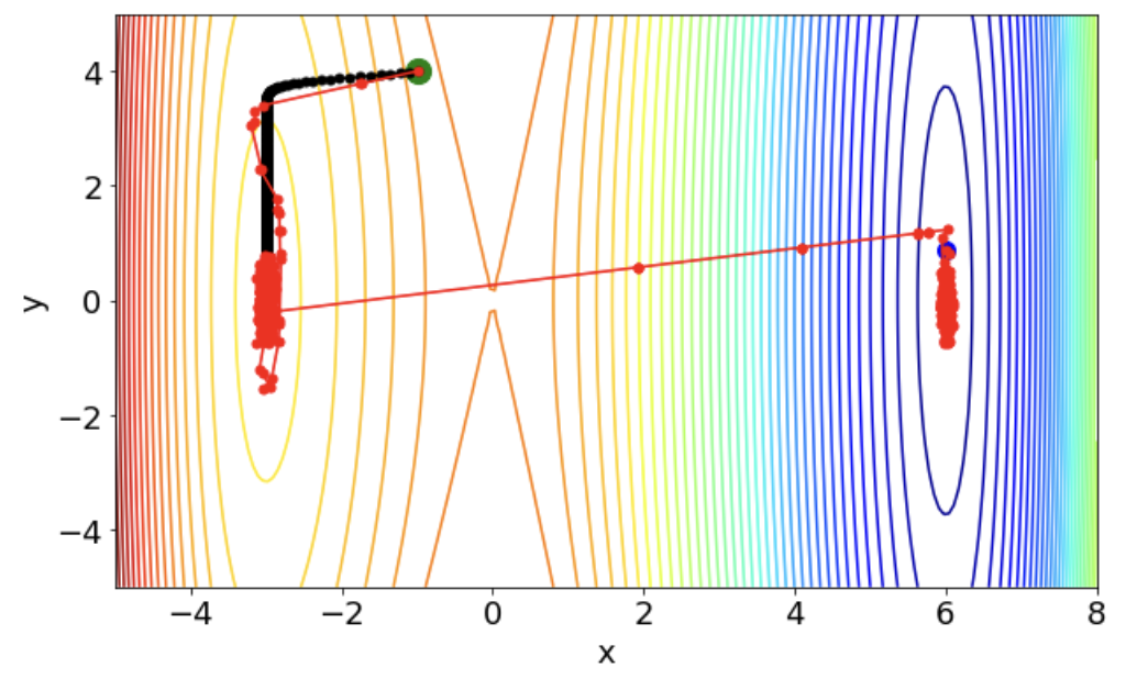
Figure 1. The comparison of the trajectories of SGD (with a fixed learning rate) and Poisson SGD (with the random learning rate) in optimizing the function $z=x^{4}-4x^{3}-36x^{2}+y^{2}$. The point $(-3,0)$ represents a local minimum and the point $(6,0)$ is identified as the global minimum. A green point indicates the initial position, a black line represents the trajectory of SGD, and a red line represents the trajectory of Poisson SGD.

4. Convergence Theory for Poisson SGD

We provide theoretical results on the convergence of Poisson SGD (Algorithm 1). Our main interest is a distribution of the generated parameter $\theta_{K}$ by Poisson SGD associated with the empirical risk minimization problem (2).

4.1. Stationary Distribution of Poisson SGD

In this section, we show that the parameter $\theta_{K}$ by the Poisson SGD follows a stationary distribution. Formally, we define the stationary distribution of the Markov process. In preparation, we utilize the notion of transition probability $Q(\theta,dw)$ from a distribution $p_{0}(\theta)$ to another $p_{1}(\theta)$ on $\Theta$, that is, $p_{1}(w)=\int_{\Theta}Q(\theta,dw)p_{0}(d\theta)$ holds.

Definition 1.

Let $Q(\theta,dw)$ be the transition probability of a Markov process in $\Theta$. If the following equation holds, we call the probability distribution $\pi(\theta)$ stationary distribution of the Markov process:

$$\pi(dw)=\int_{\Theta}Q(\theta,dw)\pi(d\theta).$$

A stationary distribution is an useful notion to represent a limit of the parameter distribution, and it enables us to analyze where the parameter converges by algorithms. For example, see the theoretical framework to analyze stochastic optimization algorithms by [32].

4.1.1. Assumption

We provide several principal assumptions. First, we consider the basis assumptions on the loss function $\ell(\cdot;\cdot)$. The following conditions are fairly general for the analysis of stochastic optimization algorithms, e.g. [1].

Assumption 1 (Loss function).

The loss function $\ell:\mathcal{Z}\times\Theta\to\mathbb{R}_{\geq 0}$ satisfies the following conditions:

• $\ell(z;\theta)$ is absolutely continuous and differentiable with respect to $\theta\in\Theta$ for every $z\in\mathcal{Z}$.

• $\nabla_{\theta}\ell(z;\theta)$ is continuous in $\theta$ and $z$ for all $\theta\in\Theta$ and $z\in\mathcal{Z}$.

The first condition is satisfied by a large class of models, such as linear regression model, or deep neural networks whose activation function is ReLU or sigmoid function. From the second condition, we define an upper bound $M_{\ell}:=\max_{\theta\in\Theta,z\in\mathcal{Z}}\|\nabla_{\theta}\ell(z;\theta)\|$ since $\Theta$ and $\mathcal{Z}$ are compact.

4.1.2. Statement of Convergence

Let $\mu_{\textbf{z},K}$ be a distribution of the output $\theta_{K}$ from the Poisson SGD in Algorithm 1 with the given dataset z. We discuss the convergence of $\mu_{\textbf{z},K}$ as $K$ increases.

In preparation, we define a probability measure on $\Theta$ for arbitrary $\beta,\varepsilon>0$, whose density is written as follows:

$$\mu_{\textbf{z}}^{(\beta,\varepsilon)}(d\theta)\propto\left(\beta M_{\ell}+\frac{1}{\varepsilon}+a_{d}\beta\|\nabla L_{\textbf{z}}(\theta)\|\right)\exp(-\beta L_{\textbf{z}}(\theta))d\theta,$$ (9)

where $a_{d}:={\Gamma(d/2)}/({\sqrt{\pi}\Gamma(d/2+1/2)})$. The probability measure (9) is concentrated around the global minima of $L_{\textbf{z}}(\theta)$, since the dominant exponential term $\exp(-\beta L_{\textbf{z}}(\theta))$ in (9) increases in $L_{\textbf{z}}(\theta)$. In addition, as the inverse temperature parameter $\beta$ increases, the measure $\mu_{\textbf{z}}^{(\beta,\varepsilon)}$ concentrates more around the global minimum.

We show our results on the convergence of the stationary distribution. The discrepancy is measured by the Wasserstein distance $\mathcal{W}_{1}(\cdot,\cdot)$. We remark that this theorem is the integration of Theorem 3 and Theorem 4 appearing later in Section 5. Recall that we defined $W:=\mathrm{diam}(\Theta)$.

Theorem 1 (Stationary distribution of Poisson SGD).

Fix arbitrary $\beta,\varepsilon>0$. Suppose Assumption 1 holds. We set the hyper-parameter of Poisson SGD as $C_{P}={1}/{\varepsilon}$. Then, for any $K\in\mathbb{N}$, the distribution $\mu_{\textbf{z},K}$ satisfies

$$\mathcal{W}_{1}(\mu_{\textbf{z},K},\mu_{\textbf{z}}^{(\beta,\varepsilon)})\leq 4\sqrt{d}K\varepsilon+W\cdot\kappa(\beta,\varepsilon,d)^{K},$$ (10)

where $0<\kappa(\beta,\varepsilon,d)<1$ is a constant.

Moreover, if $\kappa(\beta,\varepsilon,d)$ satisfies $\lim_{K\rightarrow\infty}\kappa(\beta,\delta/K,d)^{K}=0$ with some $\delta>0$, there exists a sequence $\varepsilon=\varepsilon_{K}\searrow 0$ as $K\to\infty$ such that $\mathcal{W}_{1}(\mu_{\textbf{z},K},\mu_{\textbf{z}}^{(\beta,\varepsilon)})=o(1)$ as $K\to\infty$ holds.

This theorem shows that the parameter distribution $\mu_{\textbf{z},K}$ by Poisson SGD converges to the stationary distribution $\mu_{\textbf{z}}^{(\beta,\varepsilon)}$ owing to the random learning rate (7). This is contrast to ordinary SGD, which is not shown to converge to a stationary distribution. Further, Poisson SGD does not make any assumptions on the gradient noise $\xi_{k}^{(n,m)}$ in Remark 1, unlike SGLD, which converges to a stationary distribution by introducing Gaussianity in the gradient noise.

The right-hand side in (10) shows an approximation-complexity trade-off of Poisson SGD described as follows. In preparation, we will introduce a certain stochastic process to achieve the stationary distribution $\mu_{\textbf{z}}^{(\beta,\varepsilon)}$ (detail is in Section 5). The first term of (10) describes an approximation error of Poisson SGD to the stochastic process. The second term of (10) denotes a convergence error of the stochastic process to the stationary distribution $\mu_{\textbf{z}}^{(\beta,\varepsilon)}$, which reflects the complexity of the stochastic process. $\varepsilon$ is a parameter for the stochastic process and controls the balance between the approximation error and the complexity error.

We further discuss the additional assumption $\lim_{K\rightarrow\infty}\kappa(\beta,\delta/K,d)^{K}=0$. This condition is related to the convergence rate of the approximated stochastic process of Poisson SGD. Although the explicit form of $\kappa(\beta,\delta/K,d)$ is not clarified in our case, there is a common example having its explicit form. One example is SGLD: [32] shows that a form of $\kappa(\beta,\delta/K,d)$ can be calculated, because SGLD is reduced to the Langevin process.

Remark 2 (Comparison with SGLD).

We discuss the difference between Poisson SGD and SGLD, which is another method achieving a stationary distribution. First, while SGLD adds a Gaussian noise to the update formula of SGD, Poisson SGD does not have an additive noise. The second difference is the form of the stationary distribution. A stationary distribution of SGLD is the Gibbs distribution, and that of Poisson SGD has the different form (9). This difference is derived from the random learning rate of Poisson SGD.

4.2. Global Convergence

We discuss the global convergence statement, that is, the empirical risk $L_{\textbf{z}}(\theta_{K})$ with Poisson SGD is minimized with high probability. We consider the additional assumption for the loss function $\ell$:

Assumption 2.

With some $c_{1}>0$, $\sup_{z\in\mathcal{Z}}\|\nabla\ell(z;\theta_{1})-\nabla\ell(z;\theta_{2})\|\leq c_{1}\|\theta_{1}-\theta_{2}\|$ holds for every $\theta_{1}\neq\theta_{2}\in\Theta$.

Then, we obtain the following global convergence theorem. We define $B:=\sup_{z\in\mathcal{Z}}\|\nabla\ell(z;0)\|$ by following Assumption 1.

Theorem 2 (Global convergence of Poisson SGD on empirical risk).

Fix arbitrary $\beta,\varepsilon>0$. Consider Poisson SGD in which $C_{P}={1}/{\varepsilon}$. Let the upper bound of $\mathcal{W}_{1}(\mu_{\textbf{z},K},\mu_{\textbf{z}}^{(\beta,\varepsilon)})$ obtained in Theorem 1 be $d_{K}(\beta,\varepsilon,d)$. Also, suppose that Assumption 1 and 2 hold. Then, it holds that

$$\mathbb{E}_{\theta_{K}\sim\mu_{\textbf{z},K}}[L_{\textbf{z}}(\theta_{K})]-\min_{\theta\in\Theta}L_{\textbf{z}}(\theta)$$ (11)

$$\leq (c_{1}W+B)\sqrt{Wd_{K}(\beta,\varepsilon,d)}+\frac{1}{\beta}\left(\frac{d}{2}\log\frac{eW^{2}c_{1}\beta}{d}+\log\left(1+\frac{a_{d}(c_{1}W+B)}{M_{\ell}}\right)\right).$$ (12)

Theorem 2 states that we can make $\mathbb{E}[L_{\textbf{z}}(\theta_{K})]$ be arbitrarily close to $\min_{\theta\in\Theta}L_{\textbf{z}}(\theta)$ by selecting large $\beta$, provided that we can make $d_{K}(\beta,\varepsilon,d)$ arbitrarily small by the choice of $\varepsilon$ and $K$ in spite of $\beta$. Intuitively, Poisson SGD achieves global convergence by appropriately adjusting the learning rate and momentum coefficient based on the shape of the loss function at the current location. Poisson SGD achieves the global convergence by the similar approach of global convergence of SGLD by [32].

The right-hand side of (12) is divided into two terms. The first term expresses the distance between the parameter and its stationary distribution. The second represents the degree of concentration of the stationary distribution $\mu_{\textbf{z}}^{(\beta,\varepsilon)}$ on the global optima. The higher the inverse temperature $\beta$, the more the term decreases.

5. Proof Outline

5.1. Overview

We give an overview of a proof of Theorem 1. In preparation, we present several key concepts: (i) the property of the piece-wise deterministic Markov process (PDMP) [11, 12], and (ii) the ergodicity of bouncy particle sampler (BPS) [29]. The PDMP is a class of Markov processes that behave deterministically for some period and jumps randomly, which easily converges to a stationary distribution. BPS is a stochastic algorithm in the class of the PDMP.

We show the statement by the following steps:

1. We show that the distribution of the parameter by Poisson SGD is sufficiently close to that of a parameter by BPS. We show this claim by using the approximation theory on PDMP (Theorem 3).

2. We derive a stationary distribution and the ergodicity of BPS, following previous researches (Theorem 4).

5.2. Design of BPS

We introduce BPS, which is one of the most popular algorithms in PDMPs, and actively studied in terms of MCMC algorithm [13, 2]. BPS generates a sequence of parameters $\{\widehat{\theta}_{k}\}_{k=1}^{K}\subset\Theta$ and velocity vectors $\{\widehat{v}_{k}\}_{k=1}^{K}\subset\mathbb{R}^{d}$ in its recursive manner, as shown in Algorithm 2. Let $(\widehat{\theta}_{0},\widehat{v}_{0})$ be the initialization. For the $k$-th iteration, BPS generates a learning rate $\widehat{\eta}_{k}$ from an exponential distribution whose intensity depends on the previous pair $(\widehat{\theta}_{k-1},\widehat{v}_{k-1})$ and the positive constants $\Lambda_{\mathrm{ref}}$ and $C_{B}$. After obtaining the parameter $\widehat{\theta}_{k}$, we consider the stochastic update of the velocity vector. That is, with the probability

$$\widehat{p}_{k}:=\frac{\beta\langle\nabla L_{\textbf{z}}(\widehat{\theta}_{k}),\widehat{v}_{k-1}\rangle_{+}+C_{B}}{\beta\langle\nabla L_{\textbf{z}}(\widehat{\theta}_{k}),\widehat{v}_{k-1}\rangle_{+}+\Lambda_{\mathrm{ref}}+C_{B}},$$ (13)

we update the velocity vector with the gradient of the full-batch loss $\nabla L_{\textbf{z}}$, otherwise with the sample from the uniform distribution on $\mathbb{S}^{d-1}$. The former update is called reflection, and the latter is refreshment. We remark that $\|\widehat{v}_{k}\|$ is constant for $k=1,2,...,K$ in the same way as Poisson SGD (See Proposition 7 in Appendix).

Algorithm 2 Bouncy Particle Sampler

1:  Initialize $(\widehat{\theta}_{0},\widehat{v}_{0})$ as $\|\widehat{v}_{0}\|=1$.

2:  for $k=1,2,...,K$ do

3:     Sample $\widehat{\eta}_{k}$ as $\widehat{\eta}_{k}\sim P(\widehat{\eta}_{k}\geq t)=\exp\left(-\int_{0}^{t}\{\beta\langle\nabla L_{\textbf{z}}(\widehat{\theta}_{k-1}+r\widehat{v}_{k-1}),\widehat{v}_{k-1}\rangle_{+}+\Lambda_{\mathrm{ref}}+C_{B}\}dr\right)$

4:     Update $\widehat{\theta}_{k}$ as $\widehat{\theta}_{k}=\widehat{\theta}_{k-1}+\widehat{\eta}_{k}\widehat{v}_{k-1}$

5:     With probability $\widehat{p}_{k}$ as (13), update $\widehat{v}_{k}$ as

$$\widehat{v}_{k}=\widehat{v}_{k-1}-2\frac{\langle\nabla L_{\textbf{z}}(\widehat{\theta}_{k}),\widehat{v}_{k-1}\rangle}{\|\nabla L_{\textbf{z}}(\widehat{\theta}_{k})\|^{2}}\nabla L_{\textbf{z}}(\widehat{\theta}_{k})$$

Otherwise, update $\widehat{v}_{k}$ as

$$\widehat{v}_{k}\sim\mathrm{Unif}(\mathbb{S}^{d-1})$$

6:  end for

7:  Return $(\widehat{\theta}_{K},\widehat{v}_{K})$

5.3. Connect Poisson SGD and BPS

We show that the output distribution of Poisson SGD and that of BPS are sufficiently close as in the following statement:

Theorem 3 (Distance between Poisson SGD and BPS).

Fix arbitrary $\beta,\varepsilon>0$. As for Poisson SGD, we set $C_{P}={1}/{\varepsilon}$. As for BPS, we set $\Lambda_{\mathrm{ref}}$ and $C_{B}$ as $\Lambda_{\mathrm{ref}}+C_{B}=\beta M_{\ell}+{1}/{\varepsilon}$. Let the distribution of the obtained parameter by Poisson SGD and BPS be $\mu_{\textbf{z},K}$ and $\widehat{\mu}_{\textbf{z},K}$ respectively. We set the same initial value between Poisson SGD and BPS. Then, the following holds:

$$\mathcal{W}_{1}(\mu_{\textbf{z},K},\widehat{\mu}_{\textbf{z},K})\leq 4\sqrt{d}K\varepsilon.$$ (14)

For proving this theorem, we calculate the distance between Poisson SGD and BPS by a one-step update. Then, we simply accumulate this error for $K$ times. In this discussion, we mainly use the property that if learning rate $\eta_{k}$ and $\widehat{\eta}_{k}$ are small, the difference of $v_{k}$ and $\widehat{v}_{k}$ is also made to be small. This type of discussion is also used in [32].

5.4. The Stationary Distribution and Ergodicity of BPS

In this section, we investigate the stationary distribution and ergodicity of BPS. First, we define the term ergodicity.

Definition 2 (Ergodicity).

We consider the discrete-time Markov process. If the process converges to a unique stationary distribution, we call the process has the ergodicity. Especially, if the ergodic process converges to its stationary distribution by the exponential rate about the number of iteration $k$, the process is called exponentially ergodic.

Without ergodicity, the stochastic process may converge to more than one stationary distribution, or not converge to any stationary distribution due to stacking to a saddle point in the parameter space. So we have to prove this property when we try to analyze the stationary distribution of a stochastic process.

Now, we show our result about BPS.

Theorem 4 (Stationary Distribution of BPS).

Suppose that Assumption 1 holds. Set the parameter of BPS, $\Lambda_{\mathrm{ref}}$ and $C_{B}$ as in Theorem 3. Then, the distribution $\widehat{\mu}_{\textbf{z},K}$ of the obtained parameters $\widehat{\theta}_{K}$ by BPS satisfies the following:

$$\|\widehat{\mu}_{\textbf{z},K}-\mu_{\textbf{z}}^{(\beta,\varepsilon)}\|_{\mathrm{TV}}\leq\kappa(\beta,\varepsilon,d)^{K},$$ (15)

where $\kappa(\beta,\varepsilon,d)$ is a positive constant less than $1$.

In the proof of this theorem, we use the discussion in [13] which showed that continuous-time BPS converges to the unique stationary distribution $\pi(\theta)\propto\exp(-U(\theta))$ by the exponential rate in TV distance.

6. Generalization Error Analysis

We define an expected risk of $\theta\in\Theta$, also known as the generalization error

$$L(\theta):=\mathbb{E}_{z\sim P_{*}}[\ell(z;\theta)],$$

which measures a prediction performance with unseen data. We calculate the generalization error of the parameter obtained by the Poisson SGD, using the discussion in [32].

Now, we give our results. We define $A:=\sup_{z\in\mathcal{Z}}|\ell(z;0)|$ by following Assumption 1.

Theorem 5 (Generalization Error of Poisson SGD).

Suppose that Assumption 1 and 2 hold. Let $\theta_{K}$ be the parameter obtained by Poisson SGD with $C_{P}={1}/{\varepsilon}$. Then, we obtain the following bound:

$$\mathbb{E}_{\textbf{z}\sim P_{*}^{n}}[\mathbb{E}_{\theta_{K}\sim\mu_{\textbf{z},K}}[L(\theta_{K})]]-\min_{\theta\in\Theta}L(\theta)$$ (16)

$$\leq (c_{1}W+B)\left(\sqrt{Wd_{K}(\beta,\varepsilon,d)}+2W\left(\left(\frac{C_{d}+\beta C}{n}\right)^{\frac{1}{2}}+\left(\frac{C_{d}+\beta C}{n}\right)^{\frac{1}{4}}\right)\right)$$ (17)

$$+ \frac{1}{\beta}\left(\frac{d}{2}\log\frac{eW^{2}c_{1}\beta}{d}+\log\left(1+\frac{a_{d}(c_{1}W+B)}{M_{\ell}}\right)\right),$$ (18)

where $d_{K}(\beta,\varepsilon,d)$ is the upper bound of the Wasserstein distance in Theorem 1, $C_{d}={4a_{d}(c_{1}W+B)}/{M_{\ell}}$, and $C=c_{1}W^{2}+2BW+2A$.

Theorem 5 states that the expected value of the generalization error of Poisson SGD can be arbitrarily close to its global optima in $\theta\in\Theta$, by selecting small $\varepsilon$, large $K$, large $\beta$, and large $n$, provided that $d_{K}(\beta,\varepsilon,d)$ can be arbitrarily small only by the choice of $\varepsilon$ and $K$.

We further discuss a way of improve an order of the generalization bound in Theorem 5. While our bound has the order $O((1/n)^{1/4})$, we can obtain an order $O(1/n)$ by using the dissipativity condition of the loss function, which is used in [32] for SGLD. The dissipativity condition allows us to derive log-Sobolev inequality for $L_{\textbf{z}}(\theta)$, which leads the improved sample complexity. We state this fact in the following proposition.

Proposition 6.

Suppose that the same condition and setting as Theorem 5 hold. In addition, we assume that the Gibbs distribution $\nu_{\textbf{z}}^{(\beta)}\propto\exp(-\beta L_{\textbf{z}}(\theta))$ satisfies the log-Sobolev inequality for any dataset $\textbf{z}=\{z_{1},...,z_{n}\}$, that is,

$$\mathbb{E}[f(\theta)^{2}\log f(\theta)^{2}]-\mathbb{E}[f(\theta)^{2}]\log\mathbb{E}[f(\theta)^{2}]\leq c_{\mathrm{LS}}^{(\beta)}\mathbb{E}[\|\nabla f(\theta)\|^{2}]\,$$ (19)

holds for all smooth functions $f$ and any data $\textbf{z}=\{z_{1},...,z_{n}\}$, where $\theta\sim\nu_{\textbf{z}}^{(\beta)}$ and $c_{\mathrm{LS}}^{(\beta)}<\infty$ is a constant. Then, the following holds:

$$\mathbb{E}_{\textbf{z}\sim P_{*}^{n}}[\mathbb{E}_{\theta_{K}\sim\mu_{\textbf{z},K}}[L(\theta_{K})]]-\min_{\theta\in\Theta}L(\theta)$$ (20)

$$\leq (c_{1}W+B)\left(\sqrt{Wd_{K}(\beta,\varepsilon,d)}+\frac{2c_{\mathrm{LS}}^{(\beta)}\beta M_{\ell}}{n}\right)+W\sqrt{2c_{\mathrm{LS}}^{(\beta)}\log\left(1+a_{d}\beta\varepsilon M_{\ell}\right)}+\frac{d}{2\beta}\log\left(\frac{eW^{2}c_{1}\beta}{d}\right).$$ (21)

7. Conclusion

We developed a new variant of SGD, Poisson SGD, whose search direction degenerates and derived its stationary distribution by incorporating a modification on the learning rate. The parameters trained by Poisson SGD are close enough to the global minima to take advantage of convergence to the stationary distribution. The generalization error is also evaluated. We believe that our work leads to the analysis of the actual SGD dynamics, not variants of it in the future.

Appendix A Supportive Information

We verify that the velocity vector is normalized by the choice of the momentum coefficient for Poisson SGD and BPS.

Proposition 7.

Consider the update (5) for $v_{k}$ with its momentum coefficient (8). Then, for $\forall k\in\{1,2,...,K\}$, we have $\|v_{k}\|=1$. Further, for $\widehat{v}_{k}$ defined in Algorithm 2, we obtain $\|\widehat{v}_{k}\|=1$ for every $k=1,...,K$.

Proof.

We first consider $v_{k}$ with the Poisson SGD case. Simply, we have

$$\|v_{k}\|= \left\|v_{k-1}-2\frac{\langle\nabla\widehat{L}_{\textbf{z}}^{(k)}(\theta_{k}),v_{k-1}\rangle}{\|\nabla\widehat{L}_{\textbf{z}}^{(k)}(\theta_{k})\|^{2}}\nabla\widehat{L}_{\textbf{z}}^{(k)}(\theta_{k})\right\|$$ (22)

$$= \left\|\left(I_{d}-2\frac{\nabla\widehat{L}_{\textbf{z}}^{(k)}(\theta_{k})\nabla\widehat{L}_{\textbf{z}}^{(k)}(\theta_{k})^{\top}}{\|\nabla\widehat{L}_{\textbf{z}}^{(k)}(\theta_{k})\|^{2}}\right)v_{k-1}\right\|$$ (23)

$$= \sqrt{v_{k-1}^{\top}\left(I_{d}-2\frac{\nabla\widehat{L}_{\textbf{z}}^{(k)}(\theta_{k})\nabla\widehat{L}_{\textbf{z}}^{(k)}(\theta_{k})^{\top}}{\|\nabla\widehat{L}_{\textbf{z}}^{(k)}(\theta_{k})\|^{2}}\right)^{2}v_{k-1}}$$ (24)

$$= \|v_{k-1}\|.$$ (25)

Since we set $\|v_{0}\|=1$ for initialization, the statement holds.

For $\widehat{v}_{k}$ with the BPS case, the reflection does not change the norm of $\widehat{v}_{k}$ in the same way, and the refreshment also keeps $\|\widehat{v}_{k}\|=1$, which completes the proof. ∎

Appendix B Proof of Theorem 1

Proof.

By Theorem 3 and 4, we can bound the approximation error

$$\mathcal{W}_{1}(\mu_{\textbf{z},K},\widehat{\mu}_{\textbf{z},K})\leq 4\sqrt{d}K\varepsilon,$$ (26)

and the convergence error of BPS as

$$\|\widehat{\mu}_{\textbf{z},K}-\mu_{\textbf{z}}^{(\beta,\varepsilon)}\|_{\mathrm{TV}}\leq\kappa(\beta,\varepsilon,d)^{K}.$$ (27)

From Theorem 4 in [18], we can bound the Wasserstein distance by the total variation, then obtain

$$\mathcal{W}_{1}(\widehat{\mu}_{\textbf{z},K},\mu_{\textbf{z}}^{(\beta,\varepsilon)})\leq W\|\widehat{\mu}_{\textbf{z},K}-\mu_{\textbf{z}}^{(\beta,\varepsilon)}\|_{\mathrm{TV}}\leq W\kappa(\beta,\varepsilon,d)^{K}.$$ (28)

The triangle inequality completes the proof. ∎

Appendix C Proof of Theorem 3

Proof.

From the definition of Wasserstein distance,

$$\mathcal{W}_{1}(\mu_{\textbf{z},k},\widehat{\mu}_{\textbf{z},k})=\inf_{\pi\in\Pi(\mu_{\textbf{z},k},\widehat{\mu}_{\textbf{z},k})}\mathbb{E}_{\pi}[\|\theta_{k}-\widehat{\theta}_{k}\|_{1}]$$

holds, so we study the distance between $\theta_{k}$ and $\widehat{\theta}_{k}$ in terms of the norm $\|\cdot\|_{1}$. Since $\|v_{k}\|=\|v_{k-1}\|=\|\widehat{v}_{k}\|=\|\widehat{v}_{k-1}\|=1$ holds by Proposition 7, we have

$$\mathbb{E}_{\pi}[\|\theta_{k}-\widehat{\theta}_{k}\|_{1}]= \mathbb{E}_{\pi}[\|\theta_{k-1}+\eta_{k}v_{k-1}-(\widehat{\theta}_{k-1}+\widehat{\eta}_{k}\widehat{v}_{k-1})\|_{1}]$$

$$\leq \mathbb{E}_{\pi}[\|\theta_{k-1}-\widehat{\theta}_{k-1}\|_{1}]+\mathbb{E}_{\pi}[\|(\widehat{\eta}_{k}-\eta_{k})\widehat{v}_{k-1}+\eta_{k}(\widehat{v}_{k-1}-v_{k-1})\|_{1}]$$

$$\leq \mathbb{E}_{\pi}[\|\theta_{k-1}-\widehat{\theta}_{k-1}\|_{1}]+\mathbb{E}_{\pi}[\|(\widehat{\eta}_{k}-\eta_{k})\widehat{v}_{k-1}\|_{1}]+\mathbb{E}_{\pi}[\|\eta_{k}(\widehat{v}_{k-1}-v_{k-1})\|_{1}]$$

$$\leq \mathbb{E}_{\pi}[\|\theta_{k-1}-\widehat{\theta}_{k-1}\|_{1}]+\sqrt{d}\mathbb{E}_{\pi}[|\eta_{k}-\widehat{\eta}_{k}|]+2\sqrt{d}\mathbb{E}_{\pi}[\eta_{k}],$$ (29)

where we use $\|\cdot\|_{1}\leq\sqrt{d}\|\cdot\|$ in the last inequality.

We first evaluate the second term of (C). There exists a coupling $\pi$ such that

$$\mathbb{E}_{\pi}[|\eta_{k}-\widehat{\eta}_{k}|]=\mathcal{W}_{1}(P_{\eta_{k}},P_{\widehat{\eta}_{k}})$$

holds, where $P_{\eta_{k}}$ and $P_{\widehat{\eta}_{k}}$ denote the distribution of $\eta_{k}$ and $\widehat{\eta}_{k}$ respectively. We use such a coupling as $\pi$. In evaluating $\mathcal{W}_{1}(P_{\eta_{k}},P_{\widehat{\eta}_{k}})$, we consider the following analysis. $\eta_{k}$ and $\widehat{\eta}_{k}$ are 1-dimensional and their cumulative distribution function is written as

$$F_{1}(t)=1-\exp\left(-\int_{0}^{t}(\beta\langle\nabla\widehat{L}_{\textbf{z}}^{(k)}(\theta+rv),v\rangle_{+}+C_{P})dr\right),$$ (30)

$$F_{2}(t)=1-\exp\left(-\int_{0}^{t}(\beta\langle\nabla L_{\textbf{z}}(\theta+rv),v\rangle_{+}+C_{B}+\Lambda_{\mathrm{ref}})dr\right),$$ (31)

respectively, and we also have

$$\beta\langle\nabla\widehat{L}_{\textbf{z}}^{(k)}(\theta+rv),v\rangle_{+}+C_{P}\geq C_{P},$$ (32)

$$\beta\langle\nabla L_{\textbf{z}}(\theta+rv),v\rangle_{+}+C_{B}+\Lambda_{\mathrm{ref}}\geq C_{B}+\Lambda_{\mathrm{ref}},\mbox{~{}and~{}}$$ (33)

$$|(\beta\langle\nabla\widehat{L}_{\textbf{z}}^{(k)}(\theta+rv),v\rangle_{+}+C_{P})-(\beta\langle\nabla L_{\textbf{z}}(\theta+rv),v\rangle_{+}+C_{B}+\Lambda_{\mathrm{ref}})|$$ (34)

$$\leq\max\{|-\beta M_{\ell}+C_{P}-(C_{B}+\Lambda_{\mathrm{ref}})|,|\beta M_{\ell}+C_{P}-(C_{B}+\Lambda_{\mathrm{ref}})|\}.$$ (35)

Hence, we can use Lemma 8 and obtain

$$\mathcal{W}_{1}(P_{\eta_{k}},P_{\widehat{\eta}_{k}})\leq\frac{\max\{|-\beta M_{\ell}+C_{P}-(C_{B}+\Lambda_{\mathrm{ref}})|,|\beta M_{\ell}+C_{P}-(C_{B}+\Lambda_{\mathrm{ref}})|\}}{C_{P}(C_{B}+\Lambda_{\mathrm{ref}})}.$$ (36)

Next, we evaluate the third term of (C). We have

$$\mathbb{E}[\eta_{k}]= \int_{0}^{\infty}P(\eta_{k}\geq t)dt$$

$$= \int_{0}^{\infty}\exp\left(-\int_{0}^{t}\{\beta\langle\nabla\widehat{L}^{(k)}_{\textbf{z}}(\theta_{k-1}+rv_{k-1}),v_{k-1}\rangle_{+}+C_{P}\}dr\right)dt$$

$$\leq \int_{0}^{\infty}\exp\left(-C_{P}t\right)dt$$

$$= \frac{1}{C_{P}}.$$ (37)

Substituting (36) and (C) into (C), we have

$$\mathbb{E}_{\pi}[\|\theta_{k}-\widehat{\theta}_{k}\|_{1}]\leq \mathbb{E}_{\pi}[\|\theta_{k-1}-\widehat{\theta}_{k-1}\|_{1}]$$ (38)

$$+ \frac{\sqrt{d}\max\{|-\beta M_{\ell}+C_{P}-(C_{B}+\Lambda_{\mathrm{ref}})|,|\beta M_{\ell}+C_{P}-(C_{B}+\Lambda_{\mathrm{ref}})|\}}{C_{P}(C_{B}+\Lambda_{\mathrm{ref}})}+\frac{2\sqrt{d}}{C_{P}}.$$ (39)

Since we take $C_{P}$ in Poisson SGD as $C_{P}={1}/{\varepsilon}$ and $C_{B}$ and $\Lambda_{\mathrm{ref}}$ in BPS as $C_{B}+\Lambda_{\mathrm{ref}}=\beta M_{\ell}+{1}/{\varepsilon}$, (38) can be written as

$$\mathbb{E}_{\pi}[\|\theta_{k}-\widehat{\theta}_{k}\|_{1}]\leq \mathbb{E}_{\pi}[\|\theta_{k-1}-\widehat{\theta}_{k-1}\|_{1}]+4\sqrt{d}\varepsilon.$$ (40)

Hence, solving this recursive inequality with $\theta_{0}=\widehat{\theta}_{0}$, we have

$$\mathbb{E}_{\pi}[\|\theta_{K}-\widehat{\theta}_{K}\|_{1}]\leq 4\sqrt{d}K\varepsilon,$$ (41)

which is the desired conclusion. ∎

Lemma 8.

Let $a_{1}$ and $a_{2}$ be $\mathbb{R}$-valued random variables whose cumulative distribution functions are

$$F_{1}(t)=1-\exp\left(-\int_{0}^{t}f_{1}(r)dr\right),\mbox{~{}and~{}}F_{2}(t)=1-\exp\left(-\int_{0}^{t}f_{2}(r)dr\right),$$ (42)

respectively, where $f_{1},f_{2}:\mathbb{R}\rightarrow\mathbb{R}$ are continuous functions. Let the distributions of $a_{1}$ and $a_{2}$ be $P_{1}$ and $P_{2}$ respectively. Suppose that there exists $M,m_{1},m_{2}>0$ such that $|f_{2}(t)-f_{1}(t)|\leq M$, $m_{1}\leq f_{1}(t)$, and $m_{2}\leq f_{2}(t)$ hold for $\forall t\in\mathbb{R}$. Then, the Wasserstein distance between $P_{1}$ and $P_{2}$ satisfies

$$\mathcal{W}_{1}(P_{1},P_{2})\leq\frac{M}{m_{1}m_{2}}.$$ (43)

Proof.

Since $a_{1}$ and $a_{2}$ are 1-dimensional, we have

$$\mathcal{W}_{1}(P_{1},P_{2})=\int_{0}^{1}\left|F_{1}^{-1}(q)-F_{2}^{-1}(q)\right|dq.$$ (44)

We introduce several notation $\delta(r)=f_{2}(r)-f_{1}(r)$, $t=F_{1}^{-1}(q)$, and $t^{\prime}=F_{2}^{-1}(q)$, then

$$\int_{0}^{t}f_{1}(r)dr=\log\frac{1}{1-q}$$ (45)

$$\int_{0}^{t^{\prime}}(f_{1}(r)+\delta(r))dr=\log\frac{1}{1-q}$$ (46)

holds. So, we obtain

$$\int_{t^{\prime}}^{t}f_{1}(r)dr=\int_{0}^{t^{\prime}}\delta(r)dr.$$ (47)

Hence, we have

$$\left|\int_{t^{\prime}}^{t}f_{1}(r)dr\right|=\int_{\min\{t,t^{\prime}\}}^{\max\{t,t^{\prime}\}}f_{1}(r)dr\leq Mt^{\prime}.$$ (48)

In addition, $\int_{\min\{t,t^{\prime}\}}^{\max\{t,t^{\prime}\}}f_{1}(r)dr\geq m_{1}|t-t^{\prime}|$ holds, so we have

$$|t-t^{\prime}|\leq\frac{Mt^{\prime}}{m_{1}}.$$ (49)

We have the upper bound of $t^{\prime}$ as

$$\log\frac{1}{1-q}=\int_{0}^{t^{\prime}}f_{2}(r)dr\geq m_{2}t^{\prime},$$ (50)

so we have

$$|t-t^{\prime}|\leq\frac{M}{m_{1}m_{2}}\log\frac{1}{1-q}.$$ (51)

Since $\int_{0}^{1}|\log(1-q)|dq=1$ holds, we obtain

$$\int_{0}^{1}\left|F_{1}^{-1}(q)-F_{2}^{-1}(q)\right|dq\leq\frac{M}{m_{1}m_{2}}.$$ (52)

∎

Appendix D Proof of Theorem 4

We prove this theorem by two steps. First, we prove that BPS has $\mu_{\textbf{z}}^{(\beta,\varepsilon)}$ as one of its stationary distributions in section D.1. At this stage, BPS may have other forms of stationary distribution or may not converge to its stationary distribution. Second, we prove that BPS has a unique stationary distribution and converges to its stationary distribution at exponential rate, in other words, it has the exponential ergodicity, in section D.2.

D.1. The form of the stationary distribution

In this section, we check that BPS has $\mu_{\textbf{z}}^{(\beta,\varepsilon)}$ as a stationary distribution. In the proof, we define $\lambda(\theta,v):=\beta\langle\nabla L_{\textbf{z}}(\theta),v\rangle_{+}$, $\bar{\lambda}(\theta,v):=\lambda(\theta,v)+\Lambda_{\mathrm{ref}}$, and $R_{\textbf{z}}(\theta):=I_{d}-2\frac{\nabla L_{\textbf{z}}(\theta)\nabla L_{\textbf{z}}(\theta)^{\top}}{\|\nabla L_{\textbf{z}}(\theta)\|^{2}}$. We remark that $R_{\textbf{z}}$ is a symmetric matrix and satisfies $R_{\textbf{z}}(\theta)^{2}=I_{d}$, so it is also an orthogonal matrix.

From the proof of Lemma 1 in the supplementary material of [13], we can write the transition probability $\widehat{Q}$ of BPS as following for arbitrary measurable sets $A\subset\Theta$ and $B\subset\mathbb{S}^{d-1}$:

$$\widehat{Q}((\theta,v),A\times B)= \int_{0}^{\infty}\exp\left\{-\int_{0}^{s}\left(\bar{\lambda}(\theta+uv,v)+C_{B}\right)du\right\}$$ (53)

$$\times\left(\bar{\lambda}(\theta+uv,v)+C_{B}\right)K((\theta+sv,v),A\times B)ds,$$ (54)

where a transition kernel $K$ is expressed as

$$K((\theta,v),A\times B)= \frac{\lambda(\theta,v)+C_{B}}{\bar{\lambda}(\theta,v)+C_{B}}\mathbbm{1}[\theta\in A]\mathbbm{1}[R_{\textbf{z}}(\theta)v\in B]$$ (55)

$$+ \frac{\Lambda_{\mathrm{ref}}}{\bar{\lambda}(\theta,v)+C_{B}}\mathbbm{1}[\theta\in A]\mu_{\mathrm{unif}}(B),$$ (56)

where $\mu_{\mathrm{unif}}$ is the uniform probability measure on $\mathbb{S}^{d-1}$.

Lemma 9.

Under Assumption 1, a probability measure on $\Theta\times\mathbb{S}^{d-1}$

$$\widehat{\mu}_{\textbf{z}}(A\times B)\propto\int_{A\times B}\left(\bar{\lambda}(\theta,-v)+C_{B}\right)\exp(-\beta L_{\textbf{z}}(\theta))d\theta\mu_{\mathrm{unif}}(dv)$$

is the stationary distribution induced from the transition probability $\widehat{Q}$ as (54).

Proof.

Our proof is almost the same as the proof of Lemma 1 in [13]. Let $\pi_{\textbf{z}}(d\theta,dv)=\exp(-\beta L_{\textbf{z}}(\theta))d\theta\mu_{\mathrm{unif}}(dv)$.

First, we prove

$$\int(\bar{\lambda}(\theta,v)+C_{B})\pi_{\textbf{z}}(d\theta,dv)K((\theta,v),A\times B)\propto\widehat{\mu}_{\textbf{z}}(A\times B).$$ (57)

Substituting (55), the left side of (57) is rewritten as

$$\int\pi_{\textbf{z}}(d\theta,dv)(\lambda(\theta,v)+C_{B})\mathbbm{1}[\theta\in A]\mathbbm{1}[R_{\textbf{z}}(\theta)v\in B]+\int\pi_{\textbf{z}}(d\theta,dv)\Lambda_{\mathrm{ref}}\mathbbm{1}[\theta\in A]\mu_{\mathrm{unif}}(B).$$ (58)

We consider changing the variable as $v^{\prime}=R_{\textbf{z}}(\theta)v$. Since $R_{\textbf{z}}(\theta)^{-1}=R_{\textbf{z}}(\theta)$ holds, we get $\lambda(\theta,R_{\textbf{z}}(\theta)^{-1}v^{\prime})=\lambda(\theta,-v^{\prime})$. In addition, since $|\mathrm{det}(R_{\textbf{z}}(\theta))|=1$, and $\mu_{\mathrm{unif}}(R_{\textbf{z}}(\theta)^{-1}dv^{\prime})=\mu_{\mathrm{unif}}(dv^{\prime})$ hold due to the rotational invariance of $\mu_{\mathrm{unif}}$, we obtain

$$\int_{A\times B}\pi_{\textbf{z}}(d\theta,dv^{\prime})(\lambda(\theta,-v^{\prime})+C_{B})+\int_{A\times B}\pi_{\textbf{z}}(d\theta,dv^{\prime})\Lambda_{\mathrm{ref}},$$

which is proportional to the right side of (57) from the definition of $\widehat{\mu}_{\textbf{z}}$.

Second, we prove $\int\widehat{Q}((\theta,v),(dy,dw))\widehat{\mu}_{\textbf{z}}(d\theta,dv)=\widehat{\mu}_{\textbf{z}}(dy,dw)$. We have

$$\int\widehat{Q}((\theta,v),(dy,dw))\widehat{\mu}_{\textbf{z}}(d\theta,dv)$$ (59)

$$\propto \int_{0}^{\infty}\exp\left(-\int_{0}^{s}\{\bar{\lambda}(\theta+uv,v)+C_{B}\}du\right)\{\bar{\lambda}(\theta+sv,v)+C_{B}\}$$ (60)

$$\times K((\theta+sv,v),(dy,dw))\{\bar{\lambda}(\theta,-v)+C_{B}\}\pi_{\textbf{z}}(d\theta,dv)ds.$$ (61)

If we change $\theta$ as $t=\theta+sv$, then this integral becomes

$$\int_{0}^{\infty}\exp\left(-\int_{0}^{s}\{\bar{\lambda}(t+(u-s)v,v)+C_{B}\}du\right)\{\bar{\lambda}(t,v)+C_{B}\}$$ (63)

$$\quad\times K((t,v),(dy,dw))\{\bar{\lambda}(t-sv,-v)+C_{B}\}\pi_{\textbf{z}}(d\theta,dv)ds.$$ (64)

Since $L_{\textbf{z}}(\theta)$ is absolutely continuous,

$$\exp(-\beta L_{\textbf{z}}(t-sv))=\exp\left(-\beta L_{\textbf{z}}(t)-\int_{0}^{s}\lambda(t-wv,-v)dw+\int_{0}^{s}\lambda(t-wv,v)dw\right)$$

holds in the same way as [13]. Substituting it into $\pi_{\textbf{z}}(dx,dv)$ and changing $u$ as $u-s=-w$,

$$\int_{0}^{\infty}\exp\left(-\int_{0}^{s}\{\bar{\lambda}(t-wv,-v)+C_{B}\}dw\right)\{\bar{\lambda}(t-sv,-v)+C_{B}\}ds$$ (66)

$$\times \{\bar{\lambda}(t,v)+C_{B}\}K((t,v),(dy,dw))\pi_{\textbf{z}}(dt,dv)$$ (67)

holds. The first line can be calculated as $\left[-\exp\left(-\int_{0}^{s}\{\bar{\lambda}(t-wv,-v)+C_{B}\}dw\right)\right]_{0}^{\infty}=1$, so it is equal to

$$\int\{\bar{\lambda}(t,v)+C_{B}\}K((t,v),(dy,dw))\pi_{\textbf{z}}(dt,dv).$$

Using (57), it is proportional to $\widehat{\mu}_{\textbf{z}}(dy,dw)$, which completes the proof. ∎

By the following proposition, we prove that $\mu_{\textbf{z}}^{(\beta,\varepsilon)}$ is one of the stationary distributions of BPS. Recall that we defined $a_{d}:={\Gamma(d/2)}/({\sqrt{\pi}\Gamma(d/2+1/2)})$.

Proposition 10.

The marginal distribution of the stationary distribution expressed in Lemma 9 is written as

$$\widehat{\mu}_{\textbf{z}}(d\theta)\propto(\Lambda_{\mathrm{ref}}+C_{B}+a_{d}\beta\|\nabla L_{\textbf{z}}(\theta)\|)\exp(-\beta L_{\textbf{z}}(\theta))d\theta.$$

Hence, if we put $\Lambda_{\mathrm{ref}}$ and $C_{B}$ as $\Lambda_{\mathrm{ref}}+C_{B}=\beta M_{\ell}+{1}/{\varepsilon}$, it corresponds to $\mu_{\textbf{z}}^{(\beta,\varepsilon)}$.

Proof.

We only need to integrate with $v$ the distribution $\widehat{\mu}_{\textbf{z}}$ expressed in Lemma 9. We have

$$\widehat{\mu}_{\textbf{z}}(d\theta)\propto \int_{v\in\mathbb{S}^{d-1}}(\Lambda_{\mathrm{ref}}+C_{B}+\beta\langle\nabla L_{\textbf{z}}(\theta),-v\rangle_{+})\exp(-\beta L_{\textbf{z}}(\theta))d\theta\mu_{\mathrm{unif}}(dv)$$ (68)

$$= (\Lambda_{\mathrm{ref}}+C_{B})\exp(-\beta L_{\textbf{z}}(\theta))d\theta+\exp(-\beta L_{\textbf{z}}(\theta))d\theta\beta\mathbb{E}_{v\sim\mu_{\mathrm{unif}}}[\langle\nabla L_{\textbf{z}}(\theta),v\rangle_{+}].$$ (69)

We can calculate the expected value in the last term as

$$\mathbb{E}_{v\sim\mu_{\mathrm{unif}}}[\langle\nabla L_{\textbf{z}}(\theta),v\rangle_{+}]=\mathbb{E}_{v\sim\mu_{\mathrm{unif}}}[\|\nabla L_{\textbf{z}}(\theta)\|(\cos{\phi})_{+}]=\|\nabla L_{\textbf{z}}(\theta)\|\mathbb{E}_{v\sim\mu_{\mathrm{unif}}}[(\cos{\phi})_{+}],$$ (70)

where $\phi\in\mathbb{R}$ is a random variable dependent on $v$ which satisfies

$$\cos{\phi}=\left\langle\frac{\nabla L_{\textbf{z}}(\theta)}{\|\nabla L_{\textbf{z}}(\theta)\|},v\right\rangle.$$ (71)

From the symmetry of the uniform distribution, we can calculate $\mathbb{E}_{v\sim\mu_{\mathrm{unif}}}[(\cos{\phi})_{+}]$ by replacing $\frac{\nabla L_{\textbf{z}}(\theta)}{\|\nabla L_{\textbf{z}}(\theta)\|}$ in (71) by $(1,0,\cdots,0)$. Hence,

$$\mathbb{E}_{v\sim\mu_{\mathrm{unif}}}[(\cos{\phi})_{+}]=\mathbb{E}_{v\sim\mu_{\mathrm{unif}}}[(v_{1})_{+}]=\mathbb{E}\left[\left(\frac{x_{1}}{\sqrt{x_{1}^{2}+\cdots+x_{d}^{2}}}\right)_{+}\right]$$ (72)

holds, where $v_{1}$ is the first component of $v$ and $x_{i}(i=1,...,d)$ is i.i.d. standard Gaussian variables.

For $(x_{1},\ldots,x_{d})\sim\mathcal{N}(\mathbf{0},I_{d})$, we have

$$\mathbb{E}\left[\sqrt{\frac{x_{1}^{2}}{x_{1}^{2}+\cdots+x_{d}^{2}}}\right] =\int_{\mathbb{R}^{d}}\sqrt{\frac{z_{1}^{2}}{z_{1}^{2}+\cdots+z_{d}^{2}}}\frac{1}{(2\pi)^{d/2}}\exp\left(-\frac{z_{1}^{2}+\cdots+z_{d}^{2}}{2}\right)dz_{1}\cdots dz_{d}$$ (73)

$$=\int_{[0,\infty)^{2}}\sqrt{\frac{r}{r+s}}\frac{r^{-1/2}\exp\left(-r/2\right)}{\sqrt{2\pi}}\frac{s^{(d-1)/2-1}\exp\left(-s/2\right)}{\Gamma((d-1)/2)2^{(d-1)/2}}drds$$ (74)

$$=\int_{[0,1]}t^{1/2}\frac{t^{1/2-1}(1-t)^{(d-1)/2-1}}{\mathrm{B}(1/2,(d-1)/2)}dt$$ (75)

$$=\frac{\mathrm{B}(1,(d-1)/2)}{\mathrm{B}(1/2,(d-1)/2)}$$ (76)

$$=\frac{\Gamma(1)\Gamma((d-1)/2)\Gamma(d/2)}{\Gamma(1/2)\Gamma((d-1)/2)\Gamma(d/2+1/2)}$$ (77)

$$=\frac{\Gamma(d/2)}{\sqrt{\pi}\Gamma(d/2+1/2)}.$$ (78)

Note that for all $d\geq 2$,

$$\frac{1}{\sqrt{d/2}}\leq\frac{\Gamma(d/2)}{\Gamma(d/2+1/2)}\leq\frac{1}{\sqrt{d/2-1/2}}$$ (79)

holds (e.g., see [31]). Therefore, for all $d\geq 2$, we have

$$\mathbb{E}\left[\left(\frac{x_{1}}{\sqrt{x_{1}^{2}+\cdots+x_{d}^{2}}}\right)_{+}\right]=\frac{\Gamma(d/2)}{2\sqrt{\pi}\Gamma(d/2+1/2)}\in\left[\frac{1}{\sqrt{2\pi d}},\frac{1}{\sqrt{2\pi(d-1)}}\right].$$ (80)

∎

D.2. The exponential ergodicity of BPS

The next proposition is on the minorization condition of the 2-skeletons of BPS on the restricted domains. In short, minorization means that the stochastic process can go from any measurable set to any measurable set in the parameter space, which is a sufficient condition for the exponential ergodicity in the compact parameter space. 2-Skeleton means 2 step of the stochastic process. This proposition completes the proof of Theorem 4.

Proposition 11.

Under Assumption 1, the $2$-skeletons of BPS satisfies the minorization condition; that is, for some $c>0$, for all $(\theta,v)\in\Theta\times\mathbb{S}^{d-1}$ and all measurable $E\subset\Theta\times\mathbb{S}^{d-1}$, we have

$$\widehat{Q}^{2}((\theta,v),E) \geq c\int_{\Theta}\int_{\mathbb{S}^{d-1}}\mathbbm{1}[(\theta,v)\in E]d\theta\mu_{\mathrm{unif}}(dv).$$ (81)

Moreover, BPS is exponentially ergodic in total variation distance.

Proof.

We partially follow the proof of Lemma 4 of [13].

Let $f:\Theta\times\mathbb{S}^{d-1}\to[0,\infty)$ be a non-negative and bounded function. We also use the notation $M^{\prime}=\sup_{(\theta,v)\in\Theta\times\mathbb{S}^{d-1}}(\bar{\lambda}(\theta,v)+C_{B})<\infty$. By considering the event where the first update of $v$ is refreshment from $\mathrm{Unif}(\mathbb{S}^{d-1})$, we see that for any $(\theta_{0},v_{0})\in\Theta\times\mathbb{S}^{d-1}$,

$$\int_{\Theta\times\mathbb{S}^{d-1}}f(\theta,v)\widehat{Q}^{2}((\theta_{0},v_{0}),(d\theta,dv))$$ (82)

$$=\int_{\Theta\times\mathbb{S}^{d-1}}\int_{\Theta\times\mathbb{S}^{d-1}}f(\theta,v)\widehat{Q}((\theta_{1},v_{1}),(d\theta,dv))\widehat{Q}((\theta_{0},v_{0}),(d\theta_{1},dv_{1}))$$ (83)

$$\geq\frac{\Lambda_{\mathrm{ref}}}{M^{\prime}}\inf_{\theta_{1}\in\Theta}\int_{\Theta\times\mathbb{S}^{d-1}}f(\theta,v)\widehat{Q}((\theta_{1},v_{1}),(d\theta,dv))\mu_{\mathrm{unif}}(dv_{1})$$ (84)

holds. We also obtain that for $T\sim\mathrm{Exp}(M^{\prime})$, $V_{1},V_{2}\sim^{\mathrm{i.i.d.}}\mathrm{Unif}(\mathbb{S}^{d-1})$, we have

$$\inf_{\theta_{1}\in\Theta}\int_{\Theta\times\mathbb{S}^{d-1}}f(\theta,v)\widehat{Q}((\theta_{1},v_{1}),d\theta dv)\mu_{\mathrm{unif}}(dv_{1})$$ (85)

$$\geq\inf_{\theta_{1}\in\Theta}\frac{\Lambda_{\mathrm{ref}}}{M^{\prime}}\mathbb{E}\left[\mathbbm{1}[\theta_{1}+TV_{1}\in\Theta]f(\theta_{1}+TV_{1},V_{2})\right]$$ (86)

$$\geq\inf_{\theta_{1}\in\Theta}\frac{\Lambda_{\mathrm{ref}}^{2}}{M^{\prime}}\int_{[0,\infty)\times\mathbb{S}^{d-1}}\mathbbm{1}[\theta_{1}+tv_{1}\in\Theta]e^{-M^{\prime}t}f(\theta_{1}+tv_{1},v)dt\mu_{\mathrm{unif}}(dv_{1})\mu_{\mathrm{unif}}(dv)$$ (87)

$$\geq\inf_{\theta_{1}\in\Theta}\frac{\Lambda_{\mathrm{ref}}^{2}e^{-M^{\prime}\mathrm{diam}(\Theta)}}{M^{\prime}}\int_{[0,\infty)\times\mathbb{S}^{d-1}}\mathbbm{1}[\theta_{1}+tv_{1}\in\Theta]f(\theta_{1}+tv_{1},v)dt\mu_{\mathrm{unif}}(dv_{1})\mu_{\mathrm{unif}}(dv)$$ (88)

$$=\inf_{\theta_{1}\in\Theta}\frac{\Lambda_{\mathrm{ref}}^{2}e^{-M^{\prime}\mathrm{diam}(\Theta)}}{M^{\prime}}\int_{\Theta\times\mathbb{S}^{d-1}}\mathbbm{1}[\theta\in\Theta]f(\theta,v)\|\theta-\theta_{1}\|^{1-d}d\theta\mu_{\mathrm{unif}}(dv)$$ (89)

$$\geq\frac{\Lambda_{\mathrm{ref}}^{2}e^{-M^{\prime}\mathrm{diam}(\Theta)}}{M^{\prime}\mathrm{diam}(\Theta)^{d-1}}\int_{\Theta\times\mathbb{S}^{d-1}}f(\theta,v)d\theta\mu_{\mathrm{unif}}(dv),$$ (90)

where the second last equality uses a change of coordinates. Since $f$ is generic, the minorization condition holds. Harris’s theorem thus gives the exponential ergodicity of BPS. ∎

Appendix E Proof of Theorem 5

Proof.

We prove in the same way as the proof of Theorem 2.1 in [32]. Let $\theta_{\mu}$ be a random variable satisfying $\theta_{\mu}\sim\mu_{\textbf{z}}^{(\beta,\varepsilon)}$, where $\mu_{\textbf{z}}^{(\beta,\varepsilon)}$ is defined in (9). We denote $\theta_{K}\sim\mu_{\textbf{z},K}$ as the output of Poisson SGD (Algorithm 1). We have

$$\mathbb{E}_{\textbf{z}}[\mathbb{E}_{\theta_{K}}[L(\theta_{K})]]-\inf_{\theta\in\Theta}L(\theta)$$ (91)

$$=\mathbb{E}_{\textbf{z}}[\mathbb{E}_{\theta_{K}}[L(\theta_{K})]-\mathbb{E}_{\theta_{\mu}}[L(\theta_{\mu})]]+\{\mathbb{E}_{\textbf{z}}[\mathbb{E}_{\theta_{\mu}}[L(\theta_{\mu})]]-\inf_{\theta\in\Theta}L(\theta)\},$$ (92)

and the second term of right-hand side is written as

$$\mathbb{E}_{\textbf{z}}[\mathbb{E}_{\theta_{\mu}}[L(\theta_{\mu})]]-\inf_{\theta\in\Theta}L(\theta)$$ (93)

$$=\mathbb{E}_{\textbf{z}}[\mathbb{E}_{\theta_{\mu}}[L(\theta_{\mu})]-\mathbb{E}_{\theta_{\mu}}[L_{\textbf{z}}(\theta_{\mu})]]+\left(\mathbb{E}_{\textbf{z}}[\mathbb{E}_{\theta_{\mu}}[L_{\textbf{z}}(\theta_{\mu})]]-\inf_{\theta\in\Theta}L(\theta)\right).$$ (94)

Letting $\theta^{\circ}=\operatornamewithlimits{argmin}_{\theta\in\Theta}L(\theta)$, the second part of the right-hand side in the equation above is

$$\mathbb{E}_{\textbf{z}}[\mathbb{E}_{\theta_{\mu}}[L_{\textbf{z}}(\theta_{\mu})]]-\inf_{\theta\in\Theta}L(\theta)= \mathbb{E}_{\textbf{z}}[\mathbb{E}_{\theta_{\mu}}[L_{\textbf{z}}(\theta_{\mu})]-\inf_{\theta\in\Theta}L_{\textbf{z}}(\theta)]+\left(\mathbb{E}_{\textbf{z}}\left[\inf_{\theta\in\Theta}L_{\textbf{z}}(\theta)-L_{\textbf{z}}(\theta^{\circ})\right]\right)$$ (95)

$$\leq \mathbb{E}_{\textbf{z}}[\mathbb{E}_{\theta_{\mu}}[L_{\textbf{z}}(\theta_{\mu})]-\inf_{\theta\in\Theta}L_{\textbf{z}}(\theta)].$$ (96)

As a result, we have

$$\mathbb{E}_{\textbf{z}}[\mathbb{E}_{\theta_{K}}[L(\theta_{K})]]-\inf_{\theta\in\Theta}L(\theta)\leq \mathbb{E}_{\textbf{z}}[\mathbb{E}_{\theta_{K}}[L(\theta_{K})]-\mathbb{E}_{\theta_{\mu}}[L(\theta_{\mu})]]$$ (97)

$$+ \mathbb{E}_{\textbf{z}}[\mathbb{E}_{\theta_{\mu}}[L(\theta_{\mu})]-\mathbb{E}_{\theta_{\mu}}[L_{\textbf{z}}(\theta_{\mu})]]$$ (98)

$$+ \mathbb{E}_{\textbf{z}}[\mathbb{E}_{\theta_{\mu}}[L_{\textbf{z}}(\theta_{\mu})]-\inf_{\theta\in\Theta}L_{\textbf{z}}(\theta)].$$ (99)

To evaluate the terms (97), (98), and (99), we prepare the following lemma to calculate the upper bound of the difference between two expected value by the Wasserstein distance.

Lemma 12.

Consider probability measures $\mu$ and $\nu$ on $\Theta$. Suppose that $\sup_{z\in\mathcal{Z}}|\ell(z;0)|\leq A$ and $\sup_{z\in\mathcal{Z}}\|\nabla\ell(z;0)\|\leq B$ hold. Then, we obtain

$$\left|\mathbb{E}_{\theta_{1}\sim\mu}[\ell(z;\theta_{1})]-\mathbb{E}_{\theta_{2}\sim\nu}[\ell(z;\theta_{2})]\right|\leq(c_{1}W+B)\sqrt{W\mathcal{W}_{1}(\mu,\nu)},\mbox{~{}and~{}}$$ (100)

$$\left|\mathbb{E}_{\theta_{1}\sim\mu}[L(\theta_{1})]-\mathbb{E}_{\theta_{2}\sim\nu}[L(\theta_{2})]\right|\leq(c_{1}W+B)\sqrt{W\mathcal{W}_{1}(\mu,\nu)}.$$ (101)

Proof.

Under the assumption, Lemma 3.1 in [32] holds. Hence, we have

$$\|\nabla\ell(z;\theta)\|\leq c_{1}\|\theta\|+B,\forall\theta\in\Theta,\forall z\in\mathcal{Z}$$ (102)

$$\ell(z;\theta)\leq\frac{c_{1}}{2}\|\theta\|^{2}+B\|\theta\|+A,\forall\theta\in\Theta,\forall z\in\mathcal{Z}.$$ (103)

Moreover, from Lemma 3.5 in [32], for arbitrary two probability measures $\mu$ and $\nu$, if we let

$$\sigma^{2}=\max\{\mathbb{E}_{\theta_{1}\sim\mu}[\|\theta_{1}\|^{2}],\mathbb{E}_{\theta_{2}\sim\nu}[\|\theta_{2}\|^{2}]\},$$

then we have

$$\left|\mathbb{E}_{\theta_{1}\sim\mu}[\ell(z;\theta_{1})]-\mathbb{E}_{\theta_{2}\sim\nu}[\ell(z;\theta_{2})]\right|\leq(c_{1}\sigma+B)\mathcal{W}_{2}(\mu,\nu).$$

Obviously, it also holds that

$$\left|\mathbb{E}_{\theta_{1}\sim\mu}[L(\theta_{1})]-\mathbb{E}_{\theta_{2}\sim\nu}[L(\theta_{2})]\right|\leq(c_{1}\sigma+B)\mathcal{W}_{2}(\mu,\nu).$$

Since we have $\sigma\leq W$ and $\mathcal{W}_{2}(\mu,\nu)=\inf_{\pi\in\Pi(\mu,\nu)}(\int_{\Theta}\|z-z^{\prime}\|^{2}d\pi(z,z^{\prime}))^{1/2}\leq\inf_{\pi\in\Pi(\mu,\nu)}(\int_{\Theta}W\|z-z^{\prime}\|_{1}d\pi(z,z^{\prime}))^{1/2}=\sqrt{W\mathcal{W}_{1}(\mu,\nu)}$, we obtain the statement. ∎

We start evaluating each of the terms (97), (98), and (99).

First, we study (97). From (101) in Lemma 12, we have

$$\mathbb{E}_{\theta_{K}}[L(\theta_{K})]-\mathbb{E}_{\theta_{\mu}}[L(\theta_{\mu})]\leq (c_{1}W+B)\sqrt{W\mathcal{W}_{1}(\mu_{\textbf{z},K},\mu_{\textbf{z}}^{(\beta,\varepsilon)})}$$ (104)

$$\leq (c_{1}W+B)\sqrt{Wd_{K}(\beta,\varepsilon,d)}.$$ (105)

Second, we evaluate (98) using the same approach as [32]. Here, we need to evaluate

$$\mathbb{E}_{\theta_{\mu}}[\ell(z;\theta_{\mu})]-\mathbb{E}_{\theta_{\mu^{\prime}}}[\ell(z;\theta_{\mu^{\prime}})],$$

where $z\in\mathcal{Z}$ is an arbitrary sampled data, $\theta_{\mu^{\prime}}\sim\mu_{\textbf{z}^{\prime}}^{(\beta,\varepsilon)}$ and $\mu_{\textbf{z}^{\prime}}^{(\beta,\varepsilon)}$ is the stationary distribution of BPS when one of the data $z_{i}$ is changed to arbitrary $\bar{z}_{i}\in\mathcal{Z}$ and $\textbf{z}^{\prime}$ is a dataset with replacing $z_{i}$ to $\bar{z}_{i}$, and $L_{\textbf{z}^{\prime}}$ be its corresponding empirical risk. From (100) in Lemma 12, we have

$$\mathbb{E}_{\theta_{\mu}}[\ell(z;\theta_{\mu})]-\mathbb{E}_{\theta_{\mu^{\prime}}}[\ell(z;\theta_{\mu^{\prime}})]\leq (c_{1}W+B)\mathcal{W}_{2}(\mu_{\textbf{z}}^{(\beta,\varepsilon)},\mu_{\textbf{z}^{\prime}}^{(\beta,\varepsilon)})$$

$$\leq (c_{1}W+B)C_{\mu^{\prime}}\left[\sqrt{D(\mu_{\textbf{z}}^{(\beta,\varepsilon)}||\mu_{\textbf{z}^{\prime}}^{(\beta,\varepsilon)})}+\left(\frac{D(\mu_{\textbf{z}}^{(\beta,\varepsilon)}||\mu_{\textbf{z}^{\prime}}^{(\beta,\varepsilon)})}{2}\right)^{\frac{1}{4}}\right],$$

where $D(\cdot||\cdot)$ is KL-divergence and

$$C_{\mu^{\prime}}:=2\inf_{\lambda>0}\left(\frac{1}{\lambda}\left(\frac{3}{2}+\log\int_{\Theta}e^{\lambda\|\theta\|^{2}}\mu_{\textbf{z}^{\prime}}^{(\beta,\varepsilon)}(d\theta)\right)\right)^{\frac{1}{2}},$$

which is from Corollary 2.3 in [5]. Also, since we have $\|\theta\|\leq W$, $C_{\mu^{\prime}}\leq 2W$ holds. We denote the density functions of $\mu_{\textbf{z}}^{(\beta,\varepsilon)},\mu_{\textbf{z}^{\prime}}^{(\beta,\varepsilon)}$ as $p_{\textbf{z}},p_{\textbf{z}^{\prime}}$, and the normalization constants as $\Lambda_{\textbf{z}},\Lambda_{\textbf{z}^{\prime}}$ respectively. Let us calculate $D(\mu_{\textbf{z}}^{(\beta,\varepsilon)}||\mu_{\textbf{z}^{\prime}}^{(\beta,\varepsilon)})$. We have

$$\frac{p_{\textbf{z}}(\theta)}{p_{\textbf{z}^{\prime}}(\theta)}=\frac{\Lambda_{\textbf{z}^{\prime}}}{\Lambda_{\textbf{z}}}\cdot\frac{\beta M_{\ell}+1/\varepsilon+a_{d}\beta\|\nabla L_{\textbf{z}}(\theta)\|}{\beta M_{\ell}+1/\varepsilon+a_{d}\beta\|\nabla L_{\textbf{z}^{\prime}}(\theta)\|}\exp\left(-\beta(L_{\textbf{z}}(\theta)-L_{\textbf{z}^{\prime}}(\theta))\right),$$ (106)

so in order to obtain the upper bound of $D(\mu_{\textbf{z}}^{(\beta,\varepsilon)}||\mu_{\textbf{z}^{\prime}}^{(\beta,\varepsilon)})$, we suppress each of the three terms of the right-hand side of (106). First, we suppress the second term.

$$\|\nabla L_{\textbf{z}}(\theta)\|= \left\|\nabla L_{\textbf{z}^{\prime}}(\theta)+\frac{1}{n}(\nabla\ell(z_{i};\theta)-\nabla\ell(\bar{z}_{i};\theta)\right\|$$

$$\leq \left\|\nabla L_{\textbf{z}^{\prime}}(\theta)\right\|+\frac{1}{n}\|\nabla\ell(z_{i};\theta)-\nabla\ell(\bar{z}_{i};\theta)\|$$

$$\leq \left\|\nabla L_{\textbf{z}^{\prime}}(\theta)\right\|+\frac{2}{n}\left(c_{1}\|\theta\|+B\right),$$

where the last inequality is from (102). Hence,

$$\frac{\beta M_{\ell}+1/\varepsilon+a_{d}\beta\|\nabla L_{\textbf{z}}(\theta)\|}{\beta M_{\ell}+1/\varepsilon+a_{d}\beta\|\nabla L_{\textbf{z}^{\prime}}(\theta)\|}\leq \frac{\beta M_{\ell}+1/\varepsilon+a_{d}\beta\left(\left\|\nabla L_{\textbf{z}^{\prime}}(\theta)\right\|+\frac{2}{n}\left(c_{1}\|\theta\|+B\right)\right)}{\beta M_{\ell}+1/\varepsilon+a_{d}\beta\|\nabla L_{\textbf{z}^{\prime}}(\theta)\|}$$

$$\leq 1+\frac{2a_{d}\beta(c_{1}W+B)}{n(\beta M_{\ell}+1/\varepsilon)}$$

$$\leq 1+\frac{2a_{d}(c_{1}W+B)}{nM_{\ell}}$$ (107)

holds. Second, we suppress the third term. We have

$$\exp\left(-\beta(L_{\textbf{z}}(\theta)-L_{\textbf{z}^{\prime}}(\theta))\right)= \exp\left(-\beta\left(\frac{1}{n}(\ell(z_{i};\theta)-\ell(\bar{z}_{i};\theta))\right)\right)$$

$$\leq \exp\left(\frac{\beta}{n}\left(\frac{c_{1}\|\theta\|^{2}}{2}+B\|\theta\|+A\right)\right)$$

$$\leq \exp\left(\frac{\beta}{n}\left(\frac{c_{1}W^{2}}{2}+BW+A\right)\right),$$ (108)

where we use (103). Finally, we suppress the first term. Using (E) and (E), we have

$$\frac{\Lambda_{\textbf{z}^{\prime}}}{\Lambda_{\textbf{z}}}= \frac{\int_{\theta\in\Theta}\left(\beta M_{\ell}+1/\varepsilon+a_{d}\beta\|\nabla L_{\textbf{z}^{\prime}}(\theta)\|\right)\exp\left(-\beta L_{\textbf{z}^{\prime}}(\theta)\right)d\theta}{\int_{\theta\in\Theta}\left(\beta M_{\ell}+1/\varepsilon+a_{d}\beta\|\nabla L_{z}(\theta)\|\right)\exp\left(-\beta L_{z}(\theta)\right)d\theta}$$

$$\leq \left(1+\frac{2a_{d}(c_{1}W+B)}{nM_{\ell}}\right)\exp\left(\frac{\beta}{n}\left(\frac{c_{1}W^{2}}{2}+BW+A\right)\right).$$ (109)

Combining (E), (E) and (E), we have

$$\log\frac{p_{\textbf{z}}(\theta)}{p_{\textbf{z}^{\prime}}(\theta)}\leq 2\log\left(1+\frac{2a_{d}(c_{1}W+B)}{nM_{\ell}}\right)+\frac{2\beta}{n}\left(\frac{c_{1}W^{2}}{2}+BW+A\right)$$

$$\leq \frac{1}{n}\left(\frac{4a_{d}(c_{1}W+B)}{M_{\ell}}+\beta(c_{1}W^{2}+2BW+2A)\right),$$

so

$$D(\mu_{\textbf{z}}^{(\beta,\varepsilon)}||\mu_{\textbf{z}^{\prime}}^{(\beta,\varepsilon)})\leq\frac{1}{n}\left(\frac{4a_{d}(c_{1}W+B)}{M_{\ell}}+\beta(c_{1}W^{2}+2BW+2A)\right)$$

holds. We set $C_{d}={4a_{d}(c_{1}W+B)}/{M_{\ell}}$ and $C=c_{1}W^{2}+2BW+2A$, then we have

$$\eqref{inequality1}\leq 2W(c_{1}W+B)\left(\left(\frac{C_{d}+\beta C}{n}\right)^{\frac{1}{2}}+\left(\frac{C_{d}+\beta C}{n}\right)^{\frac{1}{4}}\right).$$ (110)

Finally, we evaluate (99). Let us denote

$$\Lambda_{\textbf{z}}(\theta)=\frac{\Lambda}{\beta M_{\ell}+1/\varepsilon+a_{d}\beta\|\nabla L_{\textbf{z}}(\theta)\|}$$

$$\Lambda=\int_{\theta\in\Theta}(\beta M_{\ell}+1/\varepsilon+a_{d}\beta\|\nabla L_{\textbf{z}}(\theta)\|)e^{-\beta L_{\textbf{z}}(\theta)}d\theta.$$

Since the distribution of $\theta_{\mu}$ is

$$\mu_{\textbf{z}}^{(\beta,\varepsilon)}(d\theta)\propto\left(\beta M_{\ell}+\frac{1}{\varepsilon}+a_{d}\beta\|\nabla L_{\textbf{z}}(\theta)\|\right)\exp(-\beta L_{\textbf{z}}(\theta)),$$

we have

$$\mathbb{E}_{\theta_{\mu}}[L_{\textbf{z}}(\theta_{\mu})]= -\frac{1}{\beta}\left(\mathbb{E}_{\theta_{\mu}}\left[\log\frac{e^{-\beta L_{\textbf{z}}(\theta_{\mu})}}{\Lambda_{\textbf{z}}(\theta_{\mu})}\right]+\mathbb{E}_{\theta_{\mu}}[\log\Lambda_{\textbf{z}}(\theta_{\mu})]\right)$$

$$= \frac{1}{\beta}\left(\mathbb{E}_{\theta_{\mu}}[-\log p_{\textbf{z}}(\theta_{\mu})]-\mathbb{E}_{\theta_{\mu}}[\log\Lambda_{\textbf{z}}(\theta_{\mu})]\right).$$

Since we have $\mathbb{E}_{\theta_{\mu}}[\|\theta_{\mu}\|^{2}]\leq W^{2}$, we can calculate the upper bound of $\mathbb{E}_{\theta_{\mu}}[-\log p_{\textbf{z}}(\theta_{\mu})]$ by the differential entropy of Gaussian distribution in the same way as the discussion of Section 3.5 in [32]:

$$\mathbb{E}_{\theta_{\mu}}[-\log p_{\textbf{z}}(\theta_{\mu})]\leq\frac{d}{2}\log\left(\frac{2\pi e}{d}W^{2}\right).$$

Using (102), we have

$$\log\Lambda_{\textbf{z}}(\theta)\geq\log\frac{\Lambda}{\beta M_{\ell}+1/\varepsilon+a_{d}\beta(c_{1}W+B))}.$$

In addition,

$$\log\Lambda= \log\int_{\theta\in\Theta}(\beta M_{\ell}+1/\varepsilon+a_{d}\beta\|\nabla L_{\textbf{z}}(\theta)\|)e^{-\beta L_{\textbf{z}}(\theta)}d\theta$$

$$\geq \log\int_{\theta\in\Theta}(\beta M_{\ell}+1/\varepsilon)e^{-\beta L_{\textbf{z}}(\theta)}d\theta$$

$$= \log(\beta M_{\ell}+1/\varepsilon)+\log\int_{\theta\in\Theta}e^{-\beta L_{\textbf{z}}(\theta)}d\theta$$

$$\geq \log(\beta M_{\ell}+1/\varepsilon)-\beta L_{\textbf{z}}^{*}+\frac{d}{2}\log\frac{2\pi}{c_{1}\beta}$$

holds, where the last inequality is from the equation (3.21) in [32]. Here, we denote $L_{\textbf{z}}^{*}=\inf_{\theta\in\Theta}L_{\textbf{z}}(\theta)$. Hence, we have

$$\eqref{inequality3}\leq \frac{1}{\beta}\left(\frac{d}{2}\log\left(\frac{2\pi e}{d}W^{2}\right)+\log\frac{\beta M_{\ell}+1/\varepsilon+a_{d}\beta(c_{1}W+B)}{\beta M_{\ell}+1/\varepsilon}+\beta L_{\textbf{z}}^{*}-\frac{d}{2}\log\frac{2\pi}{c_{1}\beta}\right)-L_{\textbf{z}}^{*}$$ (111)

$$\leq \frac{1}{\beta}\left(\frac{d}{2}\log\frac{eW^{2}c_{1}\beta}{d}+\log\left(1+\frac{a_{d}(c_{1}W+B)}{M_{\ell}}\right)\right).$$ (112)

We combine the result (105), (110), and (112), then obtain the statement. ∎

Appendix F Proof of Proposition 6

Proof.

Let $\theta_{\mu}$ and $\theta_{\nu}$ be the random variable which obey the distributions $\mu_{\textbf{z}}^{(\beta,\varepsilon)}$ and $\nu_{\textbf{z}}^{(\beta)}$ respectively.

In the same way as Theorem 5, we have

$$\mathbb{E}_{z}[\mathbb{E}_{\theta_{K}}[L(\theta_{K})]]-\inf_{\theta\in\Theta}L(\theta)\leq \mathbb{E}_{z}[\mathbb{E}_{\theta_{K}}[L(\theta_{K})]-\mathbb{E}_{\theta_{\mu}}[L(\theta_{\mu})]]$$ (113)

$$+ \mathbb{E}_{z}[\mathbb{E}_{\theta_{\mu}}[L(\theta_{\mu})]-\mathbb{E}_{\theta_{\nu}}[L(\theta_{\nu})]]$$ (114)

$$+ \mathbb{E}_{z}[\mathbb{E}_{\theta_{\nu}}[L(\theta_{\nu})]-\mathbb{E}_{\theta_{\nu}}[L_{\textbf{z}}(\theta_{\nu})]]$$ (115)

$$+ \mathbb{E}_{z}[\mathbb{E}_{\theta_{\nu}}[L_{\textbf{z}}(\theta_{\nu})]-\inf_{\theta\in\Theta}L_{\textbf{z}}(\theta)].$$ (116)

(113) can be evaluated in the same as Theorem 5.

First, we evaluate (114). We have

$$\mathbb{E}_{\theta_{\mu}}[L(\theta_{\mu})]-\mathbb{E}_{\theta_{\nu}}[L(\theta_{\nu})]\leq W\mathcal{W}_{2}(\mu_{\textbf{z}}^{(\beta,\varepsilon)},\nu_{\textbf{z}}^{(\beta)})$$ (117)

from the same discussion in the proof of Theorem 5. Since both $\theta_{\mu}$ and $\theta_{\nu}$ satisfy the log-Sobolev inequality, we can use Otto-Villani theorem [3], and

$$\mathcal{W}_{2}(\mu_{\textbf{z}}^{(\beta,\varepsilon)},\nu_{\textbf{z}}^{(\beta)})\leq\sqrt{2c_{\mathrm{LS}}^{(\beta)}D(\mu_{\textbf{z}}^{(\beta,\varepsilon)}||\nu_{\textbf{z}}^{(\beta)})}$$ (118)

holds, where $D$ denotes the KL-divergence and $c_{\mathrm{LS}}^{(\beta)}$ is the log-Sobolev constant of $\nu_{\textbf{z}}^{(\beta)}$. We have

$$D(\mu_{\textbf{z}}^{(\beta,\varepsilon)}||\nu_{\textbf{z}}^{(\beta)})= \mathbb{E}_{\theta\sim\mu}\left[\log\frac{(\beta M_{\ell}+1/\varepsilon+a_{d}\beta\|\nabla L_{\textbf{z}}(\theta)\|)\exp\left(-\beta L_{\textbf{z}}(\theta)\right)/\Lambda_{\mu}}{\exp\left(-\beta L_{\textbf{z}}(\theta)\right)/\Lambda_{\nu}}\right]$$ (119)

$$\leq \mathbb{E}_{\theta\sim\mu}\left[\log(\beta M_{\ell}+1/\varepsilon+a_{d}\beta M_{\ell})\frac{\Lambda_{\nu}}{\Lambda_{\mu}}\right],$$ (120)

where $\Lambda_{\mu}$ and $\Lambda_{\nu}$ are normalizing constants of the density functions of $\mu_{\textbf{z}}^{(\beta,\varepsilon)}$ and $\nu_{\textbf{z}}^{(\beta)}$ respectively. We have

$$\frac{\Lambda_{\nu}}{\Lambda_{\mu}}= \frac{\int_{\Theta}\exp\left(-\beta L_{\textbf{z}}(\theta)\right)d\theta}{\int_{\Theta}(\beta M_{\ell}+1/\varepsilon+a_{d}\beta\|\nabla L_{\textbf{z}}(\theta)\|)\exp\left(-\beta L_{\textbf{z}}(\theta)\right)d\theta}\leq\frac{1}{\beta M_{\ell}+1/\varepsilon},$$ (121)

hence we have

$$D(\mu_{\textbf{z}}^{(\beta,\varepsilon)}||\nu_{\textbf{z}}^{(\beta)})\leq\log\left(1+a_{d}\beta\varepsilon M_{\ell}\right).$$ (122)

As a result, we obtain

$$\mathbb{E}_{\theta_{\mu}}[L(\theta_{\mu})]-\mathbb{E}_{\theta_{\nu}}[L(\theta_{\nu})]\leq W\sqrt{2c_{\mathrm{LS}}^{(\beta)}\log\left(1+a_{d}\beta\varepsilon M_{\ell}\right)}.$$ (123)

Second, we evaluate (115). Let $\nu_{\textbf{z}^{\prime}}^{(\beta)}$ be the Gibbs distribution when one of the data $z_{i}$ is replaced by $z^{\prime}_{i}$. In the same way as Section 3.6 in [32], we have

$$\mathcal{W}_{2}(\nu_{\textbf{z}}^{(\beta)},\nu_{\textbf{z}^{\prime}}^{(\beta)})\leq\frac{2c_{\mathrm{LS}}^{(\beta)}\beta M_{\ell}}{n}.$$ (124)

Hence, we have

$$\mathbb{E}_{\theta_{\nu}}[L(\theta_{\nu})]-\mathbb{E}_{\theta_{\nu}}[L_{\textbf{z}}(\theta_{\nu})]\leq(c_{1}W+B)\frac{2c_{\mathrm{LS}}^{(\beta)}\beta M_{\ell}}{n}.$$ (125)

Finally, we evaluate (116). This term can be evaluated on the same way as Proposition 3.4 in [32] and we have

$$\mathbb{E}_{\theta_{\nu}}[L_{\textbf{z}}(\theta_{\nu})]-\inf_{\theta\in\Theta}L_{\textbf{z}}(\theta)\leq \frac{1}{\beta}\left(\frac{d}{2}\log\left(\frac{2\pi eW^{2}}{d}\right)-\frac{d}{2}\log\frac{2\pi}{c_{1}\beta}\right)$$ (126)

$$= \frac{d}{2\beta}\log\left(\frac{eW^{2}c_{1}\beta}{d}\right).$$ (127)

We combine the result (123), (125), and (127), then obtain the statement. ∎

Appendix G Proof of Theorem 2

Proof.

Let $\theta_{K},\theta_{\mu}$ be the random variables whose distribution is $\mu_{\textbf{z},K}^{(\beta,\varepsilon)}$ and $\mu_{\textbf{z}}^{(\beta,\varepsilon)}$ respectively. Let $L_{\textbf{z}}^{*}=\min_{\theta\in\Theta}L_{\textbf{z}}(\theta)$. We have

$$\mathbb{E}_{\theta_{K}}[L_{\textbf{z}}(\theta_{K})]-L_{\textbf{z}}^{*}= (\mathbb{E}_{\theta_{K}}[L_{\textbf{z}}(\theta_{K})]-\mathbb{E}_{\theta_{\mu}}[L_{\textbf{z}}(\theta_{\mu})])+(\mathbb{E}_{\theta_{\mu}}[L_{\textbf{z}}(\theta_{\mu})]-L_{\textbf{z}}^{*}).$$ (128)

As the first term of the right-hand side, we can use the Wasserstein distance in the same way as the proof of Theorem 5 as in (105). Hence, we have

$$\mathbb{E}_{\theta_{K}}[L_{\textbf{z}}(\theta_{K})]-\mathbb{E}_{\theta_{\mu}}[L_{\textbf{z}}(\theta_{\mu})]\leq(c_{1}W+B)\sqrt{Wd_{K}(\beta,\varepsilon,d)}.$$ (129)

Further, using (112) in the Proof of Theorem 5,

$$\mathbb{E}_{\theta_{\mu}}[L_{\textbf{z}}(\theta_{\mu})]\leq \frac{1}{\beta}\left(\frac{d}{2}\log\frac{eW^{2}c_{1}\beta}{d}+\log\left(1+\frac{a_{d}(c_{1}W+B)}{M_{\ell}}\right)\right)+L_{\textbf{z}}^{*}$$ (130)

holds, which completes the proof. ∎

References

• BBD [22] Andrea Bertazzi, Joris Bierkens, and Paul Dobson. Approximations of piecewise deterministic markov processes and their convergence properties. Stochastic Processes and their Applications, 154:91–153, 2022.
• BCVD [18] Alexandre Bouchard-Côté, Sebastian J Vollmer, and Arnaud Doucet. The bouncy particle sampler: A nonreversible rejection-free markov chain monte carlo method. Journal of the American Statistical Association, 113(522):855–867, 2018.
• BGL [14] Dominique Bakry, Ivan Gentil, and Michel Ledoux. Analysis and Geometry of Markov Diffusion Operators. Springer, 2014.
• Bot [91] Léon Bottou. Stochastic gradient learning in neural networks. Proceedings of Neuro-Nımes, 91(8):12, 1991.
• BV [05] François Bolley and Cédric Villani. Weighted csiszár-kullback-pinsker inequalities and applications to transportation inequalities. Annales de la Faculté des sciences de Toulouse: Mathématiques, 14(3):331–352, 2005.
• BWO [19] Léonard Blier, Pierre Wolinski, and Yann Ollivier. Learning with random learning rates. In ECML PKDD, 2019.
• CMM [22] Zaiwei Chen, Shancong Mou, and Siva Theja Maguluri. Stationary behavior of constant stepsize sgd type algorithms: An asymptotic characterization. Proceedings of the ACM on Measurement and Analysis of Computing Systems, 6(1)(19):1–24, 2022.
• CS [22] Alexandre H. Thiery Chris Sherlock. A discrete bouncy particle sampler. Biometrika, 109:335–349, 2022.
• CYBJ [20] Xiang Cheng, Dong Yin, Peter Bartlett, and Michael Jordan. Stochastic gradient and langevin processes. In International Conference on Machine Learning, 2020.
• Dal [17] Arnak Dalalyan. Further and stronger analogy between sampling and optimization: Langevin monte carlo and gradient descent. In Conference on Learning Theory, 2017.
• Dav [84] M.H.A Davis. Piecewise-deterministic markov processes: A general class of non-diffusion stochastic models. Journal of the Royal Statistical Society, Series B (Methodological)(46):353–388, 1984.
• Dav [93] M.H.A Davis. Markov Models and Optimization. Chapman & Hall/CRC Monographs on Statistics & Applied Probability. Taylor & Francis, 1993.
• DBCD [19] George Deligiannidis, Alexandre Bouchard-Côté, and Arnaud Doucet. Exponential ergodicity of the bouncy particle sampler. The Annals of Statistics, 47:1268–1287, 2019.
• DDB [20] Aymeric Dieuleveut, Alain Durmus, and Francis Bach. Bridging the gap between constant step size stochastic gradient descent and markov chains. The Annals of Statistics, 48(3):1348–1382, 2020.
• DGM [20] Alain Durmus, Arnaud Guillin, and Pierre Monmarché. Geometric ergodicity of the bouncy particle sampler. Annals of Applied Probability, 30:2069–2098, 2020.
• DM [16] Alain Durmus and Éric Moulines. Sampling from a strongly log-concave distribution with the unadjusted langevin algorithm. HAL preprint hal-01304430v1, 2016.
• GG [23] Guillaume Garrigos and Robert M. Gower. Handbook of convergence theorems for (stochastic) gradient methods. arXiv preprint arXiv:2301.11235, 2023.
• GS [02] Alison L. Gibbs and Francis Edward Su. On choosing and bounding probability metrics. International Statistical Review / Revue Internationale de Statistique, 70(3):419–435, 2002.
• HHS [17] Elad Hoffer, Itay Hubara, and Daniel Soudry. Train longer, generalize better: closing the generalization gap in large batch training of neural networks. Advances in neural information processing systems, 30, 2017.
• HLT [19] Fengxiang He, Tongliang Liu, and Dacheng Tao. Control batch size and learning rate to generalize well: Theoretical and empirical evidence. In Advances in Neural Information Processing Systems, 2019.
• HWLM [21] Jeff Z. HaoChen, Colin Wei, Jason D. Lee, and Tengyu Ma. Shape matters: Understanding the implicit bias of the noise covariance. In Conference On Learning Theory, 2021.
• JKA+ [17] Stanislaw Jastrzebski, Zachary Kenton, Devansh Arpit, Nicolas Ballas, Asja Fischer, Yoshua Bengio, and Amos Storkey. Three factors influencing minima in sgd. arXiv preprint arXiv:1711.04623, 2017.
• KMN+ [16] Nitish Shirish Keskar, Dheevatsa Mudigere, Jorge Nocedal, Mikhail Smelyanskiy, and Ping Tak Peter Tang. On large-batch training for deep learning: Generalization gap and sharp minima. In International Conference on Learning Representations, 2016.
• Lat [21] Jonas Latz. Analysis of stochastic gradient descent in continuous time. Statistics and Computing, 31(39), 2021.
• LTE [17] Qianxiao Li, Cheng Tai, and Weinan E. Stochastic modified equations and adaptive stochastic gradient algorithms. In International Conference on Machine Learning, 2017.
• MHB [17] Stephan Mandt, Matthew D. Hoffman, and David M. Blei. Stochastic gradient descent as approximate bayesian inference. Journal of Machine Learning Research, 18:1–35, 2017.
• Mus [20] Daniele Musso. Stochastic gradient descent with random learning rate. arXiv preprint arXiv:2003.06926, 2020.
• NSGR [19] Thanh Huy Nguyen, Umut Simsekli, Mert Gürbüzbalaban, and Gaël Richard. First exit time analysis of stochastic gradient descent under heavy-tailed gradient noise. Advances in neural information processing systems, 32, 2019.
• PdW [12] E. A. J. F. Peters and G. de With. Rejection-free monte carlo sampling for general potentials. Physical Review E, 2012.
• Qia [99] Ning Qian. On the momentum term in gradient descent learning algorithms. Neural Networks, pages 145–151, 1999.
• QL [13] Feng Qi and Qiu-Ming Luo. Bounds for the ratio of two gamma functions: from Wendel’s asymptotic relation to Elezović-Giordano-Pečarić’s theorem. Journal of Inequalities and Applications, 2013(1):542, November 2013.
• RRT [17] Maxim Raginsky, Alexander Rakhlin, and Matus Telgarsky. Non-convex learning via stochastic gradient langevin dynamics: a nonasymptotic analysis. In Conference On Learning Theory, 2017.
• SMDH [13] Ilya Sutskever, James Martens, George Dahl, and Geoffrey Hinton. On the importance of initialization and momentum in deep learning. In International Conference on Machine Learning, 2013.
• SSG [19] Umut Simsekli, Levent Sagun, and Mert Gurbuzbalaban. A tail-index analysis of stochastic gradient noise in deep neural networks. In International Conference on Machine Learning, pages 5827–5837. PMLR, 2019.
• WT [11] Max Welling and Yee Whye Teh. Bayesian learning via stochastic gradient langevin dynamics. In International Conference on Machine Learning, 2011.
• [36] Zhanxing Zhu, Jingfeng Wu, Bing Yu, Lei Wu, and Jinwen Ma. The anisotropic noise in stochastic gradient descent: Its behavior of escaping from sharp minima and regularization effects. In International Conference on Machine Learning, 2019.
• [37] Zhanxing Zhu, Jingfeng Wu, Bing Yu, Lei Wu, and Jinwen Ma. The anisotropic noise in stochastic gradient descent: Its behavior of escaping from sharp minima and regularization effects. In International Conference on Machine Learning, pages 7654–7663. PMLR, 2019.