Source anisotropies and pulsar timing arrays

Abstract

Pulsar timing arrays (PTA) hunt for gravitational waves (GW) by searching for the correlations that GWs induce in the time-of-arrival residuals from different pulsars. If the GW sources are of astrophysical origin, then they are located at discrete points on the sky. However, PTA data are often modeled, and subsequently analyzed, via a “standard Gaussian ensemble”. That ensemble is obtained in the limit of an infinite density of vanishingly weak, Poisson-distributed sources. In this paper, we move away from that ensemble, to study the effects of two types of “source anisotropy”. The first (a), which is often called “shot noise”, arises because there are $N$ discrete GW sources at specific sky locations. The second (b) arises because the GW source positions are not a Poisson process, for example, because galaxy locations are clustered. Here, we quantify the impact of (a) and (b) on the mean and variance of the pulsar-averaged Hellings and Downs correlation. For conventional PTA sources, we show that the effects of shot noise (a) are much larger than the effects of clustering (b).

I Introduction

As PTAs work towards 5$\sigma$ detections of gravitational waves (GWs) [1, 2, 3, 4], there is growing interest in how they might be used to study important questions in cosmology and astrophysics.

PTA data is often modeled and analyzed by assuming that the GW sources form a standard Gaussian ensemble [5, 6, 7, 8, 9, 10, 11]. This ensemble is obtained from randomly-placed discrete sources in the limit as the spatial density of sources goes to infinity, with the average strength of each source taken to zero, in a way that leaves the mean squared GW strain a constant [12, 13]. The resulting source ensemble is often called “purely isotropic”.

Here, we investigate two approaches to constructing more realistic source models. First, by assuming that the sources are discrete, meaning that there is a finite number of them, at specific (but unknown) sky locations, and second, by assuming that the sources have correlations in their spatial or angular locations. Our approach complements prior work on the effects of source discreteness, e.g., [14, 15, 16, 17, 18].

The first type of anisotropy occurs in a purely Poisson process, for which the probability that a source is located in some small volume $dV$ is proportional to $dV$ and independent of where any other sources might be located. Its effects are inversely proportional to the number of source points and vanishes in the limit of an infinite number of points. In the CMB and galaxy structure literature, this is often called “shot noise” [19, 20].

The second type of anisotropy arises from correlations in the positions of the different sources. Such correlations would arise, for example, if the GW sources were located in galaxies, since galaxies tend to clump into clusters and filaments.

The purpose of this short paper is to assess the impact of these two types of anisotropy on the mean and (co)variance of Hellings and Downs correlation. We estimate the order-of-magnitude of the effects described above. A brief outline of the paper follows.

Our approach exploits recent work on modeling nontrivial source angular distributions/correlations [21, 22]. That work employs an ensemble of functions $\psi(\Omega)$ on the two-sphere. In Sec. II, we construct a rotationally-invariant ensemble of functions whose support is at $N$ discrete points on the sphere. We then compute the first $\langle\psi_{lm}\rangle$ and second $\langle\psi_{lm}\psi_{l^{\prime}m^{\prime}}\rangle$ moments of $\psi$’s harmonic expansion coefficients, and the correlation function $\langle\psi(\Omega)\psi(\Omega^{\prime})\rangle$ and covariance $C(\Omega,\Omega^{\prime})\equiv\langle\psi(\Omega)\psi(\Omega^{\prime})\rangle-\langle\psi(\Omega)\rangle\langle\psi(\Omega^{\prime})\rangle$. In Sec. III we use these with the general framework developed in [21, 22] to compute the cosmic variance for the discrete ensemble of $N$ sources. This provides a quantitative measure of how the discreteness of GW sources affects the Hellings and Downs correlation. In Sec. IV, we derive the same cosmic variance with a different approach. Rather than employing a masking function, we instead construct an ensemble of discrete sources, whose amplitudes are drawn from a Gaussian ensemble. This demonstrates that our physical interpretation of the masking function is correct. In Sec. V, we extend this work by constructing an ensemble in which the number $N$ of discrete point sources is not fixed, but instead follows a Poisson distribution with mean $M$. Finally, in Sec. VI, we use these results to estimate the impact of GW source discreteness and correlations on current GW searches and on our ability to reconstruct the Hellings and Downs correlation. For the expected PTA sources, the effects of shot noise are small, but still large enough that they dominate the effects of galaxy structure correlations. This is followed by a short conclusion.

II An ensemble of masking functions $\psi(\Omega)$ on the two-sphere

Recent work [21, 23, 22] has provided a formalism for computing the mean, variance and covariance of the Hellings and Downs correlation for anisotropic source distributions. These can encompass both the effects of having a discrete set of sources, and the effects of having correlations in those source locations.

We begin by using those methods to model the effects of discreteness in the source locations. Later, in Sec. IV, we show that identical results can be obtained by using the “discrete point source” formalism in [12, 13], but assuming that the source amplitudes have a Gaussian distribution.

To apply the methods of [21, 22], we need to construct an ensemble of functions $\psi(\Omega)$. These are functions on the sphere, which encode the “discreteness” of the source locations.

II.1 One masking function $\psi(\Omega)$ for $N$ points on the sphere

We start by constructing a single function $\psi(\Omega)$, to encode the positions of $N$ points, located at positions $\Omega_{j}$ on the unit two-sphere for $j=1,\dots,N$. This provides an exact and rigorous mathematical description of one instance or realization of a shot noise process. The (real) masking function is

$$\psi(\Omega)\equiv\frac{4\pi}{N}\sum_{j=1}^{N}\delta^{2}(\Omega,\Omega_{j})\,.$$ (1)

Note that with this overall $4\pi/N$ normalization factor,

$$\int d\Omega\,\psi(\Omega)=4\pi\,,$$ (2)

where the integral over the two sphere has the usual solid-angle measure $d\Omega\equiv\sin\theta d\theta d\phi$.

The two-dimensional delta-function on the sphere may be written (or alternatively defined) as

$$\delta^{2}(\Omega,\Omega^{\prime})=\sum_{l=0}^{\infty}\sum_{m=-l}^{l}Y_{lm}(\Omega)Y^{*}_{lm}(\Omega^{\prime})\,,$$ (3)

where the $Y_{lm}$ are normal (scalar, spin-weight zero) spherical harmonics on the sphere. Going forward we will indicate sums of this form with $\sum_{lm}{}$.

The harmonic transform of $\psi$ can now be obtained by inserting (3) into (1). We obtain

$$\psi(\Omega)=\sum_{lm}\psi_{lm}Y_{lm}(\Omega)\,,$$ (4)

where the harmonic coefficients are

$$\psi_{lm}=\frac{4\pi}{N}\sum_{j=1}^{N}Y^{*}_{lm}(\Omega_{j})\,.$$ (5)

We define the rotationally invariant coefficients

$$\psi_{l} \equiv \sum_{m=-l}^{l}\left|\psi_{lm}\right|^{2}$$ (6)

$$= \frac{(4\pi)^{2}}{N^{2}}\sum_{j=1}^{N}\sum_{k=1}^{N}\sum_{m=-l}^{l}Y_{lm}(\Omega_{j})Y^{*}_{lm}(\Omega_{k})$$

$$= \frac{4\pi(2l+1)}{N^{2}}\sum_{j=1}^{N}\sum_{k=1}^{N}P_{l}(\Omega_{j}\cdot\Omega_{k})$$

$$= \frac{4\pi(2l+1)}{N}\left[1+\frac{1}{N}\sum_{j\neq k}P_{l}(\Omega_{j}\cdot\Omega_{k})\right]\,,$$

where we used the addition theorem for spherical harmonics to go from the second to the third line. On the final line, we have broken the sum into diagonal terms for which $j=k$ and off-diagonal terms for which $j\neq k$, then used $P_{l}(1)=1$. This and the previous equations hold for any set of $N$ points on the sphere.

II.2 A rotationally-invariant ensemble of $\psi(\Omega)$

We now consider a rotationally invariant ensemble of functions $\psi(\Omega)$. This provides an exact and rigorous mathematical description of a “statistically rotationally invariant” shot noise process on the sphere. The ensemble of functions $\psi(\Omega)$ are constructed by taking a large number of realizations, each of which has $N$ points distributed at random, uniformly and independently, on the sphere. Angle brackets now refer to averages over that ensemble of different functions or equivalently, different choices of point locations on the sphere. Every realization in the ensemble has the same number $N$ of points.

The first moment of the harmonic coefficients (5) is

$$\langle\psi_{lm}\rangle=\frac{4\pi}{N}\sum_{j=1}^{N}\langle Y^{*}_{lm}(\Omega_{j})\rangle\,.$$ (7)

Since the expected value is an average over all realizations of $N$ points randomly selected on the sphere, the rhs is a Monte-Carlo approximation of the average value of the spherical harmonic function over the sphere. For a large number of realizations we thus have, independent of $N$, that

$$\frac{1}{N}\sum_{j=1}^{N}\langle Y^{*}_{lm}(\Omega_{j})\rangle=\int\!\!\frac{d\Omega}{4\pi}\,Y^{*}_{lm}(\Omega)=\frac{1}{\sqrt{4\pi}}\delta_{l0}\delta_{m0}\,;$$ (8)

the only case which does not integrate to zero is if $l=m=0$, for which the spherical harmonic is a constant. Thus, combining (7) and (8) gives

$$\langle\psi_{lm}\rangle=\sqrt{4\pi}\delta_{l0}\delta_{m0}\,.$$ (9)

Note that (9) implies

$$\langle\psi(\Omega)\rangle=1\,,$$ (10)

which is also consistent with our normalization condition on $\psi$ given in (2). This is also the normalization condition given in [21, Eq. (9.2)].

The second moment of the coefficients is not needed (it is enough to work with $\psi_{l}$) but since it is easy to compute, we do that also. It is helpful to first compute the ensemble average of $Y_{lm}(\Omega_{j})Y^{*}_{l^{\prime}m^{\prime}}(\Omega_{k})$. Since the $\Omega_{j}$ are chosen independently, if $j\neq k$ then this simply factors to give

$$\text{for }\,\,j\neq k:\quad\langle Y_{lm}(\Omega_{j})Y^{*}_{l^{\prime}m^{\prime}}(\Omega_{k})\rangle = \langle Y_{lm}(\Omega_{j})\rangle\langle Y^{*}_{l^{\prime}m^{\prime}}(\Omega_{k})\rangle$$ (11)

$$= \frac{1}{4\pi}\delta_{ll^{\prime}}\delta_{mm^{\prime}}\delta_{l0}\delta_{m0}\,.$$

Here, we have used the ensemble average $\langle Y_{lm}(\Omega_{j})\rangle=\delta_{l0}\delta_{m0}/\sqrt{4\pi}$, which follows immediately from (8), since every term that appears in the sum must have the same value. For $j=k$ the arguments of the spherical harmonics are equal, and we obtain

$$\text{\rm for }\,\,j=k:\quad\langle Y_{lm}(\Omega_{j})Y^{*}_{l^{\prime}m^{\prime}}(\Omega_{k})\rangle = \int\frac{d\Omega}{4\pi}Y_{lm}(\Omega)Y^{*}_{l^{\prime}m^{\prime}}(\Omega)$$ (12)

$$= \frac{1}{4\pi}\delta_{ll^{\prime}}\delta_{mm^{\prime}}\,,$$

which follows from the orthonormality of the spherical harmonic functions on the sphere. If desired, the formulas for the cases $j\neq k$ and $j=k$ can be combined into a single form which is valid for all $j$ and $k$:

$$\langle Y_{lm}(\Omega_{j})Y^{*}_{l^{\prime}m^{\prime}}(\Omega_{k})\rangle=\frac{1}{4\pi}\delta_{ll^{\prime}}\delta_{mm^{\prime}}\left[\delta_{jk}+(1-\delta_{jk})\delta_{l0}\delta_{m0}\right]\,.$$ (13)

With this, it is trivial to compute the second moment of the coefficients $\psi_{lm}$.

From (5), it follows immediately that the second moments are

$$\langle\psi_{lm}\psi^{*}_{l^{\prime}m^{\prime}}\rangle = \left(\frac{4\pi}{N}\right)^{2}\sum_{j=1}^{N}\sum_{k=1}^{N}\langle Y^{*}_{lm}(\Omega_{j})Y_{l^{\prime}m^{\prime}}(\Omega_{k})\rangle$$ (14)

$$= \left(\frac{4\pi}{N}\right)^{2}\left[\frac{N}{4\pi}\delta_{ll^{\prime}}\delta_{mm^{\prime}}+\frac{N(N-1)}{4\pi}\delta_{ll^{\prime}}\delta_{mm^{\prime}}\delta_{l0}\delta_{m0}\right]$$

$$= \frac{4\pi}{N}\Bigl{[}1+(N-1)\delta_{l0}\delta_{m0}\Bigr{]}\delta_{ll^{\prime}}\delta_{mm^{\prime}}\,,$$

where we have broken the sum into $N$ diagonal terms for which $j=k$ and used (12), and $N(N-1)$ off diagonal terms for which we used (11). The correlation function is then

$$\langle\psi(\Omega)\psi(\Omega^{\prime})\rangle = \sum_{lm}\sum_{l^{\prime}m^{\prime}}\langle\psi_{lm}\psi^{*}_{l^{\prime}m^{\prime}}\rangle Y_{lm}(\Omega)Y^{*}_{l^{\prime}m^{\prime}}(\Omega^{\prime})$$ (15)

$$= \frac{4\pi}{N}\sum_{lm}\Bigl{[}1+(N-1)\delta_{l0}\delta_{m0}\Bigr{]}Y_{lm}(\Omega)Y^{*}_{lm}(\Omega^{\prime})$$

$$= \frac{4\pi}{N}\delta^{2}(\Omega,\Omega^{\prime})+\frac{N-1}{N}\,.$$

The covariance [21, Eq. (9.3)] is

$$C(\Omega,\Omega^{\prime}) \equiv \langle\psi(\Omega)\psi(\Omega^{\prime})\rangle-\langle\psi(\Omega)\rangle\langle\psi(\Omega^{\prime})\rangle$$ (16)

$$= \frac{4\pi}{N}\delta^{2}(\Omega,\Omega^{\prime})-\frac{1}{N}\,,$$

where we have used (10) to obtain the second equality. Note that both sides can be written as a function of $\Omega\cdot\Omega^{\prime}$: returning to (15) and using the addition theorem, we can write the correlation function in the form

$$\langle\psi(\Omega)\psi(\Omega^{\prime})\rangle=1+\sum_{l=1}^{\infty}\frac{2l+1}{N}P_{l}(\Omega\cdot\Omega^{\prime})\,.$$ (17)

The covariance then takes the form

$$C(\Omega,\Omega^{\prime})=\sum_{l=1}^{\infty}\frac{2l+1}{N}P_{l}(\Omega\cdot\Omega^{\prime})\,.$$ (18)

Using the notation of [21, Eq. (9.4)] this corresponds to expansion coefficients

$$C_{l}=\begin{cases}0&\text{for }l=0\\ 4\pi/N&\text{for }l>0\,.\end{cases}$$ (19)

Note that it is only in the limit $N\to\infty$ that this ensemble of Poisson-distributed point sources has all $C_{l}$ vanish, corresponding to the standard Gaussian source ensemble.

We can obtain an identical result by computing the ensemble average of $\psi_{l}$ given in (6). This follows immediately from (6) because

$$\frac{1}{2}\int_{-1}^{1}dz\,P_{l}(z)=\delta_{l0}\,.$$ (20)

This implies that the ensemble average of $P_{l}(\Omega_{j}\cdot\Omega_{k})$ for $j\neq k$ is unity for $l=0$ and vanishes for $l>0$. Hence,

$$\langle\psi_{l}\rangle=\begin{cases}4\pi&\text{ for }l=0\\ 4\pi(2l+1)/N&\text{ for }l>0\,.\end{cases}$$ (21)

This is consistent with the $C_{l}$ given in (19), since for $C_{l}=\psi_{l}/(2l+1)$ for $l>0$ and $C_{0}=\psi_{0}-4\pi$.

III Effects of anisotropy arising from the discreteness of the GW source locations

We now use the results of the previous section to compute the effects of the discreteness of the source locations on the mean, cosmic variance, and cosmic covariance of the Hellings and Downs correlation. For this, we use the formalism of [12, 13]. The quantity $\Gamma(\gamma)$ denotes the pulsar-averaged Hellings and Downs correlation at angle $\gamma$, and $h^{2}$ and ${\mathcal{h}}^{2}$ are measures of the mean-squared GW strain at Earth. These are defined in terms of the GW power spectrum $H(f)$ by Eqns. (C19) and (C26) of [12]. Additional discussion can be found in Appendices A and B of [10].

The ensemble average of the pulsar-averaged correlation is

$$\bigl{\langle}\Gamma(\gamma)\bigr{\rangle}_{\psi}=h^{2}\mu_{\rm u}(\gamma)\,.$$ (22)

This is proportional to the Hellings and Downs curve $\mu_{\rm u}(\gamma)$ and is the same as for the standard Gaussian ensemble. However, the cosmic variance and covariance are different. Taking the ensemble average of [21, Eq. (9.8)], and denoting the angle between $\Omega$ and $\Omega^{\prime}$ by $\beta$, we obtain

$$\bigl{\langle}\Gamma(\gamma)\Gamma(\gamma^{\prime})\bigr{\rangle}_{\psi} =\int\!\!\frac{d{\Omega}}{4\pi}\!\!\int\!\!\frac{d{\Omega}^{\prime}}{4\pi}\langle\psi({\Omega})\psi({\Omega}^{\prime})\rangle\biggl{[}h^{4}\mu_{\rm u}(\gamma)\mu_{\rm u}(\gamma^{\prime})\,+$$ (23)

$$\qquad{\mathcal{h}}^{4}\Bigl{(}\mu(\gamma,\beta)\mu(\gamma^{\prime},\beta)+\mu({\overline{\gamma}},{\overline{\beta}})\mu({\overline{\gamma}}^{\prime},{\overline{\beta}})\Bigr{)}\biggr{]}$$

$$=\Bigl{(}h^{4}+\frac{1}{N}{\mathcal{h}}^{4}\Bigr{)}\mu_{\rm u}(\gamma)\mu_{\rm u}(\gamma^{\prime})+2{\mathcal{h}}^{4}\frac{N-1}{N}\tilde{\mu^{2}}(\gamma,\gamma^{\prime})\,,$$

where to obtain the final equality we have substituted (15) and used this to do the integrals.

The Hellings and Downs curve $\mu_{\rm u}(\gamma)$ and the two-point function $\mu(\gamma,\beta)$ are defined and discussed in [12, 21]. To evaluate the integrals we have used two properties of the two-point function. First, that for coincident points it reduces to the HD curve: $\mu(\gamma,0)=\mu_{\rm u}(\gamma)$, and second, that for antipodal GW source points, it vanishes: $\mu(\gamma,\pi)=0$. To evaluate the second integral we have used $\tilde{\mu^{2}}(\gamma,\gamma^{\prime})$ as defined by [21, Eq. (7.17) or Eq. (8.4)].

Returning to the cosmic covariance, the second term in (23) is proportional to the cosmic covariance for the standard Gaussian ensemble [21, Eq. (7.16)], which is

$$\sigma^{2}_{\rm cos,std}(\gamma,\gamma^{\prime})=2{\mathcal{h}}^{4}\tilde{\mu^{2}}(\gamma,\gamma^{\prime})\,.$$ (24)

Thus, subtracting the mean (22) from (23) gives the cosmic covariance

$$\bigl{\langle}\Delta\Gamma(\gamma)\Delta\Gamma(\gamma^{\prime})\bigr{\rangle}_{\psi} \equiv \bigl{\langle}\Gamma(\gamma)\Gamma(\gamma^{\prime})\bigr{\rangle}_{\psi}-\bigl{\langle}\Gamma(\gamma)\bigr{\rangle}_{\psi}\bigl{\langle}\Gamma(\gamma^{\prime})\bigr{\rangle}_{\psi}$$ (25)

$$= \ \frac{1}{N}{\mathcal{h}}^{4}\,\mu_{\rm u}(\gamma)\mu_{\rm u}(\gamma^{\prime})+\Bigl{(}1-\frac{1}{N}\Bigr{)}\sigma^{2}_{\rm cos,std}(\gamma,\gamma^{\prime})\,.$$

If we let $\gamma=\gamma^{\prime}$ then we get the cosmic variance

$$\sigma^{2}_{\rm cos}(\gamma)=\frac{1}{N}{\mathcal{h}}^{4}\mu_{\rm u}^{2}(\gamma)+\left(1-\frac{1}{N}\right)\sigma^{2}_{\rm cos,std}(\gamma)\,.$$ (26)

Thus, the cosmic variance and covariance for a discrete set of $N$ point sources, obtained by “masking” the standard Gaussian ensemble, differ from those of the standard Gaussian ensemble. The difference terms are proportional to $1/N$. Only in the $N\to\infty$ limit does the masked result agree with that of the standard Gaussian ensemble.

This result can also be obtained by substituting the $C_{l}$ given in (21) into [21, Eq. (9.13)] or [22, Eq. (4.23)].

IV Comparison with an ensemble of discrete sources

Recent work [12, 13] calculates the mean and variance of the Hellings and Downs correlation for a set of $N$ discrete point sources. The ensembles used in the two citations differ in their assumptions about the polarization properties. However, both assume that the $j$’th GW source has exactly the same average-squared amplitude in every realization in the ensemble. Here, we undertake a similar construction, but assuming that the amplitudes differ from one realization to the next with a Gaussian distribution. We show that this ensemble exactly reproduces the “masked” results of Sec. III.

We begin with $N$ arbitrary-waveform GW sources in a single realization of the universe. These are located at specific directions $-{\hat{\Omega}}_{j}$ on the sky, where $j=1,\dots N$ labels the sources. The $j$’th source has an arbitrary time-domain strain in the $A=+,\times$ polarizations given by

$$h_{j}^{A}(t)=\int_{-\infty}^{\infty}{\rm d}f\>\tilde{h}_{j}^{A}(f)\,{\rm e}^{i2\pi ft}\,.$$ (27)

The Fourier amplitudes $\tilde{h}^{A}_{j}(f)$ satisfy $\tilde{h}^{A}_{j}(-f)=\tilde{h}^{A\,*}_{j}(f)\equiv(\tilde{h}^{A}_{j}(f))^{*}$, which ensures that the strains in (27) are real. Provided that they satisfy this constraint, the Fourier amplitudes $\tilde{h}^{A}_{j}(f)$ may be arbitrary functions of frequency.

The (real) metric perturbation that results is a sum over the $N$ sources, given by

$$h_{ab}(t,{\bf x})\equiv\sum_{j=1}^{N}\sum_{A=+,\times}h_{j}^{A}(t-\hat{\Omega}_{j}\cdot{\bf x}){\rm e}^{A}_{ab}(\Omega_{j})=\sum_{j}\sum_{A}\int{\rm d}f\>\tilde{h}_{j}^{A}(f){\rm e}^{i2\pi f(t-\hat{\Omega}_{j}\cdot{\bf x})}{\rm e}^{A}_{ab}(\Omega_{j})\,.$$ (28)

We have taken $\bf x=0$ at the Earth/SSB, and ${\rm e}^{A}_{ab}(\Omega_{j})$ denote polarization tensors defined in Eq. (D6) of [12]. Starting from the second equality above, unless indicated otherwise, sums over sources (labeled by $j,k,\dots$) are from $1$ to $N$ and sums over polarizations (labeled by $A,A^{\prime},\dots$) are over $+,\times$. Similarly, integrals over frequency $f,f^{\prime},\dots$ are over the range $(-\infty,\infty)$ unless otherwise indicated. Note that $h_{ab}(t,{\bf x})$ satisfies the wave equation and is transverse, traceless and synchronous.

The effect of the GW on pulsar redshift is described in [12, 11]. The redshift of pulsar $p$ as observed at Earth at time $t$ is

$$Z_{p}(t)=\sum_{j}\sum_{A}\int{\rm d}f\>\tilde{h}^{A}_{j}(f){\rm e}^{i2\pi ft}F_{p}^{A}(\Omega_{j})\Bigl{[}1-{\rm e}^{-i2\pi fL_{p}(1+\hat{\Omega}\cdot\hat{p})}\Bigr{]}\,.$$ (29)

Here, $L_{p}$ is the light travel time from Earth to pulsar, $\hat{p}$ is a unit vector from Earth to pulsar, and $F^{A}_{p}(\Omega_{j})$ is the antenna pattern function for pulsar $p$, defined in Eq. (2.1) of [12]. The so-called “Earth term” arises from the “1” in square brackets, and the “pulsar term” arises from the pure-phase exponential [11, Eq. (23)].

The correlation between two pulsars $p$ and $q$ is the time-averaged product of their redshifts, which we denote $\overline{Z_{p}Z_{q}}$. Averaging this product over the observation time interval $t\in[-T/2,T/2]$ introduces a ${\rm sinc}$ function as given below. The pulsar-averaged correlation $\Gamma(\gamma)$ is obtained from this by additionally averaging over all pairs of pulsars at angular separation $\gamma$:

$$\Gamma(\gamma)\equiv\langle\overline{Z_{p}Z_{q}}\rangle_{pq\in\gamma}.$$ (30)

The notation $\langle Q\rangle_{pq\in\gamma}$ indicates the average of $Q$ over all pulsar pairs $p,q$, uniformly distributed over the sky, with angular separation $\gamma$.

This pulsar-averaged correlation may be computed from (29) and (30) as shown in [12]. The pulsar-average of the antenna pattern functions is called the two-point function. It is denoted

$$\mu_{AA^{\prime}}(\gamma,\Omega_{j},\Omega_{k})\equiv\langle F_{p}^{A}(\Omega_{j})F_{q}^{A^{\prime}}(\Omega_{k})\rangle_{pq\in\gamma}$$ (31)

and is computed explicitly in [21]. Properly taking into account the complex phase of $\mu$ (described in [21], where it is denoted $\chi$) and using the fact that $Z_{q}$ is real, so that it can be replaced by its complex conjugate, we obtain

$$\Gamma(\gamma)=\sum_{j,k}\sum_{A,A^{\prime}}\int{\rm d}f\int{\rm d}f^{\prime}\>\tilde{h}^{A}_{j}(f)\tilde{h}^{A^{\prime}*}_{k}(f^{\prime})\,\mu_{AA^{\prime}}(\gamma,\Omega_{j},\Omega_{k})\,{\rm sinc}\bigl{(}\pi(f-f^{\prime})T\bigr{)}\,.$$ (32)

Only the Earth terms survive the pulsar average (see [12] for more details). For the ${\rm sinc}$ function we use the “mathematics” definition ${\rm sinc}(x)=(\sin x)/x$, which has its first zero at $x=\pi$. Note that all of the $\Omega_{j}$-dependence of $\Gamma$ is via the two-point functions $\mu_{AA^{\prime}}$, whereas all of the dependence upon the amplitudes $\tilde{h}^{A}_{j}(f)$ is outside of the two-point functions.

Up to here, all of our equations describe a single realization of the universe, in which the $N$ GW sources have specific (but arbitrary) directions and waveforms. To study the statistical properties of the GW background, we now construct an ensemble of different universes, consisting of many realizations, with different source waveforms and directions. Because we do not know the values assumed by those quantities in our own universe, we can employ the ensemble to make statements about the likelihood of certain outcomes or measurements.

Each realization in the ensemble contains $N$ GW sources. Each realization is defined by $N$ complex Fourier amplitudes $\tilde{h}^{+,\times}_{j}(f)$ and by source directions $\Omega_{j}$, for $j=1,\dots N$. In each of these realizations, (27) and (28) define the strain of the GW emission from the $j$’th source, and (32) is the pulsar-averaged pulsar correlation at angle $\gamma$.

In the ensemble, we will pick the source directions $\Omega_{j}$ uniformly and independently on the two-sphere. The $\tilde{h}^{+,\times}_{j}(f)$ are chosen from a Gaussian ensemble which is independent for each source, has vanishing mean, and has second moment (power spectrum) ${\mathcal{H}}(f)$. [Note that ${\mathcal{H}}(f)$ is analogous to the power spectrum $H(f)$, but for a single source; see discussion before (36).] This means that the ensemble average of any functional $Q$ of the GW strain can be computed in two steps. First, one averages $Q$ over the Gaussian ensemble of Fourier amplitudes, and second, one averages over the source positions. Symbolically, this is

$$\langle Q\rangle\equiv\prod_{j=1}^{N}\left(\int\frac{{\rm d}{\Omega}_{j}}{4\pi}\right)\prod_{k=1}^{N}\left[\int d[\tilde{h}^{+}_{k}]{\rm e}^{-(\tilde{h}^{+}_{k},\tilde{h}^{+}_{k})/2}\int d[\tilde{h}^{\times}_{k}]{\rm e}^{-(\tilde{h}^{\times}_{k},\tilde{h}^{\times}_{k})/2}\right]Q(\tilde{h}_{1}^{+}(f),\ldots,\tilde{h}_{N}^{\times}(f),\Omega_{1}\dots\Omega_{N})\,,$$ (33)

where the measure on the functions is picked so that $\langle 1\rangle$ = 1. The positive-definite inner product is

$$(A,B)=\int df\,\frac{A(f)B^{*}(f)}{{\mathcal{H}}(f)}\,,$$ (34)

where ${\mathcal{H}}(f)$ is a nonnegative function whose interpretation is given below.

We use the angle brackets to denote the full ensemble average, and add a subscript to indicate an average over only some of the random variables. The subscript $\Omega$ refers to an average over the sky positions, and the subscript ${\cal A}$ indicates an average over the Gaussian ensemble of amplitudes. Thus, the $\langle Q\rangle\equiv\langle Q\rangle_{{\cal A},\Omega}$.

In this paper, the functionals $Q$ of interest are quadratic or quartic functions of the Fourier amplitudes. So in practice, to evaluate the averages over these amplitudes, we use the first and second moments

$$\langle\tilde{h}_{j}^{A}(f)\rangle_{\cal A}=0\,,\qquad\langle\tilde{h}_{j}^{A}(f)\tilde{h}_{k}^{A^{\prime}*}(f^{\prime})\rangle_{\cal A}=4\pi{\mathcal{H}}(f)\delta(f-f^{\prime})\delta_{jk}\delta_{AA^{\prime}}\,.$$ (35)

Since these variables are Gaussian, higher moments with averages over the amplitudes ${\cal A}$ can be computed via Isserlis’ theorem. Note, however, that the full ensemble is not Gaussian: Isserlis’ theorem can only be applied to averages over the Gaussian amplitudes.

The function ${\mathcal{H}}(f)$ is the spectral distribution of GW power for one source; the overall factor in (35) is selected for consistency with previous results and standard literature. In a universe containing $N$ sources, the standard spectral function $H(f)$ (as used for example in Sec. III) is $H(f)=N{\mathcal{H}}(f)$.

Computing the first moment $\langle\Gamma(\gamma)\rangle$ is straightforward. Taking the ensemble average of (32), we obtain

$$\langle\Gamma(\gamma)\rangle =\sum_{j,k}\sum_{A,A^{\prime}}\int{\rm d}f\int{\rm d}f^{\prime}\>{\rm sinc}\bigl{(}\pi(f-f^{\prime})T\bigr{)}\,\langle\tilde{h}^{A}_{j}(f)\tilde{h}^{A^{\prime}*}_{k}(f^{\prime})\rangle_{\cal A}\,\Bigl{\langle}\mu_{AA^{\prime}}(\gamma,\Omega_{j},\Omega_{k})\Bigr{\rangle}_{\Omega}\,$$ (36)

$$=\sum_{j}\sum_{A}\int{\rm d}f\>4\pi{\mathcal{H}}(f)\,\Bigl{\langle}\mu_{AA}(\gamma,\Omega_{j},\Omega_{j})\Bigr{\rangle}_{\Omega}$$

$$=h^{2}\Bigl{\langle}\mu_{++}(\gamma,\Omega_{j},\Omega_{j})+\mu_{\times\times}(\gamma,\Omega_{j},\Omega_{j})\Bigr{\rangle}_{\Omega}$$

$$=h^{2}\mu_{\rm u}(\gamma)\,.$$

The first equality follows from the ensemble average of (32), the second follows from (33), (35) and ${\rm sinc}(0)=1$, the third follows by definition of $h^{2}$ (immediately below), and the fourth because $\sum_{A}\mu_{AA}(\gamma,\Omega,\Omega)=\mu_{\rm u}(\gamma)$ is the Hellings and Downs curve (see Appendix C of [21] for more details). We have defined

$$h^{2}\equiv 4\pi N\int{\rm d}f\>{\mathcal{H}}(f)\,,$$ (37)

which is a measure of the mean squared GW strain at Earth (see Eq. (C19) of [12]). Because the different sources are statistically uncorrelated, this is $N$ times larger than the mean squared strain of a single source.

To compute the cosmic covariance, we first evaluate the ensemble average $\langle\Gamma(\gamma)\Gamma(\gamma^{\prime})\rangle$. Again, all of the amplitude dependence (indicated by the subscript ${\cal A}$) is via $\tilde{h}_{j}^{A}(\omega)$; all of the dependence on source sky locations (indicated by the subscript $\Omega$) is via the two-point functions. Thus, we can write

$$\langle\Gamma(\gamma)\Gamma(\gamma^{\prime})\rangle=\sum_{j,k,\ell,m} \,\sum_{A,A^{\prime},A^{\prime\prime},A^{\prime\prime\prime}}\,\int{\rm d}f\int{\rm d}f^{\prime}\int{\rm d}f^{\prime\prime}\int{\rm d}f^{\prime\prime\prime}\>{\rm sinc}\bigl{(}\pi(f-f^{\prime})T\bigr{)}\,{\rm sinc}\bigl{(}\pi(f^{\prime\prime}-f^{\prime\prime\prime})T\bigr{)}\times$$ (38)

$$\Bigl{\langle}\tilde{h}_{j}^{A}(f)\tilde{h}_{k}^{A^{\prime}*}(f^{\prime})\tilde{h}_{\ell}^{A^{\prime\prime}}(f^{\prime\prime})\tilde{h}_{m}^{A^{\prime\prime\prime}*}(f^{\prime\prime\prime})\Bigr{\rangle}_{{\cal A}}\Bigl{\langle}\mu_{AA^{\prime}}(\gamma,\Omega_{j},\Omega_{k})\mu_{A^{\prime\prime}A^{\prime\prime\prime}}(\gamma^{\prime},\Omega_{\ell},\Omega_{m})\Bigr{\rangle}_{\Omega}\,.$$

Since the $\tilde{h}_{j}^{A}(f)$ are Gaussian random variables, the fourth moment can be directly obtained from Isserlis’s theorem [24]:

$$\Bigl{\langle}\tilde{h}_{j}^{A}(f)\tilde{h}_{k}^{A^{\prime}*}(f^{\prime})\tilde{h}_{\ell}^{A^{\prime\prime}}(f^{\prime\prime})\tilde{h}_{m}^{A^{\prime\prime\prime}*}(f^{\prime\prime\prime})\Bigr{\rangle}_{\cal A} =(4\pi)^{2}{\mathcal{H}}(f){\mathcal{H}}(f^{\prime\prime})\delta(f-f^{\prime})\delta(f^{\prime\prime}-f^{\prime\prime\prime})\delta_{jk}\delta_{\ell m}\delta_{AA^{\prime}}\delta_{A^{\prime\prime}A^{\prime\prime\prime}}$$ (39)

$$+(4\pi)^{2}{\mathcal{H}}(f){\mathcal{H}}(f^{\prime})\delta(f+f^{\prime\prime})\delta(f^{\prime}+f^{\prime\prime\prime})\delta_{j\ell}\delta_{km}\delta_{AA^{\prime\prime}}\delta_{A^{\prime}A^{\prime\prime\prime}}$$

$$+(4\pi)^{2}{\mathcal{H}}(f){\mathcal{H}}(f^{\prime})\delta(f-f^{\prime\prime\prime})\delta(f^{\prime}-f^{\prime\prime})\delta_{jm}\delta_{k\ell}\delta_{AA^{\prime\prime\prime}}\delta_{A^{\prime}A^{\prime\prime}}\,.$$

Substituting (39) in (38), we obtain

$$\langle\Gamma(\gamma)\Gamma(\gamma^{\prime})\rangle= (4\pi)^{2}\int{\rm d}f\int{\rm d}f^{\prime}\>\>{\mathcal{H}}(f){\mathcal{H}}(f^{\prime})\sum_{j,k}\sum_{A,A^{\prime}}\Bigl{\langle}\mu_{AA}(\gamma,\Omega_{j},\Omega_{j})\mu_{A^{\prime}A^{\prime}}(\gamma^{\prime},\Omega_{k},\Omega_{k})\Bigr{\rangle}_{\Omega}\,+$$ (40)

$$(4\pi)^{2}\int{\rm d}f\int{\rm d}f^{\prime}\>{\mathcal{H}}(f){\mathcal{H}}(f^{\prime})\,{\rm sinc}^{2}\bigl{(}\pi(f-f^{\prime})T\bigr{)}\times$$

$$\sum_{j,k}\sum_{A,A^{\prime}}\Bigl{\langle}\mu_{AA^{\prime}}(\gamma,\Omega_{j},\Omega_{k})\mu_{AA^{\prime}}(\gamma^{\prime},\Omega_{j},\Omega_{k})+\mu_{AA^{\prime}}(\gamma,\Omega_{j},\Omega_{k})\mu_{A^{\prime}A}(\gamma^{\prime},\Omega_{k},\Omega_{j})\Bigr{\rangle}_{\Omega}\,,$$

where we have relabeled some integration and summation variables. To complete the ensemble average, we need to evaluate the average over the source directions $\Omega$. These averages do not depend upon the values of $j$ and $k$, but only on whether or not $j$ and $k$ are the same or different.

The first $\Omega$-average in (40) is trivial. Since $\sum_{A}\mu_{AA}(\gamma,\Omega_{j},\Omega_{j})=\mu_{\rm u}(\gamma)$, which is independent of the source direction $\Omega_{j}$,

$$\sum_{A,A^{\prime}}\Bigl{\langle}\mu_{AA}(\gamma,\Omega_{j},\Omega_{j})\mu_{A^{\prime}A^{\prime}}(\gamma^{\prime},\Omega_{k},\Omega_{k})\Bigr{\rangle}_{\Omega}=\mu_{\rm u}(\gamma)\mu_{\rm u}(\gamma^{\prime})\,.$$ (41)

Note that for $\gamma=\gamma^{\prime}$, the first term in (40) is the square of the first moment (36).

The average in the final line of (40), can be simplified in two steps. First, it follows from [21, Eq. (C4)] that $\mu_{AA^{\prime}}(\gamma,\Omega,\Omega^{\prime})=\mu_{A^{\prime}A}(\gamma,\Omega^{\prime},\Omega)$, so the two terms are equal. Second, from [21, Eq. (C4)], one can show that

$$\sum_{AA^{\prime}}\mu_{AA^{\prime}}(\gamma,\Omega_{j},\Omega_{k})\mu_{AA^{\prime}}(\gamma^{\prime},\Omega_{j},\Omega_{k})=\frac{1}{2}\Bigl{[}\mu(\gamma,\beta_{jk})\mu(\gamma^{\prime},\beta_{jk})+\mu(\bar{\gamma},\bar{\beta}_{jk})\mu(\bar{\gamma^{\prime}},\bar{\beta}_{jk})\Bigr{]}\,.$$ (42)

Here, $\cos\beta_{jk}\equiv\Omega_{j}\cdot\Omega_{k}$, $\bar{\beta}_{jk}\equiv\pi-\beta_{jk}$, $\bar{\gamma}=\pi-\gamma$ and $\bar{\gamma^{\prime}}=\pi-\gamma^{\prime}$.

To evaluate the average over $\Omega$, we must consider $j=k$ and $j\neq k$ separately. If $j=k$ then the rhs of (42) reduces to $\mu_{\rm u}(\gamma)\mu_{\rm u}(\gamma^{\prime})/2$, which is unchanged by the $\Omega$-average. If $j\neq k$, then the $\Omega$-average of (42) is evaluated in [21] and gives the function $\tilde{\mu^{2}}(\gamma,\gamma^{\prime})$, defined by

$$\tilde{\mu^{2}}(\gamma,\gamma^{\prime})\equiv\int\frac{{\rm d}\Omega_{j}}{4\pi}\int\frac{{\rm d}\Omega_{k}}{4\pi}\,\mu(\gamma,\beta_{jk})\mu(\gamma^{\prime},\beta_{jk})=\frac{1}{2}\int_{-1}^{1}{\rm d}(\cos\beta)\,\mu(\gamma,\beta)\mu(\gamma^{\prime},\beta)=\sum_{l=2}^{\infty}q_{l}\,P_{l}(\cos\gamma)P_{l}(\cos\gamma^{\prime})\,.$$ (43)

Here, $P_{l}(\cos\gamma)$ are Legendre polynomials and the coefficients are [21, (8.4), (2.11)]

$$q_{l}\equiv\dfrac{2l+1}{(l+2)^{2}(l+1)^{2}l^{2}(l-1)^{2}}\,.$$ (44)

[Note: in the notation of [21], $q_{l}=a_{l}^{2}/(2l+1)$.] Since $P_{l}(\cos\bar{\gamma})=(-1)^{l}P_{l}(\cos\gamma)$, from the last equality in (43) one can see that $\tilde{\mu^{2}}(\gamma,\gamma^{\prime})=\tilde{\mu^{2}}(\bar{\gamma},\bar{\gamma^{\prime}})$.

Combining these results gives a simple form for the ensemble average:

$$\langle\Gamma(\gamma)\Gamma(\gamma^{\prime})\rangle=h^{4}\mu_{\rm u}(\gamma)\mu_{\rm u}(\gamma^{\prime})+\frac{1}{N}{\mathcal{h}}^{4}\mu_{\rm u}(\gamma)\mu_{\rm u}(\gamma^{\prime})+2\left(1-\frac{1}{N}\right){\mathcal{h}}^{4}\tilde{\mu^{2}}(\gamma,\gamma^{\prime}),$$ (45)

where we used (41), (42) and (43) and have defined a measure of squared strain ${\mathcal{h}}^{2}$ by

$${\cal h}^{4}\equiv(4\pi)^{2}N^{2}\int{\rm d}f\int{\rm d}f^{\prime}\>{\mathcal{H}}(f){\mathcal{H}}(f^{\prime})\,{\rm sinc}^{2}\bigl{(}\pi(f-f^{\prime})T\bigr{)}\,.$$ (46)

Note that ${\mathcal{h}}^{4}$ is Eq. (C26) of [12] with $H(f)\equiv N{\mathcal{H}}(f)$.

Now we have all the elements to compute the cosmic covariance. Using (36) and (45), we can write the general expression for the cosmic covariance of the discrete ensemble (27):

$$\sigma_{\rm cos}^{2}(\gamma,\gamma^{\prime}) =\langle\Gamma(\gamma)\Gamma(\gamma^{\prime})\rangle-\langle\Gamma(\gamma)\rangle\langle\Gamma(\gamma^{\prime})\rangle$$ (47)

$$=\frac{1}{N}{\mathcal{h}}^{4}\,\mu_{\rm u}(\gamma)\mu_{\rm u}(\gamma^{\prime})+2\left(1-\frac{1}{N}\right){\cal h}^{4}\,\tilde{\mu^{2}}(\gamma,\gamma^{\prime})\,.$$

Setting $\gamma=\gamma^{\prime}$, (47) becomes the cosmic variance of the ensemble (27). The cosmic (co)variance in (47) agrees with that obtained for the masked ensemble (26).

In preparation for the following section, it is useful to define single source versions of $h^{2}$ and ${\mathcal{h}}^{4}$. These are obtained by setting $N=1$ in (37) and (46):

$$h_{0}^{2}\equiv 4\pi\int{\rm d}f\>{\mathcal{H}}(f)\,,\qquad{\mathcal{h}}_{0}^{4}\equiv(4\pi)^{2}\int{\rm d}f\int{\rm d}f^{\prime}\>{\mathcal{H}}(f){\mathcal{H}}(f^{\prime})\,{\rm sinc}^{2}\bigl{(}\pi(f-f^{\prime})T\bigr{)}\,.$$ (48)

In terms of these quantities, the expression for the cosmic covariance becomes

$$\sigma_{\rm cos}^{2}(\gamma,\gamma^{\prime})=N{\mathcal{h}}^{4}_{0}\left[\mu_{\rm u}(\gamma)\mu_{\rm u}(\gamma^{\prime})+2(N-1)\tilde{\mu^{2}}(\gamma,\gamma^{\prime})\right]\,.$$ (49)

It immediately follows from this expression that

$$\sigma^{2}_{\rm cos}(\gamma)\big{|}_{N=0}=0\,,\qquad\sigma^{2}_{\rm cos}(\gamma)\big{|}_{N=1}={\mathcal{h}}^{4}_{0}\,\mu^{2}_{\rm u}(\gamma)\,,\qquad\sigma^{2}_{\rm cos}(\gamma)\big{|}_{N=2}=2{\mathcal{h}}^{4}_{0}\left[\mu^{2}_{\rm u}(\gamma)+2\tilde{\mu^{2}}(\gamma)\right]\,.$$ (50)

For no GW sources, there is no cosmic variance, because the pulsar-averaged correlation vanishes in every realization. For a universe containing a single source, in every realization the pulsar-averaged correlation has exactly the shape of the Hellings and Downs curve, since there is no source interference. However, the amplitude of the correlation will vary from one realization of the universe to another, because the amplitude of the source is drawn from a Gaussian distribution. Thus, one obtains a cosmic variance proportional to the square of the Hellings and Down curve, $\mu_{\rm u}^{2}(\gamma)$. Once there are two or more GW sources, interference between the sources gives rise to the additional $\tilde{\mu^{2}}(\gamma)$ term, whereas the first term continues to describe the realization-to-realization dependent variations in the mean squared strain at Earth. Figure 1 compares the contributions of $\mu_{\rm u}^{2}(\gamma)$ and $\tilde{\mu^{2}}(\gamma)$ to the cosmic variance.

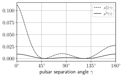
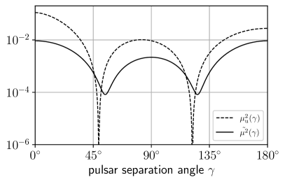
Figure 1: Comparison of $\mu_{\rm u}^{2}(\gamma)$ and $\tilde{\mu^{2}}(\gamma)$. Left panel: linear scale. Right panel: logarithmic scale, to better illustrate the regions around the two zeroes of the Hellings and Downs curve.

V Poisson distribution of sources

We have constructed ensembles in which every representative universe has exactly $N$ GW sources. However, since we do not know the correct value for $N$, we can construct a more realistic ensemble by combining these ensembles for different values of $N$. In this combination, we assume that each source has a fixed mean-squared strain $h^{2}_{0}$.

A reasonable approach is to model the possible values of $N$ as a Poisson process with a mean number of sources given by some fixed $M>0$. Thus, the ensemble contains representative universes with different values of $N$. For this Poisson model, the fraction of universes with $N$ GW sources is

$$f(N)=\frac{M^{N}}{N!}{\rm e}^{-M}\,.$$ (51)

It is easy to check that this fraction is correctly normalized, since

$$\sum_{N=0}^{\infty}f(N)=1\,.$$ (52)

The mean number of sources is

$$\langle N\rangle_{\vphantom{1^{H^{1}}}N}\equiv\sum_{N=0}^{\infty}Nf(N)=M\,.$$ (53)

This is the justification for interpreting $M$ as the mean number of GW sources in the ensemble. Also useful is the second moment

$$\langle N^{2}\rangle_{\vphantom{1^{H^{1}}}N}\equiv\sum_{N=0}^{\infty}N^{2}f(N)=M(M+1)\,.$$ (54)

Together, the first and second moments (53) and (54) imply that the variance in the expected number of sources is $\langle N^{2}\rangle_{\vphantom{1^{H^{1}}}N}-\langle N\rangle^{2}_{\vphantom{1^{H^{1}}}N}=M$. This is a standard, well known result.

V.1 Extending the discrete source ensemble to a Poisson process

One way to account for the variation in $N$ is to extend the discrete source calculation of Sec. IV. For this, we use the subscript $N$ to denote averages over the Poisson distribution of $N$, as already used in (53) and (54). The full ensemble average is

$$\langle Q\rangle=\langle Q\rangle_{{\cal A},\Omega,N}\equiv\sum_{N=0}^{\infty}f(N)\langle Q(N)\rangle_{{\cal A},\Omega}\,,$$ (55)

where $\langle Q(N)\rangle_{{\cal A},\Omega}$ denotes an ensemble average as calculated in the previous section, for an ensemble of universes containing $N$ sources.

Letting $h_{o}^{2}$ denote the mean squared strain of a single GW source, the mean of the pulsar-averaged Hellings and Downs correlation is obtained by averaging the first moment of $\Gamma(\gamma)$ given in (36). We obtain

$$\langle\Gamma(\gamma)\rangle=\langle Nh_{0}^{2}\mu_{\rm u}(\gamma)\rangle_{\vphantom{1^{H^{1}}}N}=\langle N\rangle_{\vphantom{1^{H^{1}}}N}h_{0}^{2}\mu_{\rm u}(\gamma)=Mh_{0}^{2}\mu_{\rm u}(\gamma)\,.$$ (56)

Thus, the mean-squared GW strain is the product of the expected number of sources $M$ and the expected squared GW strain $h^{2}_{0}$ of a single source.

The ensemble average of the pulsar-averaged correlation is obtained directly from (45):

$$\langle\Gamma(\gamma)\Gamma(\gamma^{\prime})\rangle \equiv\langle\Gamma(\gamma)\Gamma(\gamma^{\prime})\rangle_{{\cal A},\Omega,N}$$ (57)

$$=\langle N^{2}\rangle_{\vphantom{1^{H^{1}}}N}h_{0}^{4}\mu_{\rm u}(\gamma)\mu_{\rm u}(\gamma^{\prime})+\langle N\rangle_{\vphantom{1^{H^{1}}}N}{\mathcal{h}}_{0}^{4}\mu_{\rm u}(\gamma)\mu_{\rm u}(\gamma^{\prime})+2\bigl{(}\langle N^{2}\rangle_{\vphantom{1^{H^{1}}}N}-\langle N\rangle_{\vphantom{1^{H^{1}}}N}\bigr{)}{\mathcal{h}}_{0}^{4}\tilde{\mu^{2}}(\gamma,\gamma^{\prime})$$

$$=M(M+1)h_{0}^{4}\mu_{\rm u}(\gamma)\mu_{\rm u}(\gamma^{\prime})+M{\mathcal{h}}_{0}^{4}\mu_{\rm u}(\gamma)\mu_{\rm u}(\gamma^{\prime})+2M^{2}{\mathcal{h}}_{0}^{4}\tilde{\mu^{2}}(\gamma,\gamma^{\prime})\,.$$

Subtracting the “square” of (56) gives the cosmic covariance

$$\sigma_{\rm cos}^{2}(\gamma,\gamma^{\prime}) =\langle\Gamma(\gamma)\Gamma(\gamma^{\prime})\rangle-\langle\Gamma(\gamma)\rangle\langle\Gamma(\gamma^{\prime})\rangle$$ (58)

$$=M(h_{0}^{4}+{\mathcal{h}}_{0}^{4})\mu_{\rm u}(\gamma)\mu_{\rm u}(\gamma^{\prime})+2M^{2}{\mathcal{h}}_{0}^{4}\tilde{\mu^{2}}(\gamma,\gamma^{\prime})\,.$$

This is very similar to expression (49), which gives the cosmic covariance for exactly $N$ sources, if $N$ is replaced by the mean number $M$.

V.2 Modifying the masking function

A second (equivalent) way to employ a Poisson distribution for the number of sources is via an ensemble of masking functions, as constructed in Sec. II. In analogy with (1), we define a masking function for $N$ sources by

$$\psi(\Omega)\equiv\frac{4\pi}{M}\sum_{j=1}^{N}\delta^{2}(\Omega,\Omega_{j})\,.$$ (59)

The normalization ensures that all GW sources make the same (mean) squared-strain contribution, regardless of the value of $N$. The overall factor proportional to $1/M$ is chosen, as we will show below, to ensure that the ensemble average of $\psi$ is unity.

The construction of the ensemble of masking functions proceeds as follows. (i) Initialize the ensemble to an empty set. (ii) Fix the mean number of sources $M>0$. (iii) Select a random value of $N$ from the Poisson distribution with mean $M$ [so (51) is the probability that any particular value $N$ is obtained]. (iv) Select points $\Omega_{1},\dots,\Omega_{N}$ at random from a uniform distribution on the sphere. (v) Insert the masking function $\psi$ defined by (59) into the ensemble of masking functions. (vi) Return to step (iii).

To calculate ensemble averages involving $\psi$, we use the same methods and constructions as in Sec. II. Because (59) differs from (1) by a factor of $N/M$, the results may be obtained from those of Sec. II via a simple recipe: (A) scale each $\psi$ by a factor of $N/M$, then (B) compute the ensemble average over $N$ by means of (55).

Employing this recipe, the expected values of the spherical harmonic coefficients are obtained from (9) as follows:

$$\langle\psi_{lm}\rangle_{\vphantom{1^{H^{1}}}N}=\frac{\langle N\rangle_{\vphantom{1^{H^{1}}}N}}{M}\sqrt{4\pi}\delta_{l0}\delta_{m0}=\sqrt{4\pi}\delta_{l0}\delta_{m0}\,,$$ (60)

where the second equality follows from (53), The first moment (60) is the same as (9), implying that

$$\langle\psi(\Omega)\rangle_{\vphantom{1^{H^{1}}}N}=1\,.$$ (61)

The second moments are found from (14) by using the recipe above:

$$\langle\psi_{lm}\psi^{*}_{l^{\prime}m^{\prime}}\rangle_{\vphantom{1^{H^{1}}}N} = \frac{4\pi}{M^{2}}\Bigl{[}\langle N\rangle_{\vphantom{1^{H^{1}}}N}+\langle N^{2}-N\rangle_{\vphantom{1^{H^{1}}}N}\delta_{l0}\delta_{m0}\Bigr{]}\delta_{ll^{\prime}}\delta_{mm^{\prime}}$$ (62)

$$= {4\pi}\Bigl{[}\frac{1}{M}+\delta_{l0}\delta_{m0}\Bigr{]}\delta_{ll^{\prime}}\delta_{mm^{\prime}}\,.$$

The first equality is obtained by multiplying the final expression in (14) with $N^{2}/M^{2}$ and averaging over the Poisson distribution. The second equality follows from application of (53) and (54).

The correlation function may be obtained from (62) or directly from the final expression in (15) by employing the recipe above. It is

$$\langle\psi(\Omega)\psi(\Omega^{\prime})\rangle_{\vphantom{1^{H^{1}}}N} =\frac{4\pi}{M^{2}}\langle N\rangle_{\vphantom{1^{H^{1}}}N}\delta^{2}(\Omega,\Omega^{\prime})+\langle N^{2}-N\rangle_{\vphantom{1^{H^{1}}}N}/M^{2}$$ (63)

$$=\frac{4\pi}{M}\delta^{2}(\Omega,\Omega^{\prime})+1\,.$$

The covariance [21, Eq. (9.3)] follows immediately from (61) and (63), and is

$$C(\Omega,\Omega^{\prime}) \equiv \langle\psi(\Omega)\psi(\Omega^{\prime})\rangle_{\vphantom{1^{H^{1}}}N}-\langle\psi(\Omega)\rangle_{\vphantom{1^{H^{1}}}N}\langle\psi(\Omega^{\prime})\rangle_{\vphantom{1^{H^{1}}}N}$$ (64)

$$= \frac{4\pi}{M}\delta^{2}(\Omega,\Omega^{\prime})\,.$$

Hence, using the normalization conventions of [21, Eq. (9.4)], the covariance may be expressed as a sum of Legendre polynomials

$$C(\Omega,\Omega^{\prime})=\sum_{l=0}^{\infty}\left(\frac{2l+1}{4\pi}\right)C_{l}\,P_{l}(\Omega\cdot\Omega^{\prime})\,,$$ (65)

with coefficients $C_{l}=4\pi/M$ for all $l$. (The scale independence of these coefficients is why this is often described as a shot noise or “white” process.) This Poisson masking ensemble can be used to recover (58) via the same computation employed in (23).

VI Estimating the effects of source discreteness and galaxy clustering on the recovery of the Hellings and Downs curve

Here, we use the results of the previous sections to estimate the effects of source discreteness and galaxy clustering on the recovery of the pulsar-averaged Hellings and Downs correlation.

VI.1 Finite number of sources (shot noise)

We first consider the effects of shot noise, resulting from the discreteness of the GW sources. Simulations of the GW background produced by pairs of orbiting supermassive black holes in the centers of merging galaxies show that the signal in the PTA band is usually dominated by a handful of bright sources, of order 10 or less, see e.g., [17]. This is a tiny fraction of the ${\rm O}(10^{6})$ such systems that are contributing to the unresolved component of the GW background.

To assess the impact of the resulting shot noise, Fig. 2 compares the cosmic standard deviation of the standard Gaussian ensemble with that for $N=1$, 3, 5, 10, and 100 discrete GW sources, using (24) and (49), respectively. In the comparison, we set $h_{0}^{2}=h^{2}/N$ and ${\mathcal{h}}^{4}_{0}={\mathcal{h}}^{4}/N^{2}$ so that both ensembles have the same mean squared strain at Earth, and use $h^{2}=1$ and ${\mathcal{h}}^{2}=0.5622$, which is appropriate for a binary inspiral power spectrum for timing residual measurements (see Table 3 in [10]). The fractional increase in the standard deviation arising from GW source discreteness (shot noise) is of order $1/N$.

For $N=1$, we have $\sigma_{\rm cos}(\gamma)={\mathcal{h}}^{2}|\mu_{\rm u}(\gamma)|$, with the zeroes of the Hellings and Downs curve noticeable in the plot. For $N\lesssim 10$ discrete sources, the difference between $\sigma_{\rm cos}(\gamma)$ for the discrete-source and standard Gaussian ensemble models is $\gtrsim 10\%$, which makes a noticeable difference to the cosmic variance, particularly at small angular separations.

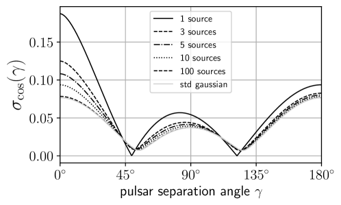
Figure 2: Comparison of the cosmic standard deviation for the standard Gaussian ensemble with that for $N=1$, 3, 5, 10, and 100 discrete sources, calculated using (24) and (49), respectively. We have matched the squared strain at Earth for the standard Gaussian ensemble and discrete source models by setting $h_{0}^{2}=h^{2}/N$ and ${\mathcal{h}}^{4}_{0}={\mathcal{h}}^{4}/N^{2}$. We have also set $h^{2}=1$ and ${\mathcal{h}}^{2}=0.5622$, which is appropriate for a binary inspiral power spectrum for timing residual measurements.

VI.2 Galaxy clustering

The matter in the universe, and galaxies in particular, are not distributed as a random Poisson process. Galaxies tend to be grouped into clusters, and these clusters form patterns of filaments and voids, known as the cosmic web. Filaments are thread-like formations where galaxies are concentrated, whereas voids are vast, relatively empty regions. This structure arises from the gravitational influence of dark matter and the universe’s initial conditions, creating a complex large-scale galaxy distribution pattern.

The length scale of the clusters is typically $\approx 10\,\text{Mpc}$, whereas the filaments and voids have $\approx 100\,\text{Mpc}$ length scales. Because the number density of galaxies is $n_{\rm G}\approx 10^{-2}\,\text{Mpc}^{-3}$ [25], these larger structures are formed from thousands or tens of thousands of galaxies. The pattern can be characterized by angular power spectra or by three-dimensional power spectra [19, 20].

However, when the universe is observed with PTAs, the effects of this structure disappear. This is because we expect that only one galaxy in every $10^{3}-10^{4}$ will host a significant PTA GW source. This means that, on the average, these PTA source host galaxies are so far apart that the effects of the clustering and structure are no longer apparent: all that remains is the effect of the point-like nature of sources, as previously estimated. Thus, the effects of galaxy clustering and the cosmic web are overwhelmed by the “shot noise” associated with the Poisson random process, exactly as we have described and calculated earlier in this paper. The amplitude of this shot noise is inversely proportional to the spatial number density of sources.

One way to see that shot noise dominates the effects of clustering is via the present-day linear-theory matter power spectrum. This can be inferred from a variety of different cosmological probes [26, Fig. 19], and is shown in Fig. 3. The actual level of power spectrum fluctuations are shown by the solid black curve, as a function of spatial frequency (wavenumber). In comparison, the dashed horizontal lines show the levels of shot noise for all galaxies [lower curve, number density $n_{\rm G}=10^{-2}(h_{100}^{-1}\,{\rm Mpc})^{-3}$] and for the small fraction of galaxies expected to host in-band PTA sources [upper curve, assumed number density $n_{\rm PTA}=3\times 10^{-6}(h_{100}^{-1}\,{\rm Mpc})^{-3}$]. The latter is more than an order-of-magnitude larger than the matter power spectrum.

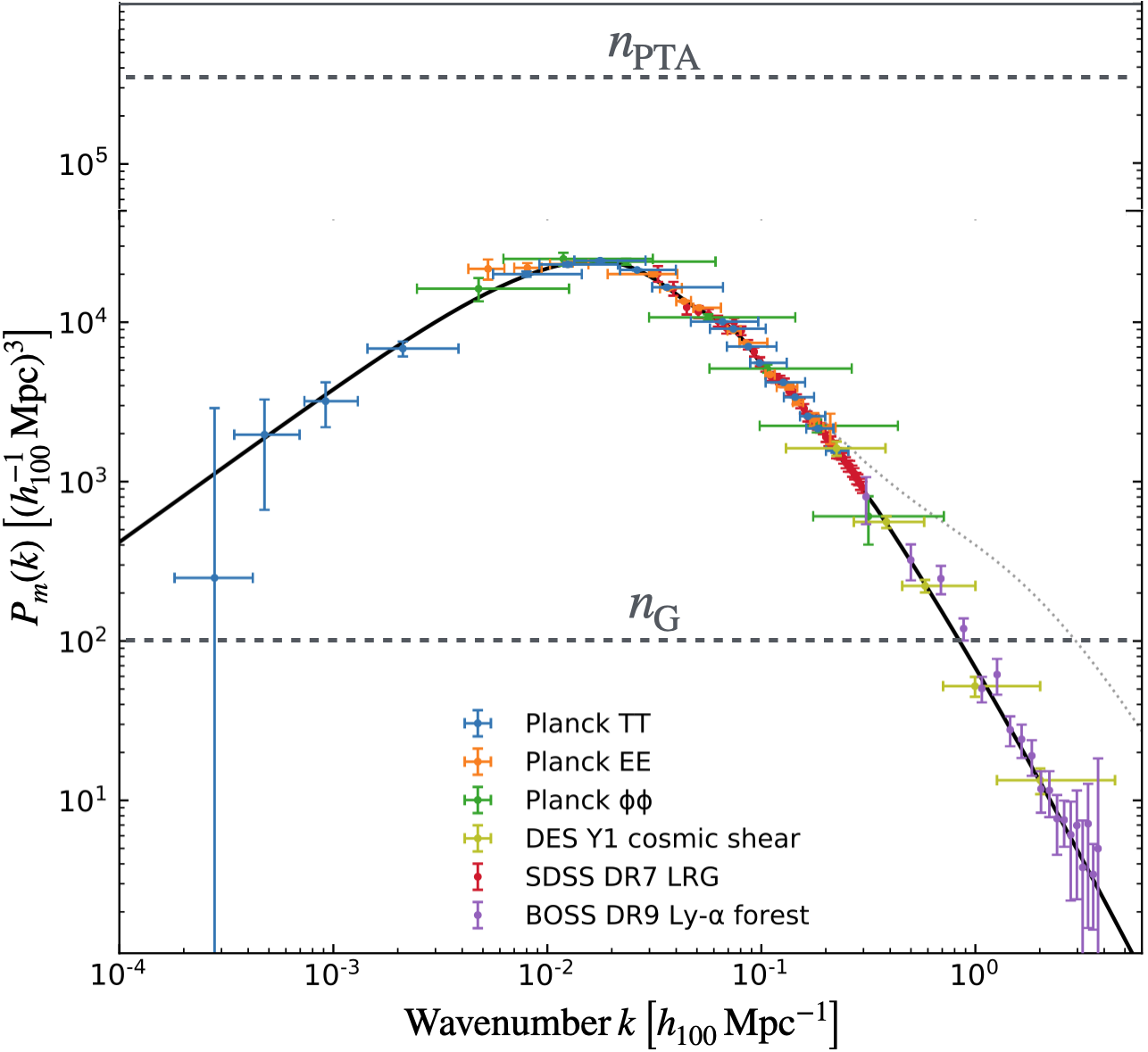
Figure 3: The solid curve shows the linear-theory matter power spectrum (at zero redshift) inferred from different cosmological probes; the dotted curve shows the impact of non-linear clustering at zero redshift. The lower horizontal dashed line is the “shot noise” power spectrum arising from the discreteness of galaxies with number density $n_{\rm G}=10^{-2}(h_{100}^{-1}\,{\rm Mpc})^{-3}$. The upper horizontal dashed line is the power spectrum of PTA GW source shot noise, assuming a number density of $n_{\rm PTA}=3\times 10^{-6}(h_{100}^{-1}\,{\rm Mpc})^{-3}$. The PTA source shot noise dominates clustering at all scales. (Plot adapted from [26, Fig. 19].)

Note that Fig. 3 shows the power spectrum of linear-theory matter density perturbations; the non-linear collapse into galaxies produces a bias that shifts the spectrum (solid curve) upwards. Typical estimates of the bias factor [27] are slightly less than 2. The upwards shift is proportional to the square of the bias factor, so these effects moves the curve upwards by less than an order of magnitude. Thus, the shot noise would always dominate.

This conclusion can be verified by using the angular correlation function of galaxies. For this purpose, we derive an upper bound on the contribution of galactic clustering to the cosmic variance, employing a simple model for the angular power spectrum,

$$C_{L}=\begin{cases}C_{0}&{\rm for}\quad L\leq L_{\rm max}\\ 0&{\rm for}\quad L>L_{\rm max}\,.\end{cases}$$ (66)

To obtain an upper bound, start with the expression for the cosmic variance in terms of the angular power spectrum, see (9.10) and (9.4) in [21]:

$$\sigma^{2}_{\rm cos}(\gamma)=2{\mathcal{h}}^{4}\tilde{\mu^{2}}(\gamma)+\frac{C_{0}}{4\pi}h^{4}\mu_{u}^{2}(\gamma)+\frac{1}{2}{\mathcal{h}}^{4}\int_{0}^{\pi}{\rm d}(\cos\beta)\sum_{L=0}^{\infty}\left(\frac{2L+1}{4\pi}\right)C_{L}P_{L}(\cos\beta)\left[\mu^{2}(\gamma,\beta)+\mu^{2}(\bar{\gamma},\bar{\beta})\right]\,.$$ (67)

Begin by assuming that $C_{L}=C_{0}$ for all $L$, so out to $L_{\rm max}=\infty$. Then the summation in (67) is easy to do since

$$\sum_{L=0}^{\infty}\Bigl{(}\frac{2L+1}{2}\Bigr{)}P_{L}(\cos\beta)=\delta(\cos\beta-1)\,,$$ (68)

which can be obtained from Eq. (4.2) of [21] by setting $x=\cos\beta$ and $x^{\prime}=1$. The integral over $\cos\beta$ is trivial, so the third term on the rhs of (67) simplifies to

$${\rm third\ term}=\frac{1}{4\pi}{\mathcal{h}}^{4}C_{0}\mu_{\rm u}^{2}(\gamma)\,,$$ (69)

where we used $\mu^{2}(\gamma,0)=\mu_{\rm u}^{2}(\gamma)$ and $\mu^{2}(\bar{\gamma},\pi)=0$.

Expression (69) for the third term of (67) implies an upper bound on the cosmic variance for the $C_{L}$ given in (66). This is because any single $C_{L}>0$ makes a contribution to the cosmic variance which is necessarily non-negative. A proof by contradiction follows. Suppose that for some $L$ value

$$\frac{1}{2}{\mathcal{h}}^{4}\int_{0}^{\pi}{\rm d}(\cos\beta)\left(\frac{2L+1}{4\pi}\right)P_{L}(\cos\beta)\left[\mu^{2}(\gamma,\beta)+\mu^{2}(\bar{\gamma},\bar{\beta})\right]<0\,.$$ (70)

Then, by choosing that $C_{L}$ to be large enough to dominate the first two terms in (67), we could make $\sigma^{2}_{\rm cos}(\gamma)<0$. This is a contradiction, since by definition $\sigma^{2}\geq 0$.

So, we have proven that for the $C_{L}$ model given in (66)

$$\sigma^{2}_{\rm cos}(\gamma)\leq 2{\mathcal{h}}^{4}\tilde{\mu^{2}}(\gamma)+\frac{1}{4\pi}(h^{4}+{\mathcal{h}}^{4})C_{0}\mu_{\rm u}^{2}(\gamma)\,.$$ (71)

If we now use

$$C_{0}=0.002\,,\qquad L_{\rm max}=50\,,$$ (72)

to describe the effects of galaxy clustering [20] the contribution of these $C_{L}$’s to the cosmic variance is less than one percent of that for the standard Gaussian ensemble. Thus, galaxy clustering does not make a significant contribution to the cosmic variance of the pulsar-averaged Hellings and Downs correlation. This is consistent with the results of [22, Fig. 2] for these small values of $C_{0}$.

VII Conclusion

This paper uses the general method developed in [21, 22] to assess the effects of (a) source discreteness and (b) galaxy clustering on the Hellings and Downs correlation. The impact is measured by comparing the cosmic variance of the pulsar-averaged correlation $\Gamma$ in the standard Gaussian ensemble to the same quantity in an ensemble which models (a) or (b). Here, $\Gamma$ quantifies “how closely” the Hellings and Downs correlation is expected to approach the Hellings and Downs curve. This provides an order-of-magnitude estimate of the impact of these effects.

For (a) we compared ensembles containing a Poisson distribution of $N$ discrete sources to the Gaussian ensemble. The latter corresponds to a very large number of very weak sources. We found (see Fig. 2) that for typical numbers of strong PTA sources $N\approx 10$ this shot noise effect increases the cosmic standard deviation of the pulsar-averaged Hellings and Downs correlation by an amount $1/N\approx 10\%$. For (b) we compared the Gaussian ensemble without source correlations to an ensemble with typical galactic structure correlations. Here, the effects are very small, less than 1%, and completely dominated by the shot noise contributions (a) [see Fig.  3 and text following (72)]. These results provide a useful quantitative test and point of comparison for more authentic computer simulations.

This work could be usefully extended by modifying the statistical ensembles to make them more realistic. We do not expect that this will change the order-of-magnitudes of the different effects, but it might be helpful to quantify this.

Our model (ensemble) of $N$ discrete GW sources assumes that these have a Gaussian distribution of amplitudes, drawn from a power spectrum. Physically, this corresponds to picking $N$ lines of sight (directions on the sphere). Then, for each of these sky directions, a large number of of independently radiating GW sources are stacked up “on top of each other” along that line of sight. For each direction, enough sources are stacked that the central limit theorem applies, and the resulting GW amplitudes along each of the $N$ directions has the same Gaussian distribution.

These calculations could be improved by using a more realistic ensemble. For this, along each of the $N$ directions, there would be one GW source, which radiates at a single frequency with a specific (but unknown) phase and polarization. Rather than selecting the amplitudes from the same distributions, one could use distributions whose mean squared amplitudes are largest for the “closest” source and are smaller for more distant ones. Such calculations are not difficult to carry out, and appear to give results similar to those presented here.

References

• Antoniadis et al. [2023] J. Antoniadis et al. (EPTA and InPTA Collaborations), The second data release from the European Pulsar Timing Array: III. Search for gravitational wave signals, Astronomy $\&$ Astrophysics 678, A50 (2023).
• Agazie et al. [2023] G. Agazie et al. (NANOGrav Collaboration), The NANOGrav 15 yr Data Set: Evidence for a Gravitational-wave Background, The Astrophysical Journal Letters 951, L8 (2023).
• Reardon et al. [2023] D. J. Reardon et al. (PPTA Collaboration), Search for an Isotropic Gravitational-wave Background with the Parkes Pulsar Timing Array, The Astrophysical Journal Letters 951, L6 (2023).
• Xu et al. [2023] H. Xu et al. (CPTA Collaboration), Searching for the Nano-Hertz Stochastic Gravitational Wave Background with the Chinese Pulsar Timing Array Data Release I, Research in Astronomy and Astrophysics 23, 075024 (2023).
• Allen and Romano [1999] B. Allen and J. D. Romano, Detecting a stochastic background of gravitational radiation: Signal processing strategies and sensitivities, Phys. Rev. D 59, 102001 (1999).
• Chamberlin et al. [2015] S. J. Chamberlin, J. D. E. Creighton, X. Siemens, P. Demorest, J. Ellis, L. R. Price, and J. D. Romano, Time-domain implementation of the optimal cross-correlation statistic for stochastic gravitational-wave background searches in pulsar timing data, Phys. Rev. D 91, 044048 (2015).
• Romano and Cornish [2017] J. D. Romano and N. J. Cornish, Detection methods for stochastic gravitational-wave backgrounds: a unified treatment, Living Rev. Relativ. 20, 2 (2017).
• Ellis et al. [2020] J. Ellis, M. Vallisneri, S. Taylor, and P. Baker, ENTERPRISE: Enhanced Numerical Toolbox Enabling a Robust PulsaR Inference SuitE, Zenodo 10.5281/zenodo.4059815 (2020).
• Romano et al. [2021] J. D. Romano, J. S. Hazboun, X. Siemens, and A. M. Archibald, Common-spectrum process versus cross-correlation for gravitational-wave searches using pulsar timing arrays, Phys. Rev. D 103, 063027 (2021).
• Allen and Romano [2023] B. Allen and J. D. Romano, Hellings and Downs correlation of an arbitrary set of pulsars, Phys. Rev. D 108, 043026 (2023).
• Romano and Allen [2024] J. D. Romano and B. Allen, Answers to frequently asked questions about the pulsar timing array Hellings and Downs curve (2024), arXiv:2308.05847 [gr-qc] .
• Allen [2023] B. Allen, Variance of the Hellings-Downs correlation, PRD 107, 043018 (2023).
• Allen and Valtolina [2024] B. Allen and S. Valtolina, Pulsar timing array source ensembles, Phys. Rev. D 109, 083038 (2024).
• Cornish and Sesana [2013] N. J. Cornish and A. Sesana, Pulsar timing array analysis for black hole backgrounds, Classical and Quantum Gravity 30, 224005 (2013).
• Cornish and Sampson [2016] N. J. Cornish and L. Sampson, Towards robust gravitational wave detection with pulsar timing arrays, Physical Review D 9310.1103/physrevd.93.104047 (2016).
• Bécsy and Cornish [2020] B. Bécsy and N. J. Cornish, Joint search for isolated sources and an unresolved confusion background in pulsar timing array data, Classical and Quantum Gravity 37, 135011 (2020).
• Bécsy et al. [2022] B. Bécsy, N. J. Cornish, and L. Z. Kelley, Exploring realistic nanohertz gravitational-wave backgrounds, The Astrophysical Journal 941, 119 (2022).
• Agazie et al. [2024] G. Agazie et al. (NANOGrav Collaboration), The NANOGrav 15 yr Data Set: Looking for Signs of Discreteness in the Gravitational-wave Background (2024), arXiv:2404.07020 .
• Frith et al. [2005] W. J. Frith, P. J. Outram, and T. Shanks, The 2-Micron All-Sky Survey galaxy angular power spectrum: probing the galaxy distribution to gigaparsec scales, Monthly Notices of the Royal Astronomical Society 364, 593 (2005).
• Ando et al. [2017] S. Ando, A. Benoit-Lévy, and E. Komatsu, Angular power spectrum of galaxies in the 2MASS Redshift Survey, Monthly Notices of the Royal Astronomical Society 473, 4318 (2017).
• Allen [2024] B. Allen, Pulsar timing array harmonic analysis and source angular correlations, arXiv:2404.05677 (2024), arXiv:2404.05677 [gr-qc] .
• Agarwal and Romano [2024] D. Agarwal and J. D. Romano, Cosmic variance of the Hellings and Downs correlation for ensembles of universes having non-zero angular power spectra (2024), arXiv:2404.08574 [gr-qc] .
• Grimm et al. [2024] N. Grimm, M. Pijnenburg, G. Cusin, and C. Bonvin, The impact of large-scale galaxy clustering on the variance of the Hellings-Downs correlation (2024), arXiv:2404.05670 [astro-ph.CO] .
• Isserlis [1918] L. Isserlis, On a formula for the product-moment coefficient of any order of a normal frequency distribution in any number of variables, Biometrika 12, 134 (1918), note that Isserlis’ theorem is often called “Wick’s theorem” in the physics community, although the Wick’s work was three decades later.
• Conselice et al. [2016] C. J. Conselice, A. Wilkinson, K. Duncan, and A. Mortlock, The evolution of galaxy number density at $z<8$ and its implications, The Astrophysical Journal 830, 83 (2016).
• Aghanim, N. et al. [2020] Aghanim, N. et al. (Planck Collaboration), Planck 2018 results - I. Overview and the cosmological legacy of Planck, A&A 641, A1 (2020).
• Einasto et al. [2019] J. Einasto, L. J. Liivamägi, I. Suhhonenko, and M. Einasto, The biasing phenomenon, Astronomy and Astrophysics 630, A62 (2019).