Considerations about the measurement of the magnetic moment and electric dipole moment of the electron

Abstract

The goal of the measurement of the magnetic moment of the electron $\boldsymbol{\mu}$, is to experimentaly determine the gyromagnetic ratio. The factor $g/2$ is computed by the accurate measurement of two frequencies, the spin precession frequency $\nu_{s}$, and the cyclotron frequency $\nu_{c}$, and is defined as $\nu_{s}/\nu_{c}=g/2$. These experiments are performed with a single electron confined inside a Penning trap. The existence of the electric dipole moment ${\bi d}_{e}$, involves the idea of an asymmetric charge distribution along the spin direction such that ${\bi d}_{e}=d_{e}{\bi S}/(\hbar/2)$. The energy shift $\Delta U=2{d}_{e}E_{eff}$ of the interaction of the electric dipole of electrons with a huge effective electric field ${\bi E}_{eff}$, close to the nucleus of heavy neutral atoms or molecules, is determined by a spin precession measurement. By using a classical model of a spinning electron, which satisfies Dirac’s equation when quantized, we determine classically the time average value of the electric and magnetic dipole moments of this electron model when moving in a uniform magnetic field and in a Penning trap, with the same fields as in the real experiments, and obtain an estimated value of these dipoles. We compare these results with the experimental data and make some interpretation of the measured dipoles.

Keywords: Spinning electron; gyromagnetic ratio; electric dipole moment

1 Introduction

In the analysis of the electron structure, Dirac [1] found to first order in the external electromagnetic field, two interacting terms $-{\bi d}{\cdot}{\bi E}-{\boldsymbol{\mu}}{\cdot}{\bi B}$, which he interpreted as if the electron behave as though it has a magnetic moment $\boldsymbol{\mu}$ and an electric dipole moment ${\bi d}$. This magnetic moment is just that assumed in the spinning electron model. Dirac disliked the existence of the electric dipole, perhaps considering that it was related to some asymmetry of the spherical charge distribution of the electron. In his words it is doubtful whether the electric moment has a physical meaning. Two years later, when published his book [2], there was no single mention to this electric dipole moment.

The predicted magnetic moment $\mu_{B}=e\hbar/2m$, called Bohr’s magneton, was the expected magnetic moment which justified Zeeman’s effect and the hyperfine structure of the hydrogen atom, and it was one of the greatest predictions and success of Dirac’s theory. Preliminary measurements of the magnetic moment show that its value is different than the predicted one $\mu=(g/2)\mu_{B}$, where the coefficient $g\neq 2$, is called the gyromagnetic ratio, and is considered an intrinsic property of the electron. Since then, theoretical and experimental physicists have considered also the possibility of the existence of the predicted electric dipole moment, and very challenging experiments have been designed for the measurement of both properties.

For the measurement of the magnetic moment the challenge has been to isolate a single electron in a cavity, under external electric and magnetic fields, and to monitorize its excited states to determine this property. We shall describe in section 2 one of these Penning traps. In section 3 we describe the motion of a spinless point particle in this cavity to show its expected motion. Because it is a spinless model we cannot describe the motion of the spin, which is going to be relevant for the determination, at least, of the magnetic moment orientation. The next two sections 4 and 5 are a summary of the experimental setups for the measurements of both dipoles.

Section 6 is devoted to a summary of a classical description of a spinning electron, which has been obtained from a general formalism for describing classical elementary spinning particles [3]. One of the main features is that the electron is described by the evolution of a single point ${\bi r}$, considered as the center of charge, which satisfies a system of fourth-order differential equations. Its trajectory has curvature and torsion, and therefore its classical hellical trajectory suggests the so called zitterbewegung motion. The center of mass is a different point than the center of charge, and it is defined in terms of the point ${\bi r}$ and their derivatives. The center of mass is some average of the position of the evolution of the center of charge. In this section it is also analyzed the motion of the spinning particle in a uniform magnetic field to determine that the spin precess backwards with the angular velocity $\omega_{s}=-\omega_{c}/2$, where $\omega_{c}=eB/m$, is the cyclotronic angular velocity. We end this section with a classical relativistic definition of the electric dipole moment and magnetic moment for a spinning particle, suggested by the previous classical structure. The definition of the magnetic moment of a spinning particle is different than for the spinless point particle. If we accept that this model is a classical description of the electron, then is the relative motion of the center of charge around the center of mass which produces the magnetic moment. The existence of the electric dipole moment is not related to any asymmetry in the charge distribution. It is related to the separation between the center of mass and center of charge.

In section 7 we analyse the motion of the Dirac particle in the Penning trap and obtain an estimation for the time average values of the magnetic moment and electric dipole moment. We end with some conclusions at section 8.

2 The Penning trap. The Geonium

The Penning trap is a cylindrical cavity, like the one depicted in the figure 1. It is bounded by a positively charged one-sheet hyperboloid and two caps, that have the shape of a negatively charged two-sheet hyperboloid. Inside, a vacuum has been created, it is cooled to a very low temperature and there is also a magnetic field in the axial direction.

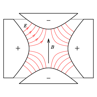
Figure 1: Model of a Penning trap where an electrostatic field between the positively charged lateral wall, and the two negatively charged caps, is established. Superimposed there is also a uniform axial magnetic field. Red lines correspond to the field lines of the electrostatic field.

If electrons are injected into the cavity, they begin to rotate due to the magnetic field. If they have an initial velocity along the magnetic field, when they approach to the negatively charged caps, they will be repelled and therefore the electrons are trapped inside the cavity. The walls of the cavity are equipotential surfaces of the electrostatic potential. The electrostatic potential, in cylindrical coordinates, has the form

$$V(z,r)=V_{0}\frac{r^{2}-2z^{2}}{4d^{2}},\quad\nabla^{2}V=0.$$

It satisfies Laplace’s equation in the cavity. The surfaces $2z^{2}-r^{2}=$ const. are equipotential surfaces. If this constant is positive, the origin of the reference system is at the center of the device and the vertex of each cap is at the position $(0,0,\pm z_{0})$, the equation of the two-sheeted hyperboloid corresponding to the caps, in Cartesian coordinates, is

$$z^{2}=z_{0}^{2}+(x^{2}+y^{2})/2.$$

The surfaces $2z^{2}-r^{2}=$ cte $<0$, are also equipotential surfaces. If $r_{0}$ is the radius of the throat of the one-sheeted lateral wall, the equation of this hyperboloid is

$$z^{2}=\frac{1}{2}(x^{2}+y^{2}-r_{0}^{2}).$$

The equipotential surface $2z^{2}-r^{2}=0$, is the cone, centered at the origin, whose generatrices define the asymptotic directions of the two hyperboloids and of the equipotential surfaces of the electrostatic field. Therefore,

$$V(z_{0},0)-V(0,r_{0})=-\frac{V_{0}z_{0}^{2}}{2d^{2}}-\frac{V_{0}r_{0}^{2}}{4d^{2}},$$

and if we choose for the parameter $d$, the value

$$d^{2}=\frac{1}{2}(z_{0}^{2}+r_{0}^{2}/2),\quad V(z_{0},0)-V(0,r_{0})=-V_{0}<0,$$

then $V_{0}$, is the difference of the electrostatic potential between the two hyperboloids, being positive the lateral one-sheeted hyperboloid (as shown in the figure 1).

We take for the vector potential of the uniform magnetic field ${\bi B}$,

$${\bi A}=\frac{1}{2}{\bi B}\times{\bi r}=\frac{1}{2}Br\widehat{\bi e}_{\phi},\quad\nabla\times{\bi A}={\bi B}=B\widehat{\bi e}_{z}.$$

The Lagrangian which describes the electron in this cavity is:

$${L}={L}_{0}-eV+e\dot{\bi r}\cdot{\bi A},\quad\dot{\bi r}\cdot{\bi A}=\frac{1}{2}{\bi B}\cdot({\bi r}\times\dot{\bi r}),$$

where ${\bi r}$ and $\dot{\bi r}$, are, respectively, the position and velocity of the center of charge of the electron in the laboratory reference system, and ${L}_{0}$ is the free Lagrangian. In Cartesian coordinates it appears as:

$$L=L_{0}-eV_{0}\frac{2z^{2}-(x^{2}+y^{2})}{4d^{2}}+\frac{eB}{2}(x\dot{y}-y\dot{x}),$$

where the overdot means to take the time derivative.

3 Non-relativistic spinless point particle

In the non-relativistic framework and for the spinless point particle, the center of charge and center of mass of the electron are the same point and the free Lagrangian $L_{0}$, is

$$L_{0}=\frac{m}{2}\left(\dot{x}^{2}+\dot{y}^{2}+\dot{z}^{2}\right).$$

The Lagrangian can be written in two parts, one a function of only $z$ and $\dot{z}$, and another which depends on the variables $x,y,\dot{x},\dot{y}$,

$$L=L_{1}(z,\dot{z})+L_{2}(x,y,\dot{x},\dot{y}),$$

where

$$L_{1}(z,\dot{z})=\frac{m}{2}\dot{z}^{2}-\frac{eV_{0}}{2d^{2}}z^{2},$$

$$L_{2}(x,y,\dot{x},\dot{y})=\frac{m}{2}(\dot{x}^{2}+\dot{y}^{2})+\frac{eV_{0}}{4d^{2}}(x^{2}+y^{2})+\frac{eB}{2}(x\dot{y}-y\dot{x}).$$

The dynamical equation corresponding to the $z$ variable is decoupled with the other two and it turns out to be

$$m\ddot{z}+\frac{eV_{0}}{d^{2}}z=0,\quad\ddot{z}+\omega_{z}^{2}z=0,\quad\omega_{z}^{2}=\frac{eV_{0}}{md^{2}}>0,$$

since for the electron $e<0$ and in the cavity we take $V_{0}<0$. It represents a vertical harmonic oscillation of constant pulsation $\omega_{z}$. When quantizing this model, there will be a quantized harmonic energy of value $H_{z}=\hbar\omega_{z}(n_{z}+1/2)$, where $n_{z}$ represents the number of quanta of this mode. The variables $x$ and $y$, satisfy the equations

$$\ddot{x}+\omega_{c}\dot{y}-\frac{1}{2}\omega_{z}^{2}x=0,\quad\ddot{y}-\omega_{c}\dot{x}-\frac{1}{2}\omega_{z}^{2}y=0,\quad\omega_{c}=\frac{eB}{m}.$$

If $\omega_{z}=0$, we obtain a circular motion perpendicular to the magnetic field, with cyclotronic angular velocity $\omega_{c}$. The presence of the last term, which depends on $\omega_{z}^{2}$, is the radial atracting force of the lateral wall. If we use a dimensionless time evolution parameter $\widetilde{t}=\omega_{c}t$, the equations of the point particle in the cavity are the linear equations:

$$\ddot{x}=-\dot{y}+\frac{a}{2}x,\quad\ddot{y}=\dot{x}+\frac{a}{2}y,\quad\ddot{z}=-az,\quad a=\frac{\omega_{z}^{2}}{\omega_{c}^{2}},$$ (1)

depending on a single dimensionless parameter $a$, and where the overdot represents the derivative with respect to the dimensionless time $\widetilde{t}$. The centrifugal acceleration is radial, and the rotation angular velocity is unity along $OZ$ axis. The result is that a kind of epicyclic motion of angular velocity $\omega_{m}\approx\omega_{z}^{2}/\omega_{c}$, is superimposed on the cyclotronic motion of angular velocity $\omega_{c}$, and a harmonic motion of pulsation $\omega_{z}$ in the vertical direction. A possible trajectory of a spinless electron is that of the figure 2, for $a=0.001$. It depends crucially on the initial $z(0)$ location, because the vertical oscillation is in the range $(-z(0),z(0))$, with an almost circular horizontal motion on the XOY plane.

These three frequencies

$$\omega_{m}=2\pi\nu_{m}\simeq\frac{\omega_{z}^{2}}{2\omega_{c}}=\frac{V_{0}}{2Bd^{2}},\quad\omega_{z}=2\pi\nu_{z}=\sqrt{\frac{eV_{0}}{md^{2}}},\quad\omega_{c}=2\pi\nu_{c}=\frac{eB}{m},$$

are independent of the velocity of the electron, but they depend on the external fields. The magnetronic pulsation $\omega_{m}$, is independent of the kind of the particle, and only depends on the static fields and the dimensions of the Penning trap. The dimensionless parameter $a$, is:

$$a=\frac{m}{e}\frac{V_{0}}{B^{2}d^{2}}.$$

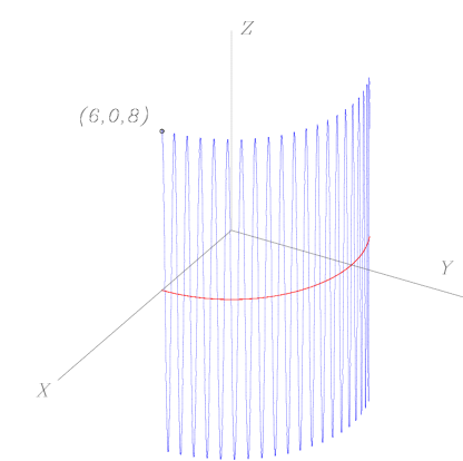
Figure 2: Motion of the spinless point particle (blue), with initial position in $(x_{0},y_{0},z_{0})=(6,0,8)$, initial velocity $(u_{x},u_{y},u_{z})=(0,0.0001,0)$, and where the parameter $a=0.001$. It is also depicted the projection of the motion (red) on the $XOY$ plane.

A typical cavity, the one built by Gabrielse and Dehmelt [4], has the dimensions and fields $d=z_{0}=r_{0}/\sqrt{2}=0.335$ cm, $V_{0}=10.22$ V, $B=5.872$ T. With these data, the motion of the electron is a superposition of different harmonic motions, of pulsations:

$$\omega_{m}=7.7543\cdot 10^{4}\,{\rm s}^{-1},\quad\omega_{z}=4.0021\cdot 10^{8}\,{\rm s}^{-1},\quad\omega_{c}=1.0327\cdot 10^{12}\,{\rm s}^{-1}.$$

The quanta of these modes are of energies:

$$\hbar\omega_{m}=5.104\cdot 10^{-11}{\rm eV},\quad\hbar\omega_{z}=2.634\cdot 10^{-7}{\rm eV},\quad\hbar\omega_{c}=6.797\cdot 10^{-4}{\rm eV},$$

and frequencies

$$\nu_{m}=12.3414\,{\rm kHz},\quad\nu_{z}=63.6956\,{\rm MHz},\quad\nu_{c}=164.37047\,{\rm GHz}.$$

The value of the parameter $a=1.5016\cdot 10^{-7}$. In a Penning trap we get that, in general, $\nu_{m}\ll\nu_{z}\ll\nu_{c}$.

The electrons, trapped in this cavity, undergone transitions by quanta of the above energies. The quantum excited states are represented as $|n_{c},n_{z},n_{m}>$, where $n_{i}$, $i=c,z,m$, are the number of the quanta of each mode. When the energy increases, electrons move faster, the radius increases and some electrons can reach the side walls of the cavity and be absorbed by the metallic structure. The energy radiated by the electrons is monitored and every time an electron dissapears, there is a sudden decrease in the radiated energy. When in the end, the radiated signal corresponds to a single electron, experimentalists conclude that the cavity contains a single electron bound to the Earth. The authors give the name of Geonium to this single electron captured in a Penning trap. The experimental challenge has been to succesfully monitor these excited quantum states of Geonium.

The different order of magnitude of these frequencies $\nu_{c}$, $\nu_{z}$ and $\nu_{m}$, suggests that the fundamental experimental role will is played by the accurate measurement of the frequency $\nu_{c}$, and to the next order $\nu_{z}$.

In the cavity, the ground state of the electron corresponds to $|0,0,0>$. With the above fields, the energy of this state is

$$H_{0}=\gamma(v)mc^{2}=mc^{2}+\hbar(\omega_{c}+\omega_{z}+\omega_{m})/2>mc^{2},$$

and the velocity of the electron is

$$\gamma(v)=1.000000000665396,\quad v/c=0.00003648,\quad v=10936.4\,{\rm m/s}.$$

In a nonrelativistic analysis we obtain the same value

$$\frac{1}{2}mv^{2}=\hbar(\omega_{c}+\omega_{z}+\omega_{m})/2,\quad v=10936.4\,{\rm m/s}.$$

The electron, even at its lowest energy state, is never at rest. With this velocity in the Penning trap, the cyclotron radius is

$$R_{c}=v/\omega_{c}=1.05901\cdot 10^{-8}\;{\rm m}.$$

This linear relation means that the cyclotronic radius increases with the electron velocity.

4 Experimental measurement of $g$

We are going to summarize basic aspects of the experiments of the following three works: The oldest one from 1986, which we will call (W) for Washington [5], and whose main conclusions were presented in the Letter [6]; the most recent one of 2023, we are going to call (N) for Northwestern [7], that makes a comparison of its results with an intermediate one from 2008, called (H) for Harvard [8]. These symbols make reference to the universities where these experiments took place.

The experimental challenge is to isolate a single electron in a Penning trap at very low temperature, interact and excite the electron, produce different transitions and measure the aforementioned frequencies of the different modes. The goal of these experiments is to accurately measure the cyclotronic angular velocity $\omega_{c}$, and the spin precession angular velocity $\omega_{s}$.

The hypothesis of these works is that the different energy levels of this single electron in the cavity are quantized according to

$$H=H_{s}+H_{c}=\hbar\omega_{s}m_{s}+\hbar\omega_{c}\left(n+\frac{1}{2}\right),$$

where $m_{s}=\pm 1/2$, and $n$ represents the number of excited quanta of the cyclotronic motion of angular velocity $\omega_{c}=eB/m$. The other modes $\omega_{m}$ and $\omega_{z}$, are considered not very relevant.

We know that if a spinning particle in a uniform magnetic field describes a cyclotron trajectory of angular velocity $\omega_{c}$, the spin precess backwards with the angular velocity $-\omega_{c}/2$. In these experimental works they assume that the spin precession angular velocity is $g$ times this value, $\omega_{s}=g\omega_{c}/2$. In this way $\omega_{s}/\omega_{c}=g/2$, and the accurate measurement of these two frequencies will give the value of $g$:

$$\frac{g}{2}=\frac{\omega_{s}}{\omega_{c}}=1+\frac{\omega_{s}-\omega_{c}}{\omega_{c}}=1+\frac{\omega_{a}}{\omega_{c}},\quad\omega_{a}=\omega_{s}-\omega_{c}.$$

In (N) they denominate $\nu_{a}=\omega_{a}/2\pi$, the anomaly frequency, and the measurement of $\nu_{a}/\nu_{c}$ rather than $\nu_{s}/\nu_{c}$, significantly reduces the effect of frequency measurement uncertainties, in their words. For example, they mention, that in a magnetic field of $B=5.3$ T, they obtain the following approximate values: $\nu_{c}=\omega_{c}/2\pi\approx$149 GHz, $\nu_{a}=\omega_{a}/2\pi\approx$173 MHz. This gives the value

$$\frac{g}{2}=1.001161073825504,$$

which is a good aproximation to the expected gyromagnetic ratio. What they do is to take a sufficient number of measurements of these frequencies, under different magnetic fields, and take the corresponding statistical average. In the figure 4 of the cited (N) paper they mention that they have done 11 measurements with different values of the magnetic field $B$, in the range of 3 to 5.5 Teslas.

As a summary of these works the following measurements of $g/2$, have been obtained:

$$1986\quad(W)\quad{g}/{2} = 1{\rm.}001\,159\,652\,200\,(40),$$ (2)

$$2008\quad(H)\quad{g}/{2} = 1{\rm.}001\,159\,652\,180\,73\,(28),$$ (3)

$$2023\quad(N)\quad{g}/{2} = 1{\rm.}001\,159\,652\,180\,59\,(13).$$

In this last measurement (N), they ensure that it is 2.2 times more accurate than in (H), from the statistical point of view.

In the Van Dyck et al. work (W) the Penning trap is something different as the one described above, with an electrostatic potential

$$V(z,r)=V_{0}\frac{r^{2}-2z^{2}}{4d^{2}}+V_{0}C_{4}\frac{8z^{4}-24r^{2}z^{2}+3r^{4}}{16d^{4}},$$

where the coefficient $C_{4}$ depends on the geometry of the cavity. It is cooled to 4 K and a magnetic field of 1.8 T is used. In the other two works (N) and (H) the authors mention that the Penning trap is cylindrical. In (N) the cavity is cooled up to 50 mK, with the surrounding solenoid cooled at 4.2 K and the magnetic field range is from 3 to 5.5 T.

5 Experimental measurement of the Electric dipole moment

We are going to analyze a recent experiment [9], to measure the electric dipole moment of the electron. The experimental setup consists of sending a beam of neutral heavy atoms or molecules, in this case thorium monoxide (ThO), between two charged plates, parallel to the XOY plane, separated 25 mm. There is a uniform electric $E_{z}$, and a uniform magnetic field $B_{z}$, orthogonal to the plates, as depicted in figure 3. The use of heavy atoms is because the effective electric field $E_{eff}$, at points very close to the nucleus is around $10^{6}$ times stronger than any electric field produced at the laboratory. If the electrons have an electric dipole ${\bi d}_{e}$, in its ground state it will be oriented along the efective electric field, so that the energy of this state is $-d_{e}E_{eff}$. If we excite the molecules by a transversal optical pumping at the area $A$, some electrons will jump to the excited state with the dipole orientation reversed, after the absortion of energy of order $\Delta U=2d_{e}E_{eff}$. This energy will be determined in the detection area $D$, by measuring the energy of the emited photons of this spontaneous emission.

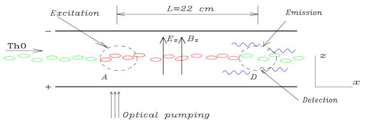
Figure 3: Evolution of the ThO molecules inside the cavity. In the region $A$ some molecules are excited (green to red) the corresponding excited electron reverses its electric dipole orientation by absorbing some photons of the optical pumping. Later, the molecule makes a spontaneous emission at the region $D$, where detectors are located, and the energy of emited photons is measured.

The main theoretical assumption is that the electric dipole has the same orientation as the spin ${\bi d}_{e}=d_{e}{\bi S}/(\hbar/2)$, and if the molecules interact with the external field $B_{z}$, the spin precession will also be the electric dipole precession. During the time of flight of the molecules, the magnetic moment of the excited electron of value $(g/2)\mu_{B}$, interacts with the external magnetic field $B_{z}$, and the spin will precess an angle $\phi$, in the $XOY$ plane, which is the same precession angle of the electric dipole. This precession angle is going to be measured at the readout section $D$ of the experiment, where the fluorescence detectors are located.

The experimental hypothesis is that this precession angle of the spin is

$$\phi\approx\left(-g\mu_{B}B_{z}-d_{e}E_{eff}\right)\tau/\hbar,$$ (4)

where $\tau\approx 1.1$ ms, is the time of flight of the molecules between the excitation area $A$ and detection area $D$, which are separated by a distance $L\approx 22$ cm. If $\phi$ and $\Delta U$, are accurately measured, they determine the values of $d_{e}$ and $E_{eff}$.

The experimental result suggests that the upper bound for the electric dipole is

$$d_{e}<8.7\cdot 10^{-29}\,e\,{\rm cm}.$$

6 Classical Dirac particle

The model of a classical elementary spinning particle that we are going to use in this work, has been obtained through a general formalism [3], that is based on the following three fundamental principles: Restricted Relativity Principle, Variational Principle and Atomic Principle.

The definition of a classical elementary particle lies on the Atomic principle [10]. The idea is that an elementary particle does not have internal excited states in the sense that any interaction, if it does not annihilate the particle, does not modify its internal structure. If an inertial observer describes the state of the elementary particle through a set of variables $(x_{1},\ldots,x_{n})$ and the dynamics changes this state to another $(y_{1},\ldots,y_{n})$, if the internal structure has not been modified, then it is possible to find another inertial observer who describes this new state of the particle with exactly the same values of the variables of the previous state. This means that there must be a Poincaré transformation $g$, between both inertial observers in such a way that the above values are transformed into each other:

$$(y_{1},\ldots,y_{n})=g\,(x_{1},\ldots,x_{n}).$$

This relation must be valid for any pair of states of any elementary particle. The Atomic Principle restricts the classical variables of the variational description of an elementary particle, to span a homogeneous space of the Poincaré group [3]. Then the initial and final states of the Lagrangian description are described by as many variables as those of any Poincaré group element, and with the same geometrical or physical meaning like the group parameters. The initial state is characterized by the variables $x_{i}\equiv(t,{\bi r},{\bi u},\boldsymbol{\alpha})$, that are interpreted as the time $t$, the position of a single point ${\bi r}$, the velocity of this point ${\bi u}$, and finally the orientation $\boldsymbol{\alpha}$ of a comoving Cartesian frame attached to the point ${\bi r}$. The same variables, with different values, for the final point $x_{f}$ of the Lagrangian evolution. Among the models of spinning particles this formalism predicts, the only one that satisfies Dirac’s equation when quantized [11], is that model in which the point ${\bi r}$, is moving at the speed of light $u=c$. Since the Lagrangian also depends on the next order time derivative of the above boundary variables, the Lagrangian must depend on the acceleration of the point ${\bi a}$, and on the angular velocity $\boldsymbol{\omega}$. The point ${\bi r}$, therefore satisfies a system of fourth-order differential equations and, being the only point where the external fields are defined, we interpret the point ${\bi r}$, as the location of the center of charge (CC) of the particle.

We must remember that according to Frenet-Serret formalism, the family of continuous and differentiable trajectories of points with continuous and differentiable curvature and torsion in three-dimensional space, satisfy a system of fourth-order differential equations.

This model is depicted in figure 4 for the center of mass observer. It has a center of charge (CC), ${\bi r}$, that moves at the speed of light $c$, around the center of mass (CM), ${\bi q}$, that is at rest in this frame, and that is a different point than the CC. In the free motion the CC describes a circle of radius $R_{0}$, contained in a plane orthogonal to the spin. We will call to this model from now on, a classical Dirac particle.

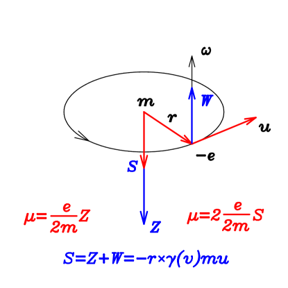
Figure 4: This model represents the circular motion, at the speed of light, of the center of charge of the electron in the center of mass frame. The center of mass is always a different point that the center of charge. The radius of this motion is $R_{0}=\hbar/2mc$, in this frame. The angular velocity is $\omega_{0}=2mc^{2}/\hbar$. This frequency, decreases when the center of mass moves. The local clock slows down when moving. The spin has two contributions: one ${\bi Z}$ from the orbital motion of the CC around the CM (Zitterbewegung) and another ${\bi W}$ in the opposite direction, related to the rotation with angular velocity $\boldsymbol{\omega}$ of a comoving Cartesian frame attached to the CC. The magnetic moment is related to the motion of the CC, and therefore to the zitterbewegung contribution to the spin, ${\bi Z}$, with a normal relation ${\boldsymbol{\mu}}=e{\bi Z}/2m$. It is when we express the magnetic moment in terms of the total spin ${\bi S}$, when we obtain the concept of gyromagnetic ratio $g=2$ [14].

The position ${\bi r}$ of the CC, satisfies a system of fourth-order differential equations [13], that can be separated into a system of second-order differential equations for the CC and CM positions, where the CM position ${\bi q}$, is defined in terms of the motion of the CC, ${\bi r}$, by

$${\bi q}={\bi r}+\left(\frac{c^{2}-{\bi v}\cdot{\bi u}}{(d^{2}{\bi r}/dt^{2})^{2}}\right)\frac{d^{2}{\bi r}}{dt^{2}},$$ (5)

where ${\bi v}={d{\bi q}}/{dt}$, and ${\bi u}={d{\bi r}}/{dt}$ and $v<c$ and $u=c$. The energy $H$, and the linear momentum ${\bi p}$, are written, as in the case of the point particle model, in terms of the center of mass velocity ${\bi v}$, as:

$$H=\gamma(v)mc^{2},\quad{\bi p}=\gamma(v)m{\bi v}.$$ (6)

The relativistic differential equations in the presence of an external electromagnetic field ${\bi E}(t,{\bi r})$ and ${\bi B}(t,{\bi r})$, defined at the CC position ${\bi r}$, and in any arbitrary inertial reference frame are [13]:

$$\frac{d^{2}{\bi q}}{dt^{2}} = \frac{e}{m\gamma(v)}\left[{\bi E}+{\bi u}\times{\bi B}-\frac{1}{c^{2}}{\bi v}\left(\left[{\bi E}+{\bi u}\times{\bi B}\right]\cdot{\bi v}\right)\right],$$ (7)

$$\frac{d^{2}{\bi r}}{dt^{2}} = \frac{c^{2}-{\bi v}\cdot{\bi u}}{({\bi q}-{\bi r})^{2}}\left({\bi q}-{\bi r}\right),$$ (8)

where $\gamma(v)=(1-{\bi v}^{2}/c^{2})^{-1/2}$, and the constraint $|{\bi u}|=c$. Equation (7) corresponds to

$$\frac{d{\bi p}}{dt}=e\left({\bi E}+{\bi u}\times{\bi B}\right),$$

where ${\bi u}$ is the velocity of the CC, which appears in the magnetic force and ${\bi p}$ is defined in (6). Equation (8) is equation (5) when writing on the left hand side the acceleration of the CC. Taking the second order derivative of ${\bi q}$ in (5) and replacing it by (7) we recover [13] the fourth-order system of differential equations for the CC position ${\bi r}$, which is where the external fields ${\bi E}(t,{\bi r})$ and ${\bi B}(t,{\bi r})$, are defined.

Since this model has two characteristic points, the formalism defines the angular momentum (spin) of the particle with respect to both points ${\bi r}$ and ${\bi q}$. It is found that the spin with respect to the CC, ${\bi r}$, is:

$${\bi S}=-\gamma(v)m({\bi r}-{\bi q})\times{\bi u},$$ (9)

while the spin with respect to the CM, ${\bi q}$, is defined by:

$${\bi S}_{CM}={\bi S}+{(\bi r}-{\bi q})\times{\bi p}=-\gamma(v)m({\bi r}-{\bi q})\times({\bi u}-{\bi v}).$$ (10)

The spins (9) and (10) are finally expressed in terms of the instantaneous separation between both centers and of the velocities of both points, while it is only the velocity of the CM ${\bi v}$, which appears in the definition of $H$ and ${\bi p}$, (6).

For the center of mass observer ${\bi q}={\bi v}=0$, and both spins take the same value in this frame. According to the figure 4, if $R_{0}=|{\bi r}-{\bi q}|$ is the separation between the CC and CM, then the constant value of the spin $S=\hbar/2$,

$$\frac{\hbar}{2}=mcR_{0},\quad\Longrightarrow\quad R_{0}=\frac{\hbar}{2mc}=1.93\cdot 10^{-13}\,{\rm m},$$

and this separation is half Compton’s wavelength, as was mentioned before.

The total angular momentum ${\bi J}$ of the electron with respect to the origin of any arbitrary inertial frame, can be written in two ways as:

$${\bi J}={\bi S}+{\bi r}\times{\bi p}={\bi S}_{CM}+{\bi q}\times{\bi p}.$$

Both spins satisfy different dynamical equations. If the particle is free, ${\bi v}$ is constant and $d{\bi J}/dt=0$, and $d{\bi p}/dt=0$, leads to

$$\frac{d{\bi S}}{dt}={\bi p}\times{\bi u},\quad\frac{d{\bi S}_{CM}}{dt}=0.$$

The CM spin ${\bi S}_{CM}$, is conserved while the spin with respect to the CC, ${\bi S}$, satisfies the same dynamical equation as Dirac’s spin operator in the quantum case. Its time derivative is always orthogonal to the direction of the linear momentum. We must remark that in the quantum Dirac’s analysis, the only variable that defines the position of the electron ${\bi r}$, is contained in Dirac’s spinor $\psi(t,{\bi r})$, and it is also the point where the external electromagnetic field $A_{\mu}(t,{\bi r})$ is defined, and it is moving at the speed $c$. Clearly, the spin with respect to the CC, ${\bi S}$, represents the classical equivalent of Dirac’s spin operator.

The spin ${\bi S}$ has two parts: one ${\bi Z}$ associated to this relative internal motion and to the dependence of the Lagrangian on the acceleration and another ${\bi W}$ in the opposite direction related to the dependence of the Lagrangian on the angular velocity of a local Cartesian frame attached to the motion of the center of charge. This frame is not depicted in the figure. The magnetic moment of the electron is produced by the motion of the charge (zitterbewegung) and is related to the orbital part ${\bi Z}$ of the angular momentum by ${\boldsymbol{\mu}}=e{\bi Z}/2m$. When the magnetic moment is expressed in terms of the total spin ${\bi S}$, which is half the orbital part ${\bi Z}$, is when we obtain the concept of gyromagnetic ratio $g=2$, [14].

The energy can also be written in the form:

$$H={\bi p}\cdot{\bi u}+\frac{1}{c^{2}}{\bi S}\cdot\left(\frac{d{\bi u}}{dt}\times{\bi u}\right),$$ (11)

which contains two terms: the first term, proportional to the linear momentum, represents the translational energy, while the second, proportional to the spin and to the motion of the CC (zitterbewegung), represents the rotational energy which never vanishes. If we introduce in (11) the expressions of ${\bi p}$ and ${\bi S}$, given in (6) and (9), respectively, we get $H=\gamma(v)mc^{2}$. It is this linear expression in terms of $H$ and ${\bi p}$, which will give rise to Dirac’s Hamiltonian when quantizing the model [11]. In the quantum description $H=i\hbar\partial/\partial t$ and ${\bi p}=-i\hbar\nabla$ and (11) is transformed into Dirac equation.

The angular velocity corresponds to the rotation of a comoving Cartesian frame linked to the point ${\bi r}$. But this frame is completely arbitrary. Once the CC is moving, its dynamics defines the acceleration ${\bi a}$, orthogonal to the velocity ${\bi u}$, and therefore these two orthogonal vectors with the vector ${\bi u}\times{\bi a}$ define an orthogonal comoving frame (the Frenet-Serret frame), so that the angular velocity of this frame can be expressed as

$$\boldsymbol{\omega}=\frac{1}{c^{2}}{\bi u}\times{\frac{d{\bi u}}{dt}}.$$

The evolution of the angular velocity is determined by the motion of the CC. In this way, the above rotational part of the Hamiltonian (11) is just $-{\bi S}\cdot{\boldsymbol{\omega}}>0$, because the spin has the direction opposite to the angular velocity of this frame. The classical equivalent to Dirac’s Hamiltonian (11) can also be written as $H={\bi p}\cdot{\bi u}-{\bi S}\cdot{\boldsymbol{\omega}}$, where the translation and rotation energies are more evident.

In the Lagrangian description we started with a mechanical system of 6 degrees of freedom. Three represent the position of a point ${\bi r}$, and another three angles $\boldsymbol{\alpha}$, that describe the orientation of a comoving frame. The dynamics has established a constraint such that the degrees of freedom $\boldsymbol{\alpha}$ are finally related to the motion of ${\bi r}$, that satisfies a system of fourth-order differential equations. This point and their derivatives, completely determine the definition of any other observable. The electron description has been reduced to the evolution of a single point, the center of charge.

6.1 Planck and de Broglie hypothesis

The manifold spanned by the variables $(t,{\bi r},{\bi u},\boldsymbol{\alpha})$, where $t\in\mathbb{R}$, ${\bi r}\in\mathbb{R}^{3}$, ${\bi u}\in\mathbb{R}^{3}$ with $u<c$, and $\boldsymbol{\alpha}\in SO(3)$, is the Poincaré group manifold. The submanifold with the constraint $u=c$, is a homogeneous space of the Poincaré group. According to the Atomic Principle it can represent the boundary variables manifold of the Lagrangian description of a classical elementary particle. In this manifold two different kinds of elementary particles can be described [12]. One possibility is that the velocity ${\bi u}$ is a constant vector and the point moves along a straight line with constant velocity $c$, and the comoving frame rotates with angular velocity $\boldsymbol{\omega}$ in the same direction, pointing forward or backwards. This is the classical description of a photon. The free Lagrangian of a photon is

$$L_{0}=\epsilon\frac{S}{c}{\bi u}\cdot\boldsymbol{\omega},$$

where $\epsilon=\pm 1$, represents the helicity. The spin ${\bi S}=\partial L_{0}/\partial\boldsymbol{\omega}=\epsilon S{\bi u}/c$, and is not transversal. The linear momentum ${\bi p}=\partial L_{0}/\partial{\bi u}=\epsilon S\boldsymbol{\omega}/c$ and also has the same direction than the velocity ${\bi u}$. All four vectors, ${\bi p}$, ${\bi u}$, ${\bi S}$ and $\boldsymbol{\omega}$ are collinear vectors. The energy of the photon has two expressions $H={\bi p}\cdot{\bi u}=pc={\bi S}\cdot{\boldsymbol{\omega}}=S\omega$. If $S=\hbar$ then $H=\hbar\omega=h\nu$, which is Planck’s hypothesis concerning the quanta of the electromagnetic field. The photon is a boson.

The other possibility is that ${\bi u}\cdot d{\bi u}/dt=0$, and gives rise to the Dirac particle described in the figure 4. It is a system of six degrees of freedom, ${\bi r}$ and $\boldsymbol{\alpha}$. If we analyze this particle for the center of mass observer, and we choose the reference frame in such a way that the angular velocity (and the spin) is along $OZ$ axis, it is reduced to a system of three degrees of freedom: the $x$ and $y$ coordinates of the point on the $XOY$ plane and the phase $\alpha$ of the comoving Cartesian frame attached to the point. But the dynamics produces the constraint that the comoving frame can be the Frenet-Serret frame and the phase $\alpha$ is exactly the phase of the rotational circular motion of the point ${\bi r}$. But if the point describes a circle of radius $R_{0}$, given the coordinate $x$, the coordinate $y$ is determined so that we are left with a system of just one degree of freedom for the center of mass observer. This degree of freedom $x$, represents a one-dimensional harmonic oscillator of pulsation $\omega_{0}$ in this frame. According to the Atomic Principle it has no excited states and therefore it is a one-dimensional harmonic oscillator in its ground state. The energy of this particle (${\bi p}=0$) is $H=-{\bi S}\cdot{\boldsymbol{\omega}}=S\omega_{0}=\hbar\omega_{0}/2$, which gives $S=\hbar/2$. This object is a fermion. Because the center of mass is at rest then $mc^{2}=\hbar\omega_{0}/2$, and the internal frequency $\nu_{0}=2mc^{2}/h$, is not the postulated de Broglie’s frequency but rather the frequency predicted by Dirac, twice de Broglie’s frequency. In this formalism the Dirac particle has been reduced in the center of mass frame to a one-dimensional harmonic oscilator with no excited states.

6.2 Boundary Conditions

To integrate the system of differential equations (7) and (8), we have to establish the appropriate boundary conditions for the positions and velocities of both points, the CC and the CM. These 12 boundary values for the variables ${\bi r}(0)$, ${\bi u}(0)$, ${\bi q}(0)$ and ${\bi v}(0)$, are going to be expressed in terms of 10 parameters. These 10 parameters are those parameters that define the relationship between the center of mass observer and any arbitrary inertial observer or laboratory observer.

If $t^{*}$ and ${\bi r}^{*}$ are the time and position of the CC for the center of mass observer $O^{*}$, and $t$ and ${\bi r}$ are the time and position of the CC for any arbitrary inertial observer, they are related by the Poincaré transformation:

$$x^{\mu}=\Lambda^{\mu}_{\nu}x^{*\nu}+a^{\mu},\quad x^{\mu}\equiv(ct,{\bi r}),\quad x^{*\mu}\equiv(ct^{*},{\bi r}^{*}),\quad a^{\mu}\equiv(cb,{\bi d}),$$

and $\Lambda=L({\bi v})R(\psi,\theta,\phi)$ is a general Lorentz transformation, as a composition of a rotation $R$, followed by a boost or pure Lorentz transformation $L$.

We are going to describe now the rotation $R(\psi,\theta,\phi)$, the boost or pure Lorentz transformation $L({\bi v})$ with arbitrary velocity ${\bi v}$, the space translation $T({\bi d})$ of displacement ${\bi d}$, and finally the time translation $T(b)$, of value $b$.

Let us first analyze the rotation. Let us assume we have the Dirac particle in the center of mass reference frame, as depicted in figure 5, with the spin along $OZ$ axis.

Figure 5: Dirac particle in the center of mass reference frame, with the spin along the OZ axis. The initial position of the CC on the $XOY$ plane is determined by the phase $\psi$.

If we initially have the CC at the position $(R_{0},0,0)$ on the $OX$ axis, we rotate first an angle $\psi$, around the $OZ$ axis to modify the CC position. Next, we change the orientation of the spin by modifying the zenithal angle $\theta$, and azimuthal angle $\phi$, so that the arbitrary rotation is the composition of the rotations

$$R(\psi,\theta,\phi)=R_{OZ}(\phi)R_{OY}(\theta)R_{OZ}(\psi),$$

$$R_{OZ}(\psi)=\pmatrix{\cos\psi&-\sin\psi&0\cr\sin\psi&\cos\psi&0\cr 0&0&1},$$

$$R_{OY}(\theta)=\pmatrix{\cos\theta&0&\sin\theta\cr 0&1&0\cr-\sin\theta&0&\cos\theta},\quad R_{OZ}(\phi)=\pmatrix{\cos\phi&-\sin\phi&0\cr\sin\phi&\cos\phi&0\cr 0&0&1}.$$

If initially at time $t^{*}_{0}$, the CC is at the point $(R_{0},0,0)$, then the position, velocity and acceleration of the CC, before the rotation, are:

$${\bi r}^{*}(t^{*}_{0})=R_{0}\pmatrix{1\cr 0\cr 0},\quad{\bi u}^{*}(t^{*}_{0})=c\pmatrix{0\cr-1\cr 0},\quad{\bi a}^{*}(t^{*}_{0})=c\omega_{0}\pmatrix{-1\cr 0\cr 0}.$$

These variables, after the rotation, become ${\bi r}^{*}_{0}=R_{OZ}(\phi)R_{OY}(\theta)R_{OZ}(\psi){\bi r}^{*}(t^{*}_{0})$, and the same for ${\bi u}^{*}(t^{*}_{0})$ and ${\bi a}^{*}(t^{*}_{0})$, at the same time $t^{*}_{0}$, and thus:

$${\bi r}^{*}_{0}=R_{0}\pmatrix{\cos\theta\cos\phi\cos\psi-\sin\phi\sin\psi\cr\cos\theta\sin\phi\cos\psi+\cos\phi\sin\psi\cr-\sin\theta\cos\psi},$$ (12)

$${\bi u}^{*}_{0}=c\pmatrix{\cos\theta\cos\phi\sin\psi+\sin\phi\cos\psi\cr\cos\theta\sin\phi\sin\psi-\cos\phi\cos\psi\cr-\sin\theta\sin\psi},$$ (13)

$${\bi a}^{*}_{0}=-c\omega_{0}\pmatrix{\cos\theta\cos\phi\cos\psi-\sin\phi\sin\psi\cr\cos\theta\sin\phi\cos\psi+\cos\phi\sin\psi\cr-\sin\theta\cos\psi}.$$ (14)

A Lorentz transformation of velocity ${\bi v}$, is given by the $4\times 4$ matrix

$$L({\bi v})=\pmatrix{\gamma&\gamma{v_{x}/c}&\gamma{v_{y}/c}&\gamma{v_{z}/c}\cr\gamma{v_{x}/c}&1+{\displaystyle v_{x}^{2}\over\displaystyle c^{2}}{\displaystyle\gamma^{2}\over\displaystyle\gamma+1}&{\displaystyle v_{x}v_{y}\over\displaystyle c^{2}}{\displaystyle\gamma^{2}\over\displaystyle\gamma+1}&{\displaystyle v_{x}v_{z}\over\displaystyle c^{2}}{\displaystyle\gamma^{2}\over\displaystyle\gamma+1}\cr\gamma{v_{y}/c}&{\displaystyle v_{y}v_{x}\over\displaystyle c^{2}}{\displaystyle\gamma^{2}\over\displaystyle\gamma+1}&1+{\displaystyle v_{y}^{2}\over\displaystyle\displaystyle c^{2}}{\displaystyle\gamma^{2}\over\displaystyle\gamma+1}&{\displaystyle v_{y}v_{z}\over\displaystyle c^{2}}{\displaystyle\gamma^{2}\over\displaystyle\gamma+1}\cr\gamma{v_{z}/c}&{\displaystyle v_{z}v_{x}\over\displaystyle c^{2}}{\displaystyle\gamma^{2}\over\displaystyle\gamma+1}&{\displaystyle v_{z}v_{y}\over\displaystyle c^{2}}{\displaystyle\gamma^{2}\over\displaystyle\gamma+1}&1+{\displaystyle v_{z}^{2}\over\displaystyle c^{2}}{\displaystyle\gamma^{2}\over\displaystyle\gamma+1}\cr},$$ (15)

where $\gamma\equiv(1-(v_{x}/c)^{2}-(v_{y}/c)^{2}-(v_{z}/c)^{2})^{-1/2}$. Finally the two translations $T({\bi d})$ and $T(b)$. The corresponding time $t_{0}$ and position ${\bi r}_{0}$ of the CC of the same event, for any arbitrary inertial observer are:

$$t_{0}=\gamma\left(t^{*}_{0}+\frac{{\bi v}\cdot{\bi r}^{*}_{0}}{c^{2}}\right)+b,\quad{\bi r}_{0}={\bi r}^{*}_{0}+\gamma{\bi v}t^{*}_{0}+\frac{\gamma^{2}}{1+\gamma}\frac{({\bi v}\cdot{\bi r}^{*}_{0}){\bi v}}{c^{2}}+{\bi d},$$

where $b$ is the time translation, ${\bi d}$ is the space translation and ${\bi v}$ is the velocity of the center of mass observer $O^{*}$ as measured by the observer $O$. It represents, therefore, the velocity of the center of mass of the particle for the arbitrary laboratory observer $O$.

If the initial instant to integrate the equations in the reference frame of the observer $O$, is the time $t_{0}=0$, this corresponds to $\gamma t^{*}_{0}=-\gamma{\bi v}\cdot{\bi r}^{*}_{0}/{c^{2}}-b$, for the center of mass observer, and therefore the initial position of the CC for the laboratory observer at the initial instant $t_{0}=0$, is:

$${\bi r}_{0}={\bi r}^{*}_{0}-\frac{\gamma}{1+\gamma}\frac{({\bi v}\cdot{\bi r}^{*}_{0}){\bi v}}{c^{2}}-b{\bi v}+{\bi d}.$$ (16)

For the remaining observables,

$${\bi u}_{0}=\frac{{\bi u}^{*}_{0}+\gamma{\bi v}+\frac{\gamma^{2}}{(1+\gamma)c^{2}}{({\bi v}\cdot{\bi u}^{*}_{0}){\bi v}}}{\gamma(1+{\bi v}\cdot{\bi u}^{*}_{0}/c^{2})},$$ (17)

$${\bi a}_{0}=\frac{(1+{\bi v}\cdot{\bi u}^{*}_{0}/c^{2}){\bi a}^{*}_{0}-({\bi v}\cdot{\bi a}^{*}_{0}/c^{2}){\bi u}^{*}_{0}-\frac{\gamma}{(1+\gamma)c^{2}}({\bi v}\cdot{\bi a}^{*}_{0}){\bi v}}{\gamma^{2}(1+{\bi v}\cdot{\bi u}^{*}_{0}/c^{2})^{3}},$$ (18)

where ${\bi r}^{*}_{0}$, ${\bi u}^{*}_{0}$ and ${\bi a}^{*}_{0}$ are given above in (12), (13) and (14), respectively.

With these values we have the initial boundary conditions for the variables ${\bi r}_{0}$, ${\bi u}_{0}$, ${\bi v}_{0}={\bi v}$. What we have left is ${\bi q}_{0}$, the initial position of the CM in this reference frame.

The definition of the center of mass position in any reference frame is given in (5), then the initial value of the CM ${\bi q}_{0}$, in the laboratory frame is:

$${\bi q}_{0}={\bi r}_{0}+\frac{c^{2}-{\bi v}\cdot{\bi u}_{0}}{{{\bi a}_{0}}^{2}}\,{\bi a}_{0},$$

in terms of the position, velocity and acceleration of the CC in this reference frame and of the velocity of the CM, all this variables defined at the initial time $t_{0}$.

As a summary, the boundary conditions at $t_{0}=0$, in the laboratory frame, are:

$${\bi r}_{0}={\bi r}^{*}_{0}-\frac{\gamma}{1+\gamma}\frac{({\bi v}\cdot{\bi r}^{*}_{0}){\bi v}}{c^{2}}-b{\bi v}+{\bi d},$$ (19)

$${\bi u}_{0}=\frac{{\bi u}^{*}_{0}+\gamma{\bi v}+\frac{\gamma^{2}}{(1+\gamma)c^{2}}{({\bi v}\cdot{\bi u}^{*}_{0}){\bi v}}}{\gamma(1+{\bi v}\cdot{\bi u}^{*}_{0}/c^{2})},$$ (20)

$${\bi q}_{0}={\bi r}_{0}+\frac{c^{2}-{\bi v}\cdot{\bi u}_{0}}{{{\bi a}_{0}}^{2}}\,{\bi a}_{0},$$ (21)

$${\bi v}_{0}={\bi v},$$ (22)

with ${\bi a}_{0}$ given in (18), and the magnitudes ${\bi r}^{*}_{0}$, ${\bi u}^{*}_{0}$ and ${\bi a}^{*}_{0}$, are those which appear in (12-14).

Figure 6: Initial position of the CM when the velocity ${\bi v}$ and the spin direction form an angle $\theta$. It is perpendicular to the vectors ${\bi v}$ and ${\bi u}^{*}_{0}\times{\bi r}^{*}_{0}$, of distance to the center $O-CM=v\sin\alpha$, in natural units, and is independent of the initial position of the CC.

Since ${\bi a}^{*}_{0}=-(\omega_{0}c/R_{0}){\bi r}^{*}_{0}=-\omega_{0}^{2}{\bi r}^{*}_{0}$, taking the squared of (18) we get

$${{\bi a}_{0}}^{2}=\frac{\omega_{0}^{2}c^{2}}{\gamma^{4}(1+{\bi v}\cdot{\bi u}^{*}_{0}/c^{2})^{4}},$$

From (17) the term

$$c^{2}-{\bi v}\cdot{\bi u}_{0}=\frac{c^{2}}{\gamma^{2}(1+{\bi v}\cdot{\bi u}^{*}_{0}/c^{2})},$$

$$\frac{c^{2}-{\bi v}\cdot{\bi u}_{0}}{{\bi a}_{0}^{2}}{\bi a}_{0}=\frac{\gamma^{2}}{\omega_{0}^{2}}(1+{\bi v}\cdot{\bi u}^{*}_{0}/c^{2})^{3}{\bi a}_{0},$$

and if we substitute for ${\bi a}_{0}$ the expression (18), where ${\bi a}^{*}_{0}=-\omega_{0}^{2}{\bi r}^{*}_{0}$, the initial position of the CM, ${\bi q}_{0}$, instead of (21), is

$${\bi q}_{0}=\frac{1}{c^{2}}{\bi v}\times({\bi u}^{*}_{0}\times{\bi r}^{*}_{0})-b{\bi v}+{\bi d}.$$ (23)

In general, the initial position of the CM for the laboratory observer, given in (23), is contained in the zitterbewegung plane (with ${\bi d}=0=b$), is independent of the initial position of the CC, ${\bi r}^{*}_{0}$, and is depicted in the figure 6. The distance to the center is $(v/c)\sin\alpha$. If ${\bi v}$ is perpendicular to the ziterbewegung plane, ${\bi v}\cdot{\bi r}^{*}_{0}={\bi v}\cdot{\bi u}^{*}_{0}=0$, and the CM is at the center of the circle and becomes equidistant of the trajectory of the CC. If ${\bi v}$, has a different orientation, the separation between both centers CC and CM, $|{\bi r}-{\bi q}|$, is not a constant of the motion.

6.3 Natural units

We have a natural unit of velocity $c$, and a natural unit of length, the radius $R_{0}$ of the zitterbewegung motion for the center of mass observer. If we define the dimensionless variables $\widetilde{\bi r}={\bi r}/R_{0}$, $\widetilde{t}=\omega_{0}t$, with $\omega_{0}=c/R_{0}$, then

$${\bi u}=\frac{d{\bi r}}{dt}=R_{0}\frac{d\widetilde{\bi r}}{d\widetilde{t}}\omega_{0}=c\frac{d\widetilde{\bi r}}{d\widetilde{t}},$$

$$\frac{d{\bi u}}{dt}=c\frac{d^{2}\widetilde{\bi r}}{d\widetilde{t}^{2}}\omega_{0}=\frac{c^{2}}{R_{0}}\frac{d^{2}\widetilde{\bi r}}{d\widetilde{t}^{2}}.$$

and therefore the differential equation (8) in natural units is

$$\frac{d^{2}\widetilde{\bi r}}{d\widetilde{t}^{2}}=\frac{1-\widetilde{\bi v}\cdot\widetilde{\bi u}}{(\widetilde{\bi q}-\widetilde{\bi r})^{2}}(\widetilde{\bi q}-\widetilde{\bi r}),$$

where now $0\leq\widetilde{v}<1$ and $\widetilde{u}=1$. For the equation (7) in natural units, we arrive to,

$$\frac{c^{2}}{R_{0}}\frac{d^{2}\widetilde{\bi q}}{d\widetilde{t}^{2}}=\frac{e}{m\gamma}\left[{\bi E}+\widetilde{\bi u}\times{\bi B}c-\widetilde{\bi v}\,\left({\bi E}+\widetilde{\bi u}\times{\bi B}c\right)\cdot\widetilde{\bi v}\right],$$

and by using that $R_{0}=\hbar/2mc$, we get:

$$\frac{d^{2}\widetilde{\bi q}}{d\widetilde{t}^{2}}=\frac{A}{\gamma(\widetilde{v})}\left[{\bi E}+\widetilde{\bi u}\times{\bi B}c-\widetilde{\bi v}\,\left({\bi E}+\widetilde{\bi u}\times{\bi B}c\right)\cdot\widetilde{\bi v}\right],$$ (24)

where

$$A=\frac{e\hbar}{2m^{2}c^{3}}=3.778\cdot 10^{-19}\;{\rm C\,kg^{-1}m^{-1}s^{2}}.$$

The external fields ${\bi E}$ and ${\bi B}$, are expressed in the international system of units and are defined, at every instant in the laboratory frame, at the position of the CC, ${\bi r}$, and the parameter $A$ is for the electron.

The 12 boundary conditions in the natural system of units are:

$$\widetilde{\bi r}_{0}=\widetilde{\bi r}^{*}_{0}-\frac{\gamma}{1+\gamma}(\widetilde{\bi v}\cdot\widetilde{\bi r}^{*}_{0})\widetilde{\bi v}-\widetilde{b}\widetilde{\bi v}+\widetilde{\bi d},\quad\widetilde{\bi u}_{0}=\frac{\widetilde{\bi u}^{*}_{0}+\gamma\widetilde{\bi v}+\frac{\gamma^{2}}{(1+\gamma)}{(\widetilde{\bi v}\cdot\widetilde{\bi u}^{*}_{0})\widetilde{\bi v}}}{\gamma(1+\widetilde{\bi v}\cdot\widetilde{\bi u}^{*}_{0})},$$ (25)

$$\widetilde{\bi q}_{0}=\widetilde{\bi v}\times(\widetilde{\bi u}^{*}_{0}\times\widetilde{\bi r}^{*}_{0})-\widetilde{b}\widetilde{\bi v}+\widetilde{\bi d},\quad\widetilde{\bi v}_{0}=\widetilde{\bi v},$$ (26)

where

$$\widetilde{\bi r}^{*}_{0}={\bi r}^{*}_{0}/R_{0},\quad\widetilde{\bi u}^{*}_{0}={\bi u}^{*}_{0}/c,$$

${\bi r}^{*}_{0}$ and ${\bi u}^{*}_{0}$ are given, respectively in (12) and (13).

$$\widetilde{b}=\omega_{0}b,\quad\widetilde{\bi d}={\bi d}/R_{0},$$

The values of $b$ and ${\bi d}$ are in the international system of units and $\gamma\equiv\gamma(\widetilde{v})$.

6.4 Dirac particle in a uniform magnetic field

We are going to describe the motion of the Dirac particle in a uniform magnetic field. To depict in the same picture the cyclotronic motion of the center of mass, that has a radius of order of $10^{-6}$m in a magnetic field of 5 Teslas, and the zitterbewegung motion of the center of charge of smaller radius $R_{0}\simeq 10^{-13}$m, we have to consider a higher velocity electron and a very large magnetic field, to appreciate in this picture, both motions.

In a uniform magnetic field along $OZ$ axis ${\bi B}=B{\bi e}_{z}$, the dynamical equation (24) in natural units becomes

$$\frac{dv_{x}}{dt}=\frac{KB}{\gamma(v)}\left[u_{y}-v_{x}(v_{x}u_{y}-v_{y}u_{x})\right],$$

$$\frac{dv_{y}}{dt}=\frac{KB}{\gamma(v)}\left[-u_{x}-v_{y}(v_{x}u_{y}-v_{y}u_{x})\right],$$

$$\frac{dv_{z}}{dt}=\frac{KB}{\gamma(v)}\left[-v_{z}(v_{x}u_{y}-v_{y}u_{x})\right],\quad K=\frac{e\hbar}{2m^{2}c^{2}}=1.13273\cdot 10^{-10},$$

where all the tildes have been removed and the magnetic field is given in Teslas.

For the initial conditions in natural units

$$\theta=30^{\circ},\phi=90^{\circ},\quad v_{y}(0)=0.1,\quad d_{x}=5,\quad b=0,$$

and a magnetic field of $B=2\cdot 10^{8}$, we get the cyclotronic motion of the CM of radius $R_{c}\simeq 5$ and zitterbewegung motion of the CC of internal radius 1, of the figure 7.

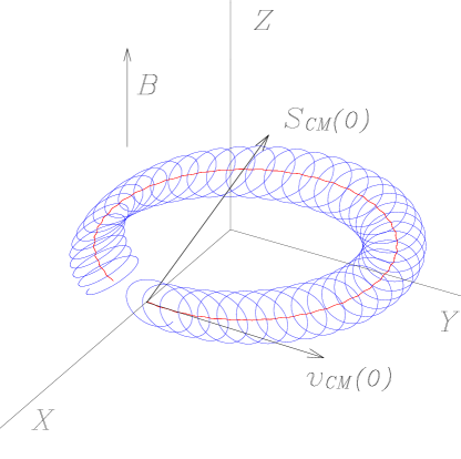
Figure 7: Cyclotronic motion of the CM (red) and zitterbewegung motion of the CC (blue), with $v/c=0.1$, spin orientation $\theta=30^{\circ}$, $\phi=90^{\circ}$ and $B=2\cdot 10^{8}$.

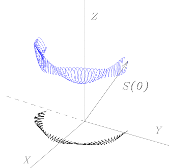
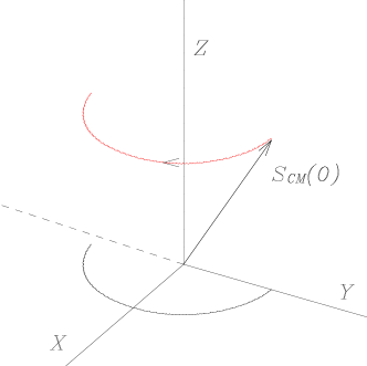
Figure 8: Evolution of the end point of the CC spin ${\bi S}$ (blue) and its projection onto the XOY plane(black) and the evolution of the CM spin ${\bi S}_{CM}$ (red) and its projection onto the XOY plane(black), corresponding to the same time of the evolution of figure 7. Both spins precess backwards with the angular velocity $-\omega_{c}/2$.

We also depict on figure 8, the evolution of both spins, the CC spin ${\bi S}$ and the CM spin ${\bi S}_{CM}$ during the same time of the evolution of the figure 7. The CC spin moves in the orthogonal direction to the linear momentum, because it satisfies Dirac’s dynamical equation $d{\bi S}/dt={\bi p}\times{\bi u}$. Here the time derivative of the spin is always orthogonal to the direction of the linear momentum. We see that the CM spin behaves like the average of the CC spin. Both spins precess backwards with the angular velocity $\omega_{s}$, half the cyclotronic angular velocity $\omega_{s}=-\omega_{c}/2$. This is in contradiction with the assumption of the experimental works [4]-[8], where it is assumed that the spin precession angular velocity is $\omega_{s}=g\omega_{c}/2$.

In the figure 9 we depict the same cyclotronic motion, with the same spin orientation, $\theta=30^{\circ}$, $\phi=90^{\circ}$, but now the magnetic field is smaller than in the previous integration $B=9\cdot 10^{6}$. The initial velocity $v/c=0.1$ is the same, but produces a bigger cyclotronic radius $R_{c}\approx 100$, in dimensionless units. This scale corresponds to a cyclotronic motion of radius $R_{c}\approx 10^{-11}$m. The trajectories of the CC and CM with a separation of order $R_{0}\approx 10^{-13}$m, appear too close together to be able to distinguish them separately. Nevertheless the spin evolution is exactly the same as before. It precess backwards with the angular velocity $\omega_{s}=-\omega_{c}/2$.

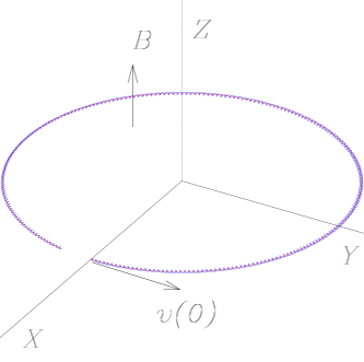
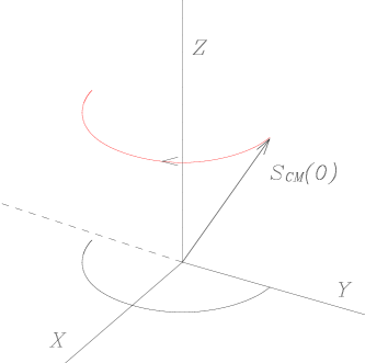
Figure 9: Cyclotronic motion of radius $R_{c}\approx 100$ of the CC and CM, and the evolution of the CM spin ${\bi S}_{CM}$ (red) with the same orientation as in the figure 8, and its projection onto the XOY plane(black), during the same time as the cyclotronic motion on the left. The initial velocity is $v=0.1$ and the magnetic field $B=9\cdot 10^{6}$. As before, the CM spin ${\bi S}_{CM}$ precess backwards with the angular velocity $-\omega_{c}/2$.

With a magnetic field of 5 Teslas, the inicial velocity like in the other examples $v/c=0.1$, the cyclotronic radius is $R_{c}\approx 10^{8}$ in natural units, but the motion of the spin is the same as in the above figure 9, where the ${\bi S}_{CM}$, precess backwards with the angular velocity $-\omega_{c}/2$.

6.5 Definition of magnetic moment for the Dirac particle

According to Jackson [15], the magnetic moment of a current density ${\bi j}(t,{\bi r})$ with respect to a point, which we take as the origin of our reference frame, is defined as the vector:

$$\boldsymbol{\mu}=\frac{1}{2}\int{\bi r}\times{\bi j}(t,{\bi r})dV.$$ (27)

where $dV$ is the volume element around the point ${\bi r}$. In the case of a flat closed circuit of area $A$ and intensity $I$, the above definition leads for the absolute value of $\mu$, to $\mu=IA$.

For a point particle of charge $e$, located at the point ${\bi r}$, and moving at the velocity ${\bi v}$, the instantaneous magnetic moment with respect to the origin of the reference frame, compatible with the above definition (27), is:

$$\boldsymbol{\mu}=\frac{1}{2}e{\bi r}\times{\bi v},$$ (28)

since $e{\bi v}$, plays the role of ${\bi j}(t,{\bi r})dV$. If the point particle has mass $m$, the relativistic angular momentum with respect to the origin of the reference frame is

$${\bi J}={\bi r}\times{\bi p}=m\gamma(v){\bi r}\times{\bi v},\quad\Longrightarrow\quad\boldsymbol{\mu}=\frac{e}{2m\gamma(v)}{\bi J},$$ (29)

and we find a relationship between the instantaneous magnetic moment and the angular momentum with respect to the same point, for the spinless point particle.

In the model of the Dirac particle of charge $e$, depicted in the figure 4, moving in circles of radius $R_{0}$ at the speed $c$, the period of this motion is $T_{0}={2\pi R_{0}}/{c}$, and this motion is equivalent to a current of intensity $I=e/T_{0}$. The area enclosed is $A=\pi R_{0}^{2}$, and the absolute value of the magnetic moment, according to the definition (27), is:

$$\mu_{B}=IA=\frac{e\hbar}{2m},$$

which is called Bohr’s magneton. When expressed this $\mu_{B}$ in terms of the spin with respect to the center $S=\hbar/2$, it takes the form:

$$\mu_{B}=2\frac{e}{2m}\frac{\hbar}{2}=g\frac{e}{2m}S,\quad\Rightarrow\quad g=2,$$

and the quantity $g=2$, which is absent in the definition of the magnetic moment for the spinless electron (29), is called the gyromagnetic ratio. This expression for the magnetic moment and its relation with the angular momentum for the relativistic Dirac particle is different than in the case of the relativistic spinless point particle (29).

Therefore, for the Dirac particle, the relationship between its magnetic moment with respect to the CM and the spin with respect to the CM, should include the factor $g=2$, and, instead of (29), will be

$$\boldsymbol{\mu}_{CM}=\frac{e}{m\gamma(v)}{\bi S}_{CM}.$$ (30)

In this work we are going to consider that $g/2$ is not an intrinsic property of the electron, but rather it is a magnitude related to the ratio of the experimental measurement of the absolute value of the magnetic moment and the absolute value of the theoretical prediction. We take, for the Dirac particle, as the exact relationship between the instantaneous magnetic moment and the spin with respect to the center of mass, the above definition (30).

Using the expression of ${\bi S}_{CM}$ in (10) the appropriate definition of the instantaneous magnetic moment with respect to the center of mass of the electron, in terms of the classical variables which describe its motion, will be:

$${\boldsymbol{\mu}}_{CM}=-e({\bi r}-{\bi q})\times({\bi u}-{\bi v}),$$ (31)

which lacks the factor $1/2$ of the corresponding definition for the spinless point particle (28). In the case of the Dirac particle at rest, the instantaneous magnetic moment and its average value are the same, and the absolute value is,

$$\mu=eR_{0}c=\frac{e\hbar}{2m}=\mu_{B}.$$

6.6 Definition of electric dipole moment for the Dirac particle

The definition of the instantaneous electric dipole moment for a system of point particles of charges $q_{i}$, located at the respective points ${\bi r}_{i}$, with respect to the origin of the reference frame, is

$${\bi d}=\sum_{i}q_{i}{\bi r}_{i}.$$

In the case of the Dirac particle, the electric dipole moment with respect to the CM is:

$${\bi d}_{CM}=e({\bi r}-{\bi q}).$$ (32)

For the Dirac particle at rest, this dipole is not a constant of the motion. Its average value during a turn of the charge is 0, but the absolute value is the constant $d_{CM}=eR_{0}$. Therefore, the measurement of the electron dipole moment is equivalent to the measurement of the average separation between the CM and CC, and the existence of this dipole is not related to any asymmetry of the possible charge distribution. In chapter 6 of [3] we have shown that the above classical definition of electric dipole moment (32) leads, when quantizing this model, to Dirac’s electric dipole moment operator. We arrive to this result by making use of Hestenes geometric algebra [16]. We also show that the absolute value of this dipole gives rise to Darwin’s term of Dirac’s Hamiltonian.

7 Dirac particle in a Penning trap

In the Penning trap of section 2, the electromagnetic field is

$${\bi E}=\frac{V_{0}R_{0}}{2d^{2}}(r_{x},r_{y},-2r_{z}),\quad{\bi B}=(0,0,B),$$

with $V_{0}$ in Volts, $B$ in Teslas and the magnetron dimension $d$ in meters. The fields are defined at the CC position ${\bi r}$, of the electron, in natural units.

We are going to integrate the above dynamical equations with the data of the experiment performed by Gabrielse and Dehlmet [4], where the fields and parameters take the values:

$$V_{0}=10.22\,{\rm V},\quad B=5.872\,{\rm T},\quad d=0.00335\,{\rm m}.$$

If we express the variables in the fields in terms of dimensionless variables, the dynamical equations of the Dirac particle in the Penning trap are:

$$\frac{dq_{x}}{dt}=v_{x},\quad\frac{dq_{y}}{dt}=v_{y},\quad\frac{dq_{z}}{dt}=v_{z},$$

$$\frac{dv_{x}}{dt}=\frac{1}{\gamma(v)}\left[C(r_{x}-v_{x}(v_{x}r_{x}+v_{y}r_{y}-2v_{z}r_{z}))+K(u_{y}+v_{x}u_{y}-v_{y}u_{x})\right],$$

$$\frac{dv_{y}}{dt}=\frac{1}{\gamma(v)}\left[C(r_{y}-v_{y}(v_{x}r_{x}+v_{y}r_{y}-2v_{z}r_{z}))+K(-u_{x}+v_{x}u_{y}-v_{y}u_{x})\right],$$

$$\frac{dv_{z}}{dt}=\frac{1}{\gamma(v)}\left[-C(2r_{z}+v_{z}(v_{x}r_{x}+v_{y}r_{y}-2v_{z}r_{z}))+K(v_{x}u_{y}-v_{y}u_{x})\right],$$

$$\frac{dr_{x}}{dt}=u_{x},\quad\frac{dr_{y}}{dt}=u_{y},\quad\frac{dr_{z}}{dt}=u_{z},$$

$$\frac{du_{x}}{dt}=\frac{1-v_{x}u_{x}-v_{y}u_{y}-v_{z}u_{z}}{(q_{x}-r_{x})^{2}+(q_{y}-r_{y})^{2}+(q_{z}-r_{z})^{2}}(q_{x}-r_{x}),$$

$$\frac{du_{y}}{dt}=\frac{1-v_{x}u_{x}-v_{y}u_{y}-v_{z}u_{z}}{(q_{x}-r_{x})^{2}+(q_{y}-r_{y})^{2}+(q_{z}-r_{z})^{2}}(q_{y}-r_{y}),$$

$$\frac{du_{z}}{dt}=\frac{1-v_{x}u_{x}-v_{y}u_{y}-v_{z}u_{z}}{(q_{x}-r_{x})^{2}+(q_{y}-r_{y})^{2}+(q_{z}-r_{z})^{2}}(q_{z}-r_{z}),$$

where the dimensionless coefficients are:

$$C=\frac{e\hbar V_{0}}{4d^{2}m^{2}c^{3}}=-1.72043\cdot 10^{-13},$$

$$K=\frac{e\hbar B}{2m^{2}c^{2}}=-6.65139\cdot 10^{-10}.$$

and

$$\gamma(v)=(1-v_{x}^{2}-v_{y}^{2}-v_{z}^{2})^{-1/2}.$$

All tildes above the position and velocity variables have been withdrawn and they are considered from now on dimensionless variables.

The predicted features of the classical description, where the internal motion of the CC is a very high frequency motion $\omega_{0}\simeq 10^{21}$ s^-1, imply that when we try to perform some measurement, for instance, the instantaneous value of any magnitude, like positions and velocities of points, they are impossible to determine. Every measurement takes some time, so that what we understand by the classical measurement of any observable is the time average value of sufficient local measurements, all of them performed with the same method and under the same or equivalent conditions.

In this integration what we are going to measure first is the absolute value of the electric dipole moment (32), which, when compared with its value at rest $d_{0}=eR_{0}$, is just $|\widetilde{R}|=|{\bi r}-{\bi q}|$, in dimensionless units. This separation vector between the CC and CM is not a constant vector. The time average value is 1 for the free particle, and will be greater than 1 when moving. To determine its value, we shall calculate the time average value of this expression during a complete number of turns of the CC. With the electron at rest, the time to complete a turn is $T_{0}=2\pi R_{0}/c=2\pi$, in natural units. If the CM of the Dirac particle is moving at the speed $v$, then the time during a complete turn is $T=\gamma(v)T_{0}$. Therefore, the time average value of this separation for a Dirac particle $\widetilde{R}(v)$, after $n$ turns of the CC, is defined as

$$\widetilde{R}(v)=\frac{1}{2\pi n\gamma(v)}\int_{0}^{2\pi n\gamma(v)}\,|{\bi r}-{\bi q}|\,dt.$$

The other measurement is the absolute value of the magnetic moment with respect to the center of mass. Compared with the Bohr magneton

$$\frac{\mu_{CM}}{\mu_{B}}=|({\bi r}-{\bi q})\times({\bi u}-{\bi v})|,$$

in dimensionless units. This measurement will be the equivalent to the value $g/2$ of the mentioned experiments, but for the free particle is 1 and it is going to be $\leq 1$ for interacting particles, and not greater than 1 as is suggested by the aforementioned magnetic moment experiments.

We are going to compute these magnitudes for $n=100$ turns. For the velocity of the center of mass of the electron we take the three values $v_{y}=0.1,\;0.01,\;0.001$, which correspond to a cyclotronic radius of value $2.9\cdot 10^{-5},\;2.9\cdot 10^{-6},\;2.9\cdot 10^{-7}\;$m, respectively. For every velocity we take seven spin orientations $\alpha$, with respect to the velocity vector, of values $\alpha=90^{\circ},\;80^{\circ},\;60^{\circ},\;45^{\circ},\;30^{\circ},\;10^{\circ},\;0^{\circ}\;$. We reproduce the following three tables corresponding to the different velocities.

The table for $v=0.1$,
$\alpha$ $v_{y}$ $v\sin\alpha$ $|{\bi r}-{\bi q}|/R_{0}$ $\mu_{CM}/\mu_{B}$ $90^{\circ}$ 0.1 0.1 1.0049942672 0.989993718551 $80^{\circ}$ 0.1 0.09848077 1.0048428413 0.990146042526 $60^{\circ}$ 0.1 0.08660254 1.0037436229 0.991244492210 $45^{\circ}$ 0.1 0.07071067 1.0024936295 0.992492125834 $30^{\circ}$ 0.1 0.05 1.0012436541 0.993738193060 $10^{\circ}$ 0.1 0.0173648 1.0001444234 0.994832676462 $0^{\circ}$ 0.1 0 0.9999936553 0.994982699773

The table for $v=0.01$,
$\alpha$ $v_{y}$ $v\sin\alpha$ $|{\bi r}-{\bi q}|/R_{0}$ $\mu_{CM}/\mu_{B}$ $90^{\circ}$ 0.01 0.01 1.0000499974 0.999899998972 $80^{\circ}$ 0.01 0.00984807 1.0000484905 0.999901506625 $60^{\circ}$ 0.01 0.00866025 1.0000374888 0.999912498864 $45^{\circ}$ 0.01 0.00707106 1.0000249983 0.999924998628 $30^{\circ}$ 0.01 0.005 1.0000124986 0.999937498238 $10^{\circ}$ 0.01 0.00173648 1.0000015065 0.999948490080 $0^{\circ}$ 0.01 0 0.9999999989 0.999949997690

Finally the table for $v=0.001$,
$\alpha$ $v_{y}$ $v\sin\alpha$ $|{\bi r}-{\bi q}|/R_{0}$ $\mu_{CM}/\mu_{B}$ $90^{\circ}$ 0.001 0.001 1.0000004990 0.999998999929 $80^{\circ}$ 0.001 0.00098480 1.0000004769 0.999999014972 $60^{\circ}$ 0.001 0.00086602 1.0000003677 0.999999124895 $45^{\circ}$ 0.001 0.00070710 1.0000002430 0.999999249895 $30^{\circ}$ 0.001 0.0005 1.0000001245 0.999999374895 $10^{\circ}$ 0.001 0.00017364 1.0000000148 0.999999484817 $0^{\circ}$ 0.001 0 0.9999999999 0.999999499894

The expected measurement of the electric dipole moment is the product of the constant $eR_{0}=3.09344\cdot 10^{-32}\;$Asm times the obtained value of $|{\bi r}-{\bi q}|$. This time average value is not a constant of the motion and depends on the value $v_{\alpha}=v\sin\alpha$, which is related to the initial separation between the CM and CC, as we mention before (see figure 6). The smaller this magnitude $v_{\alpha}$, smaller is the time average value of the absolute value of the dipole ${\bi d}_{e}$.

For the time average of the magnetic moment with respect to the CM, we also see that the absolute value is not a constant, it also depends on the value $v_{\alpha}$, and when the velocity is smaller it approaches the value 1 of the free particle. The magnetic moment decreases when the CM velocity increases. The absolute value of the magnetic moment with respect to the center of mass is always a little bit smaller than the predicted theoretical value by Dirac.

From the experimental point of view, the determination of this separation $|{\bi r}-{\bi q}|$, can also be obtained by the measurement of the internal angular velocity of the CC, since $R_{0}=c/\omega_{0}$. An experiment of the type of Gouanére et al. [17] will ellucidate whether the internal frequency of the electron is the frequency postulated by De Broglie $\omega_{0}/2$, or Dirac’s predicted frequency $\omega_{0}$, which is the frequency of this model as described in 6.1. It has been suggested to enlarge the energy range of the above experiment [18], to measure this internal frequency.

The integrations of this work have been performed numerically by means of the computer package Dynamics Solver [19]. It uses a Dorman-Price 8(5,3) integration code. All codes have adaptive step size control and we check that smaller tolerances do not change the results. The electric dipole moment is computed with 10 decimal digits while the ratio $\mu/\mu_{B}$ with 12. More accuracy can be obtained by taking the time average over a greater number of turns. For instance, with $v=0.01$, when the spin and the velocity form an angle of $60^{\circ}$, the ratio is $\mu/\mu_{B}=0.999912498864$, computed with $n=100$ turns, while for $n=300$ turns gives the value $\mu/\mu_{B}=0.999912496757$, where the difference is at the 9th decimal position.

8 Conclusions

Dirac’s theory predicts the exact factor $g=2$ in the definition of the magnetic moment [1]. In a non-relativistic framework Levy-Leblond’s equation [20] also predicts $g=2$, as well as in the classical model of Dirac particle analyzed here [3]. However, when we try to measure the magnetic moment we have to interact with the electron. The interaction modifies the motion of the CC and CM of the electron and this justifies that the measurement of the magnetic moment could be different than the theoretical prediction for the electron at rest.

The conclusions about the measurements of the magnetic moment and the electric dipole moment of the electron are based on the analysis of the classical electron model with spin that leads to Dirac equation when quantized, described in section 6.

The main characteristic of this model is that the dynamics of the electron is the description of the motion of a single point ${\bi r}$, that is considered the center of charge of the electron. Furthermore, the electron has another characteristic point, the center of mass ${\bi q}$, which is always a different point from the center of charge.

If the electron has two characteristic points then it must be clear with respect to which point the angular momentum, i.e., the spin, is defined. In Dirac’s theory we have that Dirac’s spinor depends only on a point ${\bi r}$, where the external fields are defined, and therefore, it is interpreted as the center of charge of the electron. Dirac’s spin is defined with respect to this point ${\bi r}$. This spin is never conserved. If we consider the angular momentum with respect to the center of mass it is a conserved angular momentum for the free particle and which precess backwards with half the cyclotronic angular velocity in a magnetic field.

The magnetic moment is produced by the movement of the center of charge around the center of mass, also known in the physics literature as the zitterbewegung, which is a motion with curvature and torsion. The electric dipole moment is due to the separation between these two points and not to an asymmetric distribution of the electron charge. It is not along the spin direction but it is oriented on a plane orthogonal to the spin and rotates with the angular velocity $\omega_{0}$. Both momenta are defined with respect to the center of mass.

The internal motion at the speed of light is of a such high frequency that from the classical point of view the measurement of the observables must be interpreted as a time average over a sufficiently long time. We have solved numerically the dynamical equations of the model in a Penning trap of the same characteristics and fields as in one of the experiments. In the classical description we have assumed no thermal interaction and that the fields and smoothness of the cavity are the ones described theoretically. The only available theory of radiation is the theory for spinless electrons where the center of mass and center of charge are the same point. Radiation is produced whenever the electron is accelerated, which in the classical spinning model would correspond to the acceleration of the center of mass. The theory of radiation for spinning particles is not ready yet. Therefore we have consider no radiation in the above numerical analysis.

Measuring the electric dipole moment of the electron is measuring the average separation between the center of mass and center of charge of the electron. In no case does this have anything to do with the spin precession but it depends on the velocity of the center of mass $v$ and the orientation $\alpha$ of this velocity with respect to the center of mass spin. This average value of the electric dipole moment is a little bigger than the predicted theoretical value in Dirac’s formalism and in our model. It is not an intrinsic property and its measurement depends on $v\sin\alpha$.

The conjecture that the magnetic moment of the electron has the value $\mu=(g/2)\mu_{B}$, where $g$ is considered an intrinsic property, is an erroneous conjecture since the measurement of the time average value of the magnetic moment does not produce a single value, but a value that is somewhat a little bit smaller than the theoretical prediction. It also depends on the value $v\sin\alpha$. It is clear that if we accept that the spin precession angular velocity is $\omega_{s}=g\omega_{c}/2$, the accurate measurement of these two angular velocities leads to a single result for the magnitude $g$. But this is a wrong definition of this magnitude, only related to the spin precession angular velocity and not to the motion of the charge.

The center of mass spin needs two cyclotronic turns to come back to its initial position because $\omega_{s}=-\omega_{c}/2$. This property is probably related to the geometrical description of spinors which need a rotation of $4\pi$ to come back to its initial situation and that is related to the doubly connected structure of the rotation group.

The historical and critical analysis carried out by Consa [21] on the theoretical and experimental measurement of the gyromagnetic ratio, as one of the greatest successes of Quantum Electrodynamics, casts doubt on the validity of both, the experiments and the theoretical analysis based on a theory full of divergences. We believe in the precision and validity of the experimental results but they are based on a wrong theoretical interpretation of the magnitudes they are trying to measure.

Regarding the efforts to accomodate the computed theoretical results to the experimental data of a magnitude like $g$, that is not an intrinsic property of the electron, it makes us think that this is an inconsistent theoretical approach.

If the theoretical analysis of this paper helps to design new experimental setups for measuring electron properties, the time spent on it will be considered well spent.

References

References

- [1] P.A.M Dirac, (1928) The Quantum Theory of the Electron, Proc. Roy. Soc. London A 117, 610.
- [2] P.A.M Dirac, (1930) The Principles of Quantum Mechanics, Oxford University Press.
-
[3]
M. Rivas (2001),
Kinematical Theory of Spinning Particles, Fundamental Theories of Physics Series, Vol 116, Dordrecht, Holland.
Updated versions of this formalism can be obtained at the web site of the Zitter-Institute, under the publications of the author, https://www.zitter-institute.org - [4] G. Gabrielse and H.G. Dehmelt, (1981) Faster, simpler schemes to distinguish n=0,1 in Geonium, Bull. Am. Phys. Soc. 26, 59.
- [5] R.S. Van Dyck, Jr., P.B. Schwinger and H.G. Dehmelt,(1986), Electron magnetic moment from geonium spectra: Early experiments and background concepts, Phys. Rev. D, 34 722-736.
- [6] R.S. Van Dyck, Jr., P.B. Schwinger and H.G. Dehmelt,(1987), Phys. Rev. Lett. 59 26.
- [7] X. Fan, T.G. Myers, B.A.D. Sukra and G. Gabrielse (2023), Measurement of the electron magnetic moment, Phys. Rev. Lett. 130(7) 071801; arXiv:2209.13084v2.
- [8] D. Hanneke, S. Fogwell and G. Gabrielse (2008), New measurement of the Electron Magnetic Moment and the Fine Structure Constant, Phys. Rev. Lett. 100, 120801.
- [9] ACME Collaboration (2013), Order of magnitude Smaller Limit on the Electric Dipole Moment of the Electron, arXiv:1310.7534.
- [10] M. Rivas (2008), The atomic hypothesis: Physical consequences, J. Phys. A, 41, 304022.
- [11] M. Rivas (1994), Quantization of generalized spinning particles. New derivation of Dirac’s equation, J. Math. Phys. 35, 3380.
- [12] M. Rivas (1989), Classical Relativistic Spinning Particles, J. Math. Phys, 30, 318.
- [13] M. Rivas (2003), The dynamical equation of the spinning electron, J. Phys. A, 36, 4703.
- [14] M. Rivas, J.M. Aguirregabiria and A. Hernández (1999), A pure kinematical explanation of the gyromagnetic ratio of leptons and charged bosons, Phys. Lett. 257, 21.
- [15] J.D. Jackson (1998), Classical Electrodynamics, John Wiley.
- [16] D. Hestenes (1966), Space-Time Algebra, Gordon and Breach, NY.
- [17] M. Gouanére, M. Spiegel, N. Cue, M.J. Gaillard, R. Genre, R. Kirsch, J.C. Poizat, J. Remillieux, P. Catillon and L. Roussel (2005), Experimental observation compatible with the particle internal clock, Annales Fondation Louis de Broglie 30, 109.
- [18] M. Rivas (2008), Measuring the internal clock of the electron, arXiv: 0809.3635.
- [19] J.M. Aguirregabiria (2006) Dynamics Solver, computer program for solving different kinds of dynamical systems, which is available from his author through the web site of the Theoretical Physics Dept. of The University of the Basque Country, Bilbao, Spain.
- [20] J.M Levy-Leblond (1967), Non-relativistic particles and wave equations, Comm. Math. Phys. 6, 28.6
- [21] O. Consa (2021), Something is wrong on the state of QED, arXiv:2110.02078.