Hidden Variables unseen by Random Forests

Abstract

Random Forests are widely claimed to capture interactions well. However, some simple examples suggest that they perform poorly in the presence of certain pure interactions that the conventional CART criterion struggles to capture during tree construction. We argue that simple alternative partitioning schemes used in the tree growing procedure can enhance identification of these interactions. In a simulation study we compare these variants to conventional Random Forests and Extremely Randomized trees. Our results validate that the modifications considered enhance the model’s fitting ability in scenarios where pure interactions play a crucial role.

Keywords— random forests;regression tree;cart;pure interaction;functional anova

1 Introduction

Throughout the rise of machine learning over the last decades, decision tree ensembles have captured significant attention. Notably, Breiman’s Random Forests [4] gained widespread popularity among practitioners and has been applied within various fields, e.g. finance, genetics, medical image analysis, among many others [13, 11, 23, 9, 10]. In this paper, we present a simulation study revealing limitations of Random Forests when the target function exhibits certain pure interactions, and we show that adaptions of the algorithm such as Interaction Forests [17] or Random Split Random Forests [3] considerably improve in these scenarios.
Consider a nonparametric regression model

$$Y_{i}=m(X_{i})+\varepsilon_{i},$$

$i=1,\dots,n,$ with i.i.d. data, (unknown) regression function $m:[0,1]^{d}\to\mathbb{R}$ which is measurable and $\varepsilon_{i}$ is zero mean and independent of $X_{i}$. A regression tree is constructed by partitioning the support of $X_{i}$ (feature space) via a greedy top-down procedure known as CART [5]. First, the whole feature space (root cell) is split into two daughter cells by placing a rectangular cut such that the data is approximated well by a function that is constant on each daughter cell. This step is then repeated for each daughter cell and so on, until some stopping criterion is reached. The procedure is called greedy since one optimises the next split given a previous partition instead of optimising the entire partition. We refer to Figure 1 for an illustration.

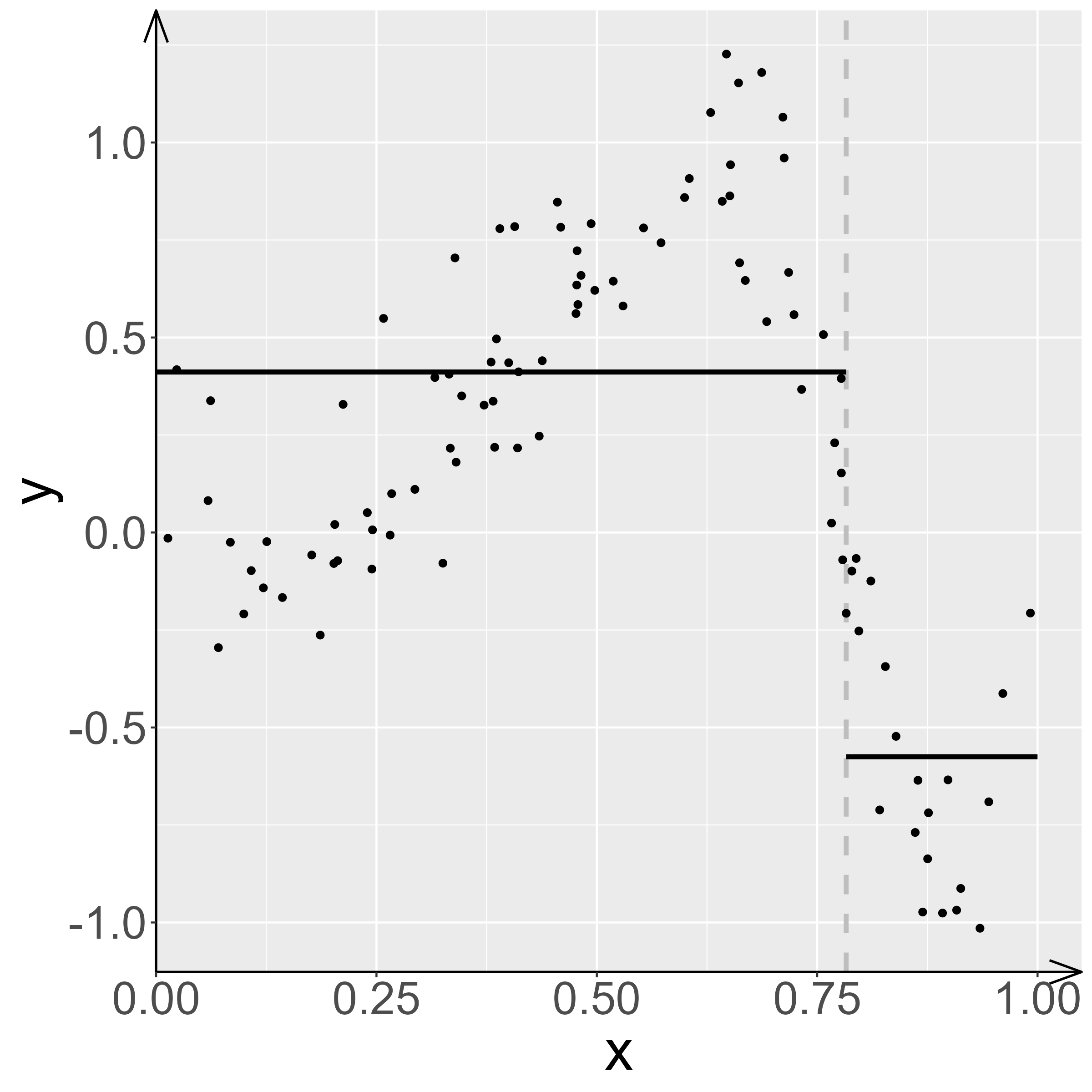
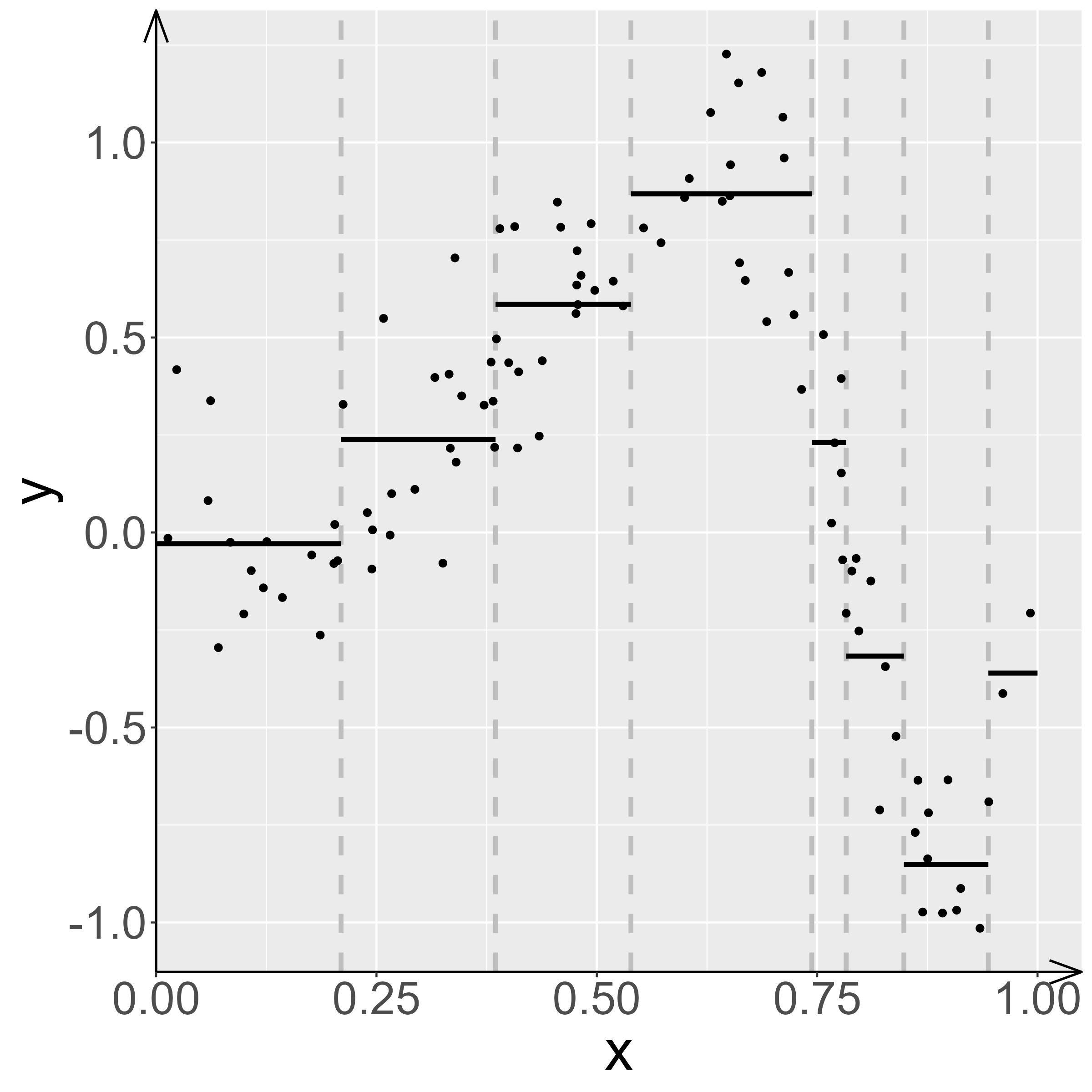
Figure 1: Illustration of the regression tree algorithm for $d=1$. On the left hand side, a single CART split is placed on the $x$-axis (grey dotted line). On the right hand side, the $x$-axis has been split iteratively, resulting in a piece-wise constant estimator (black solid line) of the unknown regression function.

In many situations estimators constructed this way adapt well to high dimensional functions including complex interaction terms. However, difficulties arise in the presence of certain pure interactions. We call interactions between multiple covariates pure if there are no marginal effects present containing exactly one of these covariates. Thus, they are hard to detect when using a step by step procedure using CART, see e.g. [28]. For a formal definition, see Section 2.
In this paper, we consider estimation based on regression tree type methods when pure interaction terms are present. We argue that simple regression trees and Random Forests (even with small mtry parameter value; see Section 2.2.1 for a definition of the mtry parameter) are not able to properly approximate pure interactions. In a large simulation study, we show that different modifications of the tree growing procedure leads to algorithms outperforming Random Forests in these cases.
More precisely, we focus on the Interaction Forests algorithm [17], Random Split Random Forests [3] and Extremely Randomized Trees [12] which have recently been proven to be consistent for regression functions lying in algorithm and data specific function classes [3]. Noteworthy, for Random Split Random Forests (RSRF), the function class where the algorithm is consistent includes regression functions with pure interactions.
While the algorithms have in common that they stick to some of the main principles of Random Forests such as aggregation of individual estimators, the tree growing procedures differ: The modifications include additional randomness when choosing splits, allowing partitions into more than two cells in a single iteration step, and a combination of both.
The difference between trees in the Interaction Forests algorithm [17] and usual CART is that the partition into two cells in a single iteration step is allowed to be constructed through certain cuts along two directions (cf. Figure 4). The authors have shown in a large real data study that Interaction Forests improve upon Random Forests and related methods, in terms of predictive performance.
The RSRF algorithm is based on the following idea: For a predefined $D\in\mathbb{N}$ (depth), split a current cell at random, then split all of its daughter cells at random, and repeat doing so until we have $2^{D-1}$ cells. The $D$th split uses the CART criterion. Thus, we have partitioned the current cell into $2^{D}$ cells. This process is repeated for all resulting cells and so forth. The algorithm is tailored to find interaction terms of orders up to $D$.
We emphasize that the classical mtry parameter of Random Forest does not seem to help with pure interactions. The mtry parameter, for every split, restricts possible split coordinates to randomly chosen subsets of size mtry of the feature coordinates $\{1,\dots,d\}$. If mtry is small enough (for example $\texttt{mtry}=1$), one can guarantee that splits occur in any coordinate. We note that this may help as can be observed in Figure 7 in the appendix. However, as Figure 2 reveals, this does not solve the problem in general and in the setting considered in Figure 2, $\texttt{mtry}=d$, i.e. no randomization, seems to perform best independent of sample size.

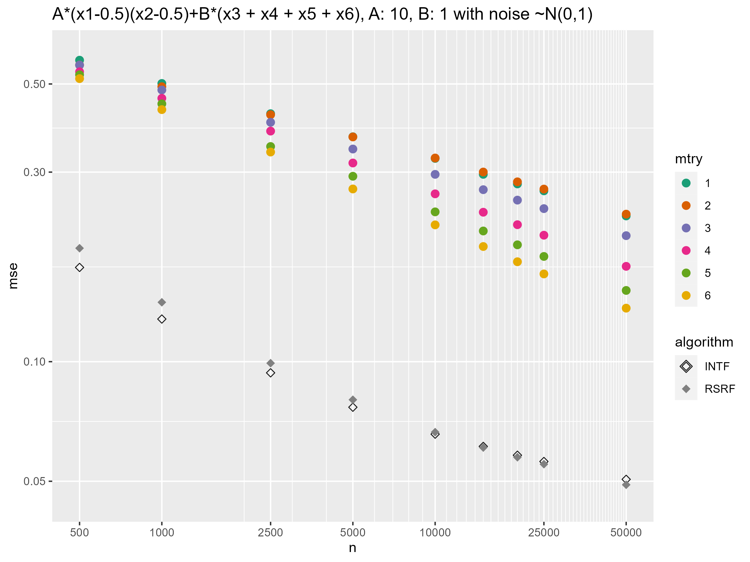
Figure 2: Estimated mean squared error using Random Forests (for different values of mtry), Interaction Forests (INTF) and Random Split Random Forests (RSRF), plotted at $\log$-scales for different sample sizes $n$. The regression model is $Y=10(X_{1}-0.5)(X_{2}-0.5)+X_{3}+X_{4}+X_{5}+X_{6}+\varepsilon$ with regressors $(X_{1},\dots,X_{6})$ uniform on $[0,1]^{6}$ and noise $\varepsilon\sim\mathcal{N}(0,1)$, also see Figure 3. The number of trees was set to $100$ for each of the methods. For each sample size, $100$ simulations were carried out. We note that, when using Random Forests at a sample size of $1$ million, the corresponding error is even larger than the one for INTF / RSRF at a sample size of only $5000$.

Our contribution can be summarized as follows. We show via simulations that Random Forest, independent of hyper-parameter choices, cannot adequately deal with pure interaction terms. In addition, we show in our simulations that the variants discussed above improve upon Random Forests in these situations. An excerpt of our simulation results is given in Table 1.
We emphasize that the focus of this paper is not to promote a specific algorithm, but to show in a simulation study that alternative splitting schemes beyond the simple CART-criterion are necessary for approximating pure interaction terms.

Algorithm	MSE
INTF	$0.151\ (0.028)$
RSRF	$0.195\ (0.032)$
RF	$0.518\ (0.063)$
ET	$0.429\ (0.041)$

Table 1: Excerpt from our simulation study: Reported mean squared error estimates for different simulations in the regression model $Y=10(X_{1}-0.5)(X_{2}-0.5)+X_{3}+X_{4}+X_{5}+X_{6}+\varepsilon$ with $\varepsilon\sim\mathcal{N}(0,1)$ and sample size $n=500$. Standard deviations are provided in brackets. Hyper-parameters for each method are optimally tuned.

In the literature, there exist different algorithms that are both related to Random Forests and designed for models with interactions. Apart from Interaction Forests and RSRF, related algorithms include Bayesian Additive Regression Trees [7], Random Planted Forests [14] and Iterative Random Forests [1]. In [14], it is allowed to keep leafs after a split, resulting in so-called Planted trees. Furthermore, the celebrated Bayesian Additive Regression Trees [7] algorithm fits a sum of parameterized regression trees by updating trees using a bayesian backfitting procedure. In a classification setting [1], interactions are identified by re-weighting the probability vector for choosing an allowed split coordinate in CART (after each tree was built), using a variable importance measure.
Various variants of Random Forests have been designed for specific purposes, e.g. in survival analysis [18], quantile estimation [21], ranking problems [8], or estimation of heterogenous treatment effects [26]. In [2] a general review over Random Forests and its variants is provided, including stylized algorithms used in theoretical analyses. For recent theoretical results on consistency for regression trees that use the CART splitting criterion, we refer to [6, 19, 25, 20, 3].

1.1 Organisation of the paper

The paper is structured as follows. In Section 2, we introduce the notion of pure interactions and formally introduce the CART criterion. Then, we discuss why CART is not an appropriate splitting criterion in case of pure interactions. Section 2.1 describes Interaction Forests and RSRF, while Section 2.2 provides an overview over all algorithms considered in our simulations study. The results of our simulation study are presented and discussed in Section 3.

2 Hidden variables unseen by Random Forests

We introduce the notion of pure interactions and discuss why the CART algorithm has problems dealing with them.

Definition 2.1 (Functional ANOVA decomposition [24, 15]).

We say that the regression function $m$ is decomposed via a functional ANOVA decomposition if

$$m(x)=\sum_{u\subseteq\{1,\dots,d\}}m_{u}(x_{u}),$$

with identification constraint that for every $u\subseteq\{1,\dots,d\}$ and $k\in u$,

$$\int m_{u}\left(x_{u}\right)\int p(x)\mathrm{d}x_{-u}\ \mathrm{d}x_{k}=0,$$

where $p(x)$ is the density of $X$.

We shall discuss the issue by means of the following notion of simple pure interaction between two variables. The discussion can be expanded to more general cases.

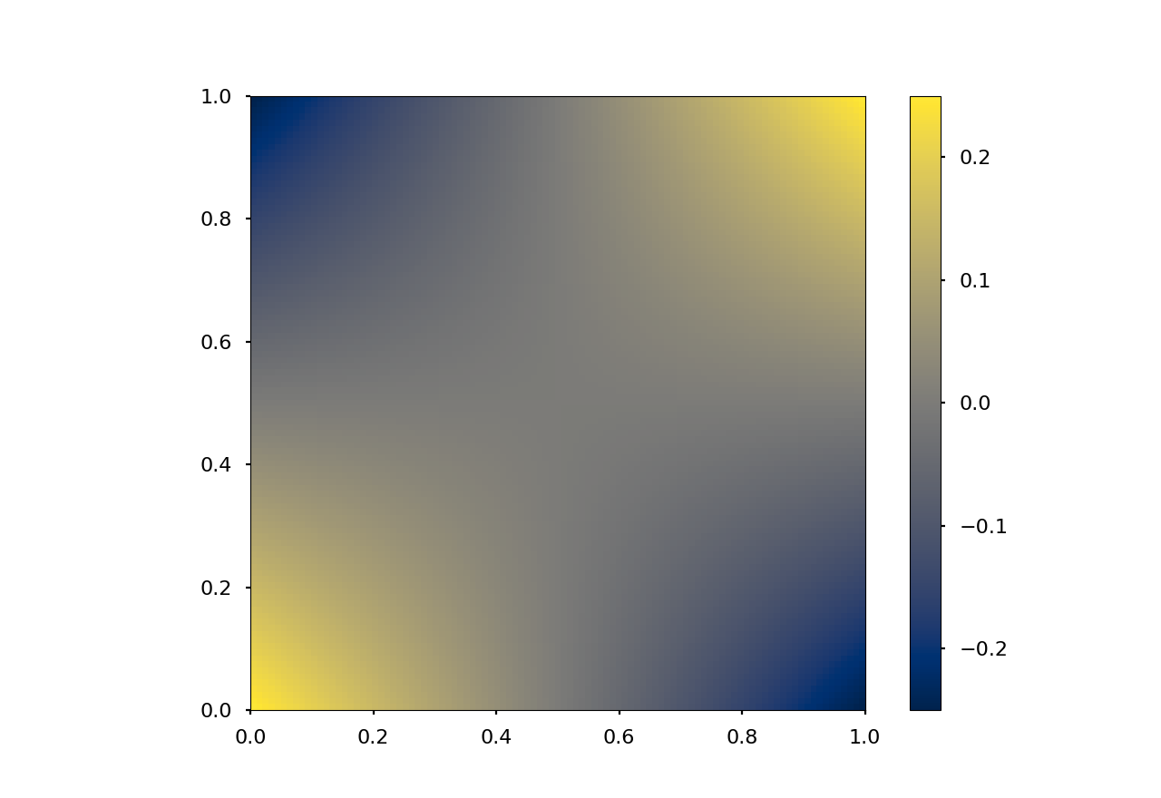
Figure 3: Plot of the function $g:[0,1]^{2}\to\mathbb{R}$, $g(x_{1},x_{2})=(x_{1}-0.5)(x_{2}-0.5)$. Taken from [3].

Definition 2.2 (Simple pure interaction effect).

Let $m_{u}$, $u\subseteq\{1,\dots,d\}$ be the components of the functional ANOVA decomposition of $m$ and $j_{1},j_{2}\in\{1,\dots,d\}$ with $j_{1}\neq j_{2}$. The regression function $m$ has a simple pure interaction effect in $J=\{j_{1},j_{2}\}$ if

• $(X_{j_{1}},X_{j_{2}})$ is independent of $(X_{k}:k\notin\{j_{1},j_{2}\})$,

• $m_{J}\neq 0$,

• $m_{u}=0$ for any $u$ with $j_{1}\in u,j_{2}\notin u$, or with $j_{1}\notin u,j_{2}\in u$.

We need the following property.

Proposition 2.3.

Assume $m$ has a simple pure interaction effect in $\{1,2\}$. Let $I,I_{3},\dots,I_{d}\subseteq[0,1]$ be measurable subsets and suppose

$$t=I\times[0,1]\times I_{3}\times\dots\times I_{d}\text{ or }t=[0,1]\times I\times I_{3}\times\dots\times I_{d}$$

with $\mathbf{P}(X\in t)>0$. Then,

$$\mathbf{E}[m(X)|X\in t]=\mathbf{E}[m(X)|X_{3}\in I_{3},\dots,X_{d}\in I_{d}].$$ (1)

For the proof, see Appendix A in the appendix.
The right hand side of (1) is the expected mean of a node where no split in $\{1,2\}$ has occurred so far. The left hand side considers the conditional mean if that node would next be split in coordinate 1 or 2. We now discuss why algorithms using CART face problems when pure interactions are present. The difficulty lies in the absence of one-dimensional marginal effects guiding to the pure interaction effect, see also [28]. To make this point more concrete for regression trees, let us recall the CART criterion used in regression trees. Suppose $t$ is a rectangular set $t\subseteq[0,1]^{d}$. Write

$$t_{L}=t_{L}(j,s)=\{x\in t:x_{{j}}\leq{s}\},\quad t_{R}=t_{R}(j,s)=\{x\in t:x_{{j}}>{s}\}.$$

for $j\in\{1,\dots,d\}$ and $s\in[0,1]$. One says that $t$ is split at $(j,s)$ into $t_{L}$ and $t_{R}$.

Definition 2.4 (CART criterion, see [5]).

Let $t\subseteq[0,1]^{d}$ and let $J\subseteq\{1,\dots,d\}$. The Sample-CART-split of $t$ is defined as splitting $t$ at coordinate $\hat{j}\in J$ and $\hat{s}\in[0,1]$ into daughter cells where the split point $(\hat{j},\hat{s})$ is chosen from the CART criterion, that is,

$$(\hat{j},\hat{s})\in\ \underset{j\in J,s\in[0,1]}{\arg\min}\bigg{\{} \sum_{i:X_{i}\in t_{L}(j,s)}(Y_{i}-\hat{\mu}_{L})^{2}+\sum_{i:X_{i}\in t_{R}(j,s)}(Y_{i}-\hat{\mu}_{R})^{2}\bigg{\}},$$ (2)

where $\hat{\mu}_{k}=\{\#t_{k}(j,s)\}^{-1}\sum_{i:X_{i}\in t_{k}(j,s)}Y_{i},\ k=L,R$ and $\#t:=\#\{i:X_{i}\in t\}$.

Coming back to the detection of pure interactions, observe that for large samples

$$\begin{split}\eqref{eq:cart-split-criterion1}\times(&\#t)^{-1}\\ \approx\qquad&\mathbf{P}(X\in t_{L}(j,c)|X\in t)\mathbf{E}[(Y-\mathbf{E}[Y|X\in t_{L}(j,c)])^{2}|X\in t_{L}(j,c)]\\ +\ &\mathbf{P}(X\in t_{R}(j,c)|X\in t)\mathbf{E}[(Y-\mathbf{E}[Y|X\in t_{R}(j,c)])^{2}|X\in t_{R}(j,c)],\end{split}$$ (3)

where $(Y,X)$ is distributed as $(Y_{1},X_{1})$.
Now assume that the regression function $m$ has a simple pure interaction effect in features $\{1,2\}$. Then, in view of Proposition 2.3, for any set of the form

$$t=[0,1]^{2}\times I_{3}\times\dots\times I_{d}\subseteq[0,1]^{d},$$

and any $j=1,2$ and $s\in[0,1]$, the right hand side of (3) is equal to $\mathbf{E}[(Y-\mathbf{E}[Y|X\in t])^{2}|X\in t]$. This is the maximal possible value attainable. Hence, in the presence of other features $k=3,\dots,d,$ features $j=1,2$ will probably not be chosen to be split leaving the pure interaction effect undetected. One example is the function $m(x)=A(x_{1}-0.5)(x_{2}-0.5)+B\sum_{k=3}^{d}x_{k}$ for $A,B\neq 0$, with $X_{i}$ uniformly distributed on $[0,1]^{d}$. In this setup, a Sample-CART-split will rarely take on values $\hat{j}=1,2$ if $J\cap\{3,\dots,d\}\neq\emptyset$ and thus the term $A(x_{1}-0.5)(x_{2}-0.5)$ may not be approximated well.

Remark 2.5.

The independence assumption in Definition 2.2 is an extreme scenario. In settings with correlated variables, the variables $1$ and $2$ may not be completely hidden, but our simulations indicate that the CART algorithm still suffers in such scenarios.

2.1 Handling Interactions with Random Forest-type algorithms

In this section we introduce two approaches related to Random Forests, which are designed for settings where (pure) interactions are present. As with Random Forests, both methods are based on aggregation of individual (greedily-built) tree-based estimators. First, we describe the Interaction Forest algorithm from [17]. In a large real data study, the authors demonstrated that Interaction Forests improves upon Random Forests in terms of predictive performance.
Secondly, Random Split Random Forest (RSRF) is introduced. RSRF extends the main principles in Random Forests in order to better handle pure interaction scenarios. We emphasize that studying RSRF is originally motivated from a theoretical perspective. In [3], consistency for a general class of regression tree estimators is established. The RSRF algorithm is then introduced in order to demonstrate that the class of regression functions covered by the theory can differ depending on the specific choice of the partitioning scheme, cf. Section 3 in [3]. In particular, the consistency result for RSRF is valid for a strictly larger function class than the corresponding result for Random Forest. Thus, it appears natural to investigate if a difference in performance in the presence of pure interactions can be observed empirically.

2.1.1 Interaction Forests

Let us describe the individual tree estimators. In each iteration step, cells are split into two daughter cells (that are not necessarily rectangles). Let $t\subseteq\mathbb{R}^{d}$ and two split pairs $(j_{1},c_{1})\in\{1,\dots,d\}\times t^{(j_{1})}$, $(j_{2},c_{2})\in\{1,\dots,d\}\times t^{(j_{2})}$ with $j_{1}\neq j_{2}$ be given, where $t^{(j)}=\{x_{j}:x\in t\}$ is the $j$-th component. Consider the following seven partitions of $t$ into $t_{1}$ and $t_{2}=t\setminus t_{1}$.

In Figure 4 these seven partitions are illustrated.

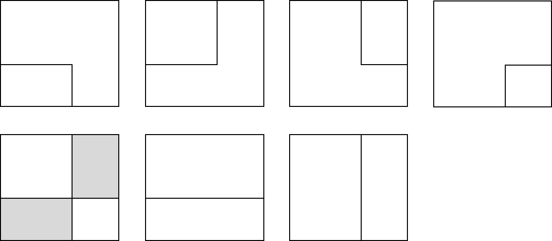
Figure 4: Illustration of possible splits in Interaction Forests. Adapted from [17, Fig. 2] and [3, Fig. 2].

A current cell $t$ is split by first drawing npairs such variable pairs $(j_{1},j_{2})$. For each such pair, seven partitions of the forms above are constructed: First, two split points $c_{1}$ and $c_{2}$ are randomly drawn and used for the two partitions in case (c). Furthermore, another two split points are chosen at random and these are used to construct the five partitions from (a) and (b). We refer to [17, Sec. 4.3] for the details on how valid split points are chosen. In total, one ends up with $7\times\texttt{npairs}$ partitions of $t$ into two sets among which the one with highest decrease in impurity, empirically, is chosen. That is, the quantity $\widehat{\mathbf{S}}$ is used as score, given by

$$\widehat{\mathbf{S}}(t;t_{1},t_{2})=\frac{\#t_{1}}{\#t}\big{[}\hat{\mu}(t_{1})-\hat{\mu}(t)\big{]}^{2}+\frac{\#t_{2}}{\#t}\big{[}\hat{\mu}(t_{2})-\hat{\mu}(t)\big{]}^{2},$$

where $\hat{\mu}(t):=\{\#t\}^{-1}\sum_{i:X_{i}\in t}Y_{i}$.

2.1.2 RSRF: Random Split Random Forests

The algorithm RSRF is another variant of Random Forests. In contrast to Interaction Forests, the cells remain rectangular. The individual predictors are regression trees built using the Random-CART procedure: First, all cells at the current tree depth are split at random, i.e. for each cell, a coordinate is chosen uniformly at random and then, the cell is split at a point chosen uniformly at random along this dimension. Secondly, each of the two resulting cells is split according to the Sample-CART-criterion in (2). We refer to this combination as a “Random-CART-step”. Thus, applying such a Random-CART-step, a cell in the tree is split into four cells. In order to enhance the approach, for a given cell $t$, we shall try several Random-CART-steps as candidates for splitting $t$ into four cells $t_{1,1},t_{1,2},t_{2,1},t_{2,2}$, and then choose the one which is “best” in terms of empirical (2-step) impurity decrease $\widehat{\mathbf{S}}$,

$$\widehat{}\mathbf{S}(t;t_{1,1},t_{1,2},t_{2,1},t_{2,2})=\sum_{\begin{subarray}{c}j=1,2\\ k=1,2\end{subarray}}\frac{\#t_{j,k}}{\#t}\big{[}\hat{\mu}(t_{j,k})-\hat{\mu}(t)\big{]}^{2}.$$ (4)

The number $W$ of candidate Random-CART-steps to try is called the “width parameter”. Furthermore, we may add another candidate split, the “CART-CART-step”, into this comparison: We also split the cell $t$ using the Sample-CART criterion (instead of splitting at random) and then split the daughter cells according to the Sample-CART-criterion, again. We refer to Figures 5 and 6 for illustrations of RSRF. For a detailed description of the algorithm and its implementation, see Appendix B of the appendix.

Figure 5: Illustration of RSRF. The background trees (light gray) illustrate other possible candidate partitions. Adapted from [3].

Figure 6: Illustration of the procedure used by RSRF for splitting a cell $t$ into $t_{11},t_{12},t_{21},t_{22}$. Adapted from [3].

2.2 Overview: Algorithms considered in our simulation study

We compare the following four algorithms in our simulation study.

RF Random Forests [4],

ET Extremely Randomized Trees [12],

INTF Interaction Forests [17],

RSRF Random Split Random Forests [3].

The individual tree estimators used in the four algorithms have in common that the feature space is partitioned iteratively. Another common feature is that, for each cell $t$ which is about to be partitioned in a single iteration step, the impurity decrease $\widehat{\mathbf{S}}$ is used as a score for choosing a partition from a certain set of candidate partitions $P=\{t_{1},\dots,t_{L}\}$ of $t$, where

$$\widehat{\mathbf{S}}(t;P)=\sum_{l=1}^{L}\frac{\#t_{l}}{\#t}[\hat{\mu}(t)-\hat{\mu}(t_{l})]^{2}.$$

For example, the CART splitting criterion in Definition 2.4 is equivalent to maximizing $\widehat{}\mathbf{S}$ when $L=2$ and $P$ ranges over are all rectangular partitions of $t$. Thus, the algorithms are of similar structure, however, they differ through the value of $L$ and the specific form of candidate partitions $P$.

2.2.1 Random Forests

The trees within Random Forests are grown using the CART criterion from Definition 2.4 where, in each iteration step, the set $J\subseteq\{1,\dots,d\}$ is chosen uniformly at random and of size $\#J=$mtry. The parameter mtry is the main hyper-parameter in Random Forests.

2.2.2 Extremely Randomized Trees

Extremely Randomized Trees originate from [12], however, we stick to the implementation from [27]. Here, in each step mtry coordinates are chosen at random, and for each of these, num.random.splits split points are chosen at random within this coordinate. Then, the best split is chosen using $\widehat{\mathbf{S}}$ as criterion. In the extreme case $\texttt{mtry}=\texttt{num.random.splits}=1$, only a single split is randomly chosen in each iteration step, and no criterion is used.

2.3 From trees to a forest

For each of the four algorithms, the final estimator is given by aggregating individual estimators which are of the form

$$\hat{m}_{T}(x)=\sum_{t\in T}\mathbbm{1}_{(x\in T)}\frac{\sum_{i:x_{i}\in t}y_{i}}{\#\{i:x_{i}\in t\}},$$

where $x$ is an element of the feature space and $T$ denotes the leaf nodes obtained from one of the algorithms. In order to aggregate trees to a forest, $B$ trees are grown each based on a bootstrap sample $(x_{i}^{*},y_{i}^{*})$, $i=1,\dots,n$ drawn with replacement from the data. Similarly, subsamples of size smaller than $n$ may be used. In any case, this yields $B$ predictors $\hat{m}_{T^{b}}$ and the final ensemble estimator is obtained by averaging individual tree predictions

$$\hat{m}_{\text{Forest}}(x)=\frac{1}{B}\sum_{b=1}^{B}\hat{m}_{T^{b}}(x),\quad x\in[0,1]^{d}.$$

3 Simulation results

We investigate the performance of the algorithms from Sections 2.1 and 2.2 in a simulation study. We consider $N=100$ Monte-Carlo simulations using the underlying regression model

$$Y^{s}_{i}=m(X_{i}^{s})+\varepsilon_{i}^{s},\quad i=1,\dots,n=500;s=1,\dots,N=100.$$

In total, we investigate five different models (pure-type), (hierarchical), (additive), (pure-2), (pure-3) which are summarized in Table 2. The model (pure-type) is not pure in the sense of Definition 2.2, but it only slightly violates the defining property because of correlation.
For (pure-3), the number of covariates was set to $d=6$. For all other models we chose $d=4,10,30$. The following distributional assumptions were made. For models (pure-2) and (pure-3), we assume that $X_{i}$ is uniformly distributed on $[0,1]^{d}$. For models (pure-type), (hierarchical) and (additive), we follow [22] (see also [14]) and set

$$X_{i,k}^{s}=2.5\pi^{-1}\arctan(\widetilde{X}_{i,k}^{s}),\quad k=1,\dots,d,$$

where $\tilde{X}_{i}^{s}=(\widetilde{X}_{i,1}^{s}\dots,\widetilde{X}_{i,d}^{s})$ follows a $d$-dimensional normal distribution with mean zero and $\mathbf{Cov}(\tilde{X}_{i,k}^{s})=\mathbf{Corr}(\tilde{X}_{i,k}^{s})=0.3$. Note that $X_{i}$ is distributed on $(-1.25,1.25)^{d}$. The $\varepsilon_{i}^{s}$’s are i.i.d. standard normal.

Abbreviation	Regression function
(pure-type)	$m(x)=-2\sin(x_{1}x_{2}\pi)+2\sin(x_{2}x_{3}\pi)$
(hierarchical)	$m(x)=-2\sin(x_{1}\pi)+2\sin(x_{2}\pi)-2\sin(x_{3}\pi)-2\sin(x_{1}x_{2}\pi)+2\sin(x_{2}x_{3}\pi)$
(additive)	$m(x)=-2\sin(x_{1}\pi)+2\sin(x_{2}\pi)-2\sin(x_{3}\pi)$
(pure-2)	$m(x)=5(x_{1}-0.5)(x_{2}-0.5)+5x_{3}$
(pure-3)	$m(x)=10(x_{1}-0.5)(x_{2}-0.5)+x_{3}+x_{4}+x_{5}+x_{6}$

Table 2: Overview of models

Denoting by $\widehat{m}^{s}$ an estimator of $m$ given data $(X_{i}^{s},Y_{i}^{s})_{i=1,\dots,n}$ we measure its accuracy by the mean squared error on an independently generated test set $X^{\text{(test)},s}_{i}$ ($i=1,\dots,500$), i.e.

$$\frac{1}{100}\sum_{s=1}^{100}\left(\frac{1}{500}\sum_{i=1}^{500}\left(\widehat{m}^{s}\big{(}X^{\text{(test)},s}_{i}\big{)}-m\big{(}X^{\text{(test)},s}_{i}\big{)}\right)^{2}\right).$$

Model	Algorithm	$d=4$	$d=10$	$d=30$
	RSRF (CV)	$0.208\ (0.030)$	$0.263\ (0.042)$	$0.389\ (0.077)$
(pure-type)	INTF (CV)	$0.170\ (0.026)$	$0.222\ (0.030)$	$0.325\ (0.056)$
	RF (CV)	$0.311\ (0.068)$	$0.697\ (0.191)$	$1.338\ (0.278)$
	ET (CV)	$0.205\ (0.037)$	$0.395\ (0.158)$	$0.862\ (0.382)$
	mean-Y	$2.137\ (0.150)$	$2.170\ (0.159)$	$2.163\ (0.141)$
	1-NN	$1.281\ (0.115)$	$2.480\ (0.197)$	$3.923\ (0.328)$
	RSRF (CV)	$0.425\ (0.048)$	$0.552\ (0.067)$	$0.682\ (0.072)$
(hierarchical)	INTF (CV)	$0.394\ (0.047)$	$0.515\ (0.058)$	$0.623\ (0.059)$
	RF (CV)	$0.418\ (0.050)$	$0.555\ (0.067)$	$0.677\ (0.071)$
	ET (CV)	$0.361\ (0.044)$	$0.452\ (0.054)$	$0.538\ (0.059)$
	mean-Y	$8.070\ (0.395)$	$8.116\ (0.446)$	$8.062\ (0.455)$
	1-NN	$2.056\ (0.175)$	$5.794\ (0.401)$	$10.505\ (0.803)$
	RSRF (CV)	$0.371\ (0.041)$	$0.472\ (0.056)$	$0.571\ (0.050)$
(additive)	INTF (CV)	$0.343\ (0.041)$	$0.431\ (0.047)$	$0.512\ (0.050)$
	RF (CV)	$0.350\ (0.040)$	$0.460\ (0.051)$	$0.554\ (0.054)$
	ET (CV)	$0.299\ (0.035)$	$0.372\ (0.046)$	$0.430\ (0.048)$
	mean-Y	$5.992\ (0.350)$	$5.933\ (0.310)$	$5.958\ (0.338)$
	1-NN	$1.778\ (0.138)$	$4.252\ (0.289)$	$7.713\ (0.580)$
	RSRF (CV)	$0.155\ (0.027)$	$0.197\ (0.021)$	$0.226\ (0.024)$
(pure-2)	INTF (CV)	$0.127\ (0.024)$	$0.172\ (0.025)$	$0.214\ (0.023)$
	RF (CV)	$0.188\ (0.029)$	$0.235\ (0.023)$	$0.251\ (0.023)$
	ET (CV)	$0.128\ (0.024)$	$0.190\ (0.020)$	$0.209\ (0.021)$
	mean-Y	$2.264\ (0.105)$	$2.269\ (0.111)$	$2.290\ (0.086)$
	1-NN	$1.156\ (0.083)$	$1.872\ (0.136)$	$3.132\ (0.231)$

	Algorithm	$d=6$
	RSRF (CV)	$0.190\ (0.030)$
(pure-3)	INTF (CV)	$0.154\ (0.029)$
	RF (CV)	$0.510\ (0.062)$
	ET (CV)	$0.418\ (0.049)$
	mean-Y	$1.027\ (0.068)$
	1-NN	$1.289\ (0.103)$

Table 3: Reported mean squared error estimates for different simulations. mean-Y uses the mean of the responses as estimator and 1-NN is the $1-$nearest neighbor estimator. Standard deviations are provided in brackets.

We used the $R$-package ranger [27] for Random Forests and Extremely Randomized Trees. For the latter, the option splitrule in ranger is set to “extratrees”. Interaction Forests are implemented in the $R$-package diversityForests [16]. The RSRF algorithm is implemented using $R$ and code is provided in the supplementary material. See also Appendix B in the appendix for details on RSRF.
In order to determine a suitable choice for the hyper-parameters from a set of parameter combinations, we use $10$-fold cross validation (CV). Additionally, we determine “optimal” parameters (opt) chosen in another simulation beforehand. In both cases, $200$ sets of parameter combinations are chosen at random and we refer to Table 4 for the parameter ranges.

Algorithm	Parameter	Value / Range
RSRF	include_cartcart	True, False
	replace	True, False
	width	$1,2,\dots,15\ (d=4,10)$ resp. $1,2,\dots,30\ (d=30)$
	mtry_cart_cart	$1,2,\dots,d$
	mtry_rsrf_step	$1,2,\dots,d$
	min_nodesize	$5,6,\dots,30$
	num_trees	$100$
	mtrymode	not-fixed
RF	num.trees	$500$
	min.node.size	$5,6,\dots 30$
	replace	True, False
	mtry	$1,2,\dots,d$
INTF	num.trees	$500$
	min.node.size	$5,6,\dots 30$
	replace	True, False
	npairs	$1,2,\dots,100\ (d=4)$, resp. $1,2,\dots,150\ (d=6)$,
		resp. $1,2,\dots,250\ (d=10)$ resp. $1,2,\dots,750\ (d=30)$
ET	num.trees	$500$
	min.node.size	$5,6,\dots 30$
	replace	True, False
	num.random.splits	$1,2,\dots,10$
	mtry	$1,2,\dots,d$
	sample.fraction	$1$
	splitrule	extratrees

Table 4: Parameter settings for the different algorithms.

To determine “optimal” parameters we ran $30$ independent simulations on new data $\bar{X}^{s}_{i}$ and test points $\bar{X}^{\text{(test)},s}_{i}$ ($i=1,\dots,500$; $s=1,\dots,30$) and chose the parameter settings for which lowest mean squared error was reported, averaged over $30$ simulations, that is

$$\frac{1}{30}\sum_{s=1}^{30}\left(\frac{1}{500}\sum_{i=1}^{500}\left(\widehat{m}^{s}\big{(}\bar{X}^{\text{(test)},s}_{i}\big{)}-m\big{(}\bar{X}^{\text{(test)},s}_{i}\big{)}\right)^{2}\right).$$

The parameter settings obtained from this search can be found in Section D.2 in the appendix. The results from our simulation can be found in Table 3 (CV) and in Table 7 (opt). In Table 8 the algorithms are ranked from lowest to largest MSE (for the version with optimal parameters). We note that Section D.1 in the appendix contains additional simulations for a slightly different setup of RSRF.

3.1 Discussion of the results

In models where pure interactions are present $\text{(pure-type)},\text{(pure-2)},\text{(pure-3)}$, RSRF and Interaction Forests clearly outperformed Random Forests. Comparing (pure-2) and (pure-3), we see that the gap between the algorithms INTF/RSRF and RF is much larger in (pure-3) where more additive components are present and contribution by the two interacting variables is stronger. The model (additive) is treated equally well by RF and RSRF. The same holds true for the hierarchical interaction model. In every simulation, ET was better than RF. Similarly, INTF was generally better than RSRF. When the parameter npairs is not extremely large, the number of partitions considered in any step for INTF is smaller than the number of partitions for RSRF. This suggests that the Interaction Forests algorithms and the Extremely Randomized Trees algorithm benefit from additional randomization in similar ways.

We note that, in (pure-2), Extremely Randomized Trees was slightly better than RSRF. An inspection of Table 13 reveals that, for each of the mtry coordinates, only a single random splitpoint is drawn. In general, however, we cannot expect to benefit from strong randomization within Extremely Randomized Trees, as the results for (pure-3) suggest.
To sum this up, solely imposing additional randomness to the Sample-CART criterion (2) as is done via mtry in RF, and even more strongly in ET, is not sufficient to obtain good predictive performance in pure interaction models. Indeed, the algorithms INTF/RSRF which use both random splits and different cell partitioning schemes in any step, perform best in the presence of pure interactions.
In Section D.2 in the appendix, tables containing the parameters used for (opt) can be found. Furthermore, for the new RSRF algorithm, we additionally include the top $30$ parameter settings from the parameter search (opt) in the supplementary material and some remarks are included in the appendix, see Section D.3. However, we point out that our aim was not to provide an in-depth analysis on the hyper-parameter choices which would be beyond the scope of the paper.

Supplementary Material

The supplementary material reporting on additional details from the simulation concerning the parameters in RSRF is provided online. The supplement, code for RSRF and for the simulations can be found at https://github.com/rblrblrbl/rsrf-code-paper/. There, we also provide details concerning the software and package versions used in the simulations.

The appendix is structured as follows. We give the proof of Proposition 2.3 in Appendix A. In Appendix B, describes the implementation of RSRF in details, while Appendix C contains a short outline on a possible extension. Lastly, we provide additional material concerning the simulation in Appendix D.

Appendix A Proofs

Proof of Proposition 2.3.

Let $t=A\times[0,1]\times A_{3}\dots\times A_{d}$. Then,

$$\begin{split}\mathbf{E}&[m_{\{1,2\}}(X_{1},X_{2})\mathbbm{1}_{(X\in t)}]\\ &=\int_{t}m_{\{1,2\}}(x_{1},x_{2})p(x_{1},\dots,x_{d})\mathrm{d}x_{1}\cdots\mathrm{d}x_{d}\\ &=\int_{A}\int_{[0,1]}m_{\{12\}}(x_{1},x_{2})p(x_{1},x_{2})\mathrm{d}x_{2}\mathrm{d}x_{1}\int_{A_{3}\times\cdots\times A_{d}}p(x_{3},\dots,x_{d})\mathrm{d}x_{3}\cdots\mathrm{d}x_{d}\\ &=0,\end{split}$$

due to the identification constraint. Thus, $\mathbf{E}[m_{\{1,2\}}(X_{1},X_{2})|X\in t]=0$. More generally, for any $J\supseteq\{1,2\}$,

$$\mathbf{E}[m_{J}(X_{J})|X\in t]=0,$$ (5)

which follows from analogous calculations and the fact that

$$p(x_{1},\dots,x_{d})=p(x_{-J}|x_{J})p(x_{J})=p(x_{-J}|x_{J\setminus\{1,2\}})p(x_{J}),$$

due to independence. Here, we used the notation $x_{J}=(x_{j}:j\in J)$ and $x_{-J}=(x_{j}:j\notin J)$. Now, from (5) and the assumption, we see that

$$\mathbf{E}[m(X)|X\in t]=\sum_{\begin{subarray}{c}u\subseteq\{1,\dots,d\}\\ 1\notin u,2\notin u\end{subarray}}\mathbf{E}[m_{u}(X_{u})|X\in t].$$ (6)

For each $u$ as in the sum,

$$\begin{split}\mathbf{E}[m_{u}(X_{u})|X\in t]&=\frac{\mathbf{E}\big{[}m_{u}(X_{u})\mathbbm{1}_{(X_{1}\in A,X_{2}\in[0,1])}\mathbbm{1}_{(X_{3}\in A_{3})}\cdots\mathbbm{1}_{(X_{d}\in A_{d})}\big{]}}{\mathbf{P}(X_{1}\in A,X_{2}\in[0,1],X_{3}\in A_{3},\dots,X_{d}\in A_{d})}\\ &=\mathbf{E}[m_{u}(X_{u})|X_{3}\in A_{3},\dots,X_{d}\in A_{d}],\end{split}$$ (7)

using independence of $(X_{1},X_{2})$ and $(X_{3},\dots,X_{d})$ in the last step. Note that from letting $A=[0,1]$ in the definition of $t$, by (5), we also have

$$\mathbf{E}[m_{J}(X_{J})|X\in t]=\mathbf{E}[m_{J}(X_{J})|X_{3}\in A_{3},\dots,X_{d}\in A_{d}],$$ (8)

for any $J\supseteq\{1,2\}$. The result then follows from (6) in view of (7) and (8). ∎

Appendix B Detailed description of the RSRF algorithm

We provide details on the implementation of RSRF. An overview of the tree growing algorithm is given below in Remark B.1 and an overview over all the parameters is given in Table 5. In Section B.1 we shall introduce all remaining parts of the algorithm. Recall the definition of $\widehat{\mathbf{S}}$ from equation (4).

Remark B.1 (Overview of the RSRF tree growing procedure).

Let $(x_{i},y_{i})_{i=1,\dots,n}$ be given. Starting with $T_{0}=\{\mathfrak{t}\}$ with $\mathfrak{t}=[0,1]^{d}$, for $m=0,2,4,\dots$ apply the following steps to all current leaf nodes $t\in T_{m}$ which contain at least node_size many data points.

1. Draw $0pt$ many pairs $(j^{w},c^{w})$ by choosing $j^{w}\in\{1,\dots,d\}$ uniformly at random, and by drawing $c^{w}$ from the uniform distribution on the data points

   $$\{x_{i,j^{w}}\ :x_{i}\in t\}\setminus\max\{x_{i,j^{w}}:x_{i}\in t\}.$$

2. For each $w=1,\dots,W$ split $t$ at $(j^{w},c^{w})$ into $t^{w}_{1}$ and $t^{w}_{2}$ and then split $t^{w}_{1}$ and $t^{w}_{2}$ according to the Sample-CART criterion in Definition 2.4. This gives a partition $\{t^{w}_{1,1},t^{w}_{1,2},t^{w}_{2,1},t^{w}_{2,2}\}$, for each $w$. If include_cartcart is set to “true”, additionally consider $w=0$ where $t$ is split using the Sample-CART criterion into $t^{0}_{1},t^{0}_{2}$, and then these cells are again split using Sample-CART.

3. Choose the splits with index $w_{\text{best}}\in\underset{w}{\arg\max}\ \widehat{\mathbf{S}}\left(t;t^{w}_{1,1},t^{w}_{1,2},t^{w}_{2,1},t^{w}_{2,2}\right)$.

4. Add $t_{k,j}^{w_{\text{best}}}$ to $T_{m+2}$ for $k,j\in\{1,2\}$.

The parameter $0pt$ is called width parameter. If include_cartcart is “false”, then there are $0pt$ candidate partitions generated in each iteration step. Recall that we refer to the procedure to generate one of the candidate partitions as a Random-CART-step. In the other case, when include_cartcart is “true”, the number of candidates is $0pt+1$, due to adding the CART-CART-step.

Remark B.2.

If the width $W$ is infinity, then the algorithm can be seen as a two-dimensional extension of the Sample-CART criterion, where optimization takes places over $6$ variables, i.e. when optimizing over the split point for the first split, and the split points for the two daughter cells.

Remark B.3.

We distinguish different approaches for determining allowed split coordinates for the Sample-CART splits used in (b) in the above algorithm. These are called mtrymodes and the details are to be found in Section B.1.1.

B.1 Further details on RSRF

We list the remaining features of the algorithm. An overview over the parameters can be found in Table 5.

node_size	Minimum node size for a cell to be split
$0pt$ (Width)	Number of candidate partitions
$B$	Number of trees
replace	If “true” (“false”), bootstrap samples (subsamples) are used.
include_cartcart	If “true”, then the CART-CART step is added to the candidate splits.
mtrymode	Determines whether possible split coordinates remain fixed over candidate partitions, or not.
	fixed:	not-fixed:
mtry_cart_cart	(not available)	Number of possible coordinates to choose for the CART splits in CART-CART step.
mtry_random	Number of possible coordinates to choose from for the Random split.	(not available)
mtry_random_cart	Number of coordinates to choose from when placing a CART-split in Random-CART step

Table 5: Overview over parameters for RSRF.

Placing the random split point

Whenever we place a random split at a cell $t=\bigtimes_{j=1}^{d}t^{(j)}$, we first choose the dimension $j$ uniformly at random from $\{1,\dots,d\}$. Then, a split point is drawn uniformly at random from the data points $\{x_{i,j}\ :x_{i}\in t\}\setminus\max\{x_{i,j}:x_{i}\in t\}$.

Stopping condition

A current leaf will only be split into new leafs if it contains at least $\texttt{node\_size}\in\mathbb{N}$ number of data points.

From trees to a forest

Similar to Random Forests, we generate an ensemble of trees based on bootstrapping or subsampling. The single tree predictions will then be averaged. Denote by $\hat{m}_{\hat{T}}$ the estimator corresponding to the tree generated through the RSRF tree growing procedure, based on data points $(x_{i},y_{i})$, $i=1,\dots,n$. That is, the prediction at some $x\in[0,1]^{d}$ is given by

$$\hat{m}_{\hat{T}}(x)=\sum_{t\in\hat{T}}\Big{(}\frac{1}{\#t}\sum_{i:x_{i}\in t}y_{i}\Big{)}\mathbbm{1}_{(x\in t)},$$

where the sum is over the leaves in $\hat{T}$. In case $\texttt{replace}=\text{``\text{true} ''}$, we draw B bootstrap samples

$$(x_{i}^{*b},y_{i}^{*b})_{i=1,\dots,n},\quad b=1,\dots,B$$

from $(x_{i},y_{i})_{i=1,\dots,n}$ with replacement. For each of these bootstrap samples, obtain an estimator $\hat{m}^{b}_{\hat{T}}$. Then, this results in the final RSRF estimator

$$\hat{m}^{\text{forest}}(\cdot)=\frac{1}{B}\sum_{b=1}^{B}\hat{m}_{\hat{T}}^{b}(\cdot).$$

In case $\texttt{replace}=\text{``\text{false} ''}$, subsamples (without replacement) are used. The subsample size is set to $0.632$ in accordance with the default setting in the Random Forest implementation ranger [27].

B.1.1 Different mtry-modes and its related mtry parameters.

We distinguish two variants for determining which coordinates are allowed to split on. As this is related to the mtry parameter in Random Forests we call it “mtrymode” and its values are fixed and not-fixed. The key difference is whether the possible split coordinates remain fixed among candidate splits or not.
First, when $\texttt{mtrymode}=\texttt{not-fixed}$, for the current candidate splits, the possible split coordinates are drawn independently of each other. Here, we have two mtry parameters:
mtry_random_cart determines the number of possible split coordinates for the CART splits within a Random-CART step. mtry_cart_cart determines the number of possible split coordinates for the splits in a CART-CART step (thus, it only applies if include_cartcart is set to “true”).
Secondly, if $\texttt{mtrymode}=\texttt{fixed}$, then we first draw a subset $J\subseteq\{1,\dots,d\}$ of size mtry_random and two subsets $J_{1},J_{2}\subseteq\{1,\dots,d\}$ of size mtry_random_cart. These remain fixed for all candidate splits in the current iteration step. $J$ determines the possible coordinates for splitting the current cell $t$, and $J_{1},J_{2}$ determines the possible coordinates for its daughter cells.

Remark B.4.

Following Remark B.2, the procedure for mtrymode = fixed is analogous to mtry in Random Forests. The mtrymode = not-fixed version, however, is more random, as the first split is always a full random split and not restricted to be taken from a particular subset of $\{1,\dots,d\}$.

Appendix C Extensions to arbitrary depth

The RSRF algorithm from Section 2.1.2 can be extended by introducing the depth parameter $0pt\in\{2,3,\dots\}$. Suppose we have a cell $t$. Starting with $t$ we can iteratively split all current end cells evolving from $t$ by placing random splits. This is repeated $0pt-1$ times. Afterwards, a Sample-CART split is placed for each end cell. Clearly, the cell $t$ is thus partitioned into $2^{0pt}$ cells. When evaluating the candidate splits, one may then use

$$\widehat{\mathbf{S}}\left(t;t_{a},a\in\{1,2\}^{D}\right)=\sum_{a\in\{1,2\}^{D}}\frac{\#t_{a}}{\#t}\big{[}\hat{\mu}(t_{a})-\hat{\mu}(t)\big{]}^{2}.$$

Among $W$ candidate partitions of $t$, the one which maximizes $\widehat{\mathbf{S}}$ is chosen. Though we restricted ourselves to the case $D=2$ in this paper, below, we include a short remark on Random Forests applied to an order-$3$ pure interaction.

Remark C.1.

In Figure 7, simulation results using Random Forests on a model with pure interaction of order $3$ are shown. In contrast to the example for $D=2$ in the introduction, here, $\texttt{mtry}=1$ (forcing splits in any coordinate) is clearly the best choice, while $\texttt{mtry}=6$ seems to catch up on a large scale.

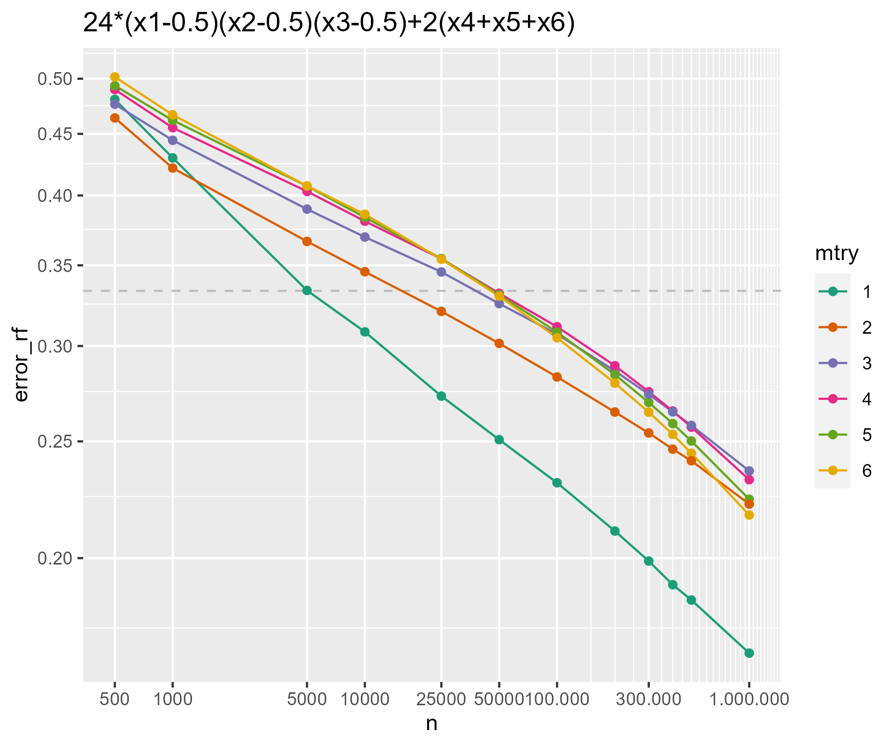
Figure 7: Estimated mean squared error using Random Forest plotted at $\log$-scales for different sample sizes $n$, for the regression model $Y=24(X_{1}-0.5)(X_{2}-0.5)(X_{3}-0.5)+2(X_{4}+X_{5}+X_{6})+\varepsilon$ with $(X_{1},\dots,X_{6})$ uniform on $[0,1]^{6}$ and $\varepsilon\sim\mathcal{N}(0,1)$. The number of trees was set to $100$ and node size was set to $5$. For each sample size, $100$ simulations were carried out. The horizontal dashed line is at $1/3$ which is the mean squared error when using $\hat{m}(X_{1},\dots,X_{6})=2(X_{2}+X_{3}+X_{4})$ as an estimator.

Appendix D Appendix to simulation section

In this section, we provide additional simulation results and collect further details on the simulation results presented in the main text.

D.1 Additional simulation results for different mtrymode

We also performed simulations for RSRF with mtrymode set to fixed and refer to this setup as RSRF (af). The difference between the two versions of RSRF is that for RSRF (af), the covariates where splits are allowed to be placed (in a Random-CART-step) are fixed among the candidate partitions, see Section B.1.1 for details. The setting and results in this case are collected in tables 6, 7 and 14. Interestingly, there is not a big difference between the results for RSRF (af) and RSRF.

Algorithm	Parameter	Value / Range
RSRF (af)	include_cartcart	True, False
	replace	True, False
	width	$1,2,\dots,15\ (d=4,10)$ resp. $1,2,\dots,30\ (d=30)$
	mtry_rsrf_step_random	$1,2,\dots,d$
	mtry_rsrf_step	$1,2,\dots,d$
	min_nodesize	$5,6,\dots,30$
	num_trees	$100$
	mtrymode	fixed

Table 6: Parameter settings for RSRF (af).

Model	Algorithm	$d=4$	$d=10$	$d=30$
	RSRF(opt)	$0.201\ (0.028)$	$0.261\ (0.037)$	$0.369\ (0.062)$
(pure-type)	RSRF (af)(opt)	$0.201\ (0.028)$	$0.279\ (0.040)$	$0.379\ (0.068)$
	INTF(opt)	$0.160\ (0.024)$	$0.220\ (0.030)$	$0.317\ (0.054)$
	RF(opt)	$0.311\ (0.069)$	$0.698\ (0.203)$	$1.336\ (0.292)$
	ET(opt)	$0.207\ (0.048)$	$0.403\ (0.148)$	$0.869\ (0.407)$
	RSRF(opt)	$0.422\ (0.045)$	$0.538\ (0.063)$	$0.674\ (0.067)$
(hierarchical)	RSRF (af)(opt)	$0.417\ (0.044)$	$0.548\ (0.064)$	$0.690\ (0.069)$
	INTF(opt)	$0.383\ (0.042)$	$0.512\ (0.058)$	$0.624\ (0.062)$
	RF(opt)	$0.416\ (0.050)$	$0.554\ (0.066)$	$0.675\ (0.069)$
	ET(opt)	$0.354\ (0.042)$	$0.449\ (0.053)$	$0.531\ (0.059)$
	RSRF(opt)	$0.361\ (0.039)$	$0.460\ (0.053)$	$0.571\ (0.053)$
(additive)	RSRF (af)(opt)	$0.358\ (0.041)$	$0.469\ (0.053)$	$0.576\ (0.055)$
	INTF(opt)	$0.336\ (0.038)$	$0.420\ (0.047)$	$0.502\ (0.048)$
	RF(opt)	$0.343\ (0.039)$	$0.458\ (0.050)$	$0.551\ (0.053)$
	ET(opt)	$0.293\ (0.033)$	$0.366\ (0.046)$	$0.423\ (0.045)$
	RSRF(opt)	$0.148\ (0.026)$	$0.191\ (0.021)$	$0.219\ (0.023)$
(pure-2)	RSRF (af)(opt)	$0.145\ (0.022)$	$0.192\ (0.020)$	$0.222\ (0.022)$
	INTF(opt)	$0.112\ (0.018)$	$0.168\ (0.023)$	$0.207\ (0.020)$
	RF(opt)	$0.184\ (0.025)$	$0.231\ (0.021)$	$0.245\ (0.022)$
	ET(opt)	$0.116\ (0.019)$	$0.187\ (0.018)$	$0.210\ (0.019)$

Model	Algorithm	$d=6$
	RSRF(opt)	$0.195\ (0.032)$
(pure-3)	RSRF (af)(opt)	$0.190\ (0.030)$
	INTF(opt)	$0.151\ (0.028)$
	RF(opt)	$0.518\ (0.063)$
	ET(opt)	$0.429\ (0.041)$

Table 7: Reported mean squared error estimates for different simulations. Standard deviations are provided in brackets.

Model	(pure-type)			(hierarchical)
Dimension $d$	$4$	$10$	$30$	$4$	$10$	$30$
First	INTF	INTF	INTF	ET	ET	ET
Second	RSRF (af)	RSRF	RSRF	INTF	INTF	INTF
Third	RSRF	RSRF (af)	RSRF (af)	RSRF (af)	RSRF	RF
Fourth	ET	ET	ET	RF	RSRF (af)	RSRF
Fifth	RF	RF	RF	RSRF	RF	RSRF (af)

Model	(additive)			(pure-2)
Dimension $d$	$4$	$10$	$30$	$4$	$10$	$30$
First	ET	ET	ET	INTF	INTF	INTF
Second	INTF	INTF	INTF	ET	ET	ET
Third	RF	RF	RF	RSRF	RSRF	RSRF
Fourth	RSRF (af)	RSRF	RSRF	RSRF (af)	RSRF (af)	RSRF (af)
Fifth	RSRF	RSRF (af)	RSRF (af)	RF	RF	RF

Model	(pure-3)
Dimension $d$	$d=6$
First	INTF
Second	RSRF (af)
Third	RSRF
Fourth	ET
Fifth	RF

Table 8: Rankings for (opt).

D.2 Optimal parameters chosen

Tables 10, 9, 11, 13 and 12 contain the optimal parameters found during the parameter search.

	(pure-type)			(hierarchical)
	$d=4$	$d=10$	$d=30$	$d=4$	$d=10$	$d=30$
include_cartcart	FALSE	TRUE	TRUE	FALSE	TRUE	TRUE
replace	TRUE	TRUE	TRUE	FALSE	FALSE	TRUE
width	15	15	30	12	14	29
mtry_cart_cart	-	6	22	-	7	23
mtry_rsrf_step	3	9	30	2	10	26
min_nodesize	16	10	5	5	12	15

	(additive)			(pure-2)
	$d=4$	$d=10$	$d=30$	$d=4$	$d=10$	$d=30$
include_cartcart	FALSE	TRUE	TRUE	FALSE	FALSE	FALSE
replace	TRUE	TRUE	TRUE	TRUE	TRUE	FALSE
width	12	15	16	13	15	25
mtry_cart_cart	-	2	24	-	-	-
mtry_rsrf_step	2	8	24	4	10	30
min_nodesize	14	11	8	23	13	22

	(pure-3)
	$d=6$
include_cartcart	FALSE
replace	TRUE
width	9
mtry_cart_cart	-
mtry_rsrf_step	4
min_nodesize	5

Table 9: Parameters used for RSRF(opt).

	(pure-type)			(hierarchical)
	$d=4$	$d=10$	$d=30$	$d=4$	$d=10$	$d=30$
include_cartcart	FALSE	TRUE	TRUE	FALSE	TRUE	TRUE
replace	TRUE	TRUE	FALSE	TRUE	TRUE	FALSE
width	8	12	28	11	14	24
mtry_rsrf_step_random	3	9	26	4	8	19
mtry_rsrf_step	4	8	26	3	9	30
min_nodesize	14	5	6	10	11	17

	(additive)			(pure-2)
	$d=4$	$d=10$	$d=30$	$d=4$	$d=10$	$d=30$
include_cartcart	FALSE	FALSE	TRUE	FALSE	FALSE	FALSE
replace	TRUE	TRUE	TRUE	TRUE	FALSE	TRUE
width	14	12	12	3	13	24
mtry_rsrf_step_random	4	9	22	4	8	24
mtry_rsrf_step	2	10	26	2	10	28
min_nodesize	12	7	30	20	13	29

	(pure-3)
	$d=6$
include_cartcart	FALSE
replace	FALSE
width	15
mtry_rsrf_step_random	5
mtry_rsrf_step	4
min_nodesize	9

Table 10: Parameters used for RSRF (af)(opt).

	(pure-type)			(hierarchical)
	$d=4$	$d=10$	$d=30$	$d=4$	$d=10$	$d=30$
npairs	14	153	749	7	110	450
replace	TRUE	FALSE	FALSE	FALSE	FALSE	FALSE
min.node.size	20	11	11	10	8	17

	(additive)			(pure-2)
	$d=4$	$d=10$	$d=30$	$d=4$	$d=10$	$d=30$
npairs	23	33	99	2	151	30
replace	TRUE	FALSE	FALSE	FALSE	FALSE	FALSE
min.node.size	13	14	18	16	26	28

	(pure-3)
	$d=6$
npairs	99
replace	TRUE
min.node.size	22

Table 11: Parameters used for INTF(opt).

	(pure-type)			(hierarchical)
	$d=4$	$d=10$	$d=30$	$d=4$	$d=10$	$d=30$
mtry	4	10	30	3	6	9
replace	TRUE	FALSE	FALSE	TRUE	TRUE	TRUE
min.node.size	5	5	7	8	6	12

	(additive)			(pure-2)
	$d=4$	$d=10$	$d=30$	$d=4$	$d=10$	$d=30$
mtry	2	7	26	2	5	20
replace	TRUE	TRUE	TRUE	TRUE	TRUE	TRUE
min.node.size	5	15	18	10	8	30

	(pure-3)
	$d=6$
mtry	5
replace	TRUE
min.node.size	6

Table 12: Parameters used for RF(opt).

	(pure-type)			(hierarchical)
	$d=4$	$d=10$	$d=30$	$d=4$	$d=10$	$d=30$
mtry	4	9	29	3	9	29
num.random.splits	3	3	6	3	3	9
replace	FALSE	FALSE	FALSE	FALSE	FALSE	FALSE
min.node.size	12	5	5	8	5	9

	(additive)			(pure-2)
	$d=4$	$d=10$	$d=30$	$d=4$	$d=10$	$d=30$
mtry	3	7	29	2	7	28
num.random.splits	5	3	3	1	1	1
replace	TRUE	FALSE	FALSE	FALSE	TRUE	TRUE
min.node.size	6	10	16	10	6	15

	(pure-3)
	$d=6$
mtry	1
num.random.splits	5
replace	FALSE
min.node.size	5

Table 13: Parameters used for ET(opt).

D.3 Some remarks on the parameters in RSRF

Below, we include some remarks on the parameter choices for RSRF. Nonetheless, we want to point out that this discussion should be considered as heuristic and a deeper analysis on how to choose the hyper-parameters is beyond the scope of this paper. The width parameter $0pt$ is the most important tuning parameter in RSRF. From our simulations we see that best results were usually obtained for large choices of $0pt$. However, a closer look at the tables in the supplementary material reveals that, for the pure interaction models, RSRF improves upon Random Forests also for small values of $0pt$. For instance, in (pure-3), choosing a small $0pt=3$ for RSRF (af) already achieved an MSE of $\approx 0.25$ whereas the error for RF is larger than $0.5$ (see Figure 2). Furthermore, it is important to tune the mtry-parameters. We note that, in order to reduce the number of tuning parameters, one could instead consider a single mtry parameter by setting $\texttt{mtry\_cart\_cart}=\texttt{mtry\_random\_cart}$ for RSRF (af), and similarly for RSRF. Motivated from our simulations, we do not believe that the node size is particularly important and suggest it to choose rather small, e.g. $10$. Lastly, let us briefly discuss the parameter include_cartcart. We observe that for large $d=30$ in models (hierarchical), (additive), it is advantageous to set this parameter to “true” (this was the case in almost all of the top $20$ parameter setups for both RSRF, RSRF (af)). Contrary, in the pure model (pure-2) for RSRF (af), it was set to “false” in $15$ out of the top $20$ setups (and in $19$ out of the top $20$ settings in (pure-type) with $d=30$). We note that the choice for include_cartcart should also be connected to the width parameter $0pt$. The larger the width, the less influential is include_cartcart.

Model	Algorithm	$d=4$	$d=10$	$d=30$	$d=6$
(pure-type)	RSRF (af)(CV)	$0.212\ (0.034)$	$0.272\ (0.039)$	$0.401\ (0.075)$	$-$
(hierarchical)	RSRF (af)(CV)	$0.428\ (0.050)$	$0.561\ (0.067)$	$0.689\ (0.074)$	$-$
(additive)	RSRF (af)(CV)	$0.375\ (0.043)$	$0.492\ (0.061)$	$0.585\ (0.053)$	$-$
(pure-2)	RSRF (af)(CV)	$0.152\ (0.025)$	$0.198\ (0.021)$	$0.230\ (0.025)$	$-$
(pure-3)	RSRF (af)(CV)	$-$	$-$	$-$	$0.192\ (0.030)$

Table 14: Reported mean squared error estimates for different simulations. Standard deviations are provided in brackets.

References

- [1] Sumanta Basu, Karl Kumbier, James B Brown, and Bin Yu. Iterative random forests to discover predictive and stable high-order interactions. Proceedings of the National Academy of Sciences, 115(8):1943–1948, 2018.
- [2] Gérard Biau and Erwan Scornet. A random forest guided tour. TEST, 25:197–227, 2016.
- [3] Ricardo Blum, Munir Hiabu, Enno Mammen, and Joseph Theo Meyer. Consistency of random forest type algorithms under a probabilistic impurity decrease condition. arXiv preprint arXiv:2309.01460v2, 2024.
- [4] Leo Breiman. Random forests. Machine Learning, 45(1):5–32, 2001.
- [5] Leo Breiman, Jerome Friedman, Charles J. Stone, and R.A. Olshen. Classification and Regression Trees. Chapman and Hall/CRC, 1984.
- [6] Chien-Ming Chi, Patrick Vossler, Yingying Fan, and Jinchi Lv. Asymptotic properties of high-dimensional random forests. The Annals of Statistics, 50(6):3415 – 3438, 2022.
- [7] Hugh A. Chipman, Edward I. George, and Robert E. McCulloch. BART: Bayesian additive regression trees. The Annals of Applied Statistics, 4(1):266 – 298, 2010.
- [8] Stéphan Clémençon, Marine Depecker, and Nicolas Vayatis. Ranking forests. The Journal of Machine Learning Research, 14(1):39–73, 2013.
- [9] Antonio Criminisi, Duncan Robertson, Ender Konukoglu, Jamie Shotton, Sayan Pathak, Steve White, and Khan Siddiqui. Regression forests for efficient anatomy detection and localization in computed tomography scans. Medical image analysis, 17(8):1293–1303, 2013.
- [10] Antonio Criminisi, Jamie Shotton, Ender Konukoglu, et al. Decision forests: A unified framework for classification, regression, density estimation, manifold learning and semi-supervised learning. Foundations and trends in computer graphics and vision, 7(2–3):81–227, 2012.
- [11] Ramón Díaz-Uriarte and Sara Alvarez de Andrés. Gene selection and classification of microarray data using random forest. BMC bioinformatics, 7:1–13, 2006.
- [12] Pierre Geurts, Damien Ernst, and Louis Wehenkel. Extremely randomized trees. Machine Learning, 63:3–42, 04 2006.
- [13] Shihao Gu, Bryan Kelly, and Dacheng Xiu. Empirical asset pricing via machine learning. The Review of Financial Studies, 33(5):2223–2273, 2020.
- [14] Munir Hiabu, Enno Mammen, and Joseph T. Meyer. Random Planted Forest: a directly interpretable tree ensemble. arXiv e-prints, page arXiv:2012.14563, December 2020.
- [15] Giles Hooker. Generalized functional ANOVA diagnostics for high-dimensional functions of dependent variables. Journal of Computational and Graphical Statistics, 16(3):709–732, 2007.
- [16] Roman Hornung. Diversity forests: Using split sampling to enable innovative complex split procedures in random forests. SN computer science, 3:1–16, 2022.
- [17] Roman Hornung and Anne-Laure Boulesteix. Interaction forests: Identifying and exploiting interpretable quantitative and qualitative interaction effects. Computational Statistics & Data Analysis, 171:107460, 2022.
- [18] Hemant Ishwaran, Udaya B Kogalur, Eugene H Blackstone, and Michael S Lauer. Random survival forests. The Annals of Applied Statistics, 2(3):841 – 860, 2008.
- [19] Jason M. Klusowski and Peter M. Tian. Large scale prediction with decision trees. Journal of American Statistical Association, 2022.
- [20] Rahul Mazumder and Haoyue Wang. On the convergence of cart under sufficient impurity decrease condition. In A. Oh, T. Neumann, A. Globerson, K. Saenko, M. Hardt, and S. Levine, editors, Advances in Neural Information Processing Systems, volume 36, pages 57754–57782. Curran Associates, Inc., 2023.
- [21] Nicolai Meinshausen. Quantile regression forests. Journal of machine learning research, 7(6), 2006.
- [22] Jens Perch Nielsen and Stefan Sperlich. Smooth backfitting in practice. Journal of the Royal Statistical Society. Series B (Statistical Methodology), 67(1):43–61, 2005.
- [23] Yanjun Qi. Random forest for bioinformatics. Ensemble machine learning: Methods and applications, pages 307–323, 2012.
- [24] Charles J Stone. The use of polynomial splines and their tensor products in multivariate function estimation. Annals of Statistics, 22(1):118–171, 1994.
- [25] Vasilis Syrgkanis and Manolis Zampetakis. Estimation and inference with trees and forests in high dimensions. In Jacob Abernethy and Shivani Agarwal, editors, Proceedings of Thirty Third Conference on Learning Theory, volume 125 of Proceedings of Machine Learning Research, pages 3453–3454. PMLR, 09–12 Jul 2020.
- [26] Stefan Wager and Susan Athey. Estimation and inference of heterogeneous treatment effects using random forests. Journal of the American Statistical Association, 113(523):1228–1242, 2018.
- [27] Marvin N. Wright and Andreas Ziegler. ranger: A fast implementation of random forests for high dimensional data in c++ and r. Journal of Statistical Software, 77(1):1–17, 2017.
- [28] Marvin N Wright, Andreas Ziegler, and Inke R König. Do little interactions get lost in dark random forests? BMC bioinformatics, 17:1–10, 2016.