Rate of epidemic spreading on complex networks
Abstract
The initial phase of an epidemic is often characterised by an exponential increase in the number of infected individuals. In a well-mixed population, this exponential increase is controlled by the basic reproduction number and the distribution of times between consecutive infection along an infection chain. However, real populations are characterised by a complex network of interactions, and are thus far from being well mixed. Here, we derive an expression for the rate of exponential spread of an epidemic on a complex network. We find that this rate is affected by the degree distribution, the network assortativity, and the level of clustering. Our result holds for a broad range of networks, apart from networks with very broad degree distribution, where no clear exponential regime is present. The theory presented in this paper bridges the gap between classic epidemiology and the theory of complex network, with broad implications for model inference and policy making.
Epidemic modelling permits rationalisation of evidences and can provide crucial information for policy making. Epidemiological models should incorporate the key features that determine epidemic spreading. One such feature is the arrangement of individuals in social structures [1]. These social structures play a crucial role in the spreading of an epidemic, and in the effectiveness of intervention strategies [2, 3]. In these social structures, the number of contacts per individual is highly variable. For example, at the early stages of COVID-19, the individuals with most contacts contributed disproportionately to the epidemic [4, 5].
A convenient way of modelling social structures is by means of complex networks [6], in which nodes represent individuals and links signify pairs of individuals that are in close contact. A success of network theory has been to determine the epidemic threshold on networks [7, 8, 9], i.e., the transition point from a localised outbreak to a widespread epidemic. This theory has shown that networks whose degree distribution has a diverging variance due to heavy tails [7, 10, 9] are extremely vulnerable to epidemics. A paradigmatic example is found in the Barabási-Albert model [11], where a network is constructed by preferentially attaching new nodes to existing nodes with high degree. Another property of complex networks which is relevant for epidemic spreading is clustering, which is a measure of how commonly nodes tend to form tightly connected communities. Many networks in nature possess both fat tails in their degree distribution and high level of clustering [12].
Another key feature of an epidemic is its infectiousness, i.e., the rate at which an infected individual infects its contacts. The infectiousness incorporates multiple factors, such as the viral load of an individual, its social behaviour, and possibly environmental factors [13]. Because of changes in these factors, the infectiousness of an individual tends to change in time in a way that is particular to each disease. This time-dependence profoundly impacts the way a disease spreads.
Social structures and individual infectiousness are the key factors in determining the initial stage of an epidemic, in which most individuals are susceptible and the number of infected individuals usually grows exponentially. This stage is of central importance for novel epidemics, or during emergence of novel variants, and it often requires rapid policy making. At later stages, other factors become relevant, such as individual recovery time, their behavioural change as a consequence of the epidemic [14], and the possible occurrence of reinfections.
Despite the vast body of theory on epidemics in networks [9], general results on the speed of epidemic spreading are surprisingly sparse. The rate of epidemic spreading can be calculated for unclustered, uncorrelated networks, and with constant infectiousness [15]. A recent theory estimates the average time it takes for an epidemic to reach an individual at a certain distance from patient zero [16]. The spread of an epidemic on a network can be exactly solved [17], but this calculation becomes practically unfeasible unless the network is very small. Other approaches avoid a detailed description of social structures, and effectively model the heterogeneity of the population by assigning different risk propensities to individuals [18, 19].
In this paper, we present a general theory that predicts the exponential rate of epidemic spreading on a complex network. In particular, we quantify the impact of key properties of the network, such as assortativity and clustering, on the reproduction number of the epidemic. We further link the reproduction number and the individual infectiousness with the epidemic spreading rate. We shall see that this approach leads to accurate predictions for a broad range of networks.
Epidemic spreading in well-mixed populations
We begin by summarising classic results of epidemic modelling in well-mixed populations [13]. In this case, the cumulative number of infected individuals at time is governed by the renewal equation
| (1) |
where the basic reproduction number represents the average number of secondary infections by each infected individual, and the dot denotes a time derivative. The function is the infectiousness, defined as the probability density that a given secondary infection occurs after a time from the primary one. We assume to be in the exponential regime, , where is the rate of exponential spread. Substituting this assumption into Eq. (1) and taking the limit of large time, we obtain the Euler-Lotka equation
| (2) |
where the average is over the distribution . Equation (2) is a cornerstone in mathematical epidemiology, as it provides a fundamental link between the three key quantities governing the epidemic spreading: the distribution of infection times ; the basic reproduction number ; and the exponential spreading rate .
Epidemic spreading in networks.
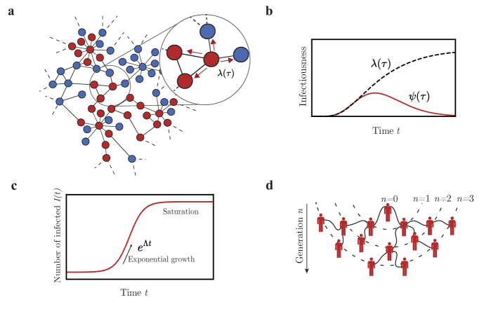
We now consider a structured population composed of individuals, who are represented as nodes on a network (Fig. 1a). Two individuals are connected by a link if they are in contact, meaning that they can potentially infect one another. Once an individual is infected, it can spread the disease to each of its neighbours at rate , where is the time since the considered individual was infected. The probability that the individual infects a given neighbour at time , given that the neighbour has not been infected before by someone else, is then equal to . We call the generation time distribution (Fig. 1b). The integral represents the total probability of infecting a susceptible neighbour. Aside from this normalisation, the generation time distribution plays the role of the distribution for well-mixed systems. In the following, we focus for simplicity on the case . In this case, individuals infect all of their contacts and the epidemic eventually spreads through all the network, if the network is connected. Our results can be extended to the case by randomly removing links in the networks (see Section LABEL:SI-sec:p_psi in SI).
Infected nodes cannot get reinfected and are never formally considered as recovered, although their infectiousness may wane over time. Our model can therefore be seen as a Susceptible-Infected model on a network with non-Markovian infection times. The Markov property only holds in the limiting case of constant , and consequently exponentially distributed . This limiting case is often unrealistic. For example, the infectiousness of COVID-19 markedly increases for 3–6 days and then decay for about 11 days [20], and is therefore poorly described by an exponential distribution.
In the course of the epidemic, the number of infected rapidly grows before saturating (Fig. 1c). An alternative to the temporal perspective is to represent the epidemic in generations (Fig. 1d). We call , the average number of infected individuals in the th generation. The initial generation, , is constituted by the patient zero, . In this representation, the infected individuals form a tree (Fig. 1e).
Reproduction number on a complex network
The basic reproduction number for a network is the average number of links of an infected individual in the early stage of the epidemic, excluding the one from which the infection came from. We also define the effective reproduction number as the average number of infections caused by an infected individual. In contrast with , does not include contacts that are infected by other individuals. This difference is crucial in clustered networks.
Our initial goal is to estimate for a complex network. To this aim, we characterise individuals by their degree . We introduce the reproduction matrix , whose elements are the average numbers of susceptible individuals of degree connected to a node of degree . The reproduction matrix is expressed by
| (3) |
where is the probability that a neighbour of a node of degree has degree and is the average number of triangles a -link is part of. The term proportional to in Eq. (3) discounts for contacts of a given individual that were already infected by someone else, due to the presence of triangles in the network. In Eq. (3), we neglect higher order loops such as squares. The reproductive matrix given in Eq. (3) has been used to study percolation on networks [21].
On the one hand, assuming that remains constant between generations, the average number of infected individuals at the th generation is equal to , up to the leading order. On the other hand, the number of infected individuals scales as the -th power of the reproduction matrix (see Methods). This permits us to identify as the leading eigenvalue of the reproduction matrix. The associated right eigenvector can be interpreted as the degree distribution of the infected individuals (see Methods).
For large networks, diagonalising the reproduction matrix can be unwieldy. In the simple case of an unclustered network for all links) in which the degrees of connected nodes are uncorrelated, we have
| (4) |
where the bar represents an average over the degree distribution. Equation (4) is a classic result for epidemic spreading on networks [7, 22, 8]. We seek to extend it to the general case of clustered and correlated networks. We quantify degree correlations by the assortativity coefficient (see Methods). When , nodes with high degree tend to connect together whereas when , they tend to connect to lower degree nodes. We find that, for small clustering coefficients and degree correlation, the effective reproduction number is expressed by
| (5) |
where is the probability that two neighbours of a node of degree are themselves connected, is the average number of triangles a link is part of, and . Equation (5) is obtained by a perturbative expansion in (see Methods).
We compare the expression for given in Eq. (5) to the maximum eigenvalue of the matrix for different network models, see Table 1. We find that the relative difference between and is within for all the networks we considered, except for Barabási-Albert with () and (). We shall analyse the reason for this discrepancy later in the paper. Approximating with given in Eq. (4) leads to substantially larger errors, supporting that clustering and assortativity need to be taken into account to appropriately estimate . Here and in the following, when computing using Eq. (5) and using Eq. (4) for a given network, we always interpret the averages as empirical averages. With this choice, moments of the degree distribution are always finite, even in very heterogeneous networks. In practical cases, Eq. (5) predicts that the reproduction number increases with the assortativity . Accordingly, assortativity lowers the epidemic threshold, as previously known for the unclustered case [23]. However, the coefficient multiplying in Eq. (5) is usually rather small, except when the degree distribution has heavy tails. In contrast, clustering systematically reduces , regardless of the degree distribution. For this reason, we find that overestimates in all the synthetic networks we considered.
| Network | Assortativity | Clustering | |||||
|---|---|---|---|---|---|---|---|
| 13.9 | 8.5 | 6.8 | 13.9 | 6.6 | -0.011 | 0 | |
| 20.4 | 15.5 | 14.4 | 20.3 | 14.2 | -0.008 | 0.0001 | |
| 85.4 | 80.8 | 79.5 | 83.6 | 80.4 | -0.004 | 0.0003 | |
| 6.0 | 6.0 | 6.0 | 6.0 | 6.0 | 0.001 | 0.000 | |
| 10.0 | 9.0 | 9.1 | 9.0 | 10.7 | 0.062 | 0.108 | |
| 7.2 | 4.9 | 4.9 | 4.9 | 7.0 | -0.022 | 0.334 | |
| 5.2 | 3.6 | 3.6 | 3.6 | 5.0 | -0.029 | 0.315 | |
| 3.7 | 3.2 | 3.2 | 3.2 | 3.8 | 0.007 | 0.161 |
Network Euler-Lotka equation
We now use our estimate of the reproduction number to predict how epidemics spread. The average total number of infected individual of degree at time is governed by the renewal equation
| (6) |
Equation (6) extends Eq. (1) to complex networks. It is linear because of the assumption that the epidemic is in the initial stage and thus far from saturation. We assume exponential growth, . Substituting this assumption into Eq. (6) we obtain, for large time,
| (7) |
where denotes an average over . We call Eq. (7) the network Euler-Lotka equation (see Section LABEL:SI-sec:LDP in SI for an alternative derivation). Although the course of infectiousness and the network topology conspire in determining the spreading rate , these two aspects appear as separated in Eq. (7). Indeed, the right hand side of Eq. (7) only depends on at given , while the left hand side is uniquely determined by the network topology. This latter fact depends on having fixed ; otherwise, would have depended on as well (see Section LABEL:SI-sec:p_psi in SI). Equation (7) predicts that the epidemic threshold, i.e the condition , is obtained by setting , independently of .
In general, we shall use Eq. (7) as an implicit relation for the unknown . It is possible to explicitly express from Eq. (7), but only in an approximate way. In particular, using the first two moments of the generation-time distribution, we obtain
| (8) |
where , see Section LABEL:SI-gaussian in SI. An alternative is to combine Eq. (7) with the Jensen inequality, that states that . This leads to a lower bound on the exponential spreading rate of the epidemic:
| (9) |
The bound in Eq. (9) is saturated when the epidemic spreads at regular time interval, i.e., when is a Dirac delta function.
Synthetic networks
The network Euler-Lotka equation successfully predicts the rate of epidemic spreading on synthetic complex networks, Fig. 2-a and Fig. 2-b. Our battery of tests includes a broad range of models characterised by different degree distribution, assortativity, and clustering. For each model, we ran simulations using three different infectivity functions, see Fig. 2-c. The choice of the infectivity function qualitatively affect the behaviour of the epidemic. In particular, for peaked distributions, the exponential growth appears modulated by oscillations (Fig. 2-a), since early generations of the epidemic are nearly synchronised. To extrapolate the leading exponential behaviour from these curves, we fit them to a generalised logistic function, which appear to well capture finite-size effects (see Methods). The fits also permits to define a finite-size parameter , which quantifies the relative impact of finite-size effects on the exponential spreading rate at short times (see Methods and Section LABEL:SI-sec:eta in SI). When predicting the exponential growth rate using the network Euler-Lotka equation, we use as defined in Eq. (5) as the reproduction number. As expected, the predictions are considerably worse if we instead use , see Section LABEL:SI-sec:R_vs_R0 in SI. The difference between the exponential spreading rate estimated from the simulations and from the network Euler-Lotka equation (7) is within for all networks, see Fig. 2-c. The only exception is the Barabási-Albert network with parameter (average error ), where represents the number of nodes a new node attaches to.
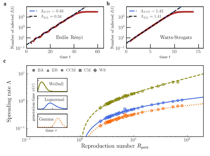
There are two causes for this exception. The first is that the exponential regime for this model is not clearly defined, as revealed by the finite-size parameter (see Fig. 2). This issue is likely related with the fact that the second moment of the degree distribution diverges in the infinite size limit. The second cause is that, for , the first-order perturbative expansion in loses accuracy, as revealed by the difference between and the leading eigenvalue of the reproductive matrix (see Table 1).
Real-world networks
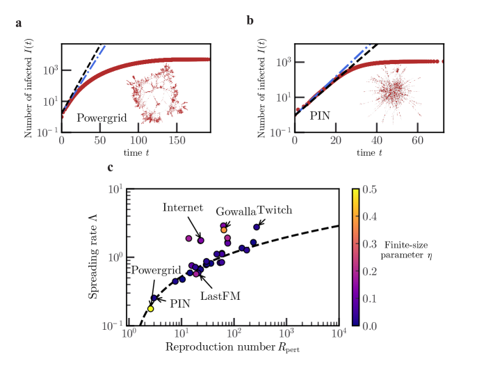
We apply the network Euler-Lotka equation to a large set of social, biological, technological, and transportation networks, see Fig. 3. These real-world networks exhibit more complex structures than synthetic networks. They are often characterised by tightly linked communities, strong degree-correlation and broad tails in the degree distribution. Therefore, they constitute a more challenging test. Nevertheless, the network Euler-Lotka equation holds well, see Fig. 3-a and Fig. 3-b for examples.
More generally, we find that the prediction of the network Euler-Lotka equation well reproduces the fitted spreading rate whenever the finite-size parameter detects a clear exponential regime, see Fig. 3-c. Although some of these networks are highly clustered, using as expressed by Eq. (5) does not perform worse than (See Section LABEL:SI-sec:R_vs_R0 in SI). In Fig. 3-c, we have omitted three road networks (California, Texas, and Pennsylvania). For these networks, the generalised logistic fit fails to converge. However, a function of the form well fits the epidemic trajectories on these networks (see Section LABEL:SI-power-law-fit in SI). Likely, the fact that these networks are embedded in a two-dimensional physical space prevents an exponential epidemic spread.
For networks in which our fit detects small finite-size effects (), the predictions of the network Euler-Lotka equation using are more accurate than those using . However, for larger values of , performs slightly better on average (see Section LABEL:SI-sec:R_vs_R0 in SI). Even in these cases, provides a better approximation of the reproduction number , see SI Fig. LABEL:SI-fig:Rpert_vs_eta-b. This suggests that the advantage of for large might be due to a compensatory effect: using tends to overestimate the reproduction number, while the network Euler-Lotka equation tends to underestimate compared to .
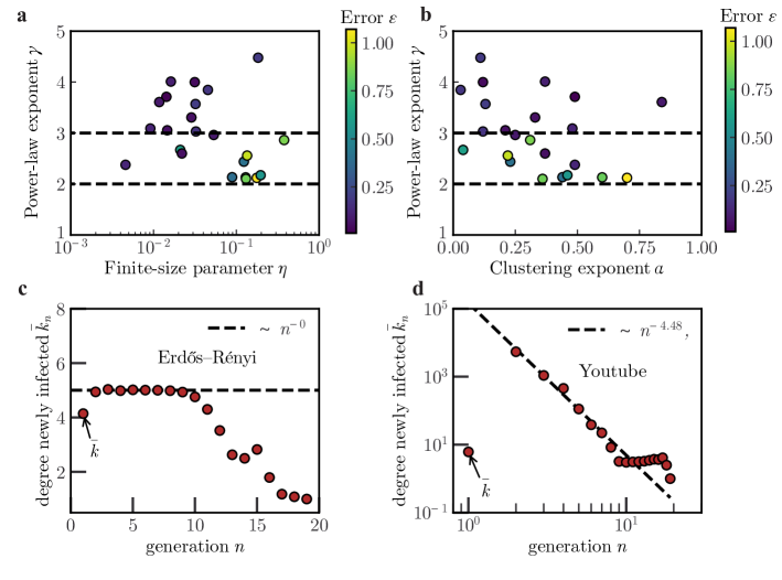
We aim at understanding why, for certain real-world networks, the predicted spreading rate deviates from the fitted one. We find large errors only for scale-free networks in which the finite-size parameter is also large, see Fig. 4-a. We call a network scale-free if the tail of its degree distribution are fitted by a power law of the form , with , multiplied by a slowly varying function, see [28] and Section LABEL:SI-sec:tail in SI. In contrast, the error is weakly affected by the strength of clustering, see Fig. 4-b. One issue with heavy-tailed networks is that the rapid infection of hubs depletes the tail of the degree distribution of the remaining nodes. This implies that, as the epidemic progresses, the degree distribution of the infected nodes does not remain invariant as assumed by our theory. To test this explanation, we study the average degree of infected individuals in generation . In a steady exponential regime, we expect this quantity to be independent of , see Fig. 4-c. However, in scale-free networks, the average degree of infected individuals appears to decay as a power-law of their generation, see Fig. 4-d, leading to a non-steady spreading.
Discussion
In this paper, we developed a theory describing the exponential spreading rate of epidemics in populations arranged on a complex network. Our theory relates the spreading rate to the infectiousness and the social structure, while disentangling the impact of their distinct properties. Our approach accurately predicts the spreading rate on a wide range of model and real networks, aside from networks with heavy-tailed degree distributions where the exponential regime is hindered by finite-size effects.
When analysing the early stage of real epidemics, a departure from an exponential behaviour in the observed number of cases is often interpreted as a consequence of individual response or early containment measures (see, e.g., [29]). Our results show that non-exponential epidemic trajectories are common in heavy-tailed networks, thus providing an alternative explanation for these observations.
The theory developed in this paper can be also used to estimate the basic reproduction number [30]. Ideally, in the early stage of an epidemic, one could use the Euler-Lotka equation to deduce . However, this approach is fraught with practical difficulties. First, the curves in Fig. 2f show that a small error in the estimate of the exponential spreading rate can lead to a large uncertainty on . Second, it is often difficult to reliably estimate the infectiousness distribution (see, e.g., [31, 32, 33] for the case of COVID-19). Instead, our theory permits to directly estimate from structural properties of the interaction networks, such as moments of the degree distribution and clustering. These properties could be inferred, to some extent, based on contact tracing data [34]. As a consequence, such approach could lead to improved estimates of the infectivity function as well.
We have focused for simplicity on static networks, which is justified when the social structures evolve in a slower way than the time scale of the infection process. If however the time-scales are similar, epidemic dynamics are more complex [35]. For example, bursty social interactions substantially affect epidemic spreading [36]. In principle, interactions could be also weighted, as duration and intensity of contacts affect the probability of transmission [37]. The approach developed in this paper is flexible enough to be extended to these scenarios.
Methods
Reproduction Number
We here derive the expression for the reproduction number, Eq. (5). We express the average number of infected individuals at generation in terms of the reproduction matrix introduced in Eq. (3) by summing over the degree of individuals at each generation:
| (10) |
At the first generation, we obtain . For large , we have , where is the leading eigenvalue of . For an arbitrary level of clustering and of degree correlation, the leading eigenvalue is not easy to compute exactly. We therefore approximate the eigenvalue by assuming weak clustering and treating the degree correlations as a perturbation of the uncorrelated case.
Degree correlations are summarised by the assortativity [38], defined as the Pearson correlation coefficient of the degrees of connected nodes:
| (11) |
where ensures that and is the probability that a randomly chosen edge connects nodes of degrees and .
We now analyse the clustering measure . While being a measure of clustering, also contains information on the degree correlation of connected nodes. In contrast, the degree dependent clustering coefficient is independent of degree correlations [39]. This coefficient is related to as . If we assume that factorises into and -dependent factors, we can express as
| (12) |
where . In particular, this factorisation is justified in the weak clustering limit [39]. Using this expression, we rewrite the reproduction matrix as
| (13) |
To further simplify the problem, we neglect the dependence on of the probability that a node of degree connected to a node of degree is part of a triangle. This amounts to assume , so that Eq. (13) becomes
| (14) |
We now treat as a small perturbation parameter and express the leading eigenvalue using perturbation theory. To this aim, we express the reproduction matrix as
| (15) |
with
| (16) | ||||
| (17) |
where we have used that for and is unspecified, but satisfies and . At this order in perturbation theory, the degrees of connected nodes are linearly correlated.
At the first order in , we obtain
| (18) |
see SI, where we defined . At this order, the right eigenvector associated to the unique leading eigenvalue is given by:
| (19) |
This eigenvector, if normalised, represents the relative probability that an infected individual has degree in the exponential regime.
Spreading rate of simulated epidemics: Generalised Logistic Function
We describe our extrapolation of the exponential spreading rate of an epidemic from simulation data. In networks with heavy tails, finite-size effects alter the course of the epidemic at relatively early times. Likely for this reason, we have observed that functions such as a simple logistic regression fail to fit well the course of the epidemic. In contrast, we have found that the generalised logistic function
| (20) |
well fits the epidemic trajectories for the large majority of networks that we considered. In Eq. (20), the size of the network and where the initial number of infected individuals. Although each simulation starts with a single infected individual, we consider as a free parameter to better capture the behaviour of the epidemic at the early stages. The remaining free parameters are and . We fit the logarithm of the generalised logistic function, and discard the first infection events of each simulation, i.e., the times until . The reason is that these infections should belong to the first generation , in which the average number of secondary infections per individual is rather than .
A linearisation of for small in Eq. (20) shows that:
| (21) |
For , we obtain . Equation (21) leads us to define the finite-size parameter and the finite-size growth rate . For , we recover a classic logistic function, while for the generalised logistic function tends to a Gompertz curve. For the synthetic and real-world networks that we studied, we have found that the finite-size parameter correlates with the curvature of for small , i.e. the deviation from an exponential behaviour (see Section LABEL:SI-sec:eta in SI).
We call the value of that makes Eq. (20) fit best the data. We call the value of obtained as solution of the Euler-Lotka equation. We measure the quality of our predictions by means of the symmetric relative error:
| (22) |
The fits of all epidemic trajectories, together with tables presenting all values of the and are presented in Section LABEL:SI-sec:simulations in SI.
Acknowledgements
We thank C. Castellano and I. Neri for comments on a preliminary version of this manuscript. We thank Joshua Weitz for discussions. We are grateful for the help and support provided by the Scientific Computing and Data Analysis section of Core Facilities at OIST.
References
- [1] Buckee, C., Noor, A. & Sattenspiel, L. Thinking clearly about social aspects of infectious disease transmission. Nature 595, 205–213 (2021).
- [2] Patwardhan, S., Rao, V. K., Fortunato, S. & Radicchi, F. Epidemic spreading in group-structured populations. Physical Review X 13, 041054 (2023).
- [3] Granell, C. & Mucha, P. J. Epidemic spreading in localized environments with recurrent mobility patterns. Physical Review E 97, 052302 (2018).
- [4] Kumar, S., Jha, S. & Rai, S. K. Significance of super spreader events in covid-19. Indian Journal of Public Health 64, 139–141 (2020).
- [5] Sneppen, K., Taylor, R. J. & Simonsen, L. Impact of Superspreaders on dissemination and mitigation of COVID-19. MedRxiv 2020–05 (2020).
- [6] Newman, M. Networks (Oxford university press, 2018).
- [7] Pastor-Satorras, R. & Vespignani, A. Epidemic spreading in scale-free networks. Physical Review Letters 86, 3200 (2001).
- [8] Newman, M. E. Spread of epidemic disease on networks. Physical Review E 66, 016128 (2002).
- [9] Pastor-Satorras, R., Castellano, C., Van Mieghem, P. & Vespignani, A. Epidemic processes in complex networks. Reviews of Modern Physics 87, 925 (2015).
- [10] Barthélemy, M., Barrat, A., Pastor-Satorras, R. & Vespignani, A. Dynamical patterns of epidemic outbreaks in complex heterogeneous networks. Journal of theoretical biology 235, 275–288 (2005).
- [11] Pósfai, M. & Barabási, A.-L. Network Science (Citeseer, 2016).
- [12] Ravasz, E. & Barabási, A.-L. Hierarchical organization in complex networks. Physical Review E 67, 026112 (2003).
- [13] Grassly, N. C. & Fraser, C. Mathematical models of infectious disease transmission. Nature Reviews Microbiology 6, 477–487 (2008).
- [14] Weitz, J. S., Park, S. W., Eksin, C. & Dushoff, J. Awareness-driven behavior changes can shift the shape of epidemics away from peaks and toward plateaus, shoulders, and oscillations. Proceedings of the National Academy of Sciences 117, 32764–32771 (2020).
- [15] Barthélemy, M., Barrat, A., Pastor-Satorras, R. & Vespignani, A. Velocity and hierarchical spread of epidemic outbreaks in scale-free networks. Physical Review Letters 92, 178701 (2004).
- [16] Moore, S. & Rogers, T. Predicting the speed of epidemics spreading in networks. Physical Review Letters 124, 068301 (2020).
- [17] Merbis, W. & Lodato, I. Logistic growth on networks: Exact solutions for the susceptible-infected model. Physical Review E 105, 044303 (2022).
- [18] Rose, C. et al. Heterogeneity in susceptibility dictates the order of epidemic models. Journal of Theoretical Biology 528, 110839 (2021).
- [19] Berestycki, H., Desjardins, B., Weitz, J. S. & Oury, J.-M. Epidemic modeling with heterogeneity and social diffusion. Journal of Mathematical Biology 86, 60 (2023).
- [20] Hakki, S. et al. Onset and window of SARS-CoV-2 infectiousness and temporal correlation with symptom onset: a prospective, longitudinal, community cohort study. The Lancet Respiratory Medicine 10, 1061–1073 (2022).
- [21] Serrano, M. Á. & Boguná, M. Clustering in complex networks. II. Percolation properties. Physical Review E 74, 056115 (2006).
- [22] Callaway, D. S., Newman, M. E., Strogatz, S. H. & Watts, D. J. Network robustness and fragility: Percolation on random graphs. Physical Review Letters 85, 5468 (2000).
- [23] Goltsev, A. V., Dorogovtsev, S. N., Oliveira, J. G. & Mendes, J. F. Localization and spreading of diseases in complex networks. Physical Review Letters 109, 128702 (2012).
- [24] Serrano, M. A. & Boguná, M. Tuning clustering in random networks with arbitrary degree distributions. Physical Review E 72, 036133 (2005).
- [25] Clauset, A., Tucker, E. & Sainz, M. The Colorado Index of Complex Networks. https://icon.colorado.edu/ (2016).
- [26] Leskovec, J. & Krevl, A. SNAP Datasets: Stanford large network dataset collection. http://snap.stanford.edu/data (2014).
- [27] Kunegis, J. KONECT – The Koblenz Network Collection. In Proc. Int. Conf. on World Wide Web Companion, 1343–1350 (2013). URL http://dl.acm.org/citation.cfm?id=2488173.
- [28] Voitalov, I., Van Der Hoorn, P., Van Der Hofstad, R. & Krioukov, D. Scale-free networks well done. Physical Review Research 1, 033034 (2019).
- [29] Maier, B. F. & Brockmann, D. Effective containment explains subexponential growth in recent confirmed COVID-19 cases in China. Science 368, 742–746 (2020).
- [30] Birello, P., Re Fiorentin, M., Wang, B., Colizza, V. & Valdano, E. Estimates of the reproduction ratio from epidemic surveillance may be biased in spatially structured populations. Nature Physics 1–7 (2024).
- [31] Lauer, S. A. et al. The incubation period of coronavirus disease 2019 (COVID-19) from publicly reported confirmed cases: estimation and application. Annals of Internal Medicine 172, 577–582 (2020).
- [32] Ferretti, L. et al. Quantifying SARS-CoV-2 transmission suggests epidemic control with digital contact tracing. Science 368, eabb6936 (2020).
- [33] Nishiura, H., Linton, N. M. & Akhmetzhanov, A. R. Serial interval of novel coronavirus (COVID-19) infections. International Journal of Infectious Diseases 93, 284–286 (2020).
- [34] Kojaku, S., Hébert-Dufresne, L., Mones, E., Lehmann, S. & Ahn, Y.-Y. The effectiveness of backward contact tracing in networks. Nature Physics 17, 652–658 (2021).
- [35] Cai, C.-R., Nie, Y.-Y. & Holme, P. Epidemic criticality in temporal networks. Physical Review Research 6, L022017 (2024).
- [36] Tkachenko, A. V. et al. Stochastic social behavior coupled to COVID-19 dynamics leads to waves, plateaus, and an endemic state. Elife 10, e68341 (2021).
- [37] Ferretti, L. et al. Digital measurement of SARS-CoV-2 transmission risk from 7 million contacts. Nature 626, 145–150 (2024).
- [38] Newman, M. E. Assortative mixing in networks. Physical Review Letters 89, 208701 (2002).
- [39] Serrano, M. Á. & Boguna, M. Clustering in complex networks. I. General formalism. Physical Review E 74, 056114 (2006).