MnLargeSymbols’164 MnLargeSymbols’171

Chiral Spin Liquid and Quantum Phase Transition in the Triangular Lattice Hofstadter-Hubbard Model

Abstract

Recent advancements in moiré engineering motivate study of the behavior of strongly-correlated electrons subject to substantial orbital magnetic flux. We investigate the triangular lattice Hofstadter-Hubbard model at one-quarter flux quantum per plaquette and a density of one electron per site, where geometric frustration has been argued to stabilize a chiral spin liquid phase intermediate between the weak-coupling integer quantum Hall and strong-coupling 120^∘ antiferromagnetic phases. In this work, we use Density Matrix Renormalization Group methods and analytical arguments to analyze the compactification of the Hofstadter-Hubbard model to cylinders of finite radius. We introduce a glide particle-hole symmetry operation which for odd-circumference cylinders, we show, is spontaneously broken at the quantum Hall to spin liquid transition. We further demonstrate that the transition is associated with a diverging correlation length of a charge-neutral operator. For even-circumference cylinders the transition is associated with a dramatic quantitative enhancement in the correlation length upon threading external magnetic flux. Altogether, we argue that the 2+1D CSL-IQH transition is in fact continuous and features critical correlations of the charge density and other spin rotationally-invariant observables.

Introduction—The Kalmeyer-Laughlin chiral spin liquid (CSL) is one of the earliest and most important examples of topological order [1, 2, 3] and has been extensively studied in spin systems, both numerically [4] and through partonic mean-field approaches [5, 6, 7]. Recently, considerable efforts have been devoted to identifying electronic settings in which the CSL may emerge to connect more directly to solid state experiments, in which electrons—rather than spins—are the fundamental degrees of freedom and may be far from their Mott limit. These systems enable the exploration of the Mott transition of strongly-interacting electrons in strong magnetic fields, a regime that is becoming experimentally accessible both at non-zero [8, 9] and zero Zeeman coupling [10, 11]. They also set the stage for the study of charge fluctuation-driven transitions out of the CSL phase into other phases such as superconductors [12], exotic charge-density waves [13], or quantum Hall states [14, 11].

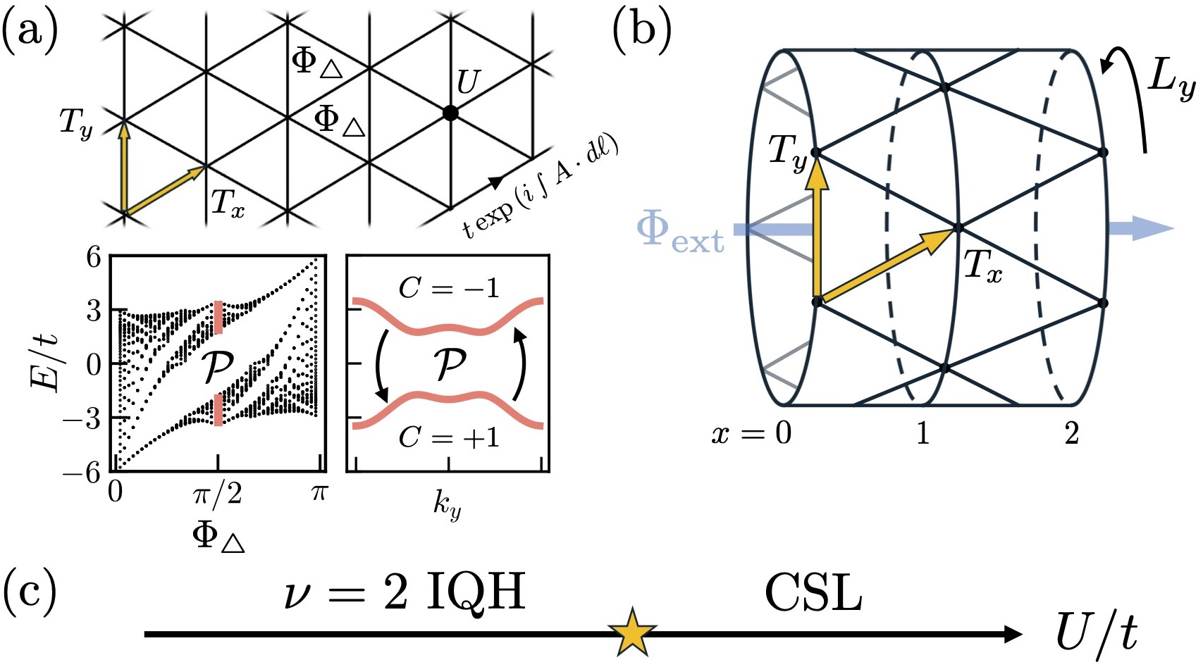
Figure 1: (a) Upper panel: The Hofstadter-Hubbard model on the 2D triangular lattice, with magnetic translations $T_{x,y}$, on-site Hubbard $U$ interaction, and flux per triangular plaquette $\Phi_{\triangle}$ indicated. Lower left panel: “Hofstadter butterfly” representation of spectrum of non-interacting model in the plane of single-particle energy $E$ and flux per plaquette $\Phi_{\triangle}$. $\Phi_{\triangle}=\pi/2$ is the unique flux for which the Hamiltonian enjoys a doubled “magnetic” unit cell and a particle-hole symmetry $\mathcal{P}$ relating opposite $C=\pm 1$ bands [lower right panel]. (b) A finite segment of the infinite-length, circumference-$L_{y}$ cylinder geometry, threaded by $\Phi_{\text{ext}}$ external magnetic flux. With the chosen “YC” cylindrical geometry, the translation $T_{y}$ is orthogonal to the cylinder axis and $x\in\mathbb{Z}$ indexes rings. (c) Expected 2+1D phase diagram at half-filling. As interactions increase, the spin-degenerate integer quantum Hall (IQH) ground state undergoes a quantum phase transition into a Kalmeyer-Laughlin chiral spin liquid (CSL). By studying both even and odd finite-circumference cylinders, we shed light on the existence and nature of this transition.

A model electronic system thought to host both conventional and CSL electronic phases is the triangular Hofstadter-Hubbard model (see Fig. 1a) in the regime of strong orbital magnetic flux, where the CSL may be favored energetically by both geometric frustration [15, 16] and the explicit breaking of time-reversal symmetry [17, 7]. The Hofstadter-Hubbard model is parametrized by an on-site interaction $U$ and a nearest neighbor hopping with Peierls phases corresponding to a flux of $\Phi_{\triangle}$ per elementary plaquette. When $\Phi_{\triangle}=\pi/2$ per triangle, this system realizes a spin-unpolarized integer quantum Hall (IQH) insulator at small values of the Hubbard interaction, with $\sigma_{xy}=2e^{2}/h$, obtained by filling the lower topological sub-band in both spin sectors. This state possesses a gap to spin and charge excitations, is topological and has a spin-degenerate charged edge mode. At very large $U$ and density of one electron per site, the state is a Mott insulator: the leading term in the $t/U$ expansion around the infinite-$U$ Mott limit shows that the low-energy physics is governed by the conventional antiferromagnetic nearest-neighbor $S=1/2$ Heisenberg model with $J_{H}\sim t^{2}/U$, which has $120^{\circ}$ antiferromagnetic order at $T=0$, so that the ground state is non-topological, with fully-gapped charge excitations and soft (Goldstone) spin excitations.

Carrying out the $t/U$ expansion to higher order suggests the existence of a CSL phase intermediate between the Mott/AF and IQH phases: the next correction is a third-order chiral term $S\cdot S\times S$ with coefficient $J_{\triangle}\sim t^{3}\sin\Phi_{\triangle}/U^{2}$. In the presence of the magnetic flux this term explicitly breaks both time-reversal and parity symmetry [17, 7]. Numerical studies of the $J_{H}$-$J_{\triangle}$ spin Hamiltonian have indeed revealed a CSL ground state for large enough $J_{\triangle}/J_{H}$ [18, 19], although at these values the accuracy of truncating the $t/U$ expansion at third order may be questioned. Very recently Kuhlenkamp et al. presented cylinder iDMRG evidence of an intermediate CSL phase for $U\gtrsim 10t$ at fluxes $\Phi_{\triangle}=\pi/3,\pi/2$ [11]. The CSL phase was identified by the absence of charge pumping as flux was threaded through the cylinder and the presence of appropriate degeneracies in the entanglement spectrum.

Supposing one accepts the existence of an intermediate CSL phase, the question of the nature of the IQH-CSL transition arises. A parton theory in which one decomposes the electron into a bosonic chargon $b$ carrying the charge and a fermionic spinon $f$ carrying the spin index, $c_{\sigma}=bf_{\sigma}$ has been proposed [14, 12]. This decomposition requires an emergent gauge field $a$, corresponding to the relative phase between the partons, under which they carry opposite unit $U(1)$ charge. In both the IQH and CSL phases the spinon occupies both $C=1$ magnetic sub-bands descending from the electronic bandstructure, while at the electronic IQH-CSL phase transition the chargon and the gauge field together undergo a superconductor-Mott phase transition [12]. The dynamical gauge field $a$ is responsible not only for producing the correct topological response on both sides of the transition, but also for gapping out the charge sector in the IQH phase through the Anderson-Higgs mechanism [20, 21], and allowing for spinon deconfinement in the CSL [22, 23, 24]. The parton representation and related slave-particle numerical studies on honeycomb and square lattices  [14, 25] have provided a physically intuitive, yet incomplete mean-field picture of the putative continuous transition. The iDMRG investigation of Ref. [11] revealed the IQH-CSL transition only as a crossover indicated by a weak maximum in a correlation length. Further investigation of the CSL phase and the IQH-CSL transition is therefore needed.

In this work we use a compactification to an infinite-length, finite-radius cylinder [see Fig. 1(b)] in combination with a symmetry analysis with large-scale iDMRG simulations [26, 27] on cylinders of circumference $L_{y}=3$ to $6$ to characterize the nature of the IQH and CSL states, as well as the transition between them. Our symmetry analysis is based on an operator that is a combination of particle-hole interchange and translation, which we show explicitly is spontaneously broken for interactions above a critical interaction strength for odd-circumference cylinders. We further show that the broken symmetry occurs together with the degeneracy pattern in the entanglement spectrum expected for a CSL phase. We present numerical evidence that this transition is in fact continuous and argue that in the limit of infinite cylinder radius, this transition evolves into a continuous 2+1D IQH-CSL quantum phase transition featuring critical fluctuations in the charge density and other spin rotationally-invariant observables.

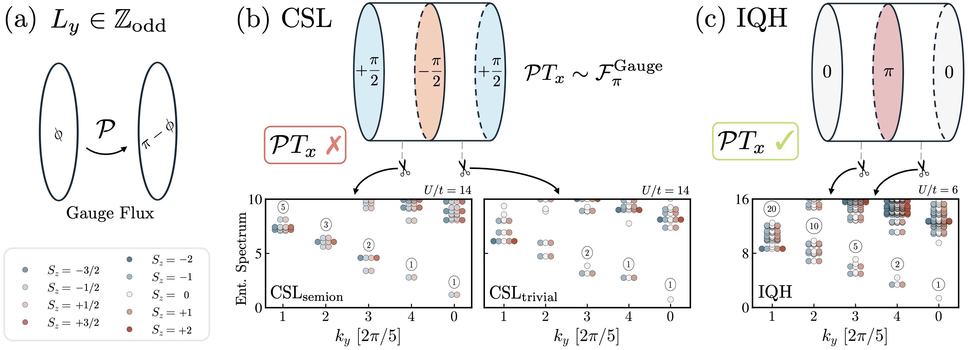
Figure 2: CSL symmetry-breaking at odd circumference. (a) Graphical illustration of the action of the particle-hole symmetry operator $\mathcal{P}$ which transforms the gauge flux through a ring of an odd-$L_{y}$ cylinder, from $\phi$ to $\pi-\phi$. (b) Upper panel: In an odd-$L_{y}$ CSL ground state, the alternating pattern $+\pi/2,-\pi/2,\dots$ of these gauge fluxes spontaneously breaks $\mathcal{P}T_{x}$ symmetry, whose action is equivalent to the threading of $\pi$ gauge flux. Lower panel: the low-lying entanglement eigenvalues at cuts between two pairs of rings, which not only exhibit the approximate degeneracy expected for the CSL at each $S_{z}$ [see circled numerals], but also transform as half-integer spin representations only at every other cut, signalling SSB of $\mathcal{P}T_{x}$. (c) In contrast, the internal gauge flux configuration [upper panel] and entanglement spectrum [lower panel] of the IQH state are consistent with it being a unique, symmetry-preserving ground state.

Model, symmetry operator and cylinder compactification—We study the Hofstadter-Hubbard model on the triangular lattice, defined pictorially in Fig. 1(a). In this model, electrons hop between nearest-neighboring sites and experience an Aharonov-Bohm phase of $\Phi_{\triangle}$ upon orbiting a triangular plaquette. Note that this model focuses on the consequences of the orbital motion, and sets the Zeeman coupling to zero. We fix $\Phi_{\triangle}=\pi/2$, which endows the Hamiltonian with a unitary particle-hole (PH) symmetry $\mathcal{P}$ acting as [28]

$$\mathcal{P}c^{\dagger}_{x,y}\mathcal{P}^{-1}=(-1)^{x+y}(i\sigma_{y})c_{x,y},\quad\mathcal{P}i\mathcal{P}^{-1}=+i,$$ (1)

on fermionic operators, where we have attached a conventional spin rotation $\sigma_{y}$ to the naive definition of particle-hole transformation in order for $\mathcal{P}$ to leave the spin operator $\bm{S}=\frac{1}{2}c^{\dagger}\bm{\sigma}c$ invariant (see SM for details [29]). The flux induces a magnetic translation algebra $T_{x}T_{y}=-T_{y}T_{x}$ that we represent in a gauge where

$$T_{x}c^{\dagger}_{x,y}T_{x}^{-1}=(-1)^{y}c^{\dagger}_{x+1,y},\quad T_{y}c^{\dagger}_{x,y}T_{y}^{-1}=c^{\dagger}_{x,y+1}.$$ (2)

The commuting translations $(T_{x})^{2},T_{y}$ define a larger “magnetic” unit cell, whose resulting two sub-bands are related by $\mathcal{P}$ and carry opposite Chern number $C=\pm 1$. We fix the filling to $n=1$ electron per lattice site, which in the absence of interactions corresponds to full filling of the lowest spin-degenerate magnetic sub-band.

We now present the dimensional reduction of the problem to a cylinder. The key results of our study rely on the different symmetry breaking patterns that occur for even and odd circumferences $L_{y}$, which stem from generic properties of magnetic fields (both external and internal) in the chosen geometry. To illustrate how this arises, let us first consider the closed “tin can”-shaped surface specified by a pair of adjacent rings at $x$ and $x+1$. This surface is the union of $2L_{y}$ triangles on the outside of the cylinder, as well as an $L_{y}$-sided polygonal surface at $x$ and another at $x+1$ whose edges are the rings. Since $\pi/2$ external flux penetrates each outer triangle, Gauss’s law requires that the external magnetic flux through the two adjacent rings differ by $\pi L_{y}$ [30, 31]. These ring fluxes are therefore uniform when $L_{y}$ is even, but are staggered when $L_{y}$ is odd, which explicitly breaks $T_{x}$ symmetry.

Let us momentarily focus on the odd case and fix the sequence of ring fluxes to alternate between $0$ and $\pi$. In this case, the system nonetheless respects a combined translation-like symmetry, namely the product of $\mathcal{P}$ and $T_{x}$—which we refer to as PH-glide—in spite of each being individually broken by the compactification. The IQH state, being adiabatically connected to the (unique) ground state of the non-interacting Hamiltonian, is invariant under PH-glide symmetry.

We argue, however, that the CSL phase must break $\mathcal{P}T_{x}$ spontaneously when $L_{y}$ is odd. To see this, note that the CSL is a Mott insulating phase. Thus, we may consider the limit where charge fluctuations are frozen out, e.g. by increasing $U\to\infty$ while holding the three-spin chiral term at a fixed favorable strength. Since the particle-hole operation is transparent to the spin operator, $\mathcal{P}\bm{S}\mathcal{P}^{-1}=\bm{S}$, this results in a spin model with a pure translation symmetry $t_{x}$. Since each ring contains an odd number of spin-$1/2$ moments, the Lieb-Schulz-Mattis theorem requires that any gapped ground state be at least two-fold degenerate [33], e.g., by spontaneously breaking $t_{x}$. One way to understand the translation symmetry breaking of the CSL, in particular, is by leveraging its anyonic content. Namely, the properties of the CSL under translations are captured by viewing it has hosting a spinon in each unit cell of the triangular lattice [34, 35, 36]. Because these spinons have semionic statistics, the action of $t_{x}$ translation—which moves $L_{y}$ many spinons across any given cut—necessarily permutes the two minimally-entangled CSL ground states [37] when $L_{y}$ is odd [38, 39]. In other words, the only $t_{x}$-symmetric ground states are long-range-entangled CSL “cat” states, implying that translation is spontaneously broken [40].

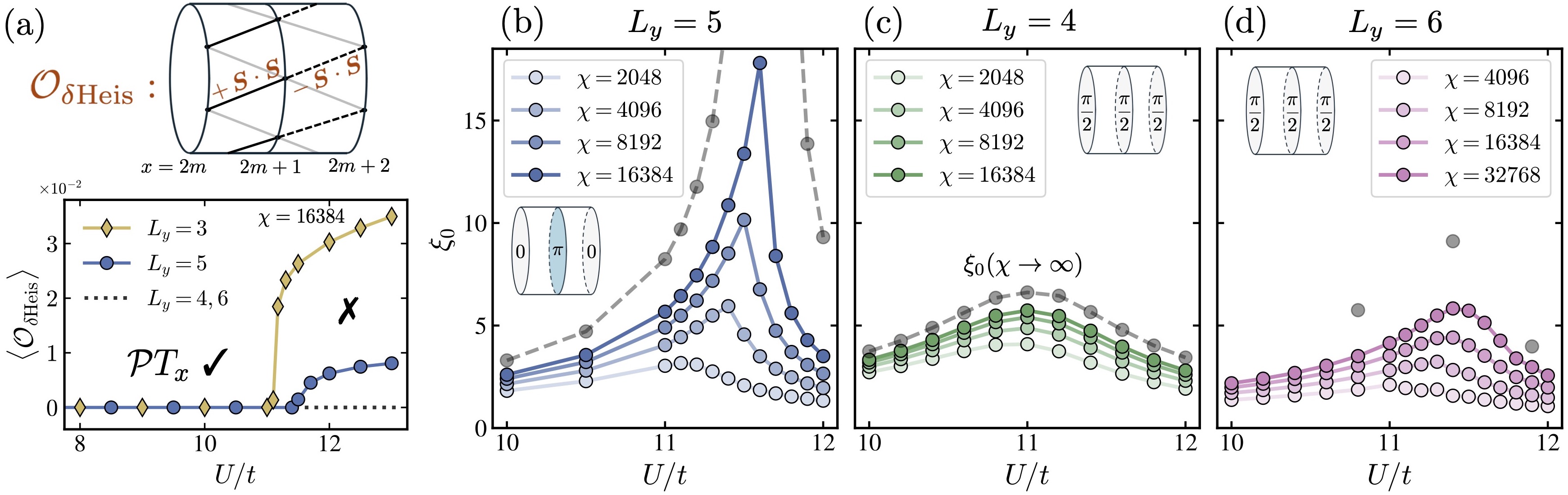
Figure 3: Evidence for the IQH-CSL phase transition. (a) Upper panel: Sketch of three rings of cylinder at indicated $x$ values, with solid and dashed lines showing along which staggered-Heisenberg order parameter $\mathcal{O}_{\delta\mathrm{Heis}}$ [defined in Eq. (3)] changes under glide particle-hole symmetry $\mathcal{P}T_{x}$ on odd-circumference cylinders. Lower panel: Magnitude of the staggered Heisenberg order parameter plotted against $U/t$ for cylinder widths indicated and with $\mathcal{P}T_{x}$ preserving and broken phases indicated by the check and cross symbols. Consistent with the recovery of this symmetry at the putative 2+1D critical point, the magnitude of the order parameter [bottom left] decreases substantially from $L_{y}=3$ to $5$. (b-d) Correlation length in the $(Q,S_{z},k_{y})=\bm{0}$ charge sector, plotted against interaction strength, for a range of MPS bond dimensions [increasing light to dark] and extrapolated to infinite bond dimension [gray points]; the insets specify the external flux threading each of the cylinder rings. (b) At circumference $L_{y}=5$, the $\mathcal{P}T_{x}$ symmetry-breaking is associated with a diverging correlation length. (c) While both the IQH and CSL states are fully-symmetric on even-$L_{y}$ cylinders, the dominant correlation length is consistently charge-neutral, peaking strongly for $\Phi_{\text{ext}}=\pi/2$ external flux threading the cylinder (see inset). The maximum extrapolated value of the correlation length increases from $L_{y}=4$ to $6$, consistent with an approach to a continuous transition in the thermodynamic limit.

It is illustrative to phrase the above discussion in terms of operations on the internal gauge field introduced in the parton construction. For simplicity, let us focus on saddle point configurations of the gauge field on each side of the transition, ignoring fluctuations. In both the CSL and IQH ground states, the gauge flux through the triangular surface plaquettes should match the external flux, $\phi_{\triangle}=\pi/2$ [6, 7, 12]. Thus, the only remaining gauge-invariant degree of freedom is the gauge flux through the cylinder rings; assuming $T_{x}^{2}$ is unbroken and $L_{y}$ is odd, we may parameterize the two fluxes as $(\phi,\phi+\pi)$, differing by $\pi$ due to Gauss’s law, as invoked above. Since the minimally-entangled CSL ground states are adiabatically connected to the Mott limit in which $\mathcal{P}$ acts trivially, their ring flux patterns are restricted to be $(\pi/2,-\pi/2)$ and $(-\pi/2,\pi/2)$, which are insensitive to the action of $\mathcal{P}$ on ring fluxes, namely $\phi\to\pi-\phi$ (Fig. 2a). We readily see that these two configurations are related by $\mathcal{P}T_{x}$, exposing the two-fold degeneracy and SSB of the CSL (Fig. 2b, top) [41]. In the IQH phase, on the other hand, the Meissner effect pins together the internal and external gauge fields [42]. The resulting flux pattern $(0,\pi)$ maps into itself under $\mathcal{P}T_{x}$, consistent with a unique, gapped ground state (Fig. 2c, top).

While the small $U$ IQH phase does not break the glide-PH symmetry and the intermediate $U$ CSL phase has a two-fold symmetry breaking pattern on odd circumference cylinders, the large $U$ $120^{\circ}$ phase breaks translational symmetry (including the glide PH) in a threefold spatial pattern.

Numerical observation of phase transition—We first comment on evidence for the phases themselves. The primary diagnostic of chiral topological behavior is the behavior of the charge-resolved entanglement spectrum (ES) [43, 44] at a bipartition of the system into two semi-infinite halves, in this case between any pair of adjacent rings [40, 11]. We exploit the relationship between the physical and entanglement edges [45, 43, 46], namely that the low-lying states in the entanglement spectrum correspond to those of the edge CFT [47, 48, 49, 50].

Within the bulk-boundary correspondence, the CSL is expected to host gapless edges described at low energies by a free bosonic conformal field theory [51]. The counting of low-energy states as a function of momentum in each conserved charge sector can be obtained combinatorially: for fixed $n\in\mathbb{Z}_{\geq 0}$ and associated momentum $q_{y}=2\pi n/L_{y}$, one considers a linearly dispersing mode and imagines exciting states from below to above the Fermi level. Note that these bosonic objects are charge and spin-neutral but carry momentum. The counting sequence is namely the number of integer partitions of $n$: $(1,1,2,3,5,\dots).$ On the other hand, the IQH phase has two independent bosonic edge modes. Here, the total momentum must be the sum of those of the two flavors. Working out the “two-color” integer partitions of $n$ yields the counting $(1,2,5,10,20\dots).$ These expectations are borne out in our numerics; see Fig. 2(b,c).

We now investigate the transition. Consistent with the expectations above, we confirm that the CSL phase spontaneously breaks $\mathcal{P}T_{x}$ symmetry on odd-$L_{y}$ cylinders. We first find that the bipartite ES in the CSL phase exhibits a two-ring periodicity, which implies SSB. In contrast, the ES of the IQH is fully invariant under the action of $\mathcal{P}T_{x}$, as shown in Fig. 2(c). Second, by scanning $U/t$ and inspecting the transfer matrix spectrum, we identify a diverging correlation length for the accessible odd-circumference cylinder geometries, namely $L_{y}=3,5$. The divergence is found to belong to the $(Q,S_{z},k_{y})=\bm{0}$ charge sector (see Fig. 3b for the $L_{y}=5$ and the SM [29] for $L_{y}=3$). The spontaneous breaking of glide-PH symmetry is the source of this quasi-(1+1)D criticality. To substantiate this, we identified an order parameter $\mathcal{O}_{\delta\mathrm{Heis}}=\sum_{m}\mathcal{O}^{\delta\mathrm{Heis}}_{2m}$, where

$$\mathcal{O}^{\delta\text{Heis}}_{x}=L_{y}^{-1}\sum_{y}\bm{S}_{x,y}\cdot\bm{S}_{x+1,y}-\bm{S}_{x+1,y}\cdot\bm{S}_{x+2,y}.$$ (3)

The operator $\mathcal{O}_{\delta\mathrm{Heis}}$ is both charged under $\mathcal{P}T_{x}$ and condenses in the CSL phase [see Fig. 3(a)], signaling SSB. We remark that threading external flux $\Phi_{\text{ext}}=\pi/2$ through an odd-circumference cylinder reduces the transition to a crossover, owing to the fact that flux threading explicitly breaks glide-PH symmetry unless $\Phi_{\text{ext}}\in\pi\mathbb{Z}$ (see SM [29]).

On the even-circumference geometries $L_{y}=4$ and $6$, we reproduce the weak crossover, with a correlation length of $\sim 2$ lattice sites, found by Kuhlenkamp et al. for $L_{y}=6$ and $\Phi_{\text{ext}}=0$ [11]. This is consistent with the absence of translation symmetry-breaking in the even-circumference Mott limit. Upon threading $\Phi_{\text{ext}}=\pi/2$ external flux through each of these systems, we observe dramatically larger values of the correlation length for $U$ near $U_{c}$ (Fig. 3), notably in the same neutral sector in which the odd-circumference correlation length diverges [see Fig. 3(c,d)]. We also perform an extrapolation to infinite bond dimension following Ref. [52]; see SM for details [29]. The maximal extrapolated value is $\xi=6.6$ at $L_{y}=4$, increasing substantially to $\xi=9.1$ at $L_{y}=6$. Consistent with the view that accurate estimation of the 2+1D gap and other properties requires consideration of all threaded cylinder fluxes [53], we conjecture that the $\Phi_{\text{ext}}=\pi/2$ threaded system is more reflective of the thermodynamic limit than the unthreaded system, and that larger even-$L_{y}$ geometries will exhibit an increasingly-sharp sequence of crossovers toward 2+1D critical behavior in the charge-neutral sector.

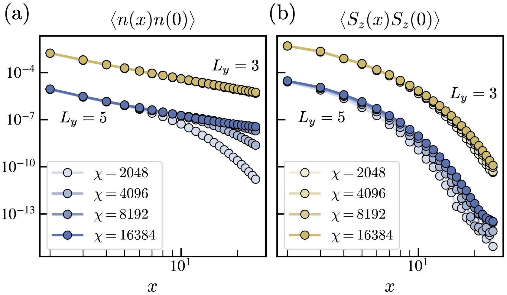
Figure 4: Density-density [left panel] and spin-spin [right panel] connected correlations for odd-circumference cylinders with $U$ tuned to the respective critical points, $U_{*}(L_{y}=3)=11.1$ and $U_{*}(L_{y}=5)=11.6$. Both $L_{y}=5$ correlation functions are scaled down by 100 for ease of viewing. (a) Density-density correlations decay nearly algebraically at the IQH-CSL transition, pointing to the presence of gapless charge-neutral excitations in the 2+1D limit. (b) In contrast, correlations of the spin density decay exponentially with no apparent enhancement from $L_{y}=3$ to $5$, suggesting that the excitations are spin-rotationally-invariant singlets.

Remarkably, the critical fluctuations at the odd-$L_{y}$ critical points manifest not only in the order parameter, but also in the charge density. This is seen manifestly in the connected density-density correlations $\langle n(x)n(0)\rangle$, with $n(x)$ averaged over the ring $x$, which we find to decay approximately algebraically, i.e., linearly on a log-log scale [see Fig. 4(a)] However, estimation of the 2+1D critical exponents from these data is hampered by the fact that the critical features of the thermodynamic limit need only show up in the regime $1\ll x\ll L_{y}$, which is inaccessible for the presently-tractable system sizes. While PH-glide is no longer broken for $L_{y}=4,6$ and the operator Eq. (3) no longer condenses (see Fig. 3a), we also observe that their enhanced correlation length is accompanied by an apparent algebraic plateau in $\langle n(x)n(0)\rangle$ over the scale of the correlation length (see SM [29]).

Curiously, we do not observe critical behavior in the odd-$L_{y}$ connected correlations of the spin density $S_{z}$ [Fig. 4(b)], which is also neutral under the conserved charge and spin $U(1)$ symmetries. However, since $S_{z}$ may be rotated into $S_{x}$ by a global spin rotation, under which the CSL is invariant, this is consistent with our not observing a diverging correlation length in the $(Q,S_{z})=(0,\hbar)$ sector of the transfer matrix. Altogether, under the assumption that this behavior persists for the entire sequence of odd circumferences, our observations suggest that the 2+1D critical point hosts gapless, charge-neutral spin-singlet excitations.

We remark that these data are consistent with the partonic view that the transition into the IQH corresponds to chargon condensation. While the chargon is not gauge invariant and may not develop conventional long-range connected correlations, at the critical point the combination of the chargon, anti-chargon and gauge string is a gapless neutral excitation [42]. Interestingly, the power law correlations presented in Fig. 4 show that the physical charge density operator, which has nonzero overlap with the gauge-invariant chargon density $b^{\dagger}(x)b(x)$, produces a state with a nonzero overlap with the critical excitations when applied to the ground state, raising the intriguing possibility that the critical fluctuations can be experimentally observed.

Discussion—By combining numerical data on both even and odd-circumference cylinder geometries, we have provided evidence that the CSL-IQH transition is in fact continuous in the Hofstadter-Hubbard model at $\pi/2$ flux per triangle and that critical properties are already manifest at the numerically-accessible circumferences $3\leq L_{y}\leq 6$. Our finding that critical fluctuations appear in the charge density correlation function, which may be probed by experimental or numerical measurement of the structure factor, raise the possibility of experimental and numerical investigation of this transition.

This paradigmatic Hofstadter-Hubbard system provides a uniquely minimal and experimentally-relevant setting [10, 11] in which to study a fundamental phase transition at the interface of spin liquid and quantum Hall physics. As such, a more complete understanding of this transition is an important task for future work. Quantitatively, our investigation clarifies the possible observable, numerical signatures that may be used to probe the phase transition in a variety of numerical methods, such as AFQMC, VMC, or fermionic PEPS, which may be able to access larger system sizes or spectral signatures of spin-charge separation [54, 55, 56].

An important broader message of this work is that the ability to extrapolate 2+1D physics from dimensionally-reduced numerical data—namely on infinite cylinder geometries—is greatly enhanced by carefully considering the manner in which candidate ground states and their phase transitions respond to dimensional reduction and to external fields that become boundary effects in the thermodynamic limit. Applying such techniques more systematically, it would be valuable to characterize the contexts in which UV features of Mott phases, namely spin liquids, may be leveraged to better characterize their charge fluctuation-induced phase transitions.

Acknowledgements—We acknowledge useful discussions with E. Altman, S. Chatterjee, O. Gauthé, M. Knap, C. Kuhlenkamp, J.Y. Lee, C. Liu, F. Pollmann, Z. Weinstein, and especially X.Y. Song. The Flatiron Institute is a division of the Simons Foundation. AJM was supported in part by Programmable Quantum Materials, an Energy Frontier Research Center funded by the U.S. Department of Energy (DOE), Office of Science, Basic Energy Sciences (BES), under award DE-SC0019443. S.D. acknowledges support from the NSERC PGSD fellowship. M.Z. and S.D. were supported by the U.S. Department of Energy, Office of Science, National Quantum Information Science Research Centers, Quantum Systems Accelerator (QSA). This research is funded in part by the Gordon and Betty Moore Foundation’s EPiQS Initiative, Grant GBMF8683 to T.S. Calculations were performed using the TeNPy Library [57].

oneΔ

Supplementary Material: “Chiral Spin Liquid and Quantum Phase Transition in the Triangular Lattice Hofstadter-Hubbard Model”

Appendix A Hamiltonian construction at all rational fluxes

For the underlying triangular lattice — with the “YC” orientation on the cylinder (where the $\hat{y}$ site-to-site distance is the NN distance $a$) — we take the following Bravais vectors:

$$\bm{a}_{1}=a\left(\frac{\sqrt{3}}{2}\hat{x}+\frac{1}{2}\hat{y}\right),\qquad\bm{a}_{2}=a\hat{y}\qquad\text{(YC)},$$ (1)

whose corresponding reciprocal lattice vectors are

$$\bm{b}_{1}=\frac{4\pi}{\sqrt{3}a}\hat{x},\qquad\bm{b}_{2}=\frac{2\pi}{a}\left(-\frac{\hat{x}}{\sqrt{3}}+\hat{y}\right)\qquad\text{(YC)}.$$ (2)

SI Choosing the magnetic unit cell

The following discussion applies to both the YC and XC lattice geometries. Let the flux per parallelogram be

$$\Phi=\frac{p}{q}\Phi_{0},$$ (3)

where $\Phi_{0}=\frac{2\pi\hbar}{e}\sim 2\pi$ in units where $\hbar/e=1.$ The above definition of flux is convenient for defining the geometry, but we briefly remark that the flux $\Phi/2$ per triangle — which is the smallest traversable plaquette — is the quantity with respect to which physical behavior (e.g., the Hofstadter spectrum) must be $\Phi_{0}$-periodic. In any case, the corresponding magnetic field strength is

$$B=\frac{\Phi}{A_{\text{par}}}=\frac{p\Phi_{0}/q}{\frac{\sqrt{3}}{2}a^{2}}=\frac{2p\Phi_{0}}{\sqrt{3}q}a^{-2}.$$ (4)

Regardless of the parity of $q$, there will be $q$ magnetic sublattice sites in the magnetic unit cell, which we label by $\tau=0,\dots,q-1.$ When $q$ is even, the magnetic Bravais vectors are

$$\bm{R}_{1}=q\bm{a}_{1}-\frac{q}{2}\bm{a}_{2}\propto\hat{x},\qquad\bm{R}_{2}=\bm{a}_{2}\propto\hat{y},\qquad(q\ \text{even}),$$ (5)

whose total area $A_{\text{muc}}$ (for either YC or XC) is precisely that of $2q$ triangles of area $\frac{\sqrt{3}}{4}a^{2}.$ The associated reciprocal lattice vectors are

$$\bm{G}_{1}=\frac{1}{q}\bm{b}_{1}\propto\hat{x},\qquad\bm{G}_{2}=\frac{1}{2}\bm{b}_{1}+\bm{b}_{2}\propto\hat{y},\qquad(q\ \text{even}).$$ (6)

As a sanity check, the total of the magnetic Brillouin zone (mBZ) is then

$$A_{\text{mBZ}}=|\bm{G}_{1}\times\bm{G}_{2}|=(2\pi)^{2}\frac{2}{q\sqrt{3}a^{2}}=\frac{(2\pi)^{2}}{A_{\text{muc}}}.$$ (7)

When $q$ is odd, the enclosing magnetic unit cell again contains exactly $2q$ triangles, but we take

$$\bm{R}_{1}=q\bm{a}_{1}-\frac{q-1}{2}\bm{a}_{2},\qquad\bm{R}_{2}=\bm{a}_{2}\propto\hat{y},,\qquad(q\ \text{odd}),$$ (8)

whose total area is once again

$$|\bm{R}_{1}\times\bm{R}_{2}|=q|\bm{a}_{1}\times\bm{a}_{2}|=\frac{q\sqrt{3}}{2}a^{2}=A_{\text{muc}}.$$ (9)

The reciprocal lattice vectors are now

$$\bm{G}_{1}=\frac{1}{q}\bm{b}_{1},\qquad\bm{G}_{2}=\frac{q-1}{2q}\bm{b}_{1}+\bm{b}_{2},\qquad(q\ \text{odd}),$$ (10)

which also satisfy the inverse area relationship, Eq. (7).

In Fig. LABEL:fig:YC_c2zsymm_locations, we illustrate the choice of magnetic unit cell for both odd and even $q$ for the YC triangular lattice boundary conditions. For both even and odd denominator $q,$ note that the enclosing magnetic unit cell contains exactly $2q$ triangles, so $2\pi p\in 2\pi\mathbb{Z}$ total flux. In addition, we position the sublattice sites $\tau$ within the magnetic unit cell in such a way that all the sites within magnetic unit cell $\bm{R}$ transform under $C_{2z}$ into sites in $-\bm{R}$. In particular, the sites in the home magnetic unit cell transform into one another in a clean way. We achieved this by further partitioning the odd-$q$ geometries into two subclasses. In Fig. LABEL:fig:XC_c2zsymm_locations, we make the same specifications for the XC boundary conditions.

SII Hamiltonian and choice of vector potential

Placing the underlying triangular lattice on the cylinder, let the resulting system have circumference $L_{y}$, i.e., the points $\bm{r}\sim\bm{r}+L_{y}\bm{a}_{2}$ are geometrically identified. Let the lattice sites be indexed by

$$\bm{r}=x\bm{a}_{1}+y\bm{a}_{2},$$ (11)

which defines our coordinate system, where $(x,y)\in\mathbb{Z}^{2}.$ Since $\bm{a}_{2}$ is purely vertical in both geometries, then $x$ indexes the rings, and $y$ is a integer spatial index within each ring. To generate complex hoppings and modify the translation algebra to a magnetic translation algebra, we introduce an external $U(1)$ vector potential. We assume that it is linear and that its curl is the magnetic field:

$$\bm{A}(\bm{r})=M\bm{r},\qquad\nabla\times\bm{A}(\bm{r})=B\hat{z},$$ (12)

where $B$ is as in Eq. (4). The hoppings are obtained from the vector potential via the Peierl’s substitution, for which we adopt the following sign convention:

$$t_{\bm{r}^{\prime}\leftarrow\bm{r}}=t\exp\left(i\int^{\bm{r}^{\prime}}_{\bm{r}}\bm{A}(\bm{\ell})\cdot d\bm{\ell}\right)=t\exp\left(i\bm{A}\left(\frac{\bm{r}^{\prime}+\bm{r}}{2}\right)\cdot(\bm{r}^{\prime}-\bm{r})\right),$$ (13)

where the second equality is due to linearity of $\bm{A}(\bm{r})$. Our convention is that the single-particle Hamiltonian is (note the minus sign):

$$\hat{h}=-\sum_{\bm{r}^{\prime},\bm{r}}c^{\dagger}(\bm{r}^{\prime})t_{\bm{r}^{\prime}\leftarrow\bm{r}}c(\bm{r}),$$ (14)

where we only include nearest-neighbour hopping on the triangular lattice, for which

$$t_{\bm{r}^{\prime}\leftarrow\bm{r}}=te^{i\bm{A}\left(\frac{\bm{r}^{\prime}+\bm{r}}{2}\right)\cdot(\bm{r}^{\prime}-\bm{r})}.$$ (15)

To constrain the form Eq. (12), we remark that the terms $x\hat{x}$ and $y\hat{y}$ are curl-free, whereas $Bx\hat{y}$ and $-By\hat{x}$ — the standard Landau gauges on the rectangular lattice — have the correct curl. We therefore reason that the most general permissible $M$ is given by

$$M=B\begin{pmatrix}\alpha&\gamma-1\\ \gamma&\beta\end{pmatrix},$$ (16)

where $\alpha,\beta,\gamma\in\mathbb{R}$. We will now demand that the choice of vector potential is compatible with our chosen geometry of magnetic Bravais vectors. Specifically, we ask that the Peierl’s hoppings generated by $\bm{A}$ are periodic in the chosen Bravais vectors. This allows us to place the system easily on a torus or cylinder, provided the system tiles an integer number of magnetic unit cells. Quantitatively, we demand that the RHS of Eq. (13) is invariant under shifts of the argument of $\bm{A}$ by the magnetic Bravais vectors $\bm{R}_{1}$ and $\bm{R}_{2}$, for all bond vectors $\bm{r}^{\prime}-\bm{r}$. By linearity of the vector potential, and since the bond vectors are linear combinations of $\bm{a}_{1}$ and $\bm{a}_{2}$, it suffices to require that

$$\bm{a}_{i}\cdot\bm{A}(\bm{R}_{j})\in 2\pi\mathbb{Z},$$ (17)

for all $i,j$. Following Ref. [58], an elegant solution can be found in terms of the reciprocal vectors of the underlying triangular lattice. We take the following since $\bm{b}_{1}\propto\hat{x}$ for both YC and XC geometries, and we want the vector potential to be independent of $y$:

$$\bm{A}(\bm{r})=\frac{\Phi}{(2\pi)^{2}}(\bm{r}\cdot\bm{b}_{1})\bm{b}_{2}.$$ (18)

where $\Phi$ is the flux per parallelogram. Noting the vector identity

$$\left[\nabla\times\left((\bm{r}\cdot\bm{Q})\bm{P}\right)\right]_{i} =\epsilon_{ijk}\partial_{j}\left(\bm{r}_{\ell}\bm{Q}_{\ell}\bm{P}_{k}\right)=\epsilon_{ijk}\bm{Q}_{j}\bm{P}_{k}=(\bm{Q}\times\bm{P})_{i},$$ (19)

then

$$\bm{B}(\bm{r}) =\nabla\times\bm{A}(\bm{r})=\frac{\Phi}{(2\pi)^{2}}\bm{b}_{1}\times\bm{b}_{2}=\frac{\Phi}{(2\pi)^{2}}\frac{(2\pi)^{2}}{A_{\text{par}}}\hat{z}=\frac{\Phi}{A_{\text{par}}}\hat{z}.$$ (20)

Moreover, it can be shown to have the required periodicity property:

$$\bm{a}_{i}\cdot\bm{A}(\bm{R}_{j}) =\frac{\Phi}{(2\pi)^{2}}(\bm{R}_{j}\cdot\bm{b}_{1})\bm{b}_{2}\cdot\bm{a}_{i}=\delta_{i,2}\frac{2\pi p/q}{2\pi}(\bm{R}_{j}\cdot\bm{b}_{1})=\delta_{i,2}\frac{p}{q}\bm{R}_{j}\cdot\bm{b}_{1},$$ (21)

which clearly vanishes when $j=2.$ Otherwise,

$$\bm{a}_{i}\cdot\bm{A}(\bm{R}_{1}) =\delta_{i,2}\frac{p}{q}\left(\begin{cases}\left(q\bm{a}_{1}-\frac{q}{2}\bm{a}_{2}\right)\cdot\bm{b}_{1}&q\text{ even}\\ \left(q\bm{a}_{1}-\frac{q-1}{2}\bm{a}_{2}\right)\cdot\bm{b}_{1}&q\text{ odd}\end{cases}\right)=2\pi p\delta_{i,2},$$ (22)

so that, indeed, in either case:

$$\bm{a}_{i}\cdot\bm{A}(\bm{R}_{j})\in 2\pi\mathbb{Z}.$$ (23)

Appendix B Threading flux

SI Affine-linear vector potential implementation

When dimensionally-reducing the lattice system to the cylinder, the charge and spin flux through the cross sections of the cylinder distinguish gauge-inequivalent systems. This additional flux can be implemented by adding a constant term to the vector potential:

$$\bm{A}(\bm{r})\longrightarrow\bm{A}_{\phi}(\bm{r})=\bm{A}(\bm{r})+\phi\frac{\bm{b}_{2}}{2\pi L_{y}},$$ (24)

where

$$\phi=\phi_{q}+\frac{\sigma_{z}}{2}\phi_{s}.$$ (25)

This modifies the hopping elements by

$$t_{\bm{r}+\bm{\delta}\leftarrow\bm{r}}\longrightarrow t_{\bm{r}+\bm{\delta}\leftarrow\bm{r}}^{\phi}=t_{\bm{r}+\bm{\delta}\leftarrow\bm{r}}\exp\left(i\frac{\phi}{2\pi}\frac{\bm{b}_{2}\cdot\bm{\delta}}{L_{y}}\right).$$ (26)

Since we made the choice $\bm{A}\propto\bm{b}_{2}$ for the original vector potential (in the absence of flux threading), then this is equivalent to a shift in the origin:

$$\bm{A}_{\phi}(\bm{r})=\bm{A}(\bm{r}+\bm{X}_{\phi})=\bm{A}(\bm{r})+\frac{\Phi}{(2\pi)^{2}}(\bm{X}_{\phi}\cdot\bm{b}_{1})\bm{b}_{2},$$ (27)

where

$$\bm{X}_{\phi}=\frac{\phi\bm{a}_{1}}{\Phi L_{y}}.$$ (28)

SII Twisted boundary condition implementation

For the purposes of numerical implementation, particularly in hybrid space where we exchange $y$ for $k_{y}$, it is convenient to instead implement flux threading via a twist in the boundary conditions. Starting with periodic boundary conditions $c^{\dagger}(\bm{r}+L_{y}\bm{a}_{2})=c^{\dagger}(\bm{r})$ for $\phi=0$, define a new set of operators

$$c^{\dagger}_{\phi}(\bm{r})=c^{\dagger}(\bm{r})\exp(iy\phi/L_{y})=c^{\dagger}(\bm{r})\exp\left(i\phi\frac{\bm{b}_{2}\cdot\bm{r}}{2\pi L_{y}}\right).$$ (29)

Then instead of implementing Eq. (24), we can instead replace every instance of $c$ with $c_{\phi}$. This does not affect terms that depend solely on charge and spin densities, e.g., the Hubbard interaction. However, it will modify the hoppings in a way that is equivalent to Eq. (24). Under the operator replacement, the hoppings are replaced by

$$c^{\dagger}(\bm{r}+\bm{\delta})t_{\bm{r}+\bm{\delta}\leftarrow\bm{r}}c(\bm{r}) \longrightarrow c_{\phi}^{\dagger}(\bm{r}+\bm{\delta})t_{\bm{r}+\bm{\delta}\leftarrow\bm{r}}c_{\phi}(\bm{r})$$ (30)

$$=c^{\dagger}(\bm{r}+\bm{\delta})\exp\left(i\phi\frac{\bm{b}_{2}\cdot(\bm{r}+\bm{\delta})}{2\pi L_{y}}\right)t_{\bm{r}+\bm{\delta}\leftarrow\bm{r}}\exp\left(-i\phi\frac{\bm{b}_{2}\cdot\bm{r}}{2\pi L_{y}}\right)c(\bm{r})$$ (31)

$$=c^{\dagger}(\bm{r}+\bm{\delta})\exp\left(i\frac{\phi}{2\pi}\frac{\bm{b}_{2}\cdot\bm{\delta}}{L_{y}}\right)t_{\bm{r}+\bm{\delta}\leftarrow\bm{r}}c(\bm{r}),$$ (32)

which is exactly equivalent to Eq. (26). To see that Eq. (29) corresponds to a twisting of the boundary condition on the fermion operators, we note that

$$c^{\dagger}_{\phi}(\bm{r}+L_{y}\bm{a}_{2})=c^{\dagger}(\bm{r}+L_{y}\bm{a}_{2})\exp\left(i\phi\frac{\bm{b}_{2}\cdot(\bm{r}+L_{y}\bm{a}_{2})}{2\pi L_{y}}\right)=c_{\phi}^{\dagger}(\bm{r})\exp(i\phi).$$ (33)

The utility of this alternative formulation is that it leads to a clean numerical implementation upon fourier transforming $y\to k_{y}$. In particular, recall that $(x,y)=(\bm{r}\cdot\bm{b}_{1}/2\pi,\bm{r}\cdot\bm{b}_{2}/2\pi)$ and define

$$c_{\phi}^{\dagger}(x,k_{y})=\frac{1}{\sqrt{L_{y}}}\sum_{y}e^{-ik_{y}y}c_{\phi}^{\dagger}(x,y)\iff c_{\phi}^{\dagger}(x,y)=\frac{1}{\sqrt{L_{y}}}\sum_{k_{y}}e^{ik_{y}y}c_{\phi}^{\dagger}(x,k_{y}).$$ (34)

Note that this is the Fourier convention of TeNPy. When we express the Hamiltonian in the hybrid $xk_{y}$ representation, we find that all that’s required is to shift the allowed values of $k_{y}.$ To see this, we impose the twisted boundary condition Eq. (33) on the Fourier-expanded operators:

$$\frac{1}{\sqrt{L_{y}}}\sum_{k_{y}}e^{ik_{y}(y+L_{y})}c_{\theta}^{\dagger}(x,k_{y})=\frac{1}{\sqrt{L_{y}}}\sum_{k_{y}}e^{ik_{y}y}c_{\theta}^{\dagger}(x,k_{y})e^{i\phi},$$ (35)

so that

$$e^{ik_{y}L_{y}}=e^{i\phi}.$$ (36)

The allowed values of momenta are therefore quantized to:

$$k_{y}=\frac{2\pi}{L_{y}}\left(n+\frac{\phi_{q}}{2\pi}+\frac{\sigma_{z}\phi_{s}}{4\pi}\right),\qquad n\in\mathbb{Z},$$ (37)

which are shifted relative to the $\phi=0$ case. When the original Hamiltonian $\hat{H}_{\phi=0}$ is written in hybrid space, some coefficients will depend on $k.$ The only affect of the replacement Eq. (29) is then for those coefficients to instead be evaluated on these shifted set of allowed values.

Appendix C Two-band hopping Hamiltonian

SI Hamiltonian at $(p,q)=(1,2)$

Now let us specialize to the case $(p,q)=(1,2)$, which corresponds to $\Phi_{\triangle}=\pi/2$. To specify the unit cells (which each contain two sites), we often write $x=\tau+2u$, where $u\in\mathbb{Z}$, while $\tau\in\{0,1\}$ specifies the even/odd rings. With periodic boundary conditions and before flux insertion, the hoppings Eq. (15) take the particular form

$$t_{(x,y+1)\leftarrow(x,y)} =t\exp\left(i\bm{A}\left(x\bm{a}_{1}+y\bm{a}_{2}+\frac{\bm{a}_{2}}{2}\right)\cdot\bm{a}_{2}\right)$$

$$=t\exp\left(\frac{i}{4\pi}\left(x\bm{a}_{1}+y\bm{a}_{2}+\frac{\bm{a}_{2}}{2}\right)\cdot\bm{b}_{1}\bm{b}_{2}\cdot\bm{a}_{2}\right)$$

$$=t\exp\left(i\pi x\right),$$ (38)

$$t_{(x+1,y)\leftarrow(x,y)} =t\exp\left(i\bm{A}\left(\frac{\bm{a}_{1}}{2}+x\bm{a}_{1}+y\bm{a}_{2}\right)\cdot\bm{a}_{1}\right)$$

$$=t,$$ (39)

$$t_{(x+1,y-1)\leftarrow(x,y)} =t\exp\left(i\bm{A}\left(\frac{\bm{a}_{1}-\bm{a}_{2}}{2}+x\bm{a}_{1}+y\bm{a}_{2}\right)\cdot(\bm{a}_{1}-\bm{a}_{2})\right)$$

$$=t\exp\left(-i\bm{A}\left(\frac{\bm{a}_{1}-\bm{a}_{2}}{2}+x\bm{a}_{1}+y\bm{a}_{2}\right)\cdot\bm{a}_{2}\right)$$

$$=t\exp\left(-i\pi(x+1/2)\right).$$ (40)

We depict the resulting hopping phases in Fig. S1(a) for the lattice orientation where $\bm{a}_{2}=a\hat{y}$ is a nearest-neighbour bond; this becomes becomes the YC geometry when the system is placed on a cylinder under the identification $\bm{r}\sim\bm{r}+L_{y}\bm{a}_{2}$.

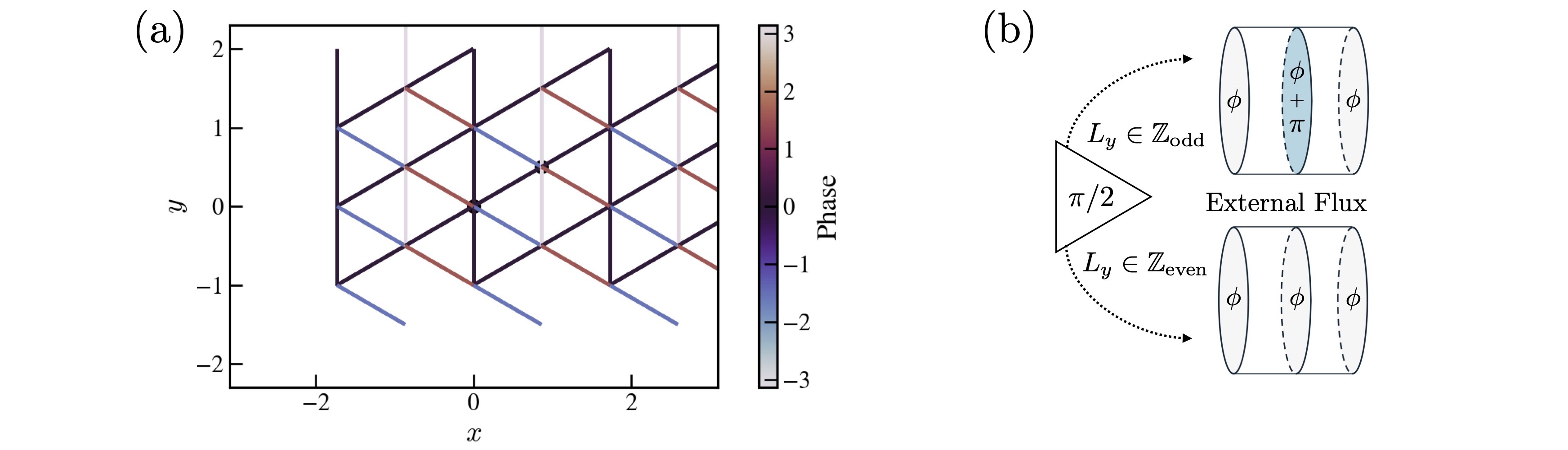
Figure S1: (a) Hopping phases for the $(p,q)=(1,2)$ two-band Hamiltonian corresponding to $\pi/2$ flux per triangle. The two black circles indicate the two sites in the magnetic unit cell. The phases indicated by the color bar are accrued when hopping upward, right-upward, and right-downward; the complex-conjugate phases are accrued when hopping against these directions. (b) Graphical depiction of the fluxes through various plaquettes upon placing the lattice on a cylinder. Every triangle on the surface of the infinite cylinder is penetrated by $\Phi_{\triangle}=\pi/2$ external flux. As a consequence of Gauss’s law, the external flux through adjacent rings—each of which is a polygonal surface bounded by a ring of length $L_{y}$—must alternate by $\pi$ when $L_{y}$ is odd, and must be uniform when $L_{y}$ is even.

SII Symmetries in the 2D plane

SII.1 Magnetic translations

Recall that we designed the vector potential so that the Hamiltonian would be invariant under $T_{y}$ translations, i.e., in the circumferential direction $\bm{a}_{2},$ defined as

$$T_{y}c_{\bm{r}}^{\dagger}T_{y}^{-1}=c_{\bm{r}+\bm{a}_{2}}^{\dagger}.$$ (41)

To see this, note that

$$t_{\bm{r}+\bm{a}_{2}+\bm{\delta}\leftarrow\bm{r}+\bm{a}_{2}} =t\exp\left(i\bm{A}\left(\bm{r}+\bm{a}_{2}+\bm{\delta}/2\right)\cdot\bm{\delta}\right)$$ (42)

$$=t\exp\left(i\bm{A}\left(\bm{r}+\bm{\delta}/2\right)\cdot\bm{\delta}\right)$$ (43)

$$=t_{\bm{r}+\bm{\delta}\leftarrow\bm{r}},$$ (44)

since $\bm{A}(\bm{a}_{2})=0$ by design. On the other hand, translation along $\bm{a}_{1}$ introduces an additional term:

$$t_{\bm{r}+\bm{a}_{1}+\bm{\delta}\leftarrow\bm{r}+\bm{a}_{1}} =t\exp\left(i\bm{A}\left(\bm{a}_{1}+\bm{r}+\bm{\delta}/2\right)\cdot\bm{\delta}\right)$$ (45)

$$=\exp\left(i\bm{A}\left(\bm{a}_{1}\right)\cdot\bm{\delta}\right)t_{\bm{r}+\bm{\delta}\leftarrow\bm{r}}$$ (46)

$$=\exp\left(\frac{i}{2}\bm{b}_{2}\cdot\bm{\delta}\right)t_{\bm{r}+\bm{\delta}\leftarrow\bm{r}}.$$ (47)

This affects the hopping directions with some weight along $\bm{\delta}=\bm{a}_{2}$ and, by comparison to Eq. (28) above, corresponds to threading $\phi=\pi L_{y}$ through the cylinder. In the 2D plane geometry — and later on some even-$L_{y}$ geometries as we’ll show — the Hamiltonian can be restored by composing the bare $T_{x}$ with a large gauge transformation. In particular, define the magnetic translation operation by

$$T_{x}^{\text{mag}}c_{\bm{r}}^{\dagger}(T_{x}^{\text{mag}})^{-1}=c_{\bm{r}+\bm{a}_{1}}^{\dagger}\exp\left(\frac{i}{2}\bm{b}_{2}\cdot\bm{r}\right)=c_{\bm{r}+\bm{a}_{1}}^{\dagger}(-1)^{y},$$ (48)

so that

$$T_{x}^{\text{mag}}\hat{h}(T_{x}^{\text{mag}})^{-1} =T_{x}^{\text{mag}}\left(\sum c_{\bm{r}+\bm{\delta}}^{\dagger}t_{\bm{r}+\bm{\delta}\leftarrow\bm{r}}c_{\bm{r}}\right)(T_{x}^{\text{mag}})^{-1}$$ (49)

$$=\sum\exp\left(\frac{i}{2}\bm{b}_{2}\cdot(\bm{r}+\bm{\delta})\right)c_{\bm{r}+\bm{a}_{1}+\bm{\delta}}^{\dagger}t_{\bm{r}+\bm{\delta}\leftarrow\bm{r}}c_{\bm{r}+\bm{a}_{1}}\exp\left(-\frac{i}{2}\bm{b}_{2}\cdot\bm{r}\right)$$ (50)

$$=\sum c_{\bm{r}+\bm{a}_{1}+\bm{\delta}}^{\dagger}\left(\exp\left(\frac{i}{2}\bm{b}_{2}\cdot\bm{\delta}\right)t_{\bm{r}+\bm{\delta}\leftarrow\bm{r}}\right)c_{\bm{r}+\bm{a}_{1}}$$ (51)

$$=\sum c_{\bm{r}+\bm{a}_{1}+\bm{\delta}}^{\dagger}t_{\bm{r}+\bm{a}_{1}+\bm{\delta}\leftarrow\bm{r}+\bm{a}_{1}}c_{\bm{r}+\bm{a}_{1}}$$ (52)

$$=\hat{h},$$ (53)

where the second-last equality follows from Eq. (47) above.

SII.2 Particle-hole

Consider the naive definition of the particle-hole operation:

$$\tilde{\mathcal{P}}c^{\dagger}(\bm{r})\tilde{\mathcal{P}}^{-1}=c(\bm{r}),\qquad\tilde{\mathcal{P}}i\tilde{\mathcal{P}}^{-1}=+i,$$ (54)

where the condition specifies it is a linear (as opposed to anti-linear) unitary many-body operator. If 1 and 2 are an adjacent pair of sites, then particle-hole acts as

$$\tilde{\mathcal{\mathcal{P}}}(t_{12}c_{1}^{\dagger}c_{2}+t_{12}^{*}c_{2}^{\dagger}c_{1})\tilde{\mathcal{\mathcal{P}}}^{-1} =t_{12}c_{1}c_{2}^{\dagger}+t_{12}^{*}c_{2}c_{1}^{\dagger}$$ (55)

$$=-t_{12}c_{2}^{\dagger}c_{1}-t_{12}^{*}c_{1}^{\dagger}c_{2}$$ (56)

$$=-t_{12}^{*}c_{1}^{\dagger}c_{2}-t_{12}c_{2}^{\dagger}c_{1},$$ (57)

so that it flips the Peierl’s phase and increases it by $\pi.$ On the triangular lattice, this modifies the flux through each triangle as follows:

$$\Phi_{\triangle}\to-\Phi_{\triangle}+\pi.$$ (58)

Requiring this operation to be invariant mod $2\pi,$ we find that we need

$$\Phi_{\text{par}}=2\Phi_{\triangle}=\pi\left(2n+1\right),\qquad n\in\mathbb{Z}.$$ (59)

This is consistent with the observation that the Hofstadter spectrum on the triangular lattice only has bands with opposite energy for these values of $\Phi_{\triangle}$. In particular, in this work we consider $\Phi_{\triangle}=\pi/2$. We find at each momentum $\bm{k}$ that both the energy and Berry curvature are exactly opposite, with the bands having Chern number $\pm 1.$

In general, the naive particle-hole must be composed with a gauge transformation in order to restore all the hopping elements. Given the particular form of the hoppings Eq. (SI) to Eq. (SI) for the two-band model, we obtain the following form of the particle-hole symmetry:

$$\mathcal{P}c^{\dagger}(\bm{r})\mathcal{P}^{-1}=(-1)^{x+y}c^{\mathsf{T}}(\bm{r}),\qquad\mathcal{P}i\mathcal{P}^{-1}=+i,$$ (60)

where $\mathsf{T}$ is the transposition operation on the row vector of electronic annihilation operators.

SII.3 Mirror composed with time-reversal

The orbital magnetic field breaks the time-reversal and mirror symmetries enjoyed by the $\Phi_{\triangle}\equiv 0$ (mod $\pi$) Hubbard models on the triangular lattice. However, the combination of mirror with time-reversal remains a symmetry and should not be spontaneously broken by the CSL or IQH phases. In particular, we focus on $M_{y}\mathcal{T}$ since this symmetry acts “on-site” (i.e., within each ring) when the system is placed on the cylinder. Recall that $M_{y}$ should send $\bm{r}\to M_{y}\bm{r}$ (flipping the Cartesian $y$-coordinate) while also mapping $\bm{S}\to(-S_{x},S_{y},-S_{z}).$ On the other hand, time-reversal should flip all components of spin. Their combination should therefore map $\bm{S}\to(S_{x},-S_{y},S_{z})$, which is easy to implement due to $\mathcal{T}$ being anti-unitary. We claim that the desired symmetry is

$$(M_{y}\mathcal{T})c^{\dagger}(\bm{r})(M_{y}\mathcal{T})^{-1}=c^{\dagger}(M_{y}\bm{r})e^{i(-1)^{x}\pi/4},$$ (61)

where the exponential factor is chosen to restore the phases of the hoppings. We confirm this by explicit calculation:

$$(M_{y}\mathcal{T})\hat{h}(M_{y}\mathcal{T})^{-1} =(M_{y}\mathcal{T})\left(\sum c_{\bm{r}+\bm{\delta}}^{\dagger}t_{\bm{r}+\bm{\delta}\leftarrow\bm{r}}c_{\bm{r}}\right)(M_{y}\mathcal{T})$$ (62)

$$=\sum c_{M_{y}(\bm{r}+\bm{\delta})}^{\dagger}e^{i(-1)^{\delta_{x}+x}\pi/4}t^{*}_{\bm{r}+\bm{\delta}\leftarrow\bm{r}}e^{-i(-1)^{x}\pi/4}c_{M_{y}\bm{r}}$$ (63)

$$=\sum c_{\bm{r}+\bm{\delta}}^{\dagger}e^{i(-1)^{x}\left((-1)^{\delta_{x}}-1\right)\pi/4}t^{*}_{M_{y}(\bm{r}+\bm{\delta})\leftarrow M_{y}\bm{r}}c_{\bm{r}},$$ (64)

which can be shown to be respected for Eqs. (SI) to (SI) above.

It is easy to verify that $M_{y}\mathcal{T}$ is not Kramers. However, it can be convenient to define a Kramers symmetry by performing an additional $\pi$ spin rotation of about the $y$ axis:

$$(M_{y}\mathcal{T}^{\prime})c^{\dagger}(\bm{r})(M_{y}\mathcal{T}^{\prime})^{-1}=c^{\dagger}(M_{y}\bm{r})(i\sigma_{y})e^{i(-1)^{x}\pi/4}.$$ (65)

One then has that

$$(M_{y}\mathcal{T})^{2}c^{\dagger}(\bm{r})(M_{y}\mathcal{T})^{-2} =+c^{\dagger}(\bm{r}),$$ (66)

$$(M_{y}\mathcal{T}^{\prime})^{2}c^{\dagger}(\bm{r})(M_{y}\mathcal{T}^{\prime})^{-2} =-c^{\dagger}(\bm{r}).$$ (67)

Furthermore, we note that

$$(M_{y}\mathcal{T})\bm{S}(\bm{r})(M_{y}\mathcal{T})^{-1} =\left(S_{x},-S_{y},S_{z}\right)_{M_{y}\bm{r}},$$ (68)

$$(M_{y}\mathcal{T}^{\prime})\bm{S}(\bm{r})(M_{y}\mathcal{T}^{\prime})^{-1} =-\bm{S}(M_{y}\bm{r}).$$ (69)

SIII Symmetries on the cylinder

To implement charge-flux threading, we work in the real-space formalism with periodic boundary conditions and vector potential modified according to Eq. (24). We then get

$$t_{(x,y+1)\leftarrow(x,y)}^{\phi} =t\exp\left(i\pi x\right)\exp\left(i\phi/L_{y}\right)$$ (70)

$$t_{(x+1,y)\leftarrow(x,y)}^{\phi} =t$$ (71)

$$t_{(x+1,y-1)\leftarrow(x,y)}^{\phi} =t\exp\left(-i\pi(x+1/2)\right)\exp\left(-i\phi/L_{y}\right),$$ (72)

so that we pick up an additional phase of $\phi/L_{y}$ when $y$ increments by $1.$ One finds that the symmetries of the system are sensitive not only to the parity of $L_{y}$, but also to the threaded charge and spin flux.

SIII.1 Magnetic translations

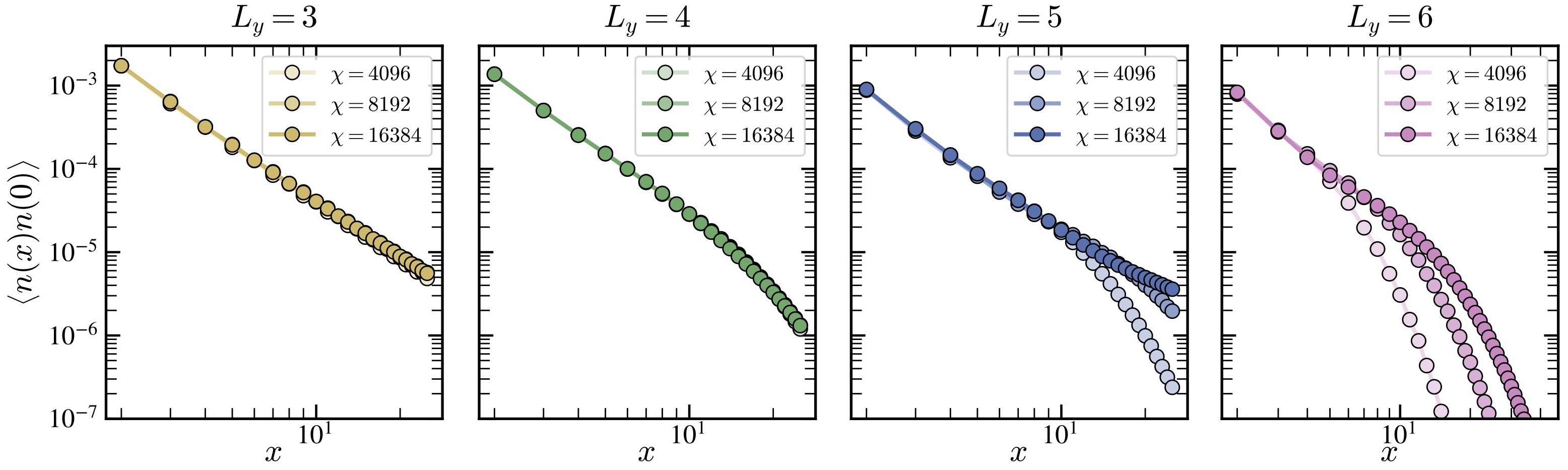
Figure S2: Density-density connected correlations for each of the four studied circumferences $L_{y}=3$ to $6$, with the Hubbard interaction tuned to the values at which the correlation length is maximal at the largest available bond dimension, namely $U(L_{y}=3)=11.125$, $U(L_{y}=4)=11.0$, $U(L_{y}=5)=11.6$, and $U(L_{y}=6)=11.4$, respectively. The even-circumference cylinders are threaded with $\Phi_{\text{ext}}=\pi/2$, as in the main text.

When $L_{y}$ is even, the Hamiltonian can be restored by composing the bare $T_{x}$ with a large gauge transformation. In contrast, by Fig. S1(b), we know that the effect of translations on the fluxes through loops cannot be gauged away when $L_{y}$ is odd. This manifests in the fact that $T_{x}^{\text{mag}}$ [see Eq. (48)] is ill-defined, which we see by imposing periodic boundary conditions and comparing $\bm{r}+L_{y}\bm{a}_{2}$ with $\bm{r}$; note that

$$\exp\left(\frac{i}{2}\bm{b}_{2}\cdot(\bm{r}+L_{y}\bm{a}_{2})\right)=\exp\left(i\pi L_{y}\right)\exp\left(\frac{i}{2}\bm{b}_{2}\cdot\bm{r}\right)\neq\exp\left(\frac{i}{2}\bm{b}_{2}\cdot\bm{r}\right).$$ (73)

SIII.2 Particle-hole

Now, let’s fix $\Phi_{\text{par}}=2\Phi_{\triangle}=+\pi$ and interrogate whether placing the system on a YC cylinder changes this conclusion. Focusing on a particular ring $r$ around the cylinder with flux $\Phi_{r},$ we note that

$$\tilde{\mathcal{\mathcal{P}}}:\Phi_{r}\mapsto\begin{cases}-\Phi_{r}&L_{y}\text{ even},\\ -\Phi_{r}+\pi&L_{y}\text{ odd}.\end{cases}$$ (74)

Therefore, $\tilde{\mathcal{\mathcal{P}}}$ is a symmetry (up to a gauge transformation) when

$$\Phi_{r}\in\begin{cases}\pi\mathbb{Z}&L_{y}\text{ even},\\ \frac{\pi}{2}+\pi\mathbb{Z}&L_{y}\text{ odd},\end{cases}$$ (75)

for all rings $r.$

When $L_{y}$ is even, Gauss’s law dictates that the flux $\Phi_{r_{1,2}}$ through two adjancent rings $r_{1,2}$ must be equal — note that this allows $T_{x}$ to be a symmetry (up to a gauge transformation). Therefore, possibly after threading $\phi$ external flux through each ring of the cylinder, it is possible to tune all the $\Phi_{r}$ simultaneously (to $0$ or $\pi$) so that $\tilde{\mathcal{\mathcal{P}}}$ is respected. Only in those cases is $T_{x}\tilde{\mathcal{\mathcal{P}}}$ also a symmetry (up to gauge).

On the other hand, when $L_{y}$ is odd, Gauss’s law instead dictates that

$$\Phi_{r_{2}}-\Phi_{r_{1}}=\pi\qquad\text{mod }2\pi.$$ (76)

This always rules out $T_{x}$ as a symmetry. However, so long as $\Phi_{r_{1}}$ is $\pi/2$ or $-\pi/2,$ both Eqs. (75) and (76) can be respected, so that $\tilde{\mathcal{\mathcal{P}}}$ is a symmetry (up to gauge). However, odd $L_{y}$ is special in that if we tune $\Phi_{r_{1}}$ to 0 or $\pi,$ then $T_{x}\tilde{\mathcal{\mathcal{P}}}$ is a symmetry (up to gauge) even though neither $T_{x}$ nor $\tilde{\mathcal{\mathcal{P}}}$ are themselves symmetries.

Appendix D Observable and Correlation Functions

SI Heisenberg Operator in terms of Fermions

If the sites are spinless FermionSites and up and down spins are encoded in adjacent FermionSites, we can compute spin correlations indirectly using the fermion creation and annihilation operators. Since the spin correlation operator $\vec{S}_{i}\cdot\vec{S}_{j}$ involves the product of two spin operators, we need to express it in terms of the fermion operators. In a system with spinless FermionSites, we can define the spin operators as:

$$S_{i}^{+}=c_{i\uparrow}^{\dagger}c_{i\downarrow},\quad S_{i}^{-}=c_{i\downarrow}^{\dagger}c_{i\uparrow},\quad S_{i}^{z}=\frac{1}{2}(c_{i\uparrow}^{\dagger}c_{i\uparrow}-c_{i\downarrow}^{\dagger}c_{i\downarrow}),$$ (77)

where $c_{i\uparrow}^{\dagger}$ creates an up-spin fermion on site $i$ and $c_{i\downarrow}^{\dagger}$ creates a down-spin fermion on site $i$. The spin correlation operator $\vec{S}_{i}\cdot\vec{S}_{j}$ can be written in terms of these fermion operators as:

$$\vec{S}_{i}\cdot\vec{S}_{j}=\frac{1}{2}\left(c_{i\uparrow}^{\dagger}c_{i\downarrow}c_{j\downarrow}^{\dagger}c_{j\uparrow}+c_{i\downarrow}^{\dagger}c_{i\uparrow}c_{j\uparrow}^{\dagger}c_{j\downarrow}\right)+S_{i}^{z}S_{j}^{z}.$$ (78)

SII Staggered Heisenberg Order Parameter

Here we express the staggered-Heisenberg order parameter in the hybrid $(x,k_{y})$ operator representation, where $x$ indexes cylinder rings. Because of translation invariance around the cylinder, it is useful to define the $y$-averaged inter-ring NN Heisenberg operator

$$\mathcal{O}_{\text{H}}(x)=\frac{1}{L_{y}}\sum_{y}\sum_{a=x,y,z}S^{a}(x,y)S^{a}(x+1,y),$$ (79)

where

$$S^{a}(x,y)=c^{\dagger}(x,y)\frac{\sigma^{a}}{2}c(x,y)=\frac{1}{L_{y}}\sum_{k,k^{\prime}}e^{i(k-k^{\prime})y}c^{\dagger}(x,k)\frac{\sigma^{a}}{2}c(x,k^{\prime}).$$ (80)

Since both the IQH and CSL ground states exhibit a two-ring translation invariance (i.e., are invariant under $(T_{x})^{2}$ in addition to $T_{y}$) then we can measure the local order parameter

$$\mathcal{O}^{\delta\text{Heis}}_{0}=\mathcal{O}_{\text{H}}(1)-\mathcal{O}_{\text{H}}(0).$$ (81)

In general, the hybrid representation reads

$$\mathcal{O}_{\text{H}}(x) =\frac{1}{L_{y}}\sum_{y}\sum_{a=x,y,z}S^{a}(x,y)S^{a}(x+1,y)$$

$$=\frac{1}{L_{y}^{2}}\sum_{a=x,y,z}\sum_{k,k^{\prime}}\sum_{p,p^{\prime}}\left(\frac{1}{L_{y}}\sum_{y}e^{i(k-k^{\prime}+p-p^{\prime})y}\right)c^{\dagger}(x,k)\frac{\sigma^{a}}{2}c(x,k^{\prime})\cdot c^{\dagger}(x+1,p)\frac{\sigma^{a}}{2}c(x+1,p^{\prime})$$

$$=\frac{1}{L_{y}^{2}}\sum_{a=x,y,z}\sum_{k,k^{\prime}}\sum_{p,p^{\prime}}c^{\dagger}(x,k)\frac{\sigma^{a}}{2}c(x,k^{\prime})\cdot c^{\dagger}(x+1,p)\frac{\sigma^{a}}{2}c(x+1,k-k^{\prime}+p).$$

Appendix E Correlation Lengths

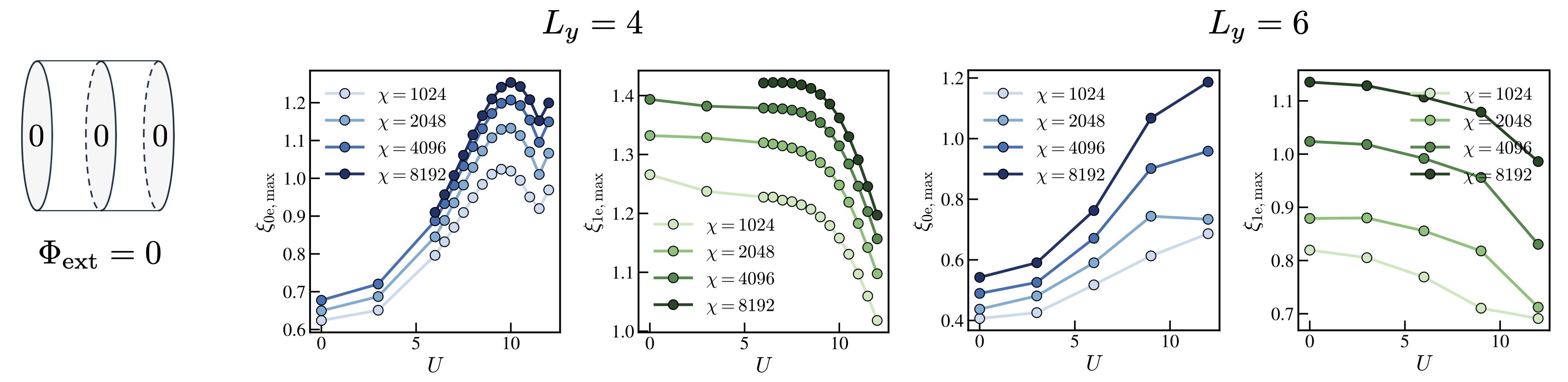
Figure S3: Correlation length data for even-circumference geometries. Left panel: Illustration of the external magnetic flux penetrating each loop of the infinite cylinder, namely no flux, $\Phi=0$. Center panels: Maximum correlation length at $L_{y}=4$ in the $Q=0e$ charge sector [blue] for a range of bond dimensions increasing with increasing darkness; and in the $Q=1e$ charge sector [green]. Right panel: The same for $L_{y}=6$.

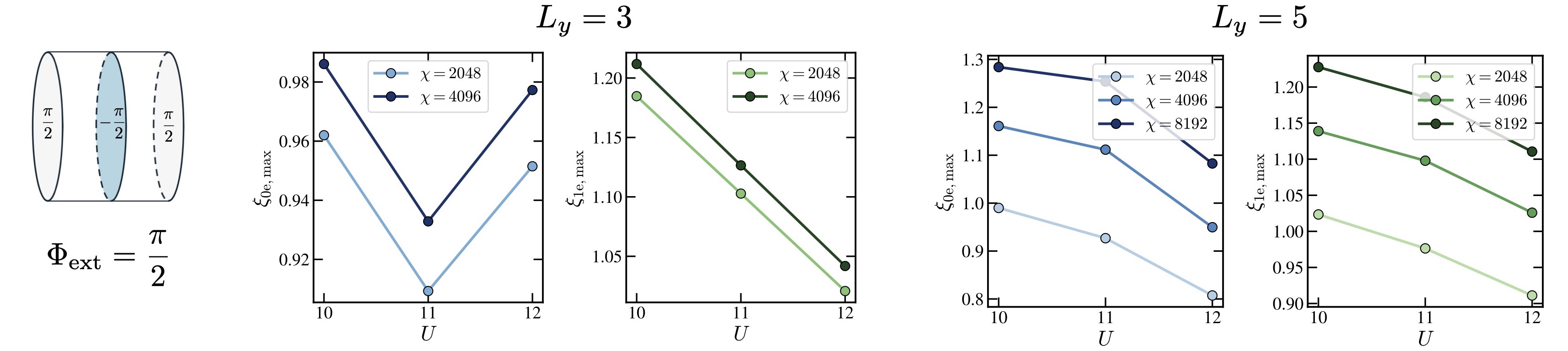
Figure S4: Correlation length data for even-circumference geometries. Left panel: Illustration of the external magnetic flux penetrating each loop of the infinite cylinder, which alternates between $\pm\pi/2$, corresponding to threaded flux $\Phi_{\text{ext}}=\pi/2$ in our conventions. Center panels: Maximum correlation length at $L_{y}=3$ in the $Q=0e$ charge sector [blue] for a range of bond dimensions increasing with increasing darkness; and in the $Q=1e$ charge sector [green]. Right panel: The same for $L_{y}=5$.

Here we briefly comment on additional data concerning the correlation lengths for geometries not displayed in the text. In particular, Fig. S3 shows correlation length data for the $L_{y}=4$ and $6$ cylinders which are threaded by no external flux. In particular, $L_{y}=6$ reproduces the behavior presented in Kuhlenkamp et al., [11]. We remark that the correlation lengths are quantitatively smaller than those at $\Phi_{\text{ext}}$ external flux, which are shown in the main text. We similarly show data for the $L_{y}=3$ and $5$ cylinders threaded by $\Phi_{\text{ext}}=\pi/2$ external flux. Unlike at $\Phi_{\text{ext}}=0$ in the main text, the flux breaks the glide-PH symmetry, and thus we see no diverging or quantitatively large correlation length (as is consistent with no spontaneous symmetry breaking).

Appendix F Correlation Length Extrapolation

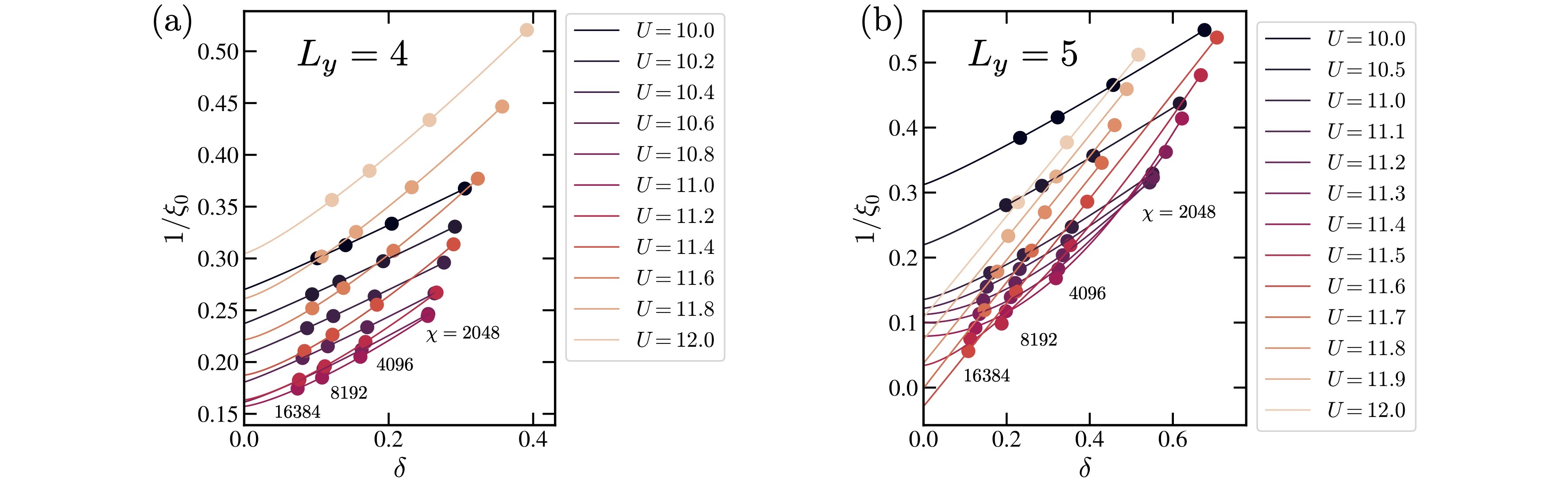
Figure S5: (a) Extrapolated inverse correlation length in the charge-neutral sector at $L_{y}=4$ and $\Phi_{\text{ext}}=\pi/2$ obtained following the method in Ref. [52], as detailed in Sec. F, for a range of Hubbard strengths [different colors] and for a sequence of increasing bond dimensions [same-colored points moving sequentially to the left]. The extrapolated inverse correlation length saturates at a minimum value exceeding $0.15$; the correlation length is equivalently bounded above by $6.6$ ring spacings. (b) The same for $L_{y}=5$ and $\Phi_{\text{ext}}=0$. In this case, the extrapolated inverse correlation length reaches and descends beyond 0, signaling the need for larger bond dimensions to accurately estimate large correlation lengths.

To obtain the extrapolated correlation lengths shown in the main text, we employ a recently-developed method for extrapolating correlation lengths in DMRG [52, 59]. Namely, we compute several of the largest eigenvalues of the transfer matrix $TX_{i}=\lambda_{i}X_{i}$ in the electric charge $Q_{E}=1$ sector for each $k_{y}$, and select those from the same “excitation branch” [52], namely carrying a consistent complex phase. These are related to the correlation lengths as

$$\epsilon_{i}=1/\xi_{i}=-\log\left|\lambda_{i}\right|$$ (82)

with $\epsilon_{i}\leq\epsilon_{i+1}$. We report $\xi$ in units of cylinder rings, or equivalently $u=a\sqrt{3}/2$ where $a$ is the lattice spacing of the underlying triangular lattice. Correspondingly, $\epsilon$ is reported in units of $u^{-1}$. For a system that is gapped in a charge sector $q=(Q,S_{z},k_{y})$, both $\epsilon_{1}^{q},\epsilon_{2}^{q}$ converge to the same infinite value as $\chi\to\infty$, namely the finite inverse correlation length. As a result, the quantity

$$\delta^{q}=\epsilon_{2}^{q}-\epsilon_{1}^{q}$$ (83)

vanishes at $\chi\to\infty$, serving as a good “scaling variable” that measures the deviation from convergence. To estimate $\xi(\chi\to\infty)$, we therefore compute $\epsilon(\delta)$ at each available $\epsilon(\chi),\delta(\chi)$ and extrapolate to $\delta=0$ with a polynomial fit, namely

$$\epsilon(\delta)=a+b\delta^{c}.$$ (84)

This extrapolation is shown in Fig. S5 for both $L_{y}=4$ at $\Phi_{\mathrm{ext}}=\pi/2$ and $L_{y}=5$ at $\Phi_{\mathrm{ext}}=0$, yielding the extrapolated values shown in the main text. In both cases, the correlation length is computed in the $(Q,S_{z},k_{y})=\bm{0}$, which hosts largest correlation length.

Appendix G Density-density correlations at all circumferences

Figure S6: Density-density connected correlations for each of the four studied circumferences $L_{y}=3$ to $6$, with the Hubbard interaction tuned to the values at which the correlation length is maximal at the largest available bond dimension, namely $U(L_{y}=3)=11.125$, $U(L_{y}=4)=11.0$, $U(L_{y}=5)=11.6$, and $U(L_{y}=6)=11.4$, respectively. The even-circumference cylinders are threaded with $\Phi_{\text{ext}}=\pi/2$, as in the main text.

In Fig. S6 we show the ring-averaged density-density connected correlations, defined as $\langle n_{\text{av}}(x)n_{\text{av}}(0)\rangle,$ where

$$n_{\text{av}}(x) =\frac{1}{L_{y}}\sum_{y}c^{\dagger}(x,y)c(x,y)=\frac{1}{L_{y}}\sum_{k}c^{\dagger}(x,k)c(x,k).$$ (85)

Panels (a,c), which correspond to the odd circumferences $L_{y}=3,5$ respectively, exhibit apparently algebraic correlations at long distances. On the other hand, panels (b,d) exhibit exponentially-decaying correlations that nonetheless feature a near-algebraic plateau, over a range of $x$ less than their respective correlation lengths.