A model-independent measurement of the expansion and growth rates from BOSS using the FreePower method

Abstract

In this work we provide a data analysis of the BOSS galaxy clustering data with the recently proposed FreePower method, which adopts as parameters the power spectrum band-powers instead of a specific cosmological parametrization. It relies on the Alcock-Paczyński effect and redshift-space distortions, and makes use of one-loop perturbation theory for biased tracers. In this way, we obtain for the first time constraints on the linear growth rate, on the Hubble parameter, as well as on various bias functions, that are independent of a model for the power spectrum shape and thus of both the early and late-time cosmological modelling. We find at $z_{\rm eff}=0.38$, $f=0.60^{+0.11}_{-0.09}$, $H/H_{0}=1.052^{+0.060}_{-0.041}$, and at $z_{\rm eff}=0.61$, $f=0.69^{+0.14}_{-0.13}$, $H/H_{0}=1.36\pm 0.10$. The low-$z$ $H/H_{0}$ result is at over 2$\sigma$ tension with Planck 2018 $\Lambda$CDM results. The precision in these results demonstrates the capabilities of the FreePower method. We also get constraints on the bias parameters which are in agreement with constraints from previous BOSS analyses, which serves as a cross-check of our pipeline.

1 Introduction

Ongoing surveys will soon provide extensive datasets probing the distribution of galaxies on very large volumes. Important ground surveys (DESI [1, 2], 4MOST [3], J-PAS [4], Vera C. Rubin Observatory LSST [5]) and space surveys (Euclid [6, 7], Nancy Grace Roman Space Telescope [8, 9]) of the large-scale structure (LSS) of the Universe are already underway or scheduled to commence shortly. The corresponding increase in precision of these surveys calls for an accurate theoretical modeling.

As it has become clear in last decade or so, a treatment using linear cosmological perturbation theory is no longer sufficient to optimize the science return [10]. An understanding of the non-linear formation of structures and the astrophysical uncertainties is necessary to use the observational data in the best possible way [11]. Perturbation theory provides the means to investigate LSS observables in the weakly non-linear regime. A comparison between the model predictions from non-linear perturbation theory and survey data can therefore lead to new insights. The theoretical higher-order power spectrum that we employ in this work has been derived within the context of the Effective Field Theory of the Large Scale Structure (EFTofLSS) [12, 13, 14, 15] (see also [16, 17] for the bispectrum and [18, 19, 20, 21] for non-standard cosmologies). EFTofLSS makes it possible to absorb the short-distance physics, which is not known in detail [11], into a set of parameters which can then be fitted to data. For an alternative approach based on Kinetic Field Theory, see e.g. [22].

The EFTofLSS studies fluctuations in the density of biased tracers, such as galaxies. Its natural cutoff lies at a scale where the gravitational evolution becomes highly non-linear and the impact of astrophysical processes becomes very high. Below the cutoff, EFT provides a connection between the initial conditions after inflation and the observables in the late Universe [10].

Complementing the EFTofLSS treatment, the impact of small-scale physics on the long-wavelength fluctuations can be modeled by ultraviolet (UV) counterterms [14]. They are also necessary because the short-scale physics is not modeled by perturbation theory. Moreover, infrared (IR) resummation [23] has to be applied to account for the fact that the shape of the baryon acoustic oscillation (BAO) peak is very sensitive to long-wavelength modes (bulk flows), which cannot be treated perturbatively either. Furthermore, to establish a connection between the theoretical modeling of the dark matter density contrast and the observables, it becomes necessary to consider the galaxy bias [24]. This provides a connection between the dark matter density field and the galaxy number density field, and redshift space distortions (RSD) [25], which account for the fact that the galaxies have a peculiar velocities due to clustering dynamics.

Most cosmological analyses of real data assume a (standard or non-standard) cosmological model in the theoretical description (see in particular [14, 17, 15] for the BOSS data). However, the results one gets are bound to depend on the underlying cosmological model, and cannot be employed to test different scenarios. It is therefore desirable to pursue an alternative route in order to remain as model-independent as possible [26, 27, 28, 29]. In this way, one reduces the chances to miss new physics or to introduce biases in the parameter estimation.

An approach to remain model independent, which was recently proposed in [27, 29, 30], consists in dividing the linear matter power spectrum $P(k)$ into several $k$-bins whose values are free to vary. From these bins, and a set of bias and counterterm parameters, the non-linear galaxy power spectrum and bispectrum are derived, allowing comparisons with the galaxy survey data. In this case, it is not necessary to make assumptions about the shape of $P(k)$. The non-linear correction to one loop in the power spectrum are evaluated assuming very general kernels, derived under the assumption of a homogeneous and isotropic background and the equivalence principle of general relativity, which implies that one can remove a pure-gradient metric perturbation by going to the free-falling frame of comoving observers [24]. All the parameters are left free to vary in each redshift. In this way, the results are independent of the details of both early-time models (that determine the initial power spectrum shape) and late-time models (that determine the background and perturbations growth). In Ref. [30] this framework was denoted as the FreePower method.

The growth rate $f$ should also be binned in $k$-space since in several modified gravity models it depends on $k$ but for this first real-data analysis this proves too demanding and for simplicity we assume the growth to be scale independent, in line with most similar analyses. In Ref. [29] we have shown that if $f$ depends on $k$ then one needs at least three multipoles to apply our methodology and recover all the parameters. One can show that taking $f$ to be $k$-independent, two multipoles are sufficient, which simplifies our analysis.

An interesting aspect of the FreePower method is that we can measure the dimensionless expansion rate $E$ and dimensionless angular diameter distance $L_{A}$, defined respectively by

$$E\equiv H(z)/H_{0}\,,\qquad L_{A}\equiv H_{0}D_{A}(z)\,,$$ (1.1)

independently of a model for the background or for the power spectrum shape. This is possible because both the power spectrum and bispectrum are distorted by the Alcock-Paczyński (AP) effect [31, 15] in a way that depends on $E,L_{A}$ (see Appendix C for more information). Another remarkable aspect of FreePower is that although the linear bias $b_{1}$ and the growth rate $f$ are degenerate with the linear spectrum shape $P(k)$, this degeneracy is broken at the non-linear level. The same occurs for $E$ and $L_{A}$. Using this we have shown, in particular, how FreePower can, without assuming any specific cosmological model, estimate the spatial curvature [32], or be combined with supernova and gravitational wave distances to test for the presence of modified gravity or cosmic opacity [33].

To obtain constraints on the various cosmological and bias parameters using observational data, we make use of Markov Chain Monte Carlo (MCMC) methods. A fast numerical evaluation of the non-linear galaxy power spectrum at the next to leading order (i.e. the one-loop order) is necessary for this procedure. This can be achieved with the FFTLog method [34], where the linear $P(k)$ is expanded as a superposition of power-law functions. The loop calculations can then be done analytically. An implementation of this method is provided by the code PyBird [35].

The main aim of this work is to produce the first real-data analysis with the FreePower framework using data from the Baryon Oscillation Spectroscopic Survey (BOSS). We do not strive for the best possible precision in this first real-data application of FreePower. Instead we focus on demonstrating that the method works and is able to produce competitive constraints for the $E(z)$ and $f(z)$. Since each likelihood evaluation is expensive and, as discussed below, we will have 17 free parameters, we had difficulty achieving convergence of the MCMC chains when using a small, 256-core computing cluster. We thus adopted three main simplifications in order to reduce the total computational time and get reliable results in a reasonable amount of time. First, we do not include the bispectrum, which if included would result in increased precision [30]. Second, we adopt the analytical kernels for an Einstein-deSitter (EdS) model. EdS kernels should in any case be a very good approximation for cosmologies that do not depart too much from $\Lambda$CDM; they have been adopted also in a previous analysis of BOSS data that we will compare to [14]. Finally, we include an informative distance prior, which we chose as Gaussians with $3\%$ standard deviations centered on the best-fit Planck $\Lambda$CDM values for each redshift bin.

With the above simplifications we obtained competitive constraints on cosmological and non-cosmological parameters. In particular, we are able to measure the dimensionless expansion rate and the growth function at both BOSS redshifts. This study also paves the way for model-independent analyses of future observational data of the LSS.

2 The FreePower model-independent approach

The theoretical model for the the galaxy density field power spectrum is given as [14, 35]

$$P_{\rm gg}(k,\mu,z)=P_{\rm 11}(k,\mu,z)+P_{\rm 22}(k,\mu,z)+P_{\rm 13}(k,\mu,z)+P_{\rm ctr}(k,\mu,z)+P_{\rm shot}.$$ (2.1)

This spectrum includes several free bias parameters [36], denoted $b_{1}$, $b_{2}$, $b_{\mathcal{G}_{2}}$, and $b_{\Gamma_{3}}$, and two counterterm parameters $c_{0},c_{2}$. In Ref. [30] we also included an overall smoothing factor that takes into account the Finger-of-God effect and the redshift uncertainty; we found however that the effect of this smoothing was subdominant and here, therefore, for simplicity, we do not include it. More details can be found in Appendix C. We explore the 17-dimensional parameter space with the Python MCMC code emcee [37].

In the model-independent approach presented here the linear matter power spectrum is parametrized in $k$-bins and the waveband values are varied in the MCMC. We select the values of $P_{L}$ at the central $k$-values

$$\{0.0001,0.003,0.023,0.079,0.187,0.364,0.630,1.0\}\,\,h/{\rm Mpc}.$$ (2.2)

Previous tests indicate that neither the exact spacing nor the number of the $k$-bins has a strong influence on the results on the other parameters [38]. The linear matter power spectrum is constructed with these varied parameters and a cubic spline interpolation between them. Because of that, the linear matter power spectrum is quite smooth. Therefore, the coupling between the large-scale IR modes and the mildly non-linear modes is rather weak [10] and the effect of IR resummation is in general small. In this approach we do not disentangle the growth factor $G(z)$ from the linear power spectrum, so we in fact measure $P_{L}(k,z)=G(z)^{2}P_{L}(k)$ at each redshift bin.

In the present analysis, we do not use the hexadecapole because it has been shown that the signal-to-noise ratio in the hexadecapole is very low compared to monopole and quadrupole [36]. Therefore, the model prediction for the hexadecapole is set to zero. However, due to the fact that at most monopole and quadrupole are considered in the likelihood in the final analysis, this simplification can only influence the possible coupling between multipoles through the wide-angle effects [39] and this effect should be small. For the data comparison, the $k$-range is restricted to $0.01\,h/{\rm Mpc}<k<0.3\,h/{\rm Mpc}$.

The bias parameters $b_{1}$, $b_{2}$, and $b_{\mathcal{G}_{2}}$ are left free to vary, together with the counterterm parameters $c_{0}$ and $c_{2}$. The bias parameter $b_{\Gamma_{3}}$ is set to zero, following [14], since it was observed that it is degenerate with the counterterm parameters and $b_{\mathcal{G}_{2}}$. The parameter $c_{4}$ need not be considered since we do not use the hexadecapole here. The parameters are in the so-called EC basis [36]. We also vary the growth rate $f$ and the dimensionless shot noise parameter

$$s=P_{\rm shot}\bar{n}-1\,,$$ (2.3)

where $\bar{n}\approx 3\times 10^{-4}(h/{\rm Mpc})^{3}$ [14] is the number density of the galaxies in BOSS.

2.1 Likelihood

For every set of parameters, the multipoles of the galaxy power spectrum according to the model can now be calculated. To compare the model to the data, we employ the likelihood [39]

$$\mathcal{L}\propto\exp[-\frac{1}{2}(\mathbf{P}_{\rm dat}-WM\mathbf{P}_{\rm theo})^{T}C^{-1}(\mathbf{P}_{\rm dat}-WM\mathbf{P}_{\rm theo})\bigg{]}\,.$$ (2.4)

$\mathbf{P}_{\rm dat}$ contains the data for the power spectrum multipoles $l=0,1,2,3,4$ in the $k$-range $0-0.4\,h/{\rm Mpc}$ in bins of $0.01\,h/{\rm Mpc}$. It has a vector of length $200$, combining these five multipoles and 40 $k$ bins. However, it is important to note that any analysis should be limited to $k<0.3\,h/{\rm Mpc}$ due to the Nyquist-frequency in the measured power spectra [39] and because the theoretical one-loop spectrum is hardly reliable at smaller scales. Therefore, we use $k_{\rm max}=0.3\,h/{\rm Mpc}$. $\mathbf{P}_{\rm theo}$ is a vector that contains the even multipoles of the model in $k$-bins of $0.001\,h/{\rm Mpc}$. $W$ is a 200$\times$2000 survey window function matrix and $M$ is the 1200$\times$2000 wide-angle transformation matrix [39]. We compare the theoretical predictions of the model to monopole and quadrupole of the data vector.

The covariance matrix $C$ is estimated from mock catalogs of BOSS DR12 [40, 39]. The Hartlap correction factor [41] is neglected here. It could affect the covariance matrix at the $\approx 1\%$ level [14]. Furthermore, one could perform a rescaling of parameter errors to account for a bias caused by the mock based covariance estimate [39, 42, 43]. However, this correction is at subpercent level too and is neglected here for simplicity.

2.2 Data sets from BOSS

parameter name	symbol	prior low-$z$ sample	high-$z$ sample
linear growth rate	$f$	${\cal U}[0,1]$	${\cal U}[0,1]$
dimensionless expansion rate	$E$	${\cal U}[0,2]$	${\cal U}[0,10]$
dim.less angular diameter distance	$L_{A}$	$\mathcal{N}(0.25,0.008)$	$\mathcal{N}(0.323,0.010)$
linear bias	$b_{1}$	$\mathcal{N}(1.67,0.36)$	${\cal U}[0,4]$
${\cal G}_{2}$ bias	$b_{\mathcal{G}_{2}}$	$\mathcal{N}(0.11,0.68)$	$\mathcal{N}(0,1)$
quadratic bias	$b_{2}$	$\mathcal{N}(-2.3,1.4)$	$\mathcal{N}(-3,2)$
dimensionless shot noise	$s$	$\mathcal{N}(0,0.5)$	$\mathcal{N}(0,0.5)$
counterterm (monopole)	$c_{0}/[{\rm Mpc}/h]^{2}$	$\mathcal{N}(-18.5,95.7)$	$\mathcal{N}(0,30)$
counterterm (quadrupole)	$c_{2}/[{\rm Mpc}/h]^{2}$	$\mathcal{N}(14.7,72)$	$\mathcal{N}(30,30)$
	$P_{1}/$$[{\rm Mpc}/h]^{3}$	$\mathcal{N}(429,42.9)$	$\mathcal{N}(429,42.9)$
	$P_{2}/$$[{\rm Mpc}/h]^{3}$	$\mathcal{N}(9870,987)$	$\mathcal{N}(9870,987)$
	$P_{3}/$$[{\rm Mpc}/h]^{3}$	$\mathcal{N}(23000,4000)$	$\mathcal{N}(23000,4000)$
linear power spectrum $k-$bins	$P_{4}/$$[{\rm Mpc}/h]^{3}$	$\mathcal{N}(8350,2000)$	$\mathcal{N}(8350,2000)$
	$P_{5}/$$[{\rm Mpc}/h]^{3}$	$\mathcal{N}(2320,800)$	$\mathcal{N}(2320,800)$
	$P_{6}/$$[{\rm Mpc}/h]^{3}$	$\mathcal{N}(911,500)$	$\mathcal{N}(911,500)$
	$P_{7}/$$[{\rm Mpc}/h]^{3}$	$\mathcal{N}(375,50)$	$\mathcal{N}(375,500)$
	$P_{8}/$$[{\rm Mpc}/h]^{3}$	$\mathcal{N}(100,20)$	$\mathcal{N}(100,200)$

Table 1: Free parameters used here in our model-independent approach, and their prior ranges in the MCMC analysis. We follow in part [36] in deciding the priors, adding a cut to the $P_{i}$ priors not to allow negative values.

We consider here data from the Baryon Oscillation Spectroscopic Survey (BOSS), which was part of the Sloan Digital Sky Survey (SDSS) III [44, 45]. It contains data on anisotropic galaxy clustering in Fourier space. The survey includes $1198006$ luminous galaxies over $10252$ ${\rm deg}^{2}$ [39]. The area is divided into the North Galactic Cap (NGC) and the South Galactic Cap (SGC). The data can be split into two redshift bins defined by $0.2<z<0.5$ and $0.5<z<0.75$. The values of the effective redshift are $z_{\rm eff}=0.38$ and $0.61$ [39]. We often refer to the samples simply as low-$z$ and high-$z$ survey, respectively.

The effective redshift can be used because the redshift bin is much smaller than the scale of variation of the growth factor $G(z)$ and the non-cosmological parameters. Therefore, the binning corresponds to evaluating all quantities at the same effective redshift [15]. Due to the time constraints on our available computing system, in this study only the (larger) NGC data set at both redshift bins is employed. More specifically, we compare our one-loop spectrum to the BOSS NGC monopole and quadrupole spectra.

The priors of the varied parameters are presented in Table 1. The priors on the eight parameters describing the linear matter power spectrum, as well as the bias parameters and counterterms were originally intended to be very broad and non-informative. However, the slow convergence of the chains prompted us to use tighter priors. For $P_{i}$ we decided to set them by running a MCMC with 256 walkers for 10000 steps for the high-$z$ case with flat $P$ priors and then doubling the standard deviation of the obtained posteriors for $P_{3}$-$P_{8}$ and adopting a tighter $10\%$ prior for $P_{1}$ and $P_{2}$ since those bins are on scales larger than the survey window. This is intended as a balance between using loose priors and helping MCMC convergence. As is shown in Appendix B, the $P_{3}$-$P_{8}$ priors remain considerably broader than the posteriors. For the shot-noise parameter, we adopt Gaussian priors which allows for a conservative 50% effective variation of the galaxy number density $\bar{n}$.

For the bias parameters, we left the priors very broad for high-$z$. For low-$z$, in order to see if convergence of the chain could be further improved, we used bias priors which were a bit tighter, while at the same time still broader than the likelihoods. We used as reference the final NGC low-$z$ posterior results from ISZ20. We took their errorbars, propagated the uncertainty in the power spectrum amplitude $A$ since they multiply all their bias parameters by $(A/A_{\rm Planck})^{1/2}$, symmetrized the results and multiplied them by a factor of two. We used the final results for the mean and standard deviation to construct our low-$z$ uncorrelated Gaussian priors. We also did the same for the counterterm parameters. We thus allow a twice larger uncertainty of ISZ20 in each bias and counterterm parameter as our prior. We also chose to adopt $10$ times tighter priors for the very small-scale bins $P_{7}$ and $P_{8}$ since these are beyond our 1-loop range and thus carry little information on $f$ and $E$. The Gaussian prior on $L_{A}(z)$ is centered around its Planck 2018 $\Lambda$CDM value (i.e. assuming $\Omega_{m0}=0.31$ so that $L_{A}=0.25$ for the low-$z$ and 0.323 for the high-$z$ sample) with a $3\%$ standard deviation. For $z\leq 1$ current constraints from Pantheon+ [46] are already at this level.

3 MCMC results

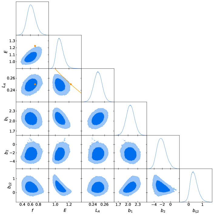
Figure 1: $68.3\%$ and $95.4\%$ highest-density confidence intervals corner plot for the cosmological and bias terms for the red low-$z$ sample ($z_{\rm eff}=0.38$). Orange dots mark the Planck 2018 $\Lambda$CDM values. The orange curve represents the $L_{A}$ vs. $E$ relation for $\Lambda$CDM for different values of $\Omega_{m0}$. $L_{A}$ results are prior-dominated.

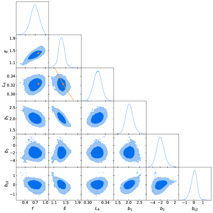
Figure 2: Same as Figure 1 for the high-$z$ sample ($z_{\rm eff}=0.61$).

We ran emcee using 256 walkers initialized in a small volume in parameter space. We ran, for each walker, 270k (180k) steps, for a total of 69 (46) million chain points for the low-$z$ (high-$z$) samples. Due to the complexity of the 1-loop calculations and the amount of MCMC steps needed, the total computational time used for both redshift bin runs was large, around 70000 CPU-hours. We analyzed the results using both the Python package getdist [47] and our own codes. The extra 50% points used in low-$z$ was to confirm that the results we found, which as we will discuss is in tension with $\Lambda$CDM CMB results, were robust. Indeed, the results adding these extra points changed little, which gives us confidence also in the convergence of our high-$z$ results.

Figures 1 and 2 show, for both redshift bins, the 68.3 and 95.4% confidence intervals (CI) for $f$, $E$, $L_{A}$ and the bias parameters. These are our main results. The orange dots mark the Planck 2018 values assuming flat $\Lambda$CDM [48], whereas the orange curves depict the $L_{A}(z)$ vs. $E(z)$ relation in flat $\Lambda$CDM when one varies the $\Omega_{m0}$ parameter. Interestingly, as can be seen, the $z_{\rm eff}=0.38$ result is in over 2$\sigma$ tension with flat $\Lambda$CDM, no matter what $\Omega_{m0}$ value is assumed. Beside the low-$z$ $E(z)$, all other parameters are mostly within 1$\sigma$ and always within 2$\sigma$ from Planck 2018 $\Lambda$CDM (except marginally for $P_{6},P_{7}$).

Tables 2 summarizes the marginalized constraints in each cosmological and bias parameter, whereas Table 3 show the results for all 8 $k$-bins of $P(k)$. Both tables also show the best-fit Planck 2018 values assuming flat $\Lambda$CDM.

The correlations $\rho$ among the 17 parameters are in most cases small. The average off-diagonal absolute value of $\rho$ is around 0.19 for both redshift bins. We list here some particular values for $z_{\rm eff}=0.38$ (0.61): $\rho(f,E)=0.59$ ($0.74$), $\rho(E,L_{A})=-0.28$ ($-0.27$), $\rho(E,b_{1})=-0.53$ ($-0.78$), $\rho(E,b_{\mathcal{G}_{2}})=-0.66$ ($-0.50$), $\rho(b_{\mathcal{G}_{2}},c_{2})=-0.79$ ($-0.19$). The full correlation matrices for both bins are shown in Appendix A.

One could worry that the informative prior we imposed on some of the parameters might have biased the low-$z$ results. Let’s dig deeper into this issue. First, the anti-correlation between $E,\,b_{1}$ (see Figures 6 and 8 in the appendices) means that a broader prior for $b_{1}$ could only allow larger values of $b_{1}$ and thereby increase the tension of $E$ with $\Lambda$CDM. The same holds true for $b_{{\cal G}_{2}}$, although the prior is less informative here. For $b_{2}$ the prior is the most informative and the correlation is positive ($\rho=0.33$), so a broader prior could allow for larger $b_{2}$, and in this case could indeed induce a higher $E$, alleviating the tension. However, the correlation is mild and our result for $b_{2}$ is in agreement with previous analyses of BOSS data [14, 17], so we do not expect that a broader prior would significantly affect the final constraints on $E$.

parameter	$z_{\rm eff}=0.38$	$z_{\rm eff}=0.61$	$\Lambda$CDM ($z=0.38$)	$\Lambda$CDM ($z=0.61$)
$f$	$0.60^{+0.11}_{-0.09}$	$0.69^{+0.14}_{-0.13}$	0.716	0.792
$E$	$1.052^{+0.060}_{-0.041}$	$1.36\pm{0.10}$	1.23	1.41
$L_{A}$	$0.248^{+0.008}_{-0.007}$	$0.323^{+0.009}_{-0.010}$	0.250	0.323
$b_{1}$	$2.08^{+0.12}_{-0.13}$	$2.03\pm 0.17$	–	–
$b_{2}$	$-2.4^{+1.1}_{-1.0}$	$-2.0^{+1.1}_{-1.0}$	–	–
$b_{\mathcal{G}_{2}}$	$0.33^{+0.28}_{-0.25}$	$0.07^{+0.31}_{-0.36}$	–	–
$c_{0}/[{\rm Mpc}/h]^{2}$	$-10^{+26}_{-36}$	$12\pm 18$	–	–
$c_{2}/[{\rm Mpc}/h]^{2}$	$27^{+23}_{-27}$	$26^{+21}_{-19}$	–	–
$s$	$0.26^{+0.48}_{-0.45}$	$0.14^{+0.43}_{-0.42}$	–	–

Table 2: Main results for the two redshift bins. We show best-fits with 68.3% CI. The last column shows the expected values for $\Lambda$CDM with Planck 2018 values [48].

	$P_{1}$	$P_{2}$	$P_{3}$	$P_{4}$	$P_{5}$	$P_{6}$	$P_{7}$	$P_{8}$
$k(h/$Mpc)	0.0001	0.003	0.023	0.079	0.187	0.364	0.630	1.0
$z_{\rm eff}=0.38$	$430^{+42}_{-44}$	$10200^{+760}_{-850}$	$22200^{+1900}_{-1600}$	$7990^{+760}_{-700}$	$2710^{+320}_{-340}$	$1070^{+220}_{-150}$	$366^{+45}_{-52}$	$101^{+19}_{-20}$
$z_{\rm eff}=0.61$	$431^{+41}_{-45}$	$9930^{+800}_{-850}$	$22500^{+1800}_{-1900}$	$8380^{+940}_{-850}$	$2310^{+380}_{-340}$	$950^{+220}_{-190}$	$480^{+160}_{-150}$	$110^{+91}_{-74}$
$\Lambda$CDM ref.	427	9980	23300	8560	2220	618	196	69.5

Table 3: Best-fit and 68.3% CI for each $k$-bin of the linear power spectrum (at $z=0$), in units of $({\rm Mpc}/h)^{3}$. The $k$ values represent the center of each $k$-bin. The model-independent constraints on $P_{i}(z)$ were converted to $z=0$ values for comparison using the $\Lambda$CDM growth factor $G(z)=0.818\hskip 5.69054pt(0.728)$ for $z=0.38\hskip 5.69054pt(0.61)$. The last row reports the corresponding Planck 2018 $\Lambda$CDM values as reference values.

We tested the convergence of our MCMC using primarly the auto-correlation time ($\tau$) estimates [37]. A large ratio between the number of steps and $\tau$ indicate that the chain ran for long enough to have a large effective number of independent steps. Ideally $\tau$ should converge to an asymptotic value for high enough number of steps. We found that around 200000 steps with each of 256 walkers were needed for reaching convergence. More details are provided in Appendix A. We also performed the Gelman-Rubin test [49]. This simple test is not the most reliable, specially using an ensemble sampler like emcee since in this approach the walkers are not independent. Nevertheless it gives another handle on convergence which is independent of the auto-correlation time analysis. For the cosmological parameters $f$, $E$ and $L_{A}$, we get $(\hat{R})^{(1/2)}=\{1.012,1.019,1.011\}$ for the low-$z$ run, and $(\hat{R})^{(1/2)}=\{1.071,1.091,1.027\}$ for the high-$z$ run. It is commonly assumed as a threshold for convergence the value $(\hat{R}_{\rm max})^{(1/2)}=1.1$. This agrees with the auto-correlation time results, which indicate good (reasonable) convergence for the low-$z$ (high-$z$) chains.

4 Comparison with previous analyses of BOSS data

In the following, the results obtained in this study are compared with the constraints previously obtained in model-dependent analyses. Is is important to note that the approaches applied in these analyses and the model-independent approach used here are quite different. An analysis of the nonlinear galaxy power spectrum obtained from BOSS under the model assumption of $\Lambda$CDM with varied neutrino masses was carried out in [14] (henceforth ISZ20). Another analysis of the BOSS data including information from power spectrum multipoles, the bispectrum monopole, the real-space power spectrum and the reconstructed power spectrum was carried out in [17] (henceforth, PI22). For each bias parameter, the authors report four results. Here we focus on the comparisons without the bispectrum and with a free spectral slope $n_{s}$.

par.	this work	ISZ20	PI22	this work	ISZ20	PI22
	$z_{\rm eff}=0.38$			$z_{\rm eff}=0.61$
$f$	$0.62\pm 0.10$	$0.735\pm 0.084$	—	$0.68\pm 0.13$	$0.750\pm 0.085$	—
$E$	$1.07\pm 0.05$	$1.136\pm 0.046$	—	$1.35\pm 0.10$	$1.384\pm 0.073$	—
$b_{1}$	$2.07\pm 0.13$	$1.67^{+0.16}_{-0.20}$	$2.21\pm 0.14$	$2.04\pm 0.17$	$2.28^{+0.22}_{-0.30}$	$2.33\pm 0.15$
$b_{2}$	$-2.2\pm 1.1$	$-2.3^{+0.5}_{-0.9}$	$-0.51^{+0.79}_{-0.97}$	$-1.9\pm 1.1$	$-2.7^{+0.5}_{-2.1}$	$-1.09^{+0.84}_{-1.0}$
$b_{\mathcal{G}_{2}}$	$0.39\pm 0.27$	$0.11^{+0.28}_{-0.40}$	$-0.38\pm 0.37$	$0.01^{+0.33}_{-0.35}$	$0.59^{+0.26}_{-0.08}$	$-0.19\pm 0.43$

Table 4: Comparison with the literature. Here we quote mean values and 68% percentiles using equal-tailed statistics, instead of highest-density values, since those are the ones reported in [17, 14] (we show the ISZ20 case with an $\omega_{b}$ prior).

A comparison of the inferred cosmological parameters with these works is given in Table 4. In this Table we quote mean values and 68% percentiles using equal-tailed statistics, instead of highest-density values, since those are the ones reported in ISZ20 and PI22. For the low-$z$ survey we find $f=0.62\pm 0.10$ and $E=1.07\pm 0.05$, in good agreement with $f=0.74\pm 0.08,E=1.14\pm 0.05$ from ISZ20. FreePower measures directly $f(z)$, while conventional analysis measure instead $f(z)\sigma_{8}(z)$. We therefore convert the latter using the values of $\sigma_{8}$ and $\Omega_{m0}$ obtained in ISZ20 and propagate the uncertainty in the integral for the growth factor. In Figure 3 we compare our results for $f(z)$ with ISZ20 and another previous analysis of BOSS and eBOSS galaxies [50] which assume $\Lambda$CDM. As can be seen, our model-independent results favor smaller values for $f$, which is in qualitative agreement with a recent analysis of the Planck 2018 data in a flat $\gamma\Lambda$CDM model, in which the growth-rate index $\gamma$, defined as $f\simeq\Omega_{m}(z)^{\gamma}$, was left free to vary [51].

We note that also the bias $b_{1},b_{2},b_{\cal G}$ agree to within 1$\sigma$ with ISZ20 and PI22. For the high-$z$ survey, we find $f=0.68\pm 0.13,E=1.35\pm 0.10$, again to within 1$\sigma$ from ISZ20 ($f=0.75\pm 0.08,E=1.38\pm 0.07$). Also the bias parameters are in 1$\sigma$ agreements.

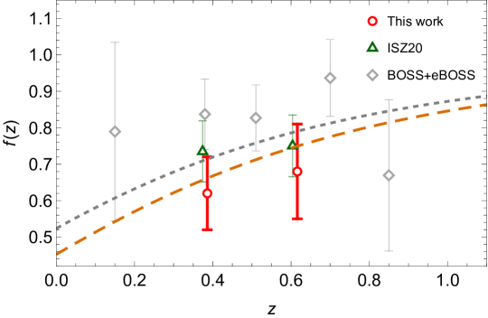
Figure 3: Comparison of our model-independent $f(z)$ results with those obtained assuming $\Lambda$CDM in ISZ20 and with BOSS+eBOSS galaxies [50]. FreePower measures directly $f(z)$ but conventional analysis measure instead $f(z)\sigma_{8}(z)$, so we convert the latter using the values of $\sigma_{8}$ and $\Omega_{m0}$ obtained in ISZ20. The best fit Planck 2018 curves are depicted in dashed gray ($\Lambda$CDM) or long-dashed orange ($\gamma\Lambda$CDM [51] – see text).

Our errors are in many cases comparable, but in some cases such as for $f$ and $E$ at $z_{\rm eff}=0.61$ they are between 30 and 50% larger than previous analyses based on $\Lambda$CDM. A smaller precision is of course entirely expected since our approach is more flexible and introduces more free parameters. We nevertheless find it noteworthy that the loss of precision is in general not very large, especially compared with the gains in robustness to modelling.

5 Comparison of distance measurements

Few methods are capable of direct measurements of the expansion rate (or of the corresponding Hubble distance) without an underlying assumption of the cosmological model. One such method relies on the use of the so-called cosmic chronometers (CC), which are based on modelling passively evolving galaxies. In Figure 4 we compare our results for $E(z)$ with a recently compiled catalog of CC [52]. For clarity, we only show the CC for $z<1.2$, but this CC dataset extends until $z\simeq 2$. Since CC measure $H(z)$ instead of $E(z)$, we convert their measurements using the value of $H_{0}=67.42\pm 4.75$, obtained from CC data itself with a Gaussian Process extrapolation [53]. As can be seen, our results are very competitive, and compensate the smaller number of data points with smaller error bars.

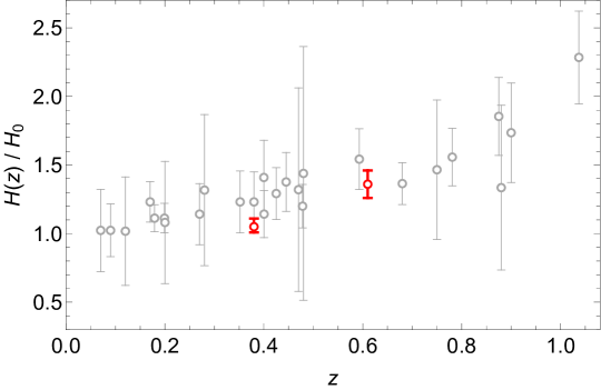
Figure 4: Comparison of $E(z)$ results using cosmic chronometers (CC, in gray) and our FreePower result (in red). For the CC data we use the compilation in [52], limited to $z<1.2$, and use the $H_{0}$ value obtained from CC data itself with a Gaussian Process extrapolation [53].

Recently, the first release of DESI data [54] was analysed and constraints have been put forward for $E$ and $L_{A}$ at seven redshift bins from 0.3 to 2.33 (effective values). To compare directly to DESI tables and figures, we first convert our $E,\,L_{A}$ constraints into the distance parameters $D_{H},\,D_{M}$ as

$$\frac{D_{M}}{r_{d}} =\frac{L_{A}(1+z)}{H_{0}r_{d}},\quad\frac{D_{H}}{r_{d}}=\frac{1}{H_{0}r_{d}E}\,,$$ (5.1)

and then into the basis employed by the DESI collaboration for some of their figures:

$$\frac{D_{V}}{r_{d}} =\frac{1}{r_{d}}\big{(}zD_{M}^{2}D_{H}\big{)}^{1/3},\quad F_{AP}=\frac{D_{M}}{D_{H}}\,,$$ (5.2)

where $r_{d}$ is the sound horizon measured on the CMB. When we tabulate our results for $D_{M}/r_{d},D_{H}/r_{d},D_{V}/r_{d}$ we adopt for $H_{0}r_{d}$ the best fit $\Lambda$CDM value of the DESI paper, namely

$$r_{d}h=\frac{r_{d}H_{0}}{100\,({\rm km/sec/Mpc})}=101.8\pm 1.3\,{\rm Mpc}\,.$$ (5.3)

This is however quite different from Planck result

$$r_{d}h=\frac{r_{d}H_{0}}{100\,({\rm km/sec/Mpc})}=98.82\pm 0.82\,{\rm Mpc}\,.$$ (5.4)

so the comparison of the $H_{0}r_{d}$-dependent quantities might be misleading. $F_{AP}$, on the other hand, is independent of $H_{0}r_{d}$. We also include the measurements obtained in ISZ20 with the $\alpha$-analysis, which is a more model-independent analysis of the BOSS data. In this section we always use the mean values and symmetric 68% percentiles.

The results are illustrated in Figure 5, which is to be compared with Fig. 1 of [54]. Since we find a value of $E$ two sigma below Planck $\Lambda$CDM for the low-$z$ sample, and therefore a larger $D_{H}$, we correspondingly find a $F_{AP}$ smaller, and a $D_{V}/r_{d}$ larger, than $\Lambda$CDM. For $F_{AP}$ the tension with the fiducial $\Lambda$CDM result at low-$z$ is around 2.9$\sigma$. Our results agree to within 1$\sigma$ with ISZ20. Interestingly, the deviation of $F_{AP}$ from $\Lambda$CDM we find at both redshift bins goes in the opposite direction with respect to the one detected by DESI in the intermediate sample at $z=0.51$. Table 5 summarizes all the distances.

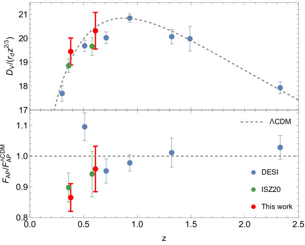
Figure 5: Top: Comparison of $D_{V}/r_{d}$ (rescaled by $z^{2/3}$ to match the DESI prescription) of DESI BAO (blue dots) and ISZ20 (green dots, slightly displaced for clarity) with our results (red dots). The dashed line is the best fit Planck 2018 $\Lambda$CDM curve. Bottom: same for $F_{AP}$ divided by the Planck 2018 $\Lambda$CDM $F_{AP}$ (note that in Ref. [54] $F_{AP}$ was normalized to the similar, but not identical, DESI $\Lambda$CDM best fit).

data		$z$	$D_{H}/r_{d}$	$D_{M}/r_{d}$	$\rho$	$D_{V}/(r_{d}z^{2/3})$	$F_{AP}/F^{\Lambda CDM}_{AP}$
		0.30	–	–	–	17.70$\pm$0.33	–
		0.51	21.0$\pm$0.6	13.62$\pm$0.25	-0.445	19.69$\pm$0.23	1.10$\pm$0.04
		0.71	20.1$\pm$0.6	16.85$\pm$0.32	-0.42	20.02$\pm$0.25	0.95$\pm$0.04
DESI		0.93	17.88$\pm$0.35	21.71$\pm$0.28	-0.389	20.85$\pm$0.18	0.98$\pm$0.03
		1.32	13.8$\pm$0.4	27.8$\pm$0.7	-0.444	20.07$\pm$0.30	1.01$\pm$0.05
		1.49	–	–	–	20.00$\pm$0.50	–
		2.33	8.52$\pm$0.17	39.7$\pm$0.9	-0.477	17.93$\pm$0.25	1.03$\pm$0.04
		0.38	26.2$\pm$1.3	9.9$\pm$1.3	–	18.86$\pm$0.28	0.90$\pm$0.05
ISZ20		0.61	21.5$\pm$1.3	14.1$\pm$1.3	–	19.70$\pm$0.4	0.94$\pm$0.07
		0.38	27.52$\pm$1.4	10.08$\pm$0.28	0.282	19.45$\pm$0.56	0.87$\pm$0.045
this	​​​​​ work	0.61	21.81$\pm$1.7	15.31$\pm$0.47	0.269	20.31$\pm$0.77	0.96$\pm$0.07

Table 5: Distance measurements in DESI, ISZ20, and this work.

6 Conclusions and outlook

The BOSS DR12 datasets at effective redshifts $0.38$ and $0.61$ for the NGC survey have been analyzed following, for the first time, the model-independent FreePower approach. The linear matter power spectrum has been parametrized in several $k$-bins and varied in the MCMC, along with the dimensionless expansion rate, the dimensionless angular diameter distance, the growth rate, and many other parameters that model the non-linear correction. It was shown that consistent results for various cosmological and non-cosmological parameters can be obtained from the observational data with only weak assumptions about the underlying cosmological model in terms of background expansion and power spectrum shape. The results obtained showcase the potential of model-independent analyses of galaxy surveys.

The main findings of this study are summarized below:

• We were able to constrain both non-cosmological parameters (bias, shot-noise and counterterm parameters), and cosmological parameters in a model-independent way using LSS surveys. In particular, we measured $f(z)$ and $E(z)$ at both BOSS redshift bins (Table 2).

• Our constraints are consistent with the ones from previous model-dependent analyses [14, 17]. In the case of the growth rate and the expansion rate, the uncertainties increase in the model-independent analysis, as expected due to it having fewer assumptions.

• For $z_{\rm eff}=0.38$, we find a tension at over $2\sigma$ with $\Lambda$CDM results for $E$, but not for the growth rate $f$. For $z_{\rm eff}=0.61$ we find good agreement with $\Lambda$CDM for both $E$ and $f$. For the bias parameters we find good agreement with a previous 1-loop analysis in both bins.

• We find a value of $F_{AP}$ in agreement with previous BOSS analyses. Our $F_{AP}$ for low-$z$ is in almost 3$\sigma$ tension with the fiducial Planck $\Lambda$CDM, and in the opposite way than the recent DESI estimate for the adjacent $z=0.51$ redshift bin.

This work demonstrates the possibility of implementing a theoretical model for non-linear structure formation together with the model-independent galaxy survey analysis approach. It paves the way for model-independent analyses of future observational data of the large-scale structure of the Universe. The estimates of $f,E,L_{A}$ can be employed to answer fundamental questions like the spatial curvature [32] or the cosmological Poisson equation [55] independently of the initial conditions (the power spectrum shape) and of the late-time evolution (expansion and growth rates).

There are of course many ways to extend our results in the future. In terms of data, the hexadecapole can be included in the analysis next to monopole and quadrupole. One can also include the bispectrum [56], which is of the same order as the one-loop power spectrum in the non-linear perturbation theory [17]. The BOSS SGC data can also be included, which would increase the effective volume of the sample by around 37% [14]. In terms of methodology, the growth rate $f(z)$ could be generalized to be scale-dependent, and/or one could try using a different number of $k$-bins. One could also use uninformative priors for the dimensionless distance $L_{A}$ to let it be constrained solely by the LSS data. Another possibility is to perform a combined analysis of both redshift bins, since in FreePower they share the same linear $P(k)$ parameters. In terms of theory, our analysis can be expanded by including deviations from the EdS kernels [57, 58, 59]. It can also be extended to include the peculiar-velocity power spectrum [27, 60, 61]. We note that a similar model-independent analysis can be carried out to investigate possible primordial non-Gaussianity (PNG) [16]. We plan to pursue these lines of investigation in future work.

Appendix A Correlations and convergence

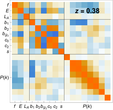
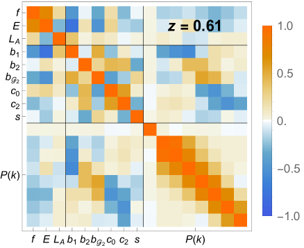
Figure 6: Correlation matrix for all 17 parameters in both redshift bins. The structure is similar in both bins; at low-$z$ the correlations among the bias parameters is slightly larger.

The correlation matrices among all 17 parameters are depicted in Figure 6, for both redshift bins. As discussed in the text, most terms are small. The bias parameters have stronger correlations among themselves for the lower redshift bin. The different $P(k)$ bins have strong positive correlations with their immediate neighbors, except when tight priors were used (this was the case for $P_{1}$ for both $z_{\rm eff}$ values, and for $P_{7}$ and $P_{8}$ for $z_{\rm eff}=0.38$). The data-driven cosmological parameters $f$ and $E$ are positively correlated among themselves and anti-correlated with $b_{1}$ and $b_{\mathcal{G}_{2}}$.

We also display the integrated autocorrelation times ($\tau$) in Figure 7. We compute $\tau$ for each walker individually and these estimates are averaged afterwards [37]. The MCMC shows clear signs of convergence as the estimates for the $\tau$ start crossing the dashed line.

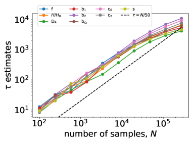
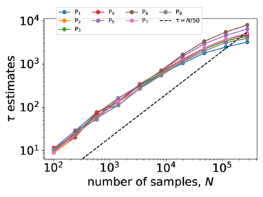
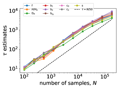
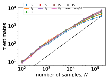
Figure 7: Integrated autocorrelation times as a function of the number of steps in each of the 256 walkers. Top: $z_{\rm eff}=0.38$; bottom: $z_{\rm eff}=0.61$.

Appendix B Full corner plots

Here we present larger triangle plots, which include more parameters and also the prior ranges. Figures 8 and 9 are extensions of Figure 1 and 2, including also the counterterm and shot-noise parameters. Figures 10 and 11 instead show the parameters depicting the power spectrum bins, together with the growth function and expansion rate, which are the two data-driven cosmological parameters.

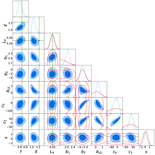
Figure 8: Similar to Figure 1 for $z_{\rm eff}=0.38$, but including counterterms and shot-noise parameters. The priors are depicted in red; the green points mark the Planck $\Lambda$CDM values.

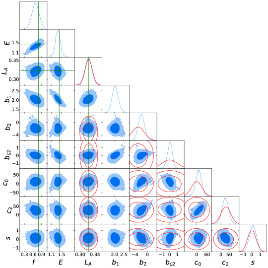
Figure 9: Same as Figure 8 for $z_{\rm eff}=0.61$.

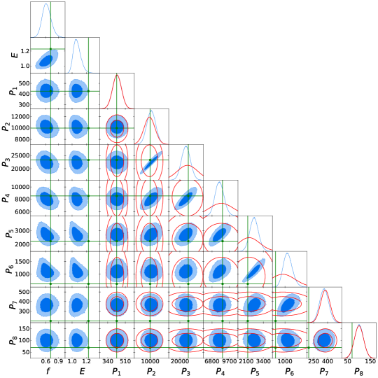
Figure 10: Same as Figure 9 for $z_{\rm eff}=0.38$ but for the parameters describing the cosmology and the linear matter power spectrum.

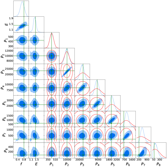
Figure 11: Same as Figure 10 for $z_{\rm eff}=0.61$.

Appendix C One-loop galaxy power spectrum

The one-loop corrections for the galaxy density field power spectrum take the form [14]

$$P_{11}(k,\mu,z)=\big{[}Z_{1}^{\rm sym}(\mathbf{k})\big{]}^{2}P_{\rm L}(k,z),$$ (C.1)

$$P_{22}(k,\mu,z)=2\int{\rm d}\mathbf{q}\big{[}Z_{2}^{\rm sym}(\mathbf{q},\mathbf{k}-\mathbf{q})\big{]}^{2}P_{\rm L}(q,z)P_{\rm L}(\absolutevalue{\mathbf{k}-\mathbf{q}},z)\$$ (C.2)

and

$$P_{13}(k,\mu,z)=6Z_{1}^{\rm sym}(\mathbf{k})\int{\rm d}\mathbf{q}\,Z_{3}^{\rm sym}(\mathbf{k},\mathbf{q},-\mathbf{q})P_{\rm L}(k,z)P_{\rm L}(q,z),$$ (C.3)

where $Z_{1}^{\rm sym}$, $Z_{2}^{\rm sym}$, and $Z_{3}^{\rm sym}$ are the symmetrized redshift space kernels for the galaxy density field.

The biased and RSD-corrected kernels are (see e.g. [14])

$$Z_{1}({\bf k})= \left(1+\mu^{2}\beta(k)\right)b_{1}\,,$$ (C.4)

$$Z_{2}(\mathbf{k}_{1},\mathbf{k}_{2})=\, b_{1}\bigg{\{}F_{2}(\mathbf{k}_{1},\mathbf{k}_{2})+\beta(k)\mu^{2}G_{2}(\mathbf{k}_{1},\mathbf{k}_{2})$$

$$+b_{1}\frac{\beta(k)\mu k}{2}\left[\frac{\mu_{1}}{k_{1}}\big{(}1+\beta(k_{2})\mu_{2}^{2}\big{)}+\frac{\mu_{2}}{k_{2}}\big{(}1+\beta(k_{1})\mu_{1}^{2}\big{)}\right]\bigg{\}}+\frac{b_{2}}{2}+b_{{\cal G}_{2}}S_{1}(\mathbf{k}_{1},\mathbf{k}_{2})\,,$$ (C.5)

(already symmetrized) and

$$Z_{3}(\mathbf{k}_{1},\mathbf{k}_{2},\mathbf{k}_{3})\!=\, b_{1}\bigg{\{}F_{3}(\mathbf{k}_{1},\mathbf{k}_{2},\mathbf{k}_{3})+\beta(k)\mu^{2}G_{3}(\mathbf{k}_{1},\mathbf{k}_{2},\mathbf{k}_{3})$$

$$\;+\!b_{1}\beta(k)\mu k\frac{\mu_{3}}{k_{3}}\Big{[}F_{2}(\mathbf{k}_{1},\mathbf{k}_{2})+\beta(k_{12})\mu_{12}^{2}G_{2}(\mathbf{k}_{1},\mathbf{k}_{2})\Big{]}$$

$$\;+\!b_{1}\beta(k)\mu k\big{(}1+\beta(k_{1})\mu_{1}^{2}\big{)}\frac{\mu_{23}}{k_{23}}G_{2}(\mathbf{k}_{2},\mathbf{k}_{3})\!+\!b_{1}^{2}\frac{\big{[}\beta(k)\mu k\big{]}^{2}}{2}\big{(}1+\beta(k_{1})\mu_{1}^{2}\big{)}\frac{\mu_{2}}{k_{2}}\frac{\mu_{3}}{k_{3}}\bigg{\}}$$

$$\!+2b_{{\cal G}_{2}}S_{1}(\mathbf{k}_{1},\mathbf{k}_{2}+\mathbf{k}_{3})F_{2}(\mathbf{k}_{2},\mathbf{k}_{3})+b_{1}b_{{\cal G}_{2}}\beta(k)\mu k\frac{\mu_{1}}{k_{1}}S_{1}(\mathbf{k}_{2},\mathbf{k}_{3})$$

$$\!+2b_{\Gamma_{3}}S_{1}(\mathbf{k}_{1},\mathbf{k}_{2}+\mathbf{k}_{3})(F_{2}(\mathbf{k}_{2},\mathbf{k}_{3})-G_{2}\big{(}\mathbf{k}_{2},\mathbf{k}_{3})\big{)}\,,$$ (C.6)

(to be symmetrized), where ${\bf k}={\bf k}_{1}+{\bf k}_{2}$ in $Z_{2}$ and ${\bf k}={\bf k}_{1}+{\bf k}_{2}+{\bf k}_{3}$ in $Z_{3}$, $\mu_{i}\equiv\mu({\bf k}_{i})$ ($i=1,\dots,3$) are the angle cosine between ${\bf k}$ and the line of sight, $k_{12}=|{\bf k}_{1}+{\bf k}_{2}|$, $\mu_{12}\equiv\mu({\bf k}_{12})$, and so on. $F_{2,3}$ and $G_{2,3}$ are the density and velocity kernels at second and third order, respectively, in standard perturbation theory.

The kernels have been derived for an Einstein-deSitter cosmology. They include three free $z$-dependent functions, denoted $b_{1}$, $b_{2}$, $b_{\mathcal{G}_{2}}$. The bias parameter $b_{\Gamma_{3}}$ is set to zero. The restriction to Einstein-deSitter is of course a break of the model-independence, although it is well-known that this approximation works very well also for $\Lambda$CDM and other cosmologies that do not depart too much from it. In our FreePower method the kernels have been implemented in a much more general way, under general conditions like equivalence principle and Galilean invariance, and can be considered essentially model-independent.

The counterterms can be parametrized as follows [62]:

$$P_{\rm ctr}(k,\mu,z)=-2\tilde{c}_{0}(z)k^{2}P_{\rm L}(z,k)-2\tilde{c}_{2}(z)f(z)\mu^{2}k^{2}P_{\rm L}(z,k).$$ (C.7)

The stochastic contribution to the power spectrum is modeled as a constant shot noise or Poisson noise. The number density in BOSS is $\bar{n}\approx 3\times 10^{-4}(h/{\rm Mpc})^{3}$ [14] which leads to a Poisson noise of $1/\bar{n}$. However, deviations from this value are possible through exclusion effects [63], and Therefore we include the variable shot-noise parameter defined in Eq. (2.3). The multipoles can be computed via

$$P_{{\rm gg},l}(z,k)\equiv\frac{2l+1}{2}\int_{-1}^{1}{\rm d}\mu\,P_{\rm gg}(k,\mu,z)\mathcal{P}_{l}(\mu),$$ (C.8)

where $\mathcal{P}_{l}(\mu)$ are the Legendre polynomials.

When the galaxy spectra are estimated from data, one has to assume a reference cosmology (fiducial cosmology). The fiducial cosmology, a flat $\Lambda$CDM cosmology with $\Omega_{m0}=0.31$, is used to convert observables (RA, DEC, $z$) into cartesian coordinates. Then, quantities like $k$, $\mu$, and volumes are computed assuming the reference cosmological model. The reference cosmology is different from the true cosmology and this difference leads to a geometrical distortion, the Alcock-Paczyński effect. The observable galaxy power spectrum is [14]

$$P_{\rm obs}(k_{\rm obs},\mu_{\rm obs})=P_{gg}\big{(}k_{\rm true}[k_{\rm obs},\mu_{\rm obs}],\mu_{\rm true}[k_{\rm obs},\mu_{\rm obs}]\big{)}\times\frac{L_{\rm A,fid}^{2}E_{\rm true}}{E_{\rm A,true}^{2}H_{\rm fid}}.$$ (C.9)

Here $k_{\rm obs}$ and $\mu_{\rm obs}$ are the quantities obtained under a given cosmological reference model. This is also the case for $L_{\rm A,fid}$ and $E_{\rm fid}$. To convert between the true quantities and the quantities derived in the reference model, it is necessary to know $E_{\rm true}$ and $L_{\rm A,true}$:

$$k_{\rm true}^{2}=k_{\rm obs}^{2}\Bigg{[}\bigg{(}\frac{E_{\rm true}}{E_{\rm fid}}\bigg{)}^{2}\mu_{\rm obs}^{2}+\bigg{(}\frac{L_{\rm A,fid}}{L_{\rm A,true}}\bigg{)}^{2}(1-\mu_{\rm obs}^{2})\Bigg{]},$$ (C.10)

$$\mu_{\rm true}^{2}=\bigg{(}\frac{E_{\rm true}}{E_{\rm fid}}\bigg{)}^{2}\mu_{\rm obs}^{2}\Bigg{[}\bigg{(}\frac{E_{\rm true}}{E_{\rm fid}}\bigg{)}^{2}\mu_{\rm obs}^{2}+\bigg{(}\frac{L_{\rm A,fid}}{L_{\rm A,true}}\bigg{)}^{2}(1-\mu_{\rm obs}^{2})\Bigg{]}^{-1}.$$ (C.11)

When the Alcock-Paczyński effect is considered as well, the expression becomes

$$P_{{\rm gg},l}(k)\equiv\frac{2l+1}{2}\int_{-1}^{1}{\rm d}\mu_{\rm obs}P_{\rm obs}(k_{\rm obs},\mu_{\rm obs})\mathcal{P}_{l}(\mu_{\rm obs}).$$ (C.12)

References

- [1] DESI collaboration, DESI 2024 III: Baryon Acoustic Oscillations from Galaxies and Quasars, 2404.03000.
- [2] DESI collaboration, DESI 2024 IV: Baryon Acoustic Oscillations from the Lyman Alpha Forest, 2404.03001.
- [3] R.S. de Jong, O. Agertz, A.A. Berbel, J. Aird, D.A. Alexander, A. Amarsi et al., 4MOST: Project overview and information for the First Call for Proposals, The Messenger 175 (2019) 3 [1903.02464].
- [4] S. Bonoli, A. Marín-Franch, J. Varela, H. Vázquez Ramió, L.R. Abramo, A.J. Cenarro et al., The miniJPAS survey: A preview of the Universe in 56 colors, A&A 653 (2021) A31 [2007.01910].
- [5] LSST Science Collaboration, P.A. Abell, J. Allison, S.F. Anderson, J.R. Andrew, J.R.P. Angel et al., LSST Science Book, Version 2.0, arXiv e-prints (2009) arXiv:0912.0201 [0912.0201].
- [6] L. Amendola, S. Appleby, A. Avgoustidis, D. Bacon, T. Baker, M. Baldi et al., Cosmology and fundamental physics with the Euclid satellite, Living Reviews in Relativity 21 (2018) 2 [1606.00180].
- [7] R. Laureijs, J. Amiaux, S. Arduini, J.L. Auguères, J. Brinchmann, R. Cole et al., Euclid Definition Study Report, arXiv e-prints (2011) arXiv:1110.3193 [1110.3193].
- [8] T. Eifler, M. Simet, E. Krause, C. Hirata, H.-J. Huang, X. Fang et al., Cosmology with the Roman Space Telescope: synergies with the Rubin Observatory Legacy Survey of Space and Time, MNRAS 507 (2021) 1514 [2004.04702].
- [9] B.M. Rose, C. Baltay, R. Hounsell, P. Macias, D. Rubin, D. Scolnic et al., A Reference Survey for Supernova Cosmology with the Nancy Grace Roman Space Telescope, arXiv e-prints (2021) arXiv:2111.03081 [2111.03081].
- [10] G. Cabass, M.M. Ivanov, M. Lewandowski, M. Mirbabayi and M. Simonović, Snowmass white paper: Effective field theories in cosmology, Phys. Dark Univ. 40 (2023) 101193 [2203.08232].
- [11] D. Green, J.T. Ruderman, B.R. Safdi, J. Shelton, A. Achúcarro, P. Adshead et al., Snowmass Theory Frontier: Astrophysics and Cosmology, arXiv e-prints (2022) arXiv:2209.06854 [2209.06854].
- [12] D. Baumann, A. Nicolis, L. Senatore and M. Zaldarriaga, Cosmological Non-Linearities as an Effective Fluid, JCAP 07 (2012) 051 [1004.2488].
- [13] J.J.M. Carrasco, M.P. Hertzberg and L. Senatore, The Effective Field Theory of Cosmological Large Scale Structures, JHEP 09 (2012) 082 [1206.2926].
- [14] M.M. Ivanov, M. Simonović and M. Zaldarriaga, Cosmological Parameters from the BOSS Galaxy Power Spectrum, JCAP 05 (2020) 042 [1909.05277].
- [15] G. D’Amico, J. Gleyzes, N. Kokron, K. Markovic, L. Senatore, P. Zhang et al., The Cosmological Analysis of the SDSS/BOSS data from the Effective Field Theory of Large-Scale Structure, JCAP 05 (2020) 005 [1909.05271].
- [16] G. Cabass, M.M. Ivanov, O.H.E. Philcox, M. Simonović and M. Zaldarriaga, Constraints on Single-Field Inflation from the BOSS Galaxy Survey, Phys. Rev. Lett. 129 (2022) 021301 [2201.07238].
- [17] O.H.E. Philcox and M.M. Ivanov, BOSS DR12 full-shape cosmology: CDM constraints from the large-scale galaxy power spectrum and bispectrum monopole, Phys. Rev. D 105 (2022) 043517 [2112.04515].
- [18] A. Chudaykin, K. Dolgikh and M.M. Ivanov, Constraints on the curvature of the Universe and dynamical dark energy from the Full-shape and BAO data, Phys. Rev. D 103 (2021) 023507 [2009.10106].
- [19] M.M. Ivanov, E. McDonough, J.C. Hill, M. Simonović, M.W. Toomey, S. Alexander et al., Constraining Early Dark Energy with Large-Scale Structure, Phys. Rev. D 102 (2020) 103502 [2006.11235].
- [20] W.L. Xu, J.B. Muñoz and C. Dvorkin, Cosmological constraints on light but massive relics, Phys. Rev. D 105 (2022) 095029 [2107.09664].
- [21] A. Laguë, J.R. Bond, R. Hložek, K.K. Rogers, D.J.E. Marsh and D. Grin, Constraining ultralight axions with galaxy surveys, JCAP 01 (2022) 049 [2104.07802].
- [22] R. Lilow, F. Fabis, E. Kozlikin, C. Viermann and M. Bartelmann, Resummed Kinetic Field Theory: general formalism and linear structure growth from Newtonian particle dynamics, JCAP 04 (2019) 001 [1809.06942].
- [23] L. Senatore and M. Zaldarriaga, The IR-resummed Effective Field Theory of Large Scale Structures, J. Cosmology Astropart. Phys. 2015 (2015) 013 [1404.5954].
- [24] V. Desjacques, D. Jeong and F. Schmidt, Large-Scale Galaxy Bias, Phys. Rept. 733 (2018) 1 [1611.09787].
- [25] A. Perko, L. Senatore, E. Jennings and R.H. Wechsler, Biased Tracers in Redshift Space in the EFT of Large-Scale Structure, 1610.09321.
- [26] L. Samushia et al., Effects of cosmological model assumptions on galaxy redshift survey measurements, Mon. Not. Roy. Astron. Soc. 410 (2011) 1993 [1006.0609].
- [27] L. Amendola and M. Quartin, Measuring the Hubble function with standard candle clustering, Mon. Not. Roy. Astron. Soc. 504 (2021) 3884 [1912.10255].
- [28] R. Boschetti, L.R. Abramo and L. Amendola, Fisher matrix for multiple tracers: all you can learn from large-scale structure without assuming a model, JCAP 11 (2020) 054 [2005.02465].
- [29] L. Amendola, M. Pietroni and M. Quartin, Fisher matrix for the one-loop galaxy power spectrum: measuring expansion and growth rates without assuming a cosmological model, JCAP 11 (2022) 023 [2205.00569].
- [30] L. Amendola, M. Marinucci, M. Pietroni and M. Quartin, Improving precision and accuracy in cosmology with model-independent spectrum and bispectrum, JCAP 01 (2024) 001 [2307.02117].
- [31] C. Alcock and B. Paczynski, An evolution free test for non-zero cosmological constant, Nature 281 (1979) 358.
- [32] L. Amendola, M. Marinucci and M. Quartin, Spatial curvature with the Alcock-Paczynski effect, 2404.13124.
- [33] I.S. Matos, M. Quartin, L. Amendola, M. Kunz and R. Sturani, A model-independent tripartite test of cosmic distance relations, 2311.17176.
- [34] M. Simonović, T. Baldauf, M. Zaldarriaga, J.J. Carrasco and J.A. Kollmeier, Cosmological perturbation theory using the FFTLog: formalism and connection to QFT loop integrals, J. Cosmology Astropart. Phys. 2018 (2018) 030 [1708.08130].
- [35] G. D’Amico, L. Senatore and P. Zhang, Limits on CDM from the EFTofLSS with the PyBird code, JCAP 01 (2021) 006 [2003.07956].
- [36] T. Simon, P. Zhang, V. Poulin and T.L. Smith, Consistency of effective field theory analyses of the BOSS power spectrum, Phys. Rev. D 107 (2023) 123530 [2208.05929].
- [37] D. Foreman-Mackey, D.W. Hogg, D. Lang and J. Goodman, emcee: The MCMC Hammer, Publ. Astron. Soc. Pac. 125 (2013) 306 [1202.3665].
- [38] A.P. Schirra, Non-linear perturbation theory for the large-scale structure and model-independent galaxy survey analysis, 2023.
- [39] F. Beutler and P. McDonald, Unified galaxy power spectrum measurements from 6dFGS, BOSS, and eBOSS, JCAP 11 (2021) 031 [2106.06324].
- [40] F.-S. Kitaura, S. Rodríguez-Torres, C.-H. Chuang, C. Zhao, F. Prada, H. Gil-Marín et al., The clustering of galaxies in the SDSS-III Baryon Oscillation Spectroscopic Survey: mock galaxy catalogues for the BOSS Final Data Release, MNRAS 456 (2016) 4156 [1509.06400].
- [41] J. Hartlap, P. Simon and P. Schneider, Why your model parameter confidences might be too optimistic. Unbiased estimation of the inverse covariance matrix, A&A 464 (2007) 399 [astro-ph/0608064].
- [42] S. Dodelson and M.D. Schneider, The effect of covariance estimator error on cosmological parameter constraints, Phys. Rev. D 88 (2013) 063537 [1304.2593].
- [43] W.J. Percival, A.J. Ross, A.G. Sánchez, L. Samushia, A. Burden, R. Crittenden et al., The clustering of Galaxies in the SDSS-III Baryon Oscillation Spectroscopic Survey: including covariance matrix errors, MNRAS 439 (2014) 2531 [1312.4841].
- [44] D.J. Eisenstein, D.H. Weinberg, E. Agol, H. Aihara, C. Allende Prieto, S.F. Anderson et al., SDSS-III: Massive Spectroscopic Surveys of the Distant Universe, the Milky Way, and Extra-Solar Planetary Systems, AJ 142 (2011) 72 [1101.1529].
- [45] K.S. Dawson, D.J. Schlegel, C.P. Ahn, S.F. Anderson, É. Aubourg, S. Bailey et al., The Baryon Oscillation Spectroscopic Survey of SDSS-III, AJ 145 (2013) 10 [1208.0022].
- [46] D. Brout et al., The Pantheon+ Analysis: Cosmological Constraints, Astrophys. J. 938 (2022) 110 [2202.04077].
- [47] A. Lewis, GetDist: a Python package for analysing Monte Carlo samples, 1910.13970.
- [48] Planck collaboration, Planck 2018 results. VI. Cosmological parameters, Astron. Astrophys. 641 (2020) A6 [1807.06209].
- [49] A. Gelman and D.B. Rubin, Inference from Iterative Simulation Using Multiple Sequences, Statist. Sci. 7 (1992) 457.
- [50] eBOSS collaboration, Completed SDSS-IV extended Baryon Oscillation Spectroscopic Survey: Cosmological implications from two decades of spectroscopic surveys at the Apache Point Observatory, Phys. Rev. D 103 (2021) 083533 [2007.08991].
- [51] N.-M. Nguyen, D. Huterer and Y. Wen, Evidence for Suppression of Structure Growth in the Concordance Cosmological Model, Phys. Rev. Lett. 131 (2023) 111001 [2302.01331].
- [52] M. Moresco et al., Unveiling the Universe with emerging cosmological probes, Living Rev. Rel. 25 (2022) 6 [2201.07241].
- [53] A. Gómez-Valent and L. Amendola, from cosmic chronometers and Type Ia supernovae, with Gaussian Processes and the novel Weighted Polynomial Regression method, JCAP 04 (2018) 051 [1802.01505].
- [54] DESI collaboration, DESI 2024 VI: Cosmological Constraints from the Measurements of Baryon Acoustic Oscillations, 2404.03002.
- [55] Z. Zheng, Z. Sakr and L. Amendola, Testing the cosmological Poisson equation in a model-independent way, Phys. Lett. B 853 (2024) 138647 [2312.07436].
- [56] O.H.E. Philcox, M.M. Ivanov, G. Cabass, M. Simonović, M. Zaldarriaga and T. Nishimichi, Cosmology with the redshift-space galaxy bispectrum monopole at one-loop order, Phys. Rev. D 106 (2022) 043530 [2206.02800].
- [57] M. Pietroni, Flowing with time: a new approach to non-linear cosmological perturbations, J. Cosmology Astropart. Phys. 2008 (2008) 036 [0806.0971].
- [58] B. Bose, K. Koyama, M. Lewandowski, F. Vernizzi and H.A. Winther, Towards Precision Constraints on Gravity with the Effective Field Theory of Large-Scale Structure, JCAP 04 (2018) 063 [1802.01566].
- [59] L. Piga, M. Marinucci, G. D’Amico, M. Pietroni, F. Vernizzi and B.S. Wright, Constraints on modified gravity from the BOSS galaxy survey, JCAP 04 (2023) 038 [2211.12523].
- [60] C. Howlett, The redshift-space momentum power spectrum – I. Optimal estimation from peculiar velocity surveys, Mon. Not. Roy. Astron. Soc. 487 (2019) 5209 [1906.02875].
- [61] M. Quartin, L. Amendola and B. Moraes, The 6 × 2pt method: supernova velocities meet multiple tracers, Mon. Not. Roy. Astron. Soc. 512 (2022) 2841 [2111.05185].
- [62] A. Chudaykin, M.M. Ivanov, O.H.E. Philcox and M. Simonović, Nonlinear perturbation theory extension of the Boltzmann code CLASS, Phys. Rev. D 102 (2020) 063533 [2004.10607].
- [63] T. Baldauf, U. Seljak, R.E. Smith, N. Hamaus and V. Desjacques, Halo stochasticity from exclusion and nonlinear clustering, Phys. Rev. D 88 (2013) 083507 [1305.2917].