Security of Multi-User Quantum Key Distribution with Discrete-Modulated Continuous-Variables

Abstract

The conventional point-to-point setting of a Quantum Key Distribution (QKD) protocol typically considers two directly connected remote parties that aim to establish secret keys. This work proposes a natural generalization of a well-established point-to-point discrete-modulated continuous-variable (CV) QKD protocol to the point-to-multipoint setting. We explore four different trust levels among the communicating parties and provide secure key rates for the loss-only channel and the lossy & noisy channel in the asymptotic limit. Our study shows that discrete-modulated CV-QKD is a suitable candidate to connect several dozens of users in a point-to-multipoint network, achieving high rates at a reduced cost, using off-the-shelf components employed in modern communication infrastructure.

I Introduction

Quantum Key Distribution (QKD) [1, 2] is a well-established protocol for information-theoretically secure key establishment by two remote parties. Continuous-Variable (CV) QKD protocols [3] offer implementation simplicity, requiring only readily available off-the-shelf technology like lasers and photodiodes used for homodyne or heterodyne detection. Hence, CV-QKD emerges as a prospective candidate for widespread deployment of Quantum Key Distribution in urban areas. Nevertheless, while QKD allows the establishment of secret keys between two parties, enabling point-to-point connections, modern telecommunication networks interconnect multiple entities. Consequently, QKD needs to be extended to the multi-user setting to align with the requirements of modern communication systems.

Based on the modulation scheme, two distinct families of CV-QKD protocols are known: those employing Gaussian modulation (GM) [4, 5, 6, 7, 8, 9, 10] and those utilizing discrete modulation (DM). The security analysis of Gaussian-modulated protocols benefits from symmetry arguments [11, 12], significantly simplifying the analytical process. However, it is essential to note that Gaussian modulation remains an idealization that has never been achieved in implementations. In contrast, protocols with discrete modulation [13, 14, 15] take finite constellations into account but come with less symmetry, making the security analysis hard and complicated [16, 17, 18, 19, 20, 21, 22, 23, 24, 25].

While several studies have delved into multiparty QKD involving discrete variables [26, 27, 28, 29] (see also Ref. [30] for a comprehensive review), and recently also Gaussian modulated CV-QKD [31, 32], the exploration of multi-user CV-QKD with discrete modulation remains relatively uncharted.

In this work, we extend a general discrete-modulated CV-QKD protocol that has been extensively studied in the standard setting [16, 17, 18, 19, 20, 22, 23, 24, 25] to the multi-user case, employing a “cheap source”, which is a source that requires only off-the-shelf components and differs from the single-user source only by several additional beam splitters. We use an analytical security proof technique [13] to explore various multi-user scenarios with different trust levels for noiseless channels. Additionally, we generalize a recent numerical security proof technique [33, 34, 17] to the multi-user setting and analyze selected cases for general channels.

This work is organized as follows. We start with a description of the general discrete-modulated CV-QKD protocol considered in this work in Section II, followed by a discussion of different trust scenarios in multi-user networks in Section III. In Section IV, we consider the loss-only channel and prove asymptotic security for this scenario. In Section V, we lift this assumption and provide a method for asymptotic security analysis for a general lossy & noisy channel. We present results both for loss-only and lossy & noisy channels in Section VI and summarize and conclude our work in Section VII. Lengthy calculations and a comparison of our numerical method with our analytical benchmark are given in the Appendices.

II Protocol Description

II.1 Multi-User CV-QKD with Discrete Modulation

We analyze a multi-user version of a general discrete-modulated CV-QKD protocol known from standard (two-user) QKD. Therefore, let us briefly describe the multi-user protocol analyzed in the present work. Let $N_{\text{St}}\in\mathbb{N}$ be the number of different signal states transmitted by a single Alice in the protocol and $N_{B}\in\mathbb{N}$ the number of Bobs (receivers) in the network. We introduce the short-notations $[m]:=\{1,2,...,m\}$ and $[m]_{-1}:=\{0,1,...,m-1\}$, where $m\in\mathbb{N}$. Then, the protocol steps read as follows.

• State preparation— Alice prepares a coherent state $|\alpha\rangle$ with $\alpha\in\{\alpha_{0},...,\alpha_{N_{St}-1}\}$ with probabilities $p_{0},...,p_{N_{\text{St}}-1}$ according to some probability distribution. This state passes a quantum optical network of beamsplitters that split the signal equally into $N_{B}$ parts and distribute those $N_{B}$ signals to the $N_{B}$ Bobs via $N_{B}$ quantum channels.

• Measurement— Each of the Bobs receives the quantum signal and performs heterodyne detection, determining the $q$ and $p$ quadrature of the received state. The measurement outcome $y_{k}^{(i)}\in\mathbb{C}$ of Bob $i$ is stored in his private register, where $i\in[N_{B}]$ and $k\in[N]$ is used to label the round.

Steps 1 and 2 are repeated $N$ times.

• Statistical testing — Once the quantum phase of the protocol is completed, Alice and the $N_{B}$ Bobs communicate over the classical channel to perform statistical tests. If the test passes, they proceed with the protocol. Otherwise, they abort. Note that - depending on the specific trust assumptions between different users - the tests between Alice and certain Bobs might fail, while the tests between other users might pass.

• Reverse reconciliation key map— Each of the Bobs performs a reverse reconciliation key map, where he maps his measurement results $y_{k}^{(i)}$ to discrete values $z_{k}^{(i)}\in\{0,...,N_{\text{St}}-1,\perp\}$. This phase allows for postselection, where discarded results are mapped to $\perp$.

  

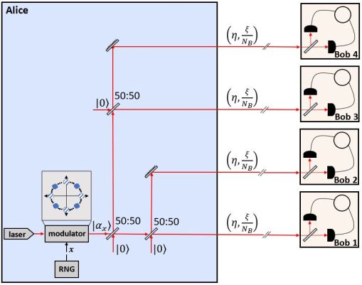
  Figure 1: Sketch of CV-QKD setup with discrete modulation connecting one Alice with multiple Bobs. For ease of presentation, we sketch only four Bobs, albeit our work covers the general case with $N_{B}$ Bobs, which can be easily realized with beamsplitters. In particular, the case for $N_{B}=2^{k}$ can be easily implemented by trees of $50:50$ beamsplitters of depth $k$.

• Error correction— Alice and each of the Bobs communicate over the classical channel to correct their raw keys $\tilde{x}$ and $\tilde{z}^{(i)}$ for $i\in[N_{B}]$.

• Privacy amplification— Finally, the communicating parties perform privacy amplification. Depending on the trust structure, the details of this phase differ slightly.

II.2 QPSK Modulation and Key Map

While the presented arguments apply independently of the chosen discrete modulation scheme and the value of $N_{\mathrm{St}}$, for illustration purposes, we present numerical results for a quadrature phase-shift keying (QPSK) protocol, where Alice prepares $N_{\mathrm{St}}=4$ states (each with probability $1/4$) that are evenly distributed on a circle with radius $|\alpha|$. Then, the key map, which is performed by each of the Bobs in step 4 of the protocol description above, reads as follows, $\forall j\in[N_{B}]:$

$$\tilde{z}_{k}^{(j)}=\left\{\begin{array}[]{ll}0\text{ if }-\frac{\pi}{4}\leq\arg\left(y_{k}^{(j)}\right)<\frac{\pi}{4}&\land~{}\left|y_{k}^{(j)}\right|\geq\Delta_{r},\\ 1\text{ if }\frac{\pi}{4}\leq\arg\left(y_{k}^{(j)}\right)<\frac{3\pi}{4}&\land~{}\left|y_{k}^{(j)}\right|\geq\Delta_{r},\\ 2\text{ if }\frac{3\pi}{4}\leq\arg\left(y_{k}^{(j)}\right)<\frac{5\pi}{4}&\land~{}\left|y_{k}^{(j)}\right|\geq\Delta_{r},\\ 3\text{ if }\frac{5\pi}{4}\leq\arg\left(y_{k}^{(j)}\right)<\frac{7\pi}{4}&\land~{}\left|y_{k}^{(j)}\right|\geq\Delta_{r},\\ \perp\textrm{ otherwise,}\\ \end{array}\right.$$ (1)

where $\arg(y)$ denotes the argument of the complex number $y$, and $\Delta_{r}\geq 0$ is an optional postselection parameter.

III Trust Scenarios

When Alice distributes quantum signals to $N_{B}$ Bobs, several trust scenarios for key generation are possible. In what follows, we consider four different scenarios.

• Alice and one particular Bob trust each other, but distrust all other $N_{B}-1$ Bobs. Alice aims to establish secret keys with the trusted Bob.

• Alice and a group of $1<M_{B}<N_{B}$ Bobs trust each other but distrust all other $N_{B}-M_{B}$ Bobs. Alice aims to establish secret keys with one of the trusted Bobs.

• Alice and all $N_{B}$ Bobs trust each other. Alice aims to establish secret keys with one (trusted) Bob.

• Alice trusts a group of $1\leq M_{B}\leq N_{B}$ Bobs. The $M_{B}$ Bobs are assumed to be legitimate parties, i.e., they do not collaborate with Eve, but also aim for their own private key with Alice, independently of all other Bobs. Alice aims to simultaneously establish secret keys with all trusted Bobs.

Note that a) and c) are special cases of b) for $M_{B}=1$ and $M_{B}=N_{B}$, resp. For ease of notation, without loss of generality, we assume that the first $M_{B}$ Bobs are the trusted ones while the last $N_{B}-M_{B}$ are untrusted. We note that the classical protocol phase in trust-scenario d) fundamentally differs from that in cases a) - c). Here, Alice establishes different secret keys with all the collaborating Bobs, i.e., each of those Bobs sends syndromes $S_{i}$ over the classical channel. However, the syndrome of Bob $i$ can leak information about Bob $j\neq i$, which must be considered in the key rate calculation. One way to avoid this leakage is encrypting the syndromes sent via the classical channel.

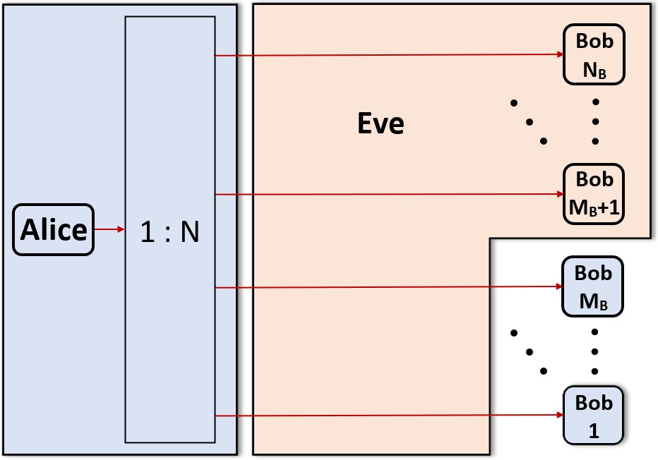
Figure 2: Illustration of different trust scenarios, with a) and c) as special cases of b) for $M_{B}=1$ and $M_{B}=N_{B}$.

IV The Loss-Only Channel

First, we restrict our considerations to the case of the loss-only channel, i.e., we assume that there is no noise. To simplify the presentation, we assume symmetric channels, i.e., the channels connecting Alice with each of the Bobs are all characterized by the same loss parameter $\eta$. However, our method is not restricted to this case and, at the cost of less instructive expressions, accommodates the general, non-symmetric case as well. We generalize the proof method from Ref. [13] to the multi-user case. Note that [13] discusses only a two-state protocol with heterodyne detection; generalizations to protocols with four and higher number of states can be found, for example, in [17, 22, 35]. In the absence of channel noise, it is known that Eve’s optimal attack is the generalized beamsplitter attack, i.e., given that Alice prepared a coherent state $\ket{\alpha_{x}}$, for a channel with loss parameter $\eta$, Bob receives $\ket{\sqrt{\eta}\alpha_{x}}$, while Eve’s share is $\ket{\epsilon_{x}}:=\ket{\sqrt{1-\eta}\alpha_{x}}$. Here, $x\in\left[N_{\mathrm{St}}\right]_{-1}$ labels the state Alice prepared. In what follows, we are always interested in the secure key rate between Alice and one of the Bobs, given certain trust assumptions on the other Bobs as described in the previous section. To simplify our presentation, we assume that the channels connecting Alice with each of the Bobs are identical, i.e., all channels are described by the same loss-parameter $\eta$. However, we want to emphasize that our argument also works for the general case at the cost of more complicated and less instructive expressions. Therefore, due to symmetry, the key rates between Alice and all of the (trusted) Bobs are the same. We denote the Bob with whom Alice aims to establish a secret key with $B_{j}$. Then, the asymptotic secure key rate for cases a) - c) is given by the well-known Devetak-Winter formula [36]:

$$R^{\infty}=\beta I(A:B_{j})-\chi(B_{j}:E),$$ (2)

where $\beta$ is the reconciliation efficiency, $I(A:B_{j})$ denotes the mutual information between Alice and Bob $j$ and $\chi(B_{j}:E)$ is the Holevo information, a quantity bounding Eve’s information about the trusted Bob’s quantum state.

However, for d), where each of the Bobs aims to generate a key with Alice and does not want the other Bobs to hold any information about his key, it is required to take the other Bobs into account. As already discussed in Ref. [31], the Holevo information must be replaced with the maximum of the mutual information held by Eve or any of the other Bobs. Thus, the modified Devetak-Winter formula reads

$$R^{\infty}=\beta I(A:B_{j})-\max\left\{\chi(B_{j}:E),\max_{i\neq j}\{I(B_{j},B_{i})\}\right\}.$$ (3)

In both cases, the main task is to calculate the Holevo quantity, bounding Eve’s information for the given situation, since quantifying the correlation between the Bobs for trust scenario d) does not involve Eve’s system. Therefore, we aim to describe Eve’s system as an orthonormal system.

IV.1 Direct Proof

To illustrate the idea and to point out an issue with a direct analytical approach, let us first focus on scenario c) from the previous section, where Alice trusts all Bobs and aims to establish keys with Bob $i$ and performs the QPSK protocol from Section II.2. Assume Alice prepared $\ket{\alpha_{x}}$ in her lab. She splits the state into $N_{B}$ equal shares and distributes them over $N_{B}$ noiseless channels characterized by a transmittance $\eta$ to all Bobs. The Bob with whom Alice aims to establish keys then obtains $\ket{\sqrt{\frac{\eta}{N_{B}}}\alpha_{x}}$. Eve performs a generalized beamsplitting attack and obtains $\ket{\beta_{x}}:=\ket{\sqrt{\frac{1-\eta}{N_{B}}}\alpha_{x}}$ from each of the channels. The goal is to find a low and finite-dimensional way to represent and diagonalize this state, allowing us to calculate the Holevo quantity.

As we show in Appendix A for a general phase-shift keying protocol, we can express Eve’s state given Alice prepared $\ket{\alpha_{x}}$ as a superposition of basis states $\ket{b_{z}}$,

$$\ket{\Psi_{x}}_{E}=\sum_{z=0}^{3}c_{z}e^{i\arg(\beta_{x})z}\ket{b_{z}}_{E},$$

where the coefficients have the form

$$c_{z}=\sqrt{\sum_{\overset{a_{1},...,a_{N_{B}-1}=0}{\sum_{s}a_{s}=z}}^{3}\prod\limits_{s=1}^{N_{B}}k_{a_{s}}},$$ (4)

with

$$k_{j}:=e^{-|\beta|^{2}}\sum_{s=0}^{\infty}\frac{|\beta|^{2(N_{\mathrm{St}}n_{s}+j)}}{\left(N_{\mathrm{St}}n_{s}+j\right)!}$$

for $j\in\{0,1,2,3\}$. Note that we omitted the subscript $x$ in $\beta_{x}$ because of the symmetry of the considered QPSK protocol. The special form of $|\Psi_{x}\rangle_{E}$ allows an analytic calculation of the Holevo quantity $\chi(B:E)=H(\rho_{E})-\sum_{j=0}^{3}P(Z=j)H(\rho_{E,j})$, where $\rho_{E,j}$ is Eve’s conditional state given that Bob measured the symbol associated with $j$,

$$\rho_{E,j}:=\sum_{x=0}^{3}\frac{P(X=x,Z=j)}{P(Z=j)}\outerproduct{\Psi_{x}}{\Psi_{x}}_{E}$$

and $\rho_{E}:=\sum_{j=0}^{3}P(Z=j)\rho_{E,j}$.

However, as the number of summands in (4) grows exponentially with the number of Bobs involved, i.e., as $4^{N_{B}-1}$. So, even for QPSK with $N_{\mathrm{St}}=4$ the calculation of the coefficients $c_{z}$ becomes already time-consuming (and potentially inaccurate) for double-digit $N_{B}$. Thus, it is evident that one requires a more efficient method for a larger number of Bobs (and/or a larger number of signal states). The same applies to the case where we trust some but not all of the Bobs, which, in principle, can be done similarly, but suffers from the same computational issue.

IV.2 Reduction to Single Bob Case

As the optimal attack in the loss-only scenario is known, this might allow for simplifications or even reductions from the $N_{B}$ Bobs to a $n<N_{B}$ Bob case. For the following argument, we consider the most general scenario b), where Alice distributes quantum signals to $N_{B}$ Bobs where only $M_{B}$ are trusted, while all other $N_{B}-M_{B}$ Bobs are assumed to collaborate with Eve. Since cases a) and c) are special cases thereof, they follow from the general case by setting $M_{B}=1$ and $M_{B}=N_{B}$. We do not restrict our considerations to a specific (discrete) modulation pattern, hence, in general, Alice samples states from an arbitrary discrete set $\{\alpha_{0},...,\alpha_{N_{\mathrm{St}}-1}\}$ according to some discrete distribution. Again, to simplify the argument, we assume that the channels between Alice and each of the Bobs are characterized by the same loss parameter $\eta$. If we set $\eta:=\max_{i}\{\eta_{i}\}$, we obtain valid lower bounds for the key rate in the asymmetric case. However, a tight derivation for the general non-symmetric case can be done along similar lines, leading to less instructive explanations and significantly more complicated expressions.

We start by modeling the channel behavior. Since we assume $M_{B}$ Bobs are trusted, we can attribute the $N_{B}-M_{B}$ untrusted outputs of Alice’s lab directly to Eve. Thus, we replace the $1:N_{B}$ beamsplitter in Alice’s lab by a $\frac{M_{B}}{N_{B}}:\frac{N_{B}-M_{B}}{N_{B}}$ beamsplitter BS 1, where the second output $\ket{\sqrt{1-\frac{M_{B}}{N_{B}}}\alpha_{x}}_{E^{\prime}}$ is directly routed to Eve. The trusted output $\ket{\sqrt{\frac{M_{B}}{N_{B}}}\alpha_{x}}_{B^{\prime}}$ hits another (multi-port) beam-splitter BS 2, dividing the input signal into $M_{B}$ equal shares $\bigotimes_{l=1}^{M_{B}}\ket{\frac{1}{\sqrt{N_{B}}}\alpha_{x}}_{B_{l}^{\prime\prime}}$, one for each trusted Bob. Each of those signals propagates through a separate lossy quantum channel, where according to the general beam splitting attack (with a set of beam splitters, BS 3), Eve obtains each a share $\ket{\sqrt{\frac{1-\eta}{N_{B}}}\alpha_{x}}_{E_{l}}$, while each of the Bobs receives $\ket{\sqrt{\frac{\eta}{N_{B}}}\alpha_{x}}_{B_{l}}$.

The whole procedure can be summarized as,

$$\ket{\alpha_{x}}\stackrel{{\scriptstyle\textrm{BS 1}}}{{\mapsto}}$$

$$\ket{\sqrt{\frac{M_{B}}{N_{B}}}\alpha_{x}}_{A^{\prime}}\otimes\ket{\sqrt{1-\frac{M_{B}}{N_{B}}}\alpha_{x}}_{E^{\prime}}\stackrel{{\scriptstyle\textrm{BS 2}}}{{\mapsto}}$$

$$\bigotimes\limits_{l=1}^{M_{B}}\ket{\frac{1}{\sqrt{N_{B}}}\alpha_{x}}_{A_{l}^{\prime\prime}}\otimes\ket{\sqrt{1-\frac{M_{B}}{N_{B}}}\alpha_{x}}_{E^{\prime}}\stackrel{{\scriptstyle\textrm{BS 3}}}{{\mapsto}}$$

$$\bigotimes\limits_{l=1}^{M_{B}}\left(\ket{\sqrt{\frac{\eta}{N_{B}}}\alpha_{x}}_{B_{l}}\otimes\ket{\sqrt{\frac{1-\eta}{N_{B}}}\alpha_{x}}_{E_{l}}\right)\otimes\ket{\sqrt{1-\frac{M_{B}}{N_{B}}}\alpha_{x}}_{E^{\prime}}.$$

In the following, we make use of two facts: (i) We can efficiently solve the single Bob case in which Eve holds a single coherent state, and (ii) unitary transformations on Eve’s systems leave her Holevo information invariant. Therefore, we try to unitarily combine all separate coherent states that Eve holds into a single coherent state. We use photon number conservation as a shortcut to obtain the magnitude of the single coherent state of Eve and search for a unitary transformation that combines the outputs $E^{\prime}$ and all the $E_{l}$ such that Eve holds $\ket{\sqrt{1-\frac{M_{B}\eta}{N_{B}}}\alpha_{x}}_{E}$ while having the vacuum state in all other systems. In other words, we ask if there exists a linear optics transformation with complex coefficients $a$ and $b_{l}$ for $l\in\left[M_{B}\right]$ such that

$$a\sqrt{1-\frac{M_{B}}{N_{B}}}\alpha_{x}+\sum_{l=1}^{M_{B}}b_{l}\sqrt{\frac{1-\eta}{N_{B}}}\alpha_{x} =\sqrt{1-\frac{M_{B}\eta}{N_{B}}}\alpha_{x}$$

$$|a|^{2}+\sum_{l=1}^{M_{B}}|b_{l}|^{2} =1$$

holds. Due to symmetry we anticipate that $\forall l\in\left[M_{B}\right]:~{}b_{l}=\frac{b}{\sqrt{M_{B}}}$ holds and obtain the solution

$$a =\sqrt{\frac{N_{B}-M_{B}}{N_{B}-M_{B}\eta}},$$

$$b =\sqrt{\frac{M_{B}(1-\eta)}{N_{B}-M_{B}\eta}}.$$

Hence, we could show that Eve can superpose all her coherent states into a single mode $\ket{\Psi_{x}}_{E}=\ket{\sqrt{1-\frac{M_{B}\eta}{N_{B}}}\alpha_{x}}_{E}$ which is in a tensor product with vacuum states only by quantum optical operations (i.e., beam splitters). Thus, we have simplified the general $N_{B}$ user scenario effectively to a single Alice to Bob scenario with a modified Eve term, which allows us to calculate a lower bound on the secure key rate without exponentially growing terms like in the direct approach in Section IV.1. In fact, the computational demands are now independent of the number of users and, therefore, scalable. Note that by setting $M_{B}=1$, we obtain $\ket{\sqrt{1-\frac{\eta}{N_{B}}}\alpha_{x}}_{E}$, which is the result we expect for the particular case of trust-scenario a), and for $M_{B}=N_{B}$, corresponding to trust-scenario c), we obtain $\ket{\sqrt{1-\eta}\alpha}_{E}$, which as well meets expectations for this particular case. The Holevo quantity can then be calculated along the same lines as in the previous section and we yield the same results as with the direct method, but significantly quicker. The mutual information between Alice and Bob $i$ is calculated similarly to the single-user case, always keeping in mind that the key-generating Bob only receives $\ket{\sqrt{\frac{\eta}{N_{B}}}\alpha_{x}}$. A similar consideration allows for calculating the mutual information between Bob $i$ and other Bobs. Then, the asymptotic secure key rate for scenarios a) - d) follows immediately. We present results for key rates in Section VI.

V The Lossy & Noisy Channel

Having dealt with the loss-only case in the previous section, it remains to derive secure key rates for the multi-user scenario for general (i.e., lossy & noisy) channels. The results we obtained for the loss-only case then serve as a benchmark for low noise parameters in the general case and represent upper bounds on those general key rates. We analyze the general case for arbitrary discrete modulation using the numerical security proof method introduced in Refs. [33, 34] and applied in Refs. [17, 19, 24] to DM CV-QKD, focussing on the asymptotic case. In what follows, we briefly explain the idea of the security proof method for the single Bob case and show how it is adapted and applied to the multi-user case. We refer to Refs. [33, 34, 17, 19] for further details.

V.1 Introduction to the Numerical Method Used

We aim to calculate secure key rates for the protocol introduced in Section II, where Bob performs heterodyne detection, described by a POVM $\left\{\outerproduct{\zeta}{\zeta}\right\}_{\zeta\in\mathbb{C}}$, while in the source-replacement [37, 38] picture, Alice’s POVM reads $\{\outerproduct{i}{i}\}_{i=0}^{N_{\mathrm{St}}-1}$.

Applying the dimension reduction method [19], one can rewrite the Devetak-Winter formula as the following optimization problem.

$$R^{\infty}=\min_{\rho\in\mathcal{S}}H\left(Z|E\right)_{\Phi(\rho)}-\delta^{\mathrm{EC}}-\Delta(W),$$ (5)

where $\mathcal{S}$ is a subset of the set of all density operators defined by physical requirements and experimental observations, $\Phi$ is a quantum channel describing the protocol steps, $\delta^{\mathrm{EC}}$ denotes the error-correction leakage, $W\geq\mathrm{Tr}\left[\rho\Pi^{\perp}\right]$ is the so-called weight of the state outside some finite-dimensional cutoff space $\mathcal{H}^{\text{fin}}$ of $\mathcal{H}$ with $\Pi^{\perp}$ being the projection onto the complement of that space, and

$$\Delta(W):=\sqrt{W}\log_{2}(|Z|)+(1+\sqrt{W})h\left(\frac{\sqrt{W}}{1+\sqrt{W}}\right)$$ (6)

is the improved weight-dependent correction term from [39].

Intuitively, the task is to minimize the key rate over all density matrices compatible with the observations. It turns out that this optimization problem can be rewritten as a semi-definite program with a non-linear objective function. The method introduced in Refs. [33, 34] tackles this optimization problem by a two-step process. In the first step, a linearized version of the problem is solved iteratively, using, for example, the Frank-Wolfe algorithm [40]. The output of step 1, which is only an approximate solution to the problem, is then turned into a reliable lower bound in step 2, using SDP duality theory. Additionally, the influence of numerical constraint-violations on the result is taken into account. The gap between step 1 and step 2 can be used to monitor the result’s quality. In almost all cases, the results of step 1 and step 2 (which represent an upper- and lower bound on the secure key rate, respectively) differ only negligibly, indicating tight lower bounds.

This method allows us to consider untrusted ideal and trusted non-ideal detectors, as described in [18]. Following the notation there, we denote the trusted detection efficiency of Bob’s detectors by $\eta_{D}$ and the trusted electronic noise by $\nu_{\mathrm{el}}$. For simplicity, we assume that both homodyne detectors, forming one heterodyne detector, are characterized by the same parameters $(\eta_{D},\nu_{\mathrm{el}})$. Note that this can be easily achieved by choosing $\eta_{D}:=\min(\eta_{D,1},\eta_{D,2})$ and $\nu_{\mathrm{el}}:=\max(\nu_{\mathrm{el},1},\nu_{\mathrm{el},2})$, which leads to slightly pessimistic, but secure lower bounds.

The method and its extensions introduced in the present paper build up upon code from Ref. [24] (which builds up upon code by Ref. [19]) and was implemented in Matlab^® version R2022a. The convex optimization problems are modeled using CVX [41, 42], and we used the MOSEK solver (version 10.0.34) [43] to solve semidefinite programs numerically.

V.2 Generalization to Multiple Bobs

Now, let us generalize this method to the case of multiple Bobs. As untrusted Bobs are assumed to collaborate with Eve, we can immediately reduce the general case to scenario b) by attributing all information that goes to untrusted Bobs directly to Eve. Since in QKD, we conservatively assume that all losses are due to Eve, we can include untrusted Bobs simply by modifying $\eta\mapsto\frac{M_{B}}{N_{B}}\eta$. Without loss of generality, to simplify notation, we assume that the first $M_{B}$ Bobs are trusted. The crucial part for all four scenarios is to quantify Eve’s information about the key. Since scenarios a) and c) are special cases of scenario b), and the expression for Eve’s information about the key in scenario d) is the same as in scenario b) (see Eqs. (2) and (3)), we can discuss the main task for all four cases at once.

We analyze the generalized problem within the postprocessing framework of Refs. [17, 19]. Therefore, let $\mathcal{S}$ denote the set of density matrices compatible with the experimental observations and the requirement that Alice’s reduced density matrix remains unchanged. Let us denote Alice’s, the Bobs’ and Eve’s quantum systems by $A$, $B_{i}$, and $E$, respectively, whereas Eve’s system purifies Alice’s and the Bobs’ joint density matrix, i.e., $\rho_{AB_{1}...B_{M_{B}}E}$ is pure. Furthermore, let $\bar{A}$ and $\bar{B}_{i}$ denote Alice’s and each of the Bobs’ private registers, and let us use tildes to denote their public registers, $\tilde{A}$, $\tilde{B_{i}}$, for $i\in[M_{B}]$. Let be $j$, the index for the key generating Bob. The values stored in the register are drawn from alphabets $S_{a},S_{b},S_{\alpha}$ and $S_{\beta}$, respectively. Finally, let $X$ and $Z$ denote Alice’s and Bob $j$’s key register. Alice’s and the Bobs’ measurements can be described by a measurement channel $\mathcal{M}$,

$$\mathcal{M}^{(j)}\left(\rho_{AB_{1}...B_{M_{B}}E}\right)$$ (7)

$$=\sum_{k,l}\outerproduct{a_{k}}{a_{k}}_{\tilde{A}}\otimes\outerproduct{\alpha_{k}}{\alpha_{k}}_{\bar{A}}\otimes\outerproduct{b_{l}}{b_{l}}_{\tilde{B_{j}}}\otimes\outerproduct{\beta_{l}}{\beta_{l}}_{\bar{B}_{j}}$$

$$~{}~{}~{}\otimes\left[\sqrt{P_{A}^{(k)}}\otimes\sqrt{P_{B_{j}}^{(l)}}\right]\rho_{AB_{T}E}\left[\sqrt{P_{A}^{(k)}}\otimes\sqrt{P_{B_{j}}^{(l)}}\right],$$

where $\left\{P_{B_{j}}^{(l)}\right\}$ denotes Bob $j$’s POVM, and we implicitly assume that on registers we do not mention explicitly, we perform the identity. The action of the key map can be represented by the following isometry

$$V=\sum_{S_{a},S_{b},S_{\beta}}\ket{g(a,b,\beta)}_{Z}\otimes\outerproduct{a}{a}_{\tilde{A}}\otimes\outerproduct{b}{b}_{\tilde{B}_{j}}\otimes\outerproduct{\beta}{\beta}_{\bar{B}_{j}},$$ (8)

where the $g:S_{a}\times S_{b}\times S_{\beta}\rightarrow\{0,...,N_{\text{St}},\perp\}$ is the key map function and $\perp$ is the symbol we use to denote discarded signals. Then, the final classical-quantum state between the key register and Eve reads

$$\tilde{\rho}_{Z[E]} =V\text{Tr}_{A\bar{A}B_{1}...B_{j-1}B_{j}\bar{B}_{j}B_{j+1}...B_{M_{B}}}\left[\mathcal{M}\left(\rho_{AB_{T}E}\right)\right]V^{\dagger}$$ (9)

$$=\text{Tr}_{A\bar{A}B_{1}...B_{j-1}B_{j}\bar{B}_{j}B_{j+1}...B_{M_{B}}}\left[V\mathcal{M}\left(\rho_{AB_{T}E}\right)V^{\dagger}\right]$$

$$= :\Phi\left(\rho_{AB_{1}...B_{M_{B}}E}\right).$$

The starting point for our examination in scenario b) is the Devetak-Winter formula, which can be rewritten as

$$R^{\infty} =I(X:Z)-I(Z:E)=H(Z|E)-H(Z|X),$$

where the occurring quantities are evaluated on the state processed by the communicating parties. Here, $Z$ and $X$ denote Bob $j$’s and Alice’s key string. Since we aim for a lower bound on the secure key rate, we have to minimize this expression over all states compatible with all (trusted) Bobs’ observations. We replace the second term with the actual error correction leakage $\delta_{EC}^{\text{leak}}$ and thus are only left with an optimization over the first term. We obtain

$$R^{\infty}=\min_{\mathcal{S}}H(Z|E)_{\tilde{\rho}_{ZE}}-\delta_{EC}^{\text{leak}}.$$ (10)

For scenario d), along similar lines, we can rewrite the key rate formula from Eq. (3) as

$$R^{\infty}=\min\left\{\min_{\mathcal{S}}H(Z|E)_{\tilde{\rho}_{ZE}},\min_{i}\{H(Z|B_{i})\}\right\}-\delta_{EC}^{\text{leak}}.$$ (11)

Our main task in what follows is to determine $\min_{\mathcal{S}}H(Z|E)_{\tilde{\rho}_{ZE}}$, which is the same for both cases. Following the ideas in [44], we can simplify $H(Z|E)_{\tilde{\rho}_{ZE}}$ further. To simplify notation, we extend the short notation $B_{T}$ for $B_{1}...B_{M_{B}}$ to $B_{T\setminus j}$ in case we mean $B_{1},...,B_{j-1},B_{j+1},...,B_{M_{B}}$, i.e., to denote all Bobs’ registers but $B_{j}$. Then, note that $\tilde{\rho}_{AB_{T}}=\sum_{i}Z_{i}\rho_{AB_{T}}Z_{i}$ for $Z_{i}$ being orthogonal projectors with $\sum_{i}Z_{i}=\mathbbm{1}$, which allows us to rewrite the term we want to minimize

$$H(Z|E)_{\tilde{\rho}_{ZE}}$$

$$= H(\tilde{\rho}_{ZE})-H(\rho_{E})$$

$$= H(\tilde{\rho}_{AB_{T}})-H(\rho_{AB_{T}})$$

$$= -\mathrm{Tr}\left[\tilde{\rho}_{AB_{T}}\log_{2}\tilde{\rho}_{AB_{T}}\right]-H(\rho_{AB_{T}})$$

$$= \mathrm{Tr}\left[-\rho_{AB_{T}}\log_{2}\tilde{\rho}_{AB_{T}}+\rho_{AB_{T}}\log_{2}\rho_{AB_{T}}\right]$$

$$= D\left(\rho_{AB_{T}}\right|\!\left|\tilde{\rho}_{AB_{T}}\right).$$

The first equality is the definition of the conditional entropy; for the second equality, we use that $\rho_{AB_{T}E}$ is pure, and the fourth equality exploits the fact that $\tilde{\rho}_{AB_{T}}$ is already block-diagonal, hence we can replace the first $\tilde{\rho}_{AB_{T}}$ by $\rho_{AB_{T}}$ without changing the result. Finally, for the last equality, we use the definition of the quantum relative entropy. A more detailed argument follows the lines of [17, Appendix A]. This justifies using the numerical method from Refs. [33, 34], tailored for the quantum relative entropy.

Next, let us discuss the optimization problem for the objective protocol in detail. Recall that Alice prepares one out of $N_{\textrm{St}}$ quantum states and sends them to the Bobs, who are equipped with heterodyne detectors. In every testing round, one of the Bobs measures to determine the expected value of certain observables (in our case $\hat{n}_{\beta_{i}}$ and $\hat{n}_{\beta_{i}}^{2}$ as we will discuss later). In key-generation rounds, all but one Bob act passively, while the key-generating Bob’s POVM is $\left\{\frac{1}{\pi}\outerproduct{\zeta}{\zeta}\right\}_{\zeta\in\mathbb{C}}$. Finally, in the source-replacement picture [37, 38], Alice’s POVM is given by $\left\{\outerproduct{i}{i}\right\}_{i=0}^{N_{\text{St}}-1}$. For key generation, we perform a key map that assigns measurement outcomes lying in a certain region of phase space some logical bit-value. Therefore, we need to combine the POVM elements corresponding to a certain region to obtain the corresponding coarse-grained POVM (see also Ref. [17])

$$R_{B_{j}}^{z}=\frac{1}{\pi}\int_{A_{z}}\outerproduct{\zeta}{\zeta}d^{2}\zeta,$$ (12)

where $A_{z}$ labels the region. For the objective QPSK protocol, $z\in\{0,1,2,3\}$ and $A_{z}$ are wedges in phase space, defined in Eq. (1). As outlined in [19], the key map for our protocol simply copies Bob’s private register $\bar{B}$ to $Z$, hence we can relabel $\bar{B}$ to $Z$. Thus, we finally obtain for the postprocessing map $\Phi$, defined in Eq. (9)

$$\Phi\left(\rho_{AB_{T}E}\right)=$$ (13)

$$~{}\sum_{z=0}^{N_{\text{St}}-1}\ket{z}_{Z}\otimes\text{Tr}_{AB_{T}}\left[\rho_{AB_{T}E}\left(R_{B_{j}}^{z}\ast\mathbbm{1}_{AB_{T\setminus j}}\right)\right],$$

where we introduced the notation $\hat{O}_{B_{j}}\ast\mathbbm{1}_{AB_{T\setminus j}}:=\mathbbm{1}_{AB_{1,...,j-1}}\otimes\hat{O}_{B_{j}}\otimes\mathbbm{1}_{AB_{j+1,...,M_{B}}}$ for the operator $\hat{O}$ acting on the $j$-th Bob system and identity operators acting on Alice’ and all other Bobs’ systems. Furthermore, according to Ref. [17, Appendix A], we omitted redundant registers.

Similar to the single-Bob case [19], the expected coherent state Bob receives in the case of a loss-only channel is $\ket{\beta_{i}}=\hat{D}(\beta_{i})\ket{0}$, where $\beta_{i}:=\sqrt{\eta}\alpha_{i}$ and $\{\beta_{i}\}_{i=0}^{N_{\text{St}}-1}$ is a set of complex numbers that we use to parametrize basis vectors and observables later on. However, considering lossy & noisy channels, we expect Bob to receive a displaced thermal state. This motivates the basis of displaced number states $\ket{n_{\beta_{i}}}=\hat{D}(\beta_{i})\ket{n}$ as an efficient choice for a basis for our finite-dimensional subspace. This choice will allow us to describe the received state sufficiently well with a small number of basis states (as in the limit of no noise, only one vector suffices). Since this applies to each Bob, we naturally generalize the choice for the single-Bob case to the multi-Bob case and choose the following projection

$$\Pi^{N_{c}}_{\beta_{i},M_{B}}:=\bigotimes_{k=1}^{M_{B}}\sum_{n=0}^{N_{c}}\outerproduct{n_{\beta_{i}}}{n_{\beta_{i}}}.$$ (14)

This already sets the stage for the generalization of observables used in [19] to the multi-Bob case, as it will turn out to be beneficial if they commute with the projection onto the finite-dimensional state we just chose. We choose the observables to be $\hat{n}_{\beta_{i}}:=\hat{D}(\beta_{i})\hat{n}\hat{D}^{\dagger}(\beta_{i})$ and $\hat{n}^{2}_{\beta_{i}}:=\hat{D}(\beta_{i})\hat{n}^{2}\hat{D}^{\dagger}(\beta_{i})$ which are easily accessible by heterodnye measurement (for details see [39]). Then, the set of observables for our protocol read

$$\left\{\hat{\Gamma}_{i,k},\hat{\Gamma}^{\text{sq}}_{i,k}\right\}_{i\in\left[N_{\text{St}}\right]_{-1}}^{k\in\left[M_{B}\right]}.$$ (15)

with

$$\hat{\Gamma}_{i,k} :=\outerproduct{i}{i}_{A}\otimes\left[\left(\hat{n}_{\beta_{i}}\right)_{B_{k}}\ast\mathbbm{1}_{B_{T\setminus k}}\right],$$ (16)

$$\hat{\Gamma}^{\text{sq}}_{i,k} :=\outerproduct{i}{i}_{A}\otimes\left[\left(\hat{n}^{2}_{\beta_{i}}\right)_{B_{k}}\ast\mathbbm{1}_{B_{T\setminus k}}\right].$$

Note, that they commute with $\Pi^{N_{c}}_{\beta_{i},M_{B}}$ from Eq. (14).

It remains to determine the weight outside of the cutoff space defined by $\Pi^{N_{c}}_{\beta_{i},M_{B}}$, where $\overline{\Pi^{N_{c}}_{\beta_{i},M_{B}}}:=\mathbbm{1}-\Pi^{N_{c}}_{\beta_{i},M_{B}}$. The generalized version of the dual SDP for $W_{i}=\mathrm{Tr}\left[\rho_{B_{T}}\overline{\Pi^{N_{c}}_{\beta_{i},M_{B}}}\right]$ given in the proof of Theorem 5 in Ref.[19] reads

$$\min_{\vec{y}}y_{0}+\sum_{k=1}^{M_{B}}y_{k}\langle\hat{\Gamma}_{i,k}\rangle+y_{k}^{\text{sq}}\langle\hat{\Gamma}^{\text{sq}}_{i,k}\rangle$$

s.t.:

$$~{}y_{0}\mathbbm{1}_{B_{T}}+\sum_{k=1}^{M_{B}}y_{k}\hat{\Gamma}_{i,k}+y_{k}^{\text{sq}}\hat{\Gamma}^{\text{sq}}_{i,k}-\overline{\Pi^{N_{c}}_{\beta_{i},M_{B}}}\geq 0$$

$$~{}\vec{y}\in\mathbb{R}^{2M_{B}+1}.$$

The positivity of the operator on the RHS of the first constraint is equivalent to all eigenvalues of this operator being non-negative. Taking into account the structure of this operator, we observe that $\forall k\in\{1,...,M_{B}\}:~{}y_{k}+y_{k}^{\text{sq}}\geq 0$ which implies $y_{k}\geq-y_{k}^{\text{sq}}$. Additionally, we identify the following candidates for the smallest eigenvalue

$$\lambda(m_{1},...,m_{M_{B}-1})=y_{0}-1+\sum_{k=1}^{M_{B}}m_{k}y_{k}+m_{k}^{2}y_{k}^{\text{sq}},$$

where $m_{1},...,m_{M_{B}}\in\{0,...,N_{c}+1\}$, with $m_{1}=...=m_{B}=N_{c}+1$ being the worst-case candidate. It follows readily that $y_{k}=-\frac{1}{M_{B}N_{C}(N_{C}+1)}$ and $y_{k}^{\text{sq}}=\frac{1}{M_{B}N_{C}(N_{C}+1)}$ together with $y_{0}=0$ solves all conditions on the eigenvalues simultaneously. Noting that $\left\langle\left(\hat{n}_{\beta_{i}}\right)_{B_{k}}\ast\mathbbm{1}_{B_{T\setminus k}}\right\rangle=\langle\hat{n}_{\beta_{i}}\rangle$ and $\left\langle\left(\hat{n}^{2}_{\beta_{i}}\right)_{B_{k}}\ast\mathbbm{1}_{B_{T\setminus k}}\right\rangle=\langle\hat{n}^{2}_{\beta_{i}}\rangle$ we obtain

$$W_{i}=\frac{\langle\hat{n}^{2}_{\beta_{i}}\rangle-\langle\hat{n}_{\beta_{i}}\rangle}{N_{c}(N_{c}+1)},$$ (17)

which coincides with the single Bob case. Thus, we obtain for the weight, in accordance with the single Bob case from Ref. [19],

$$W=\sum_{i=0}^{N_{\textrm{St}}-1}p_{i}\frac{\langle\hat{n}^{2}_{\beta_{i}}\rangle-\langle\hat{n}_{\beta_{i}}\rangle}{N_{c}(N_{c}+1)}.$$ (18)

Having discussed and specified all parts that differ from the single Bob case, we finally can formulate the relevant optimization problem, in analogy to the single Bob case in Ref. [19], but using the improved correction from Ref. [39]. We define the objective function

$$f(\rho):=H(Z|E)_{\Phi(\rho)}$$ (19)

and arrive at the following minimization problem

$$\text{min}_{\rho} f(\rho)$$ (20)

s.t.:

$$1-W\leq\mathrm{Tr}\left[\rho\right]\leq 1,$$

$$\frac{1}{2}\left|\left|\text{Tr}_{B_{T}}\left[\rho\right]-\rho_{A}\right|\right|_{1}\leq\sqrt{W},$$

$$\mathrm{Tr}\left[\rho\frac{1}{p_{i}}\hat{\Gamma}_{i,k}\right]\leq\gamma_{i,k},$$

$$\mathrm{Tr}\left[\rho\frac{1}{p_{i}}\hat{\Gamma}_{i,k}^{\text{sq}}\right]\leq\gamma_{i,k}^{\text{sq}},$$

$$\rho\geq 0,$$

where $\rho_{A}=\sum_{m,n=0}^{N_{\text{St}}-1}\sqrt{p_{m}p_{n}}\bra{\alpha_{n}}\ket{\alpha_{m}}\ket{m}\!\!\bra{n}$, the $\hat{\Gamma}_{i,k}$ and $\hat{\Gamma}_{i,k}^{\text{sq}}$ have been defined in Eq. (16) and $\gamma_{i,k}:=\langle\hat{\Gamma}_{i,k}\rangle=\langle\hat{n}_{\beta_{i}}\rangle$, $\gamma_{i,k}^{\text{sq}}:=\langle\hat{\Gamma}_{i,k}^{\text{sq}}\rangle=\langle\hat{n}^{2}_{\beta_{i}}\rangle$ for $i\in\left[N_{\text{St}}\right]_{-1},k\in\left[M_{B}\right]$ This optimization problem can be solved using the numerical two-step algorithm from Refs. [44, 34]. Denoting the found optimum by $\rho^{*}$, we finally obtain for the key rate

$$R^{\infty}=f(\rho^{*})-\delta_{EC}^{\text{leak}}-\Delta(W),$$ (21)

where $\Delta(W)$ is the improved correction term given in Eq. (6).

To consider imperfect detectors and/or trusted detection noise, the POVM for the ideal heterodyne measurement must be replaced with the POVM of the non-ideal heterodyne measurement which affects the region-operators in the objective function and the observables in the constraints, as explained in [18].

VI Results

We illustrate our findings for the quadrature phase-shift keying (QPSK) protocol (see Section II.2). However, we emphasize that this is just a choice for illustration purposes since our findings in the previous sections are general. Furthermore, to ease presentation, we consider the symmetric case. This means the channels connecting Alice with each of the Bobs are all characterized by the same loss parameter $\eta$ and, in case of noisy channels, the excess-noise $\xi$ is distributed evenly among all channels. The labs of each of the Bobs are equipped with detectors with the same detection-efficiency $\eta_{D}$ and electronic noise $\nu_{\mathrm{el}}$. This assumption, however, is only made to ease presentation and is not necessary for our method.

In the following, we assume standard optical fibers with $0.2$dB loss per kilometer in our loss model. We consider the case where Alice and Bob perform reverse reconciliation, in which Alice corrects her errors according to the information she receives from Bob via the classical channel. We assume a constant reconciliation efficiency of $\beta=95\%$ to allow comparability with existing works on single-user QKD. However, we want to note that achieving a continuous error-correction efficiency over a wide range of transmissivities, hence for different orders of signal-to-noise ratio, is challenging. To date, it is unclear if this can be achieved with current error-correction routines. We refer the reader to Ref. [45] for an in-depth discussion. We start our conversation with the loss-only case, followed by the general case of lossy & noisy channels.

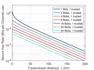
(a) Scenario a), i.e., all other Bobs untrusted

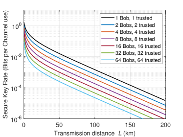
(b) Scenario c), i.e., all Bobs trusted

Figure 3: QPSK key rate for a single Bob vs transmission distance for the loss-only channel.

VI.1 Key Rates for the Loss-Only Channel

In Section IV, we have presented two equivalent methods for calculating asymptotic secure key rates for the loss-only case. However, since the second method, introduced in Section IV.2, where we reduced the multi-Bob scenario to the single-Bob case, is significantly faster, and both the problem size and calculation times are independent of the number of Bobs, we will focus on this method, allowing us to analyze settings with an arbitrary number of Bobs. For each fixed distance, we optimized the secure key rate over the coherent state amplitude $\alpha$ in the interval $[0.3,5]$ using the built-in Matlab® routine fminbnd applied to the negative objective function.

Having clarified the parameters and the method used, let us discuss our results for different trust scenarios (see Section III). In Figure 3a, we present asymptotic secure key rates for Scenario a), where Alice and the key-generating Bob distrust all other Bobs, i.e., assume all other Bobs collaborate with Eve. We illustrate this case for $2^{n}$ Bobs, where $n\in\{0,1,2,3,4,5,6\}$. However, this is just for illustration purposes, as our method allows an arbitrarily high number of Bobs, also beyond powers of $2$. Note that the $1$ Bob curve corresponds to the single-user case, already known from earlier works [17, 22].

In Figure 3b, we present asymptotic secure key rates for Scenario c), where Alice and the key-generating Bob trust all other Bobs. Again, the $1$ Bob curve corresponds to the case already known from single-user DM CV-QKD. We observe qualitatively similar behavior for large transmission distances and a significant increase in key rate compared to the fully untrusted case for low transmission distances. This is aligned with our expectations, based on the reduction found in Section IV.2. While for a fixed total number of Bobs in both cases, the key-generating Bob receives the same signal, the share caught by Eve differs notably. This share can be quantified by $r(\eta):=\sqrt{\frac{1-\eta}{1-\frac{1}{N_{B}}\eta}}$. Inserting $\eta_{1}=0.954$, which corresponds to a distance of $1$km and $\eta_{100}=0.01$, corresponding to a distance of $100$km and, exemplarily, $N_{B}=16$ leads to $r(\eta_{1})=0.219$ and $r(\eta_{100})=0.995$, i.e., for $100$km transmission distance, the signals Eve obtains do hardly differ in both scenarios, while they differ by a factor of about $5$ for $1$km, which explains the observed behavior.

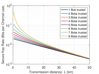
Figure 4: QPSK key rate vs transmission distance for the loss-only channel and eight Bobs. Scenario b), i.e., some Bobs are trusted by Alice.

Finally, in Figure 4, we fix the total number of Bobs to $N_{B}=8$ and (from bottom to top) trust between $1$ and $8$ Bobs. The curves where we do not trust all other Bobs ($1$ Bob trusted) are equivalent to the corresponding curves in Figures 3b and 3a. Again, we observe very different behaviors for low transmission distances, while the obtained key rate curves are qualitatively the same for medium to large distances.

These observations already highlight that trusting some or even all Bobs helps to increase the key rate only for low to medium transmission distances. This, however, is well aligned with the main use case of CV-QKD, which distributes secure quantum keys at a high rate in urban areas and campus networks. In particular, trusting some or even all the Bobs can be a practical and realistic use case for campus networks. However, while in such use cases, it might be reasonable to trust some or even all other Bobs not to collaborate with Eve, the Bobs nevertheless might aim for a private key concerning Eve and all other Bobs. We call this scenario, aligning with trust-scenario d). We illustrate this case for $N_{B}=2,4,6$ and $16$ Bobs in Figure 5, where we optimized $\alpha$ in the interval $[0.3,10]$. We also note that the optimal $\alpha$ for scenario d) differs slightly for low distances. The solid lines correspond to the fully trusted case, while the dotted lines represent the secure key rates in scenario d). We want to highlight that both the solid and the dotted line correspond to the key rate per Bob. While this is equivalent to the total key rate generated by Alice for the trusted case (solid lines), where only one of the Bob generates a key, this differs by a factor of $M_{B}=N_{B}$ from the total key rate generated by Alice in scenario d) (dotted lines). This is because, in the latter case, each of the Bobs’ keys is completely decoupled from all the other Bobs and, therefore, can be used independently by Alice. Considering the key rate per Bob, we observe a noticeable difference in key rate only for very low transmission distances (i.e., in the low-loss case); this small gap even shrinks further for increasing numbers of Bobs. For $N_{B}>=32$, no discernible difference can be observed through visual inspection; thus, we omitted the corresponding curves. This highlights that obtaining keys according to scenario d) w.r.t. the other Bobs comes at only a tiny cost in key rate per Bob, while it significantly increases the key rate generated by Alice. However, in this picture, we have neglected one effect. Namely, the error-correction phase for scenario d) differs from those in the other scenarios since the syndrome transmitted by one Bob might leak information to the other Bobs. One way to avoid this is by encrypting the syndrome. While in the ideal case, where all routines work without errors, this does not come with additional cost since the key is the same length as the syndrome, whose size is subtracted in the key rate formula anyway. If the error correction fails, this procedure uses up the key, thus decreasing the effective key rate. However, since in the asymptotic setting, all subroutines are assumed to work perfectly, we do not consider this error-dependent effect. According to Ref. [31], parts of the lost key can be regained by a recycling procedure that uses the fact that the key used in aborted rounds is ‘hidden’ by the partially random syndrome. While we do not discuss this method in further detail here, we note that it is, in principle, compatible with our work and refer to Ref. [31] for further details.

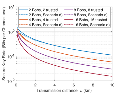
Figure 5: QPSK key rate vs transmission distance for the loss-only channel and scenario d), and the trusted scenario c).

VI.2 Key Rates for the Lossy & Noisy Channel

While the assumption of the loss-only channel helped to simplify the security analysis and allowed for analytical solutions, fast evaluations, and qualitative statements, it is far from reality. Thus, we require a security argument for the general lossy & noisy case. However, the results from the previous section will serve as a helpful benchmark and upper bound for the results in the present section.

Therefore, we apply the security argument presented in Section V.2, using the numerical two-step method by Refs. [33, 34], to obtain secure key rates. While our arguments in Section V.2 apply to a general number of Bobs, calculating secure key rates in this formulation includes solving semi-definite programs. Therefore, computational constraints and limitations need to be taken into account. Let us denote by $n_{c}$ the largest (displaced) Fock state included in the basis of our finite-dimensional cutoff space. Then the numerical dimension of the problem scales as $\mathcal{O}(N_{\textrm{St}}(n_{c}+1)^{M_{B}})$. Thus, it is obvious that to keep the problem numerically feasible, we need to choose a significantly smaller cutoff dimension than for the single Bob case. We found $n_{c}=7$ (thus $\textrm{dim}(\mathcal{H}^{\textrm{fin}})=8$) being a reasonable compromise. Using the dimension reduction method leads to a higher weight $W$, hence a larger correction term $\Delta(W)$, but after all, still valid lower bounds on the secure key rate. Furthermore, with our current computational resources, we had to restrict our numerical evaluations to a maximum of two trusted Bobs, $M_{B}=2$, while keeping the total number of Bobs in principle arbitrary. This is not a fundamental limitation but mainly comes from very RAM-demanding SDP solvers. We expect the number of feasible Bobs can be increased by an improved implementation, using different solvers, better hardware, and/or improved problem formulations that exploit symmetries. Generally, calculating secure key rates for QKD protocols involving high-dimensional systems is known to be RAM-demanding and computationally challenging [46]. However, since this work aims to demonstrate our method, arbitrary $N_{B}$ and fixing $M_{B}=2$ is sufficient for our purposes. We demonstrate the soundness of our implementation in Appendix B and proceed with our results for an excess noise of $\xi=10^{-2}$ (assumed as preparation noise, inserted into the system from Alice’s source). For our plots, for fixed transmission distance $L$, we optimize over the coherent state amplitude $\alpha$ via fine-grained search in steps of $\Delta\alpha=0.01$. Our security argument for the lossy and noisy case was general and applied to an arbitrary number of Bobs. We implemented our numerical algorithm in Matlab R2022b, used CVX [41, 42] to model the SDPs and employed the SDP solver Mosek [43].

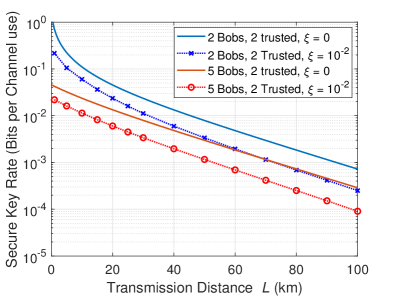
Figure 6: QPSK key rate vs transmission distance for the lossy & noisy channel with $\xi=10^{-2}$. Solid lines are reference curves for the loss-only channel.

In Figure 6, we show the secure key rate for a fixed noise parameter of $\xi=0.01$ as a function of the transmission distance. As discussed in the previous paragraph, we fix the number of trusted Bobs to $M_{B}=2$ and examine a total number of Bobs of $N_{B}=2$ (blue curves) and $N_{B}=5$ (red curves), although there is no fundamental limit on $N_{B}$. For comparison, we also plot the corresponding curves for the loss-only scenario ($\xi=0$) in solid lines. As expected, we observe lowered key rates due to the additional excess noise, but qualitatively similar behavior with loss/transmission distance as for the loss-only case.

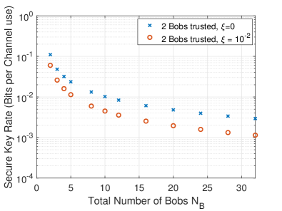
Figure 7: QPSK key rate vs total number of Bobs while two Bobs trust each other ($M_{B}=2$ in Scenario b)) for the lossy & noisy channel with $\xi=10^{-2}$ and $L=10$km.

Finally, we examine the secure key rate of a star network as a function of the number of users in the network (while still trusting $M_{B}=2$ Bobs). For Figure 7, we fixed the transmission distance between Alice and each of the Bobs to $L=10$ km, representing a realistic value for local area and campus networks and plot the secure key rate vs the total number of Bobs, $N_{B}$, both for the loss-only case ($\xi=0$, blue dots) and for $\xi=10^{-2}$ (orange dots). Even in the presence of noise, our network can tolerate $N_{B}=32$ Bobs and beyond in the asymptotic scenario. This demonstrates the feasibility of local-area networks using discrete-modulated continuous-variable quantum key distribution systems.

VII Conclusion

In this study, we introduce a natural extension of continuous-variable quantum key distribution (QKD) with discrete modulation, commonly used in standard point-to-point QKD, to a multi-user setting where a single Alice is connected to multiple Bobs, establishing keys with some or even all of them simultaneously. This represents a significant advancement toward achieving secure communication in complex network environments.

We present a method to calculate achievable secure key rates, considering both loss-only and lossy+noisy channels. Additionally, we explore various trust scenarios and analyze the impact of different trust levels on the secure key rate. Our investigation demonstrates that secure key rates can be achieved for distances and channel attenuations relevant to urban area networks and campus networks. In one scenario, our model shows that the proposed scheme can accommodate a double-digit number of users at urban-area distances (approximately 10 km) and a mid-single-digit number of users in metropolitan area networks (greater than 10 km). The generated keys can directly encrypt messages exchanged between Alice and one or multiple Bobs. Moreover, the mutually generated keys between Alice and each Bob can be used to distribute a random bit string for conference key agreement. This highlights the suitability of discrete modulation continuous-variable QKD for deployment in quantum optical networks, facilitating secure communication among multiple users over near- and mid-range distances, such as those encountered in urban areas and campuses.

While real-world key rates depend on various factors, including implementation details, noise levels, and error-correction efficiency — factors that we could only consider within theoretical models — our study nevertheless demonstrates the feasibility and practicality of multi-user quantum key distribution systems based on discrete-modulated continuous variables.

In this work, we have focussed on key rates in the asymptotic limit. Since the single-Bob case has been proven secure against collective i.i.d. attacks in the finite-size regime in previous studies [23, 47, 24], the obvious next step is to extend our results to scenarios with finitely many exchanged signals.

Appendix A Details for the Direct Loss-Only Proof

In this section, we discuss the mathematical details of the direct proof for the loss-only scenario and general phase-shift keying (PSK) modulation in more detail. The idea is to expand the state in Fock representation and group those Fock states in congruence classes $\textrm{ mod }N_{\mathrm{St}}$. We then define $N_{\mathrm{St}}$ basis vectors. As we want the number of basis vectors to be independent of the number of Bobs, we group them in a special way that ensures mutual orthogonality. So, we first aim to write the state Eve branched off in a different way that allows us to regroup the expressions in an advantageous way.

$$\ket{\Psi_{x}}_{E} =\bigotimes_{b=1}^{N_{B}}\ket{\beta_{x}}_{E_{b}}=e^{-N_{B}\frac{|\beta_{x}|^{2}}{2}}\bigotimes_{b=1}^{N_{B}}\sum_{n_{b}=0}^{\infty}\frac{\beta_{x}^{n_{b}}}{\sqrt{n_{b}!}}\ket{n_{b}}_{E_{b}}$$

$$=e^{-N_{B}\frac{|\beta_{x}|^{2}}{2}}\sum_{n_{1},...,n_{N_{B}}=0}^{\infty}\bigotimes_{b=1}^{N_{B}}\frac{\beta_{x}^{n_{b}}}{\sqrt{n_{b}!}}\ket{n_{b}}_{E_{b}}$$

$$=e^{-N_{B}\frac{|\beta_{x}|^{2}}{2}}\sum_{a_{1},...,a_{N_{B}}=0}^{N_{\mathrm{St}}-1}\sum_{n_{1},...,n_{N_{B}}=0}^{\infty}\bigotimes\limits_{b=1}^{N_{B}}\left(\frac{\beta_{x}^{N_{\mathrm{St}}n_{b}+a_{b}}}{\sqrt{\left(N_{\mathrm{St}}n_{b}+a_{b}\right)!}}\ket{N_{\mathrm{St}}n_{b}+a_{b}}_{E_{b}}\right)$$

$$=e^{-N_{B}\frac{|\beta_{x}|^{2}}{2}}\sum_{z=0}^{N_{\mathrm{St}}-1}\sum_{\overset{a_{1},...,a_{N_{B}}=0}{\sum_{j}a_{j}=z\text{ mod }N_{\mathrm{St}}}}^{N_{\textrm{St}}-1}\sum_{n_{1},...,n_{N_{B}}=0}^{\infty}\bigotimes\limits_{b=1}^{N_{B}}\left(\frac{\beta_{x}^{N_{\mathrm{St}}n_{b}+a_{b}}}{\sqrt{\left(N_{\mathrm{St}}n_{b}+a_{b}\right)!}}\ket{N_{\mathrm{St}}n_{b}+a_{b}}_{E_{b}}\right)$$

In the third line we introduce the said congruence classes $0,1,...,N_{\mathrm{St}}-1$ in each of the systems, and in the last line, we split this sum into $N_{\mathrm{St}}$ parts satisfying $\sum_{j}a_{j}=z\text{ mod }N_{\mathrm{St}}$ for $z\in\left[N_{\mathrm{St}}\right]_{-1}$. This allows us to define

$$\ket{\tilde{b}_{z}^{(x)}}_{E}:=e^{-N_{B}\frac{|\beta_{x}|^{2}}{2}}\sum_{\overset{a_{1},...,a_{N_{B}}=0}{\sum_{j}a_{j}=z\text{ mod }N_{\mathrm{St}}}}^{N_{\textrm{St}}-1}\sum_{n_{1},...,n_{N_{B}}=0}^{\infty}\bigotimes\limits_{b=1}^{N_{B}}\left(\frac{\beta_{x}^{N_{\mathrm{St}}n_{b}+a_{b}}}{\sqrt{\left(N_{\mathrm{St}}n_{b}+a_{b}\right)!}}\ket{N_{\mathrm{St}}n_{b}+a_{b}}_{E_{b}}\right).$$

Note that $\beta_{x}^{N_{\mathrm{St}}n_{b}+a_{b}}=\left|\beta_{x}\right|^{N_{\mathrm{St}}n_{b}+a_{b}}e^{i\arg(\beta_{x})\left(N_{\mathrm{St}}n_{b}+a_{b}\right)}$. Given the symmetry of PSK protocols where $\arg(\alpha_{x})=\frac{2\pi}{N_{\text{St}}}x$, $e^{i\arg(\beta_{x})\left(N_{\mathrm{St}}n_{b}\right)}=1$, which allows us to rewrite the expression as

$$\ket{\tilde{b}_{z}^{(x)}}_{E}:=e^{-N_{B}\frac{|\beta|^{2}}{2}}e^{i\arg(\beta_{x})z}\sum_{\overset{a_{1},...,a_{N_{B}}=0}{\sum_{j}a_{j}=z\text{ mod }N_{\mathrm{St}}}}^{N_{\textrm{St}}-1}\sum_{n_{1},...,n_{N_{B}}=0}^{\infty}\bigotimes\limits_{b=1}^{N_{B}}\left(\frac{\left|\beta\right|^{N_{\mathrm{St}}n_{b}+a_{b}}}{\sqrt{\left(N_{\mathrm{St}}n_{b}+a_{b}\right)!}}\ket{N_{\mathrm{St}}n_{b}+a_{b}}_{E_{b}}\right),$$

which shows that $x$ only occurs in the exponential pre-factor. Next, we normalize those vectors. Let us denote

$$k_{j}:=e^{-|\beta|^{2}}\sum_{s=0}^{\infty}\frac{\left(|\beta|^{2}\right)^{N_{\mathrm{St}}n_{s}+j}}{\left(N_{\mathrm{St}}n_{s}+j\right)!}$$

for $j\in\left[N_{\mathrm{St}}\right]_{-1}$. Note that due to symmetry implied by phase-shift keying modulation, for all $x$, $k_{j}$ is independent of $x$. Consequently, to ease notation, we omitted the descriptor $x$. Then the normalization constant $c_{z}$ for $\ket{\tilde{b}_{z}^{(x)}}_{E}$, which is independent of $x$, reads

$$c_{z}=\sqrt{\innerproduct{\tilde{b}_{z}^{(x)}}{\tilde{b}_{z}^{(x)}}}=\sqrt{\sum_{\overset{a_{1},...,a_{N_{B}-1}=0}{\sum_{s}a_{s}=z}}^{N_{\mathrm{St}}-1}\prod\limits_{s=1}^{N_{B}}k_{a_{s}}},$$ (22)

and the normalized system is given by

$$\ket{b_{z}^{(x)}}_{E}:=\frac{1}{c_{z}}\ket{\tilde{b}_{z}^{(x)}}_{E},$$

for $z\in\left[N_{\text{St}}\right]_{-1}$.

This allows us to express Eve’s state given Alice prepared $\ket{\alpha_{x}}$ in a particularly simple form

$$\ket{\Psi_{x}}_{E}=\sum_{z=0}^{N_{\mathrm{St}}-1}c_{z}e^{i\arg(\beta_{x})z}\ket{b_{z}}_{E},$$

where we pulled out the $x$-dependent exponential factor from $\ket{b_{z}^{(x)}}_{E}$, defining $\ket{b_{z}}_{E}:=e^{-i\arg(\beta_{x})z}\ket{b_{z}^{(x)}}_{E}$. Next, we notice the following

Lemma 1.

For $\ket{b_{z}}_{E}$ as defined above and $z_{1},z_{2}\in\left[N_{\mathrm{St}}\right]_{-1}$ we have $z_{1}\neq z_{2}~{}\Rightarrow~{}\ket{b_{z_{1}}}_{E}\perp\ket{b_{z_{2}}}_{E}$.

Proof.

If $z_{1}\neq z_{2}$, then it holds for all $a_{1},...,a_{N_{B}}$ and $d_{1},...,d_{N_{B}}\in\left[N_{\mathrm{St}}\right]_{-1}$ that $z_{1}=\sum_{j}a_{j}\neq\sum_{j}d_{j}=z_{2}$. Then, we find at least one $j$ such that $a_{j}\neq d_{j}$. Thus, in every summand of $\ket{b_{z_{1}}}_{E}$ there is (at least) one Fock state $\ket{N_{\mathrm{St}}n_{j}+a_{j}}_{E_{j}}$ that is orthogonal to its counterpart $\ket{N_{\mathrm{St}}n_{j}+d_{j}}_{E_{j}}$. Consequently, the $\ket{b_{z}}_{E}$ are mutually orthogonal. ∎

Since, thanks to Lemma 1, those vectors are now not only normalized but orthogonal, the $\left\{\ket{b_{z}}_{E}\right\}_{z}$ form an orthonormal system, hence a basis. This finally allows an analytic calculation of the Holevo quantity $\chi(B:E)=H(\rho_{E})-\sum_{j=0}^{N_{\mathrm{St}}-1}P(Z=j)H(\rho_{E,j})$, where $\rho_{E,j}$ is Eve’s conditional state given that Bob measured the symbol associated with $j$,

$$\rho_{E,j}:=\sum_{x=0}^{N_{\mathrm{St}}-1}\frac{P(X=x,Z=j)}{P(Z=j)}\outerproduct{\Psi_{x}}{\Psi_{x}}_{E}$$

and $\rho_{E}:=\sum_{j=0}^{N_{\mathrm{St}}-1}P(Z=j)\rho_{E,j}$.

For illustration, we consider quadrature phase-shift keying (QPSK) where $N_{\mathrm{St}}=4$ and assume the most simple nontrivial case $N_{B}=2$. Then, the $k_{j}$ take a particularly simple form, namely

$$k_{0} =e^{-|\beta|^{2}}\frac{\cosh\left(|\beta|^{2}\right)+\cos\left(|\beta|^{2}\right)}{2}$$

$$k_{1} =e^{-|\beta|^{2}}\frac{\sinh\left(|\beta|^{2}\right)+\sin\left(|\beta|^{2}\right)}{2}$$

$$k_{2} =e^{-|\beta|^{2}}\frac{\cosh\left(|\beta|^{2}\right)-\cos\left(|\beta|^{2}\right)}{2}$$

$$k_{3} =e^{-|\beta|^{2}}\frac{\sinh\left(|\beta|^{2}\right)-\sin\left(|\beta|^{2}\right)}{2}$$

and the coefficients $c_{z}$ read

$$c_{0} =\sqrt{k_{0}^{2}+2k_{1}k_{3}+k_{2}^{2}}$$

$$c_{1} =\sqrt{2k_{0}k_{1}+2k_{2}k_{3}}$$

$$c_{2} =\sqrt{k_{1}^{2}+2k_{0}k_{2}+k_{3}^{2}}$$

$$c_{3} =\sqrt{2k_{0}k_{3}+2k_{1}k_{2}}.$$

For $N_{B}=1$ we recover the single Bob case, already discussed in [17, 22].

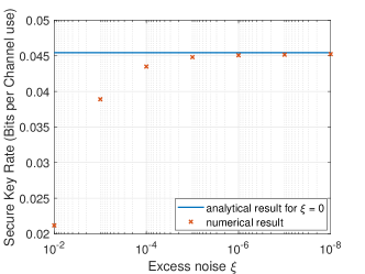
(a) Key rate vs excess noise $\xi$ compared to loss-only channel for $2$ Bobs where both are trusted.

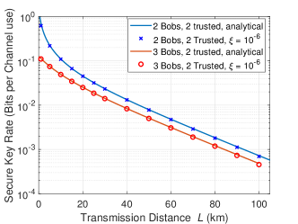
(b) Key rate vs transmission distance for $\xi=10^{-6}$ compared to loss-only channel.

Figure 8: Comparison of the numerical method to analytical benchmark for a QPSK protocol.

Appendix B Verification of the Numerical Method

This section briefly compares our numerical implementation to the analytical loss-only results. In Figure 8a, we fix the transmission distance to $L=20$km and the coherent state amplitude to $\alpha=0.87$ (which was the optimal $\alpha$ found for the loss-only case) and plot the obtained secure key rate for decreasing values of excess noise. The key rates converge to the analytical result for $\xi=0$, with negligible difference for $\xi=10^{-6}$ and lower. We note that we cannot choose $\xi$ exactly zero for numerical reasons. Next, in Figure 8b, we fix the excess noise to $\xi=10^{-6}$ and plot the secure key rate for 2 Bobs where both are trusted and 3 Bobs where 2 of them are trusted for various distances in the interval $[0\textrm{km},100\textrm{km}]$ and optimize over $\alpha$ in steps of $\Delta\alpha=0.01$ around the analytical optimum. Again, we compare our numerical results with the analytical result for the loss-only case and observe excellent accordance. Both Figures show the excellent alignment of our numerical results for the lossy & noisy case with the analytical loss-only key rates.

References

- Bennett and Brassard [1984] C. H. Bennett and G. Brassard, Quantum cryptography: Public key distribution and coin tossing, in Proceedings of IEEE International Conference on Computers, Systems, and Signal Processing (IEEE, India, 1984) p. 175.
- Ekert [1991] A. K. Ekert, Quantum cryptography based on Bell’s theorem, Phys. Rev. Lett. 67, 661 (1991).
- Ralph [1999] T. C. Ralph, Continuous variable quantum cryptography, Phys. Rev. A 61, 010303 (1999).
- Cerf et al. [2001] N. J. Cerf, M. Lévy, and G. V. Assche, Quantum distribution of Gaussian keys using squeezed states, Phys. Rev. A 63, 052311 (2001).
- Grosshans et al. [2003] F. Grosshans, J. Wenger, R. Tualle-Brouri, P. Grangier, G. Assche, and N. Cerf, Quantum key distribution using Gaussian-modulated coherent states, Nature 421, 238–241 (2003).
- Grosshans and Grangier [2002] F. Grosshans and P. Grangier, Continuous Variable Quantum Cryptography Using Coherent States, Phys. Rev. Lett. 88, 057902 (2002).
- Silberhorn et al. [2002] C. Silberhorn, T. C. Ralph, N. Lütkenhaus, and G. Leuchs, Continuous Variable Quantum Cryptography: Beating the 3 dB Loss Limit, Phys. Rev. Lett. 89, 167901 (2002).
- Navascués et al. [2006] M. Navascués, F. Grosshans, and A. Acín, Optimality of Gaussian Attacks in Continuous-Variable Quantum Cryptography, Phys. Rev. Lett. 97, 190502 (2006).
- García-Patrón and Cerf [2006] R. García-Patrón and N. J. Cerf, Unconditional Optimality of Gaussian Attacks against Continuous-Variable Quantum Key Distribution, Phys. Rev. Lett. 97, 190503 (2006).
- Diamanti and Leverrier [2015] E. Diamanti and A. Leverrier, Distributing Secret Keys with Quantum Continuous Variables: Principle, Security and Implementations, Entropy 17, 6072–6092 (2015).
- Leverrier et al. [2013] A. Leverrier, R. García-Patrón, R. Renner, and N. J. Cerf, Security of Continuous-Variable Quantum Key Distribution Against General Attacks, Phys. Rev. Lett. 110, 030502 (2013).
- Leverrier [2017] A. Leverrier, Security of continuous-variable quantum key distribution via a gaussian de finetti reduction, Phys. Rev. Lett. 118, 200501 (2017).
- Heid and Lütkenhaus [2006] M. Heid and N. Lütkenhaus, Efficiency of coherent-state quantum cryptography in the presence of loss: Influence of realistic error correction, Phys. Rev. A 73, 052316 (2006).
- Zhao et al. [2009] Y.-B. Zhao, M. Heid, J. Rigas, and N. Lütkenhaus, Asymptotic security of binary modulated continuous-variable quantum key distribution under collective attacks, Phys. Rev. A 79, 012307 (2009).
- Sych and Leuchs [2010] D. Sych and G. Leuchs, Coherent state quantum key distribution with multi letter phase-shift keying, New J. of Phys. 12, 053019 (2010).
- Ghorai et al. [2019] S. Ghorai, P. Grangier, E. Diamanti, and A. Leverrier, Asymptotic Security of Continuous-Variable Quantum Key Distribution with a Discrete Modulation, Phys. Rev. X 9, 021059 (2019).
- Lin et al. [2019] J. Lin, T. Upadhyaya, and N. Lütkenhaus, Asymptotic Security Analysis of Discrete-Modulated Continuous-Variable Quantum Key Distribution, Phys. Rev. X 9, 041064 (2019).
- Lin and Lütkenhaus [2020] J. Lin and N. Lütkenhaus, Trusted Detector Noise Analysis for Discrete Modulation Schemes of Continuous-Variable Quantum Key Distribution, Phys. Rev. Appl. 14, 064030 (2020).
- Upadhyaya et al. [2021] T. Upadhyaya, T. van Himbeeck, J. Lin, and N. Lütkenhaus, Dimension Reduction in Quantum Key Distribution for Continuous- and Discrete-Variable Protocols, PRX Quantum 2, 020325 (2021).
- Denys et al. [2021] A. Denys, P. Brown, and A. Leverrier, Explicit Asymptotic Secret Key Rate of Continuous-Variable Quantum Key Distribution with an Arbitrary Modulation, Quantum 5, 540 (2021).
- Matsuura et al. [2021] T. Matsuura, K. Maeda, T. Sasaki, and M. Koashi, Finite-size security of continuous-variable quantum key distribution with digital signal processing, Nat. Commun. 12, 252 (2021).
- Kanitschar and Pacher [2022] F. Kanitschar and C. Pacher, Optimizing continuous-variable quantum key distribution with phase-shift keying modulation and postselection, Phys. Rev. Applied 18, 034073 (2022).
- Lupo and Ouyang [2022] C. Lupo and Y. Ouyang, Quantum Key Distribution with Nonideal Heterodyne Detection: Composable Security of Discrete-Modulation Continuous-Variable Protocols, PRX Quantum 3, 010341 (2022).
- Kanitschar et al. [2023] F. Kanitschar, I. George, J. Lin, T. Upadhyaya, and N. Lütkenhaus, Finite-size security for discrete-modulated continuous-variable quantum key distribution protocols, PRX Quantum 4, 040306 (2023).
- Bäuml et al. [2023] S. Bäuml, C. P. García, V. Wright, O. Fawzi, and A. Acín, Security of discrete-modulated continuous-variable quantum key distribution (2023), arXiv:2303.09255 [quant-ph] .
- Cabello [2000] A. Cabello, Multiparty key distribution and secret sharing based on entanglement swapping (2000), arXiv:quant-ph/0009025 [quant-ph] .
- Chen and Lo [2008] K. Chen and H.-K. Lo, Multi-partite quantum cryptographic protocols with noisy ghz states (2008), arXiv:quant-ph/0404133 [quant-ph] .
- Epping et al. [2017] M. Epping, H. Kampermann, C. macchiavello, and D. Bruß, Multi-partite entanglement can speed up quantum key distribution in networks, New Journal of Physics 19, 093012 (2017).
- Grasselli et al. [2018] F. Grasselli, H. Kampermann, and D. Bruß, Finite-key effects in multipartite quantum key distribution protocols, New Journal of Physics 20, 113014 (2018).
- Murta et al. [2020] G. Murta, F. Grasselli, H. Kampermann, and D. Bruß, Quantum conference key agreement: A review, Advanced Quantum Technologies 3, 10.1002/qute.202000025 (2020).
- Bian et al. [2023] Y. Bian, Y.-C. Zhang, C. Zhou, S. Yu, Z. Li, and H. Guo, High-rate point-to-multipoint quantum key distribution using coherent states (2023), arXiv:2302.02391 [quant-ph] .
- Hajomer et al. [2024] A. A. E. Hajomer, I. Derkach, R. Filip, U. L. Andersen, V. C. Usenko, and T. Gehring, Continuous-variable quantum passive optical network (2024), arXiv:2402.16044 [quant-ph] .
- Coles et al. [2016] P. J. Coles, E. M. Metodiev, and N. Lütkenhaus, Numerical approach for unstructured quantum key distribution, Nat. Commun. 7, 11712 (2016).
- Winick et al. [2018] A. Winick, N. Lütkenhaus, and P. J. Coles, Reliable numerical key rates for quantum key distribution, Quantum 2, 77 (2018).
- Kanitschar [2021] F. P. Kanitschar, Postselection Strategies for CV-QKD protocols with Phase-Shift Keying Modulation, Master’s thesis, TU Wien (2021).
- Devetak and Winter [2005] I. Devetak and A. Winter, Distillation of secret key and entanglement from quantum states, Proc. R. Soc. A 461, 207 (2005).
- Curty et al. [2004] M. Curty, M. Lewenstein, and N. Lütkenhaus, Entanglement as a Precondition for Secure Quantum Key Distribution, Phys. Rev. Lett. 92, 217903 (2004).
- Ferenczi and Lütkenhaus [2012] A. Ferenczi and N. Lütkenhaus, Symmetries in quantum key distribution and the connection between optimal attacks and optimal cloning, Phys. Rev. A 85, 052310 (2012).
- Upadhyaya [2021] T. Upadhyaya, Tools for the Security Analysis of Quantum Key Distribution in Infinite Dimensions, Master’s thesis (2021).
- Frank and Wolfe [1956] M. Frank and P. Wolfe, An algorithm for quadratic programming, Nav. Res. Logist. Q. 3, 95 (1956).
- Grant and Boyd [2014] M. Grant and S. Boyd, CVX: Matlab Software for Disciplined Convex Programming, version 2.1, http://cvxr.com/cvx (2014).
- Grant and Boyd [2008] M. Grant and S. Boyd, Graph implementations for nonsmooth convex programs, in Recent Advances in Learning and Control, Lecture Notes in Control and Information Sciences, edited by V. Blondel, S. Boyd, and H. Kimura (Springer-Verlag Limited, London, 2008) pp. 95–110, http://stanford.edu/~boyd/graph_dcp.html.
- ApS [2019] M. ApS, The MOSEK optimization toolbox for MATLAB manual. Version 9.0. (2019).
- Coles [2012] P. J. Coles, Unification of different views of decoherence and discord, Physical Review A 85, 10.1103/physreva.85.042103 (2012).
- Leverrier [2023] A. Leverrier, Information reconciliation for discretely-modulated continuous-variable quantum key distribution (2023), arXiv:2310.17548 [quant-ph] .
- Bergmayr et al. [2023] A. Bergmayr, F. Kanitschar, M. Pivoluska, and M. Huber, How to harness high-dimensional temporal entanglement, using limited interferometry setups (2023), arXiv:2308.04422 [quant-ph] .
- Kanitschar [2022] F. P. Kanitschar, Finite-size security proof for discrete-modulated CV-QKD protocols, Master’s thesis, TU Wien (2022).