IFT-UAM/CSIC-24-92

On small Dirac Neutrino Masses
in String Theory
Gonzalo F. Casas,^♢ Luis E. Ibáñez^♣♢ and Fernando Marchesano^♢
♣ Departamento de Física Teórica
Universidad Autónoma de Madrid, Cantoblanco, 28049 Madrid, Spain
^♢ Instituto de Física Teórica UAM-CSIC, c/ Nicolas Cabrera 13-15, 28049 Madrid, Spain
Abstract

We study how tiny Dirac neutrino masses consistent with experimental constraints can arise in string theory SM-like vacua. We use as a laboratory 4d ${\cal N}=1$ type IIA Calabi–Yau orientifold compactifications, and in particular recent results on Yukawa couplings at infinite field-space distance. In this regime we find Dirac neutrino masses of the form $m_{\nu}\simeq g_{\nu}\langle H\rangle$, with $g_{\nu}$ the gauge coupling of the massive $U(1)$ under which the right-handed neutrinos $\nu_{R}$ are charged, and which should be in the range $g_{\nu}\simeq 10^{-14}-10^{-12}$ to reproduce neutrino data. The neutrino mass suppression occurs because the right-handed neutrino kinetic term behaves as $K_{\nu\nu}\simeq 1/g_{\nu}^{2}$. At the same time a tower of $\nu_{R}$-like states appears with characteristic scale $m_{0}\simeq g_{\nu}^{2}M_{\rm P}\simeq 0.1-500$ eV, in agreement with Swampland expectations. Two large hidden dimensions only felt by the $\nu_{R}$ sector arise at the same scale, while the string scale is around $M_{s}\simeq g_{\nu}M_{\rm P}\simeq 10-700$ TeV. Some phenomenological implications and model building challenges are described. As a byproduct, independently of the neutrino issue, we argue that a single large dimension in the context of SM-like type IIA Calabi–Yau orientifolds leads to too small Yukawa couplings for quarks and charged leptons.

1 Introduction

Neutrinos remain possibly the most mysterious particles of the Standard Model (SM) (for a recent review see e.g. [1, 2] and references therein). We still do not know whether they are Dirac or Majorana particles and what is the origin of their tiny mass. In fact, we still cannot rule out one of the three neutrino types being massless, and we ignore whether there is a normal hierarchy (NH) or an inverted hierarchy (IH) in their mass pattern. Depending on the origin of their mass, two main possibilities arise:

• Dirac masses. In this case it is assumed that there are both left-handed $\nu_{L}$ (in a $SU(2)_{L}$ doublet) and right-handed $\nu_{R}$ (SM singlet) neutrinos, both initially massless. They couple to the Higgs boson through Yukawa couplings $Y_{\nu}$ and once the Higgs gets a vev they get Dirac masses given by

  $$m_{\nu}^{\rm Dirac}\,\simeq\,Y_{\nu}\langle H_{0}\rangle\,.$$ (1.1)

  Here $Y_{\nu}$ are Yukawa couplings which should be tiny, in the range $10^{-12}-10^{-13}$, in order to match the experimental oscillation data, and $\langle H_{0}\rangle$ is the Higgs vev.

• Majorana masses. One may consider such tiny Yukawa couplings to be fine-tuned, which would be nice to avoid. A natural way in which tiny Yukawa couplings are avoided is the celebrated ‘see-saw mechanism’ [3, 4, 5]. Since the $\nu_{R}$’s are SM singlets they may be arbitrarily heavy, perhaps with masses $M_{R}$ of order some UV scale, so that $M_{R}\gg M_{EW}$. This structure leads to the well-known expression for Majorana masses of order

  $$m_{\nu}^{\rm Majorana}\,\simeq\,\frac{\left(Y_{\nu}\langle H_{0}\rangle\right)^{2}}{M_{R}}\,,$$ (1.2)

  which for ordinary Yukawa couplings of order $10^{-4}-10^{-1}$ will give masses consistent with experiment for $M_{R}\sim 10^{14}$ GeV. These eigenstates are predominantly coming from the $\nu_{L}$’s and have Majorana masses.

It is interesting to explore how, if at all, these two mechanisms arise in string theory. A fruitful strategy to explore these question has been to consider string compactifications based in type IIA CY orientifolds with intersecting D6-branes (see e.g. [6, 7, 8, 9, 10, 11, 12] and references therein), and this is the class of theories that we will use in this paper as a laboratory. Due to different dualities transforming this class of vacua to other corners in the 4d ${\cal N}=1$ landscape, we believe that the results we obtain are rather generic in the space of realistic string vacua.

Large $\nu_{R}$ Majorana masses in string theory

The simplest setup assumes type IIA CY orientifold vacua close to the SM physics, with $3+2+n$ stacks of intersecting D6-branes giving rise to a $U(3)\times U(2)\times U(1)^{n}$, $n\geq 2$ gauge group. The subgroup $U(1)^{n+2}$ contains the hypercharge and the rest of the $U(1)$’s become generically massive from $B\wedge F$ couplings, inducing Stükelberg masses for them. Here $B$ are 2-forms arising from the gravitational sector of the theory. The extra, massive $U(1)$’s include lepton and baryon numbers which are thus gauged. The spectrum always includes perturbatively massless right-handed neutrinos $\nu_{R}$. However, it was shown [13, 14, 15] that once the lepton number gets massive due to a $B\wedge F$ coupling, $\nu_{R}$ Majorana masses may be induced by ‘charged stringy instantons’. These correspond to Euclidean $D2$-branes wrapping 3-cycles in the internal manifold and intersecting the branes that localise the $\nu_{R}$’s [13, 14, 15]. The induced masses are of order

$$m_{\nu_{R}}\,\simeq\,M_{s}\,e^{-S_{E}}\,\simeq\,M_{s}\,e^{-u_{E}}\ ,$$ (1.3)

where $M_{s}$ is the string scale and $S_{E}$ is the instanton action, whose size is determined by a complex structure scalar $u_{E}$ that measures the volume of the 3-cycle wrapped by the instanton $E2$ in string units. If this volume is not large and we have a high string scale around $M_{s}\simeq 10^{16}$ GeV, one may obtain large Majorana masses for the right-handed neutrinos in the range consistent with experiment. This is an elegant mechanism. Still it turns out that the conditions for such instantons to produce a mass term in specific string vacua are not so easy to attain. In particular, it turns out that typically there are additional instanton ‘neutral zero modes’ in the theory which often lead to vanishing amplitudes for a mass term. In particular, in [16] a search was made in a large class of type II 4d ${\cal N}=1$ SM-like orientifolds obtained from rational CFT’s (Gepner-like models). It was found no example in which the required structure of zero modes to get $\nu_{R}$ Majorana masses exists. This should not be considered as a sort of ‘no-go theorem’ since the class of theories studied was large but certainly not exhaustive. Furthermore additional effects like closed string fluxes may get rid of some unwanted singlet zero modes, allowing for masses to be generated. Nevertheless, this motivates to study whether the Dirac mass alternative is viable in string theory.

Tiny Dirac neutrino masses in string theory

This is the alternative that we study in the present paper. Note that within a given string vacuum three conditions are then required: 1) There must exist some limit in moduli space in which tiny Dirac masses for all neutrinos are obtained. This limit must be such that 2) the Yukawa couplings as well as the SM gauge couplings remain unsuppressed for the rest of the fermions, quarks and charged leptons, while 3) right-handed Majorana neutrino masses are very small or vanishing. It turns out that this third condition is essentially automatic, once the other two are achieved. On the contrary, we find that the two first conditions are very strong and almost uniquely fix how the structure of mass scales must be in a string vacuum in order to get viable Dirac neutrino masses. The subject of the first condition has been recently addressed in the paper [17] in which it has been studied the behaviour of matter Yukawa couplings at large moduli, leading to vanishing small Yukawa couplings. There it was found that the Yukawa couplings among three chiral matter fields living at D6-brane intersections $i,j,k$ have the general structure

$$Y_{ijk}\,=\,\frac{W_{ijk}}{{\rm Vol}_{X}^{1/2}}e^{\phi_{4}/2}\Theta_{ijk}^{1/4}\,.$$ (1.4)

On the one hand, ${\rm Vol}_{X}$ is the volume of the compact manifold in units of $M_{s}$ and $W_{ijk}$ is the holomorphic superpotential, both depending only on the complexified Kähler moduli $T^{a}$. On the other hand $\phi_{4}$ is the 4d dilaton and the functions $\Theta_{ijk}$ encode the information about the intersection angles of the three D6-branes involved in the Yukawa coupling, both quantities depending only on the complex structure fields $u^{K}$. As pointed out in [17], the interesting limit for us will be the one in which we keep the Kähler moduli fixed and ${\rm Vol}_{X}$ is not too large, since the ${\rm Vol}_{X}\rightarrow\infty$ corresponds to an M-theory limit in which we are not interested. Alternatively, perturbative limits with vanishing Yukawas imply some complex structure fields becoming large. In a limit parametrised by a single complex structure direction $u\rightarrow\infty$, Yukawa couplings behave like $Y\simeq 1/u^{r}$ with $r$ some rational number typically in the range $1/4\leq r\leq 1$ [17]. At the same time towers of light states with the same quantum numbers as the massless quarks and leptons, termed ‘gonions’ in [18], become light.

In the case of neutrinos, the crucial issue is to obtain tiny neutrino Yukawa couplings while the rest of Yukawa couplings as well as the SM gauge couplings, remain unsuppressed. We find that in the context of type II CY SM-like orientifolds, tiny Yukawa couplings require the presence of $\nu_{R}$ gonion towers becoming light as $m_{{\rm gon},\nu_{R}}\sim M_{\rm P}/u$ while two dimensions become large at the same rate. The appearance of precisely two large dimensions is a consequence of requiring that i) only neutrinos get very suppressed Yukawa couplings and ii) the string scale $M_{s}$ is compatible with experiment. This is essentially because all the relevant scales of this scenario have simple behaviour in terms of $u$. In particular, the neutrino Yukawa couplings behave like $Y_{\nu}\sim u^{-1/2}$, which is also the rate of variation $g_{\nu}\sim u^{-1/2}$ of the gauge coupling associated with the massive $U(1)_{\nu}$ gauge interaction felt by right-handed neutrinos. The fundamental scales of the theory are then determined in terms of the neutrino couplings as

$$M_{s} \simeq Y_{\nu}M_{\rm P}\,\simeq\,g_{\nu}M_{\rm P}\,,$$ (1.5)

$$m_{{\rm gon},\nu_{R}} \simeq m_{{\rm KK}}\,\simeq\,Y_{\nu}^{2}\,M_{\rm P}\,\simeq\,g_{\nu}^{2}\,M_{\rm P}\,,$$ (1.6)

where $Y_{\nu}$ here is the largest of the neutrino Yukawa couplings. Setting $Y_{\nu}\simeq 7\times 10^{-13}$, consistent with neutrino oscillations data, gives

$$M_{s}\simeq 700\ {\rm TeV}\,,\qquad m_{{\rm gon},\nu_{R}}\,\simeq\,m_{{\rm KK}}\,\simeq\,500\,{\rm eV}\,.$$ (1.7)

As a result the string scale is lowered to a scale well above, but not far away, from the EW scale. In addition there are two large dimensions around the 500 eV, along with a tower of $\nu_{R}$-like states. There is also an extra $U(1)_{\nu}$ with very weak coupling $g_{\nu}\sim 10^{-14}-10^{-12}$ with a mass $M_{V_{\nu}}$ in the wide range $0.1\,{\rm eV}\leq M_{V_{\nu}}\leq M_{s}$. In fact, if the $\nu_{R}$ gonion towers are not universal, the scales may be lowered down to the values

$$M_{s}\simeq 10\ {\rm TeV}\,,\qquad m_{{\rm gon},\nu_{R}}\,\simeq\,m_{{\rm KK}}\,\simeq\,0.1\,{\rm eV}\ ,$$ (1.8)

not far above LHC bounds for the string scale: $M_{s}\lesssim 8$ TeV. We briefly discuss possible phenomenological implications of the above spectrum of new particles in section 4. The obtained structure may be considered as a concrete string theory realisation of the Large Extra Dimension (LED) scenario of [19] and neutrino masses in this setting [20]. However, as seen above, the embedding into a string theory lead us to a very concrete scenario in which two dimensions must be large and the relevant mass scales display a very specific structure.

The results obtained for the mass scales and towers of states in these types of compactifications are, as expected, consistent with general Swampland arguments (see [21, 22, 23, 24] for reviews). In particular light towers of states are obtained along large complex structure limits, in agreement with the Swampland Distance Conjecture (SDC), and such towers obey the Weak Gravity Conjecture (WGC) for the $U(1)_{\nu}$ gauge boson coupling to $\nu_{R}$’s. In fact there are arguments, based on the AdS instability conjecture [25, 26] which states that neutrinos must be Dirac and the lightest neutrino must have a mass bounded by the cosmological constant scale, $m_{\nu}^{\rm min}\lesssim\Lambda_{{\rm cc}}^{1/2}$ [27, 28, 29]. This nicely fits with the Dirac option which we analyse in this paper. We describe some consequences of these Swampland arguments in section 5. In combination with our previous results, they give a rationale for why two large dimensions should open: they are required to obtain a sufficiently light Dirac neutrino to obey the Swampland bound $m_{\nu}^{\rm min}\lesssim\Lambda_{{\rm cc}}^{1/4}$. This also explains the apparent coincidence between the neutrino mass scale and that of the cosmological constant.

The structure of the rest of the paper is as follows. In section 2, we give a short introduction to type IIA ${\cal N}=1$ CY orientifolds with intersecting D6-branes. We describe the spectrum in this class of theories and the structure of asymptotically vanishing Yukawa couplings. We also provide an explicit example that illustrates the general limiting structure of mass scales and Yukawas. In section 3 we give a D6-brane configuration whose intersections contain the massless chiral fields of the SUSY SM and Higgs fields. We discuss how tiny Yukawa couplings for neutrinos may be obtained in a setting with two large dimensions, and describe the general structure of scales and the mass of the extra $U(1)$’s. In section 4 we impose that the obtained value for the neutrino Yukawa couplings agrees with neutrino data, which essentially fixes all scales. We also give a brief description of possible phenomenological implications. In section 5 we briefly describe how the results obtained fit within general Swampland arguments and in particular the implications of the upper bound on the lightest neutrino mass coming from the 3d SM compactification and the AdS instability conjecture. Some final comments are left for section 6.

Some technical details have been relegated to three appendices. In appendix A we explain the difficulties of having a SM-like orientifold with a single large dimension and only the neutrino Yukawa couplings small, and then rule out settings with more than two large dimensions because they imply a very small string scale. In appendix B we present an $SU(5)$ intersection brane setting in which the same general structure for obtaining tiny Yukawa couplings is realised. Appendix C contains an analysis of the $U(1)$ anomalies and the conditions for $U(1)$’s other than hypercharge becoming massive in the explicit SM-like configuration described in the main text.

2 4d ${\cal N}=1$ type IIA orientifolds as a laboratory

In this section we first briefly review the construction of type IIA ${\cal N}=1$ CY orientifolds with intersecting D6-branes. We then describe the structure of matter field Yukawa couplings and their behavior for large moduli, leading to the search for small Yukawa couplings. The main characteristics of these constructions at infinite distance are illustrated in a $\mathbbm{Z}_{2}\times\mathbbm{Z}_{2}$ toy model with a Pati-Salam structure. We also describe the difficulties in getting a compactification with only one large dimension if we want to keep unsuppressed the SM gauge and Yukawa couplings other than neutrino’s.

2.1 Type IIA orientifolds and intersecting D6-branes

Let us sketch the basic properties of the string theory construction that we will use to analyse Yukawa couplings, namely type IIA Calabi–Yau (CY) orientifolds with intersecting D6-branes. A detailed description of this class of vacua and their phenomenology can be found in the reviews [6, 7, 8, 9, 10, 11, 12] as well as in [17, section 2.1], whose conventions and notation we will follow.

Calabi–Yau orientifold vacua are built on a background of the form $X_{4}\times X_{6}$, where $X_{4}$ are four macroscopic dimensions and $X_{6}$ are six extra dimensions curled up in a compact manifold with a CY metric. One then imposes a parity-reversal $\mathbbm{Z}_{2}$ quotient to the worldsheet of strings propagating in this background. In terms of 10d geometry, this translates into a quotient by an involution ${\cal R}$ acting on $X_{6}$ and leaving $X_{4}$ invariant. In type IIA CY orientifolds, this action is given by ${\cal R}(J,\Omega)=(-J,\bar{\Omega})$, where $J$ is the Kähler form and $\Omega$ the holomorphic three-form that determine the CY metric on $X_{6}$. The fixed point set of ${\cal R}$ is of the form $X_{4}\times\Pi_{\rm O6}$, with $\Pi_{\rm O6}$ either one or a sum of smooth three-cycles, where the O6-plane content of the compactification is located. To achieve a consistent background one needs to cancel the internal charge induced by the O6-planes, for instance by adding stacks of $N_{\alpha}$ D6-branes on $X_{4}\times\Pi_{\alpha}$, where $\Pi_{\alpha}$ are a set of three-cycles such that $\sum_{\alpha}N_{\alpha}\left([\Pi_{\alpha}]+[\Pi_{\alpha*}]\right)=4[\Pi_{\rm O6}]$. Here the brackets denote their homology classes in $H_{3}(X_{6},\mathbbm{Z})$ and $\Pi_{\alpha*}={\cal R}(\Pi_{\alpha})$ stands for the orientifold image of each D6-brane. To insure instability, one typically requires a BPS condition for the $\Pi_{\alpha}$, namely that they are special Lagrangian three-cycles with no worldvolume flux.

The 4d EFT obtained from this compactification has an open and a closed string sector, each of them hosting a set of light fields. Closed strings give rise to the 4d ${\cal N}=1$ gravity multiplet, as well as a set of chiral multiplets whose bosonic components describe the internal geometry of $X_{6}$. These are the Kähler $T^{a}=b^{a}+it^{a}$ and complex structure $U^{K}=\zeta^{K}+iu^{K}$ moduli. The real part of these fields are periodic axionic variables, while the imaginary part are saxion fields that describe the geometry of $X_{6}$ in terms of $J$ and $\mbox{Re}\,\Omega$, respectively. They also determine the kinetic terms of the closed string sector, via the Kähler potential $K\equiv K_{K}+K_{Q}$, where [31]

$$K_{K}\equiv-{\rm log}\left({\rm Vol}_{X_{6}}\right)=-{\rm log}\left(\frac{i}{48}{\cal K}_{abc}(T^{a}-\bar{T}^{a})(T^{b}-\bar{T}^{b})(T^{c}-\bar{T}^{c})\right)\,,$$ (2.1)

with ${\cal K}_{abc}\equiv\ell_{s}^{-6}\int_{X_{6}}\omega_{a}\wedge\omega_{b}\wedge\omega_{c}$ the triple intersection numbers of $X_{6}$ and

$$K_{Q}\equiv-2\log{\cal H}=-2\log\left(\frac{i}{8\ell_{s}^{6}}\int_{X_{6}}e^{-2\phi}\Omega\wedge\bar{\Omega}\right)=4\phi_{4}\,,$$ (2.2)

with $\phi_{4}=\phi-\frac{1}{2}\log{\rm Vol}_{X_{6}}$ the 4d dilaton and $\phi$ the 10d dilaton.

Non-Abelian gauge group	$\prod_{\alpha}SU(N_{\alpha})$
Massless $U(1)$s	$\sum_{\alpha}c_{\alpha}U(1)_{\alpha}$ such that $\sum_{\alpha}c_{\alpha}([\Pi_{\alpha}]-[\Pi_{\alpha*}])=0$
Chiral multiplets	$\sum_{\alpha<\beta}\,I_{\alpha\beta}({\bf N}_{\alpha},{\bf\bar{N}}_{\beta})\,+\,I_{\alpha\beta*}({\bf N}_{\alpha},{\bf\bar{N}}_{\beta})$

Table 1: 4d EFT chiral spectrum, in terms of the intersection number $I_{\alpha\beta}=[\Pi_{\alpha}]\cdot[\Pi_{\beta}]$. For simplicity we assume that $I_{\alpha\alpha*}=I_{\alpha{\rm O6}}=0$, as in the models of section 3. If $\Pi_{\alpha}=\Pi_{\alpha*}$, the D6-brane hosts either an $SO(2N_{\alpha})$ or $USp(2N_{\alpha})$ gauge group.

The massless open string states oscillations give rise the gauge sector of the 4d EFT, which is localised at the D6-brane worldvolume and their intersections. More precisely, the net 4d chiral spectrum is specified by the topological intersection number $I_{\alpha\beta}=[\Pi_{\alpha}]\cdot[\Pi_{\beta}]$ between pairs of three-cycles wrapped by D6-branes, as summarised in table 1. Each transverse intersection between two three-cycles localises a 4d chiral fermion at a point in $X_{6}$, together with an infinite tower of massive particles with the same bifundamental charges [32, 33]. These massive states were dubbed gonions in [18], and they are particularly relevant in models with very small intersection angles .

The gonion tower spectrum can be different at each intersection, depending on the local geometry. In the generic case of a transverse intersection, it is specified by three intersection angles $\theta_{\alpha\beta}^{r}$ $r=1,2,3$, measured in units of $\pi$. Whenever one or more angles are small the tower displays a spectrum of the form [32, 33]

$$m_{\alpha\beta}^{2}=\sum_{q}k_{q}|\theta_{ab}^{q}|M_{s}^{2}\,,$$ (2.3)

up to an angle-dependent function that depends on whether we are talking about a charged scalar, fermion or W-boson. Here $q$ runs over those angles that satisfy $|\theta_{ab}^{q}|\ll 1$, $k_{q}\in\mathbbm{N}$ and $M_{s}=e^{\phi_{4}}M_{\rm P}$ is the string scale. We will be mainly interested in setups with a single small angle, in which case this tower is as dense as a two-dimensional lattice of KK modes. At the string scale, additional states appear, so that one recovers a Hagedorn-like spectrum, see figure 1 and [17, Appendix A].

Figure 1: Gonion tower spectrum with one small angle $\theta_{\alpha\beta}$. There is a tower of gonions with the same charge as the massless mode $\Phi_{\alpha\beta}$ and characteristic mass $m_{{\rm gon},\alpha\beta}$. The tower runs up to the string scale $M_{s}$, at which a Hagedorn spectrum is recovered.

The interplay between open and closed string sectors manifests in a set of gauge kinetic functions that depend linearly on the complex structure moduli $U^{K}$, and a generalised Green–Schwarz (GS) mechanism that cancels $U(1)$ anomalies and implements a Stückelberg mechanism on them [33, 39]. The explicit expressions are obtained from expanding the three-cycles homology classes wrapped by the D6-branes as $[\Pi_{\alpha}]=P_{\alpha\,J}[\Sigma^{J}_{+}]+Q_{\alpha}^{K}[\Sigma_{K}^{-}]$, where $[\Sigma^{J}_{+}]$ is a certain basis of even and $[\Sigma_{K}^{-}]$ of odd classes under the action of ${\cal R}$, satisfying $[\Sigma_{K}^{-}]\cdot[\Sigma^{J}_{+}]=2\delta^{J}_{K}$, and $P_{\alpha\,J}$, $Q_{\alpha}^{K}$ are integers or half-integers. Then the gauge coupling associated with each stack is

$$\frac{2\pi}{g_{\alpha}^{2}}=P_{\alpha\,K}u^{K}\,,$$ (2.4)

and the Stückelberg mass for the $U(1)$’s involved in the GS mechanism reads [40]

$$M_{\alpha\beta}^{2}=4G_{KL}Q^{K}_{\alpha}Q^{L}_{\beta}g_{\alpha}g_{\beta}\,M_{\rm P}^{2}\,.$$ (2.5)

Finally, supersymmetry implies that there is a D-term potential for the chiral fields charged under the massive $U(1)$’s, which reads

$$V_{D}=\frac{1}{2}\sum_{\alpha}g_{\alpha}^{2}\left(\xi_{\alpha}+\sum_{i}q^{i}_{\alpha}K_{i\bar{i}}\Phi_{i}\bar{\Phi}_{\bar{i}}\right)^{2}\,,\qquad\text{with}\quad\pi\xi_{\alpha}=Q^{K}_{\alpha}\ell_{K}M_{\rm P}^{2}\,.$$ (2.6)

Here $\Phi_{i}$ represents the scalar component of the 4d chiral field at two D6-brane intersections, with kinetic terms $K_{i\bar{i}}$ and charge $q^{i}_{\alpha}$ under $U(1)_{\alpha}$, and $\xi_{\alpha}$ is the Fayet-Iliopoulos term [41], which is a linear combination of the dual saxions defined as $\ell_{K}=-\partial_{u^{K}}K$. Interestingly, it was found in [17] that the vev of such dual saxions may provide a rough estimate of the gonion tower scale, via

$$m_{{\rm gon},\alpha\beta}\sim g_{\rm min}\ell_{\rm min}^{1/2}M_{\rm P}\,,$$ (2.7)

where $g_{\rm min}={\rm min}(g_{\alpha},g_{\beta})$ and $\ell_{\rm min}$ is the smallest dual saxion involved in the FI-term of such $U(1)$. See [17] for a more precise discussion and applications to specific setups.

2.2 Yukawas at infinite distance

Standard trilinear Yukawa couplings in type IIA CY orientifolds correspond to string amplitudes involving three D6-branes intersecting at angles at a single point in the CY, or connected through a worldsheet along a triangle joining three intersections of the involved D6-branes [18], see fig.(2). Those Yukawa couplings have been computed explicitly for toroidal or orbifold compactifications, see [42, 43, 44, 45, 46, 47]. The generic CY case is obviously more involved, but due to the locality of the interactions, some general results for the Yukawa couplings can nevertheless be obtained. Here we summarise some of the results in [17] concerning Yukawa couplings at infinite field distance, in particular concerning the large complex structure limit in type IIA CY orientifolds. In this reference it was argued that canonically normalised Yukawa couplings among matter fields at D6-brane intersections, labelled by the family indices $i,j,k$ are given by an expression of the form

$$Y_{ijk}\ =\ \frac{W_{ijk}}{{\rm Vol}_{X}^{1/2}}e^{\phi_{4}/2}\Theta_{ijk}^{1/4}\ .$$ (2.8)

Here $W_{ijk}$ is the holomorphic superpotential coupling, which is a function of the Kähler moduli, and $\phi_{4}$ is the 4d dilaton. The functions $\Theta_{ijk}$ contain all the information about the local angles of intersection of the different $D6$-branes, see e.g. ref.[17] for details and toroidal examples. Finally ${\rm Vol}_{X}$ is the volume of the compact CY three-fold $X_{6}$, which is a function of the Kähler moduli.

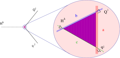
Figure 2: Yukawa couplings arise at the intersection of three D6-branes.

The challenge that we address in this work is to identify moduli space directions in which one can suppress the Yukawa couplings of neutrinos while maintaining unsuppressed (or not exceedingly suppressed) the rest of the SM Yukawa couplings. In this sense, notice that taking the limit ${\rm Vol}_{X}\rightarrow\infty$ is not a good strategy, since it affects all the Yukawas in a universal way. Furthermore, if we take this limit at constant or slowly varying $e^{\phi_{4}}$, then a KK-like tower of D0-branes becomes light, signalling a decompactification regime in which one extra dimension opens up, and the microscopic physics of the system is better described by M-theory on a $G_{2}$-manifold. A different strategy to get almost vanishing Yukawa couplings is to construct models in which the holomorphic Yukawas $W_{ijk}$ have some zero entries, which then get corrected by exponentially suppressed contributions from Euclidean E2-brane charged instantons, see refs.[13, 14, 15, 16, 48, 49, 50, 51]. However, in practice it is quite challenging to find explicit D6-brane models in which all neutrino Yukawas become very small while avoiding that some other quarks or charged lepton Yukawas also become small, see some attempts in [48, 49, 51] and references therein.

In the following we will apply a different line of action, based on the approach and results of our recent work [17], that explored the structure of Yukawas at fixed CY volume and and large vevs for the complex structure fields. Geometrically, this corresponds to considering cases in which some of the intersection angles involved in a certain Yukawa couplings become very small [17]. In those limits the structure of the said Yukawas reduces to the form

$$Y_{ijk}\,\simeq\,Be^{\phi_{4}/2}\Theta_{ijk}^{1/4}\,,$$ (2.9)

with $B$ taken to be an order one constant. In the case that all three vertices have three gonion towers one can write [17]

$$Y_{ijk}\,\sim\,e^{-\phi_{4}}\left(\frac{m_{\rm gon}^{i}}{M_{\rm P}}\cdot\frac{m_{\rm gon}^{j}}{M_{\rm P}}\cdot\frac{m_{\rm gon}^{k}}{M_{\rm P}}\right)^{1/2},$$ (2.10)

where the gonion scales correspond to the leading tower (if there is more than one) at each intersection. Along limits in which we send one or several saxions $u^{K}$ to infinity, we have that $e^{\phi_{4}}=M_{s}/M_{\rm P}\to 0$. Then, because we always have the hierarchy $m_{\rm gon}<M_{s}<M_{\rm P}$, (2.10) tends to zero as well. These are the infinite distance limits that were explored in [17] where it was argued that whenever $Y\to 0$ at least one of the gauge couplings involved in the Yukawa also tends to zero.

There is a particularly interesting case in which only one intersection (say, the $i^{\rm th}$) presents small angles. In that case the expression is simplified to

$$Y_{ijk}\,\sim\,e^{-\phi_{4}}\left(\frac{m_{\rm gon}^{i}}{M_{\rm P}}\right)^{1/2}\frac{M_{s}}{M_{\rm P}}\simeq\ \left(\frac{m_{\rm gon}^{i}}{M_{\rm P}}\right)^{1/2}\ ,$$ (2.11)

where we have used $M_{s}=e^{\phi_{4}}M_{\rm P}$. Thus in this case the Yukawa coupling is determined by the gonion scale of the intersection with the smallest angle. This will be the case of interest to obtain realistic Dirac neutrino masses, as it will apply to the neutrino sector Yukawas. For the rest of the Yukawas, the idea is that they involve at least one ${\cal N}=2$ sector, see footnote 3. Then, from (2.9) one obtains $Y_{ijk}\sim h_{i\bar{i}}^{-1/2}\left(\frac{m_{\rm gon}^{i}}{M_{s}}\cdot\frac{m_{\rm gon}^{j}}{M_{s}}\right)^{1/2}$ instead of (2.10), where $h_{i\bar{i}}$ is a function of the saxions $\{u^{K}\}$ bounded by $g_{\alpha}^{-1}g_{\beta}^{-1}$, namely the two gauge couplings involved in the ${\cal N}=2$ sector [17]. Because in this case there is no 4d dilaton suppression when expressing $Y_{ijk}$ in terms of ${m_{\rm gon}}/{M_{s}}$, these other Yukawas need not be suppressed along the infinite distance limits under consideration, allowing for a realistic set of couplings.

2.2.1 A toroidal orientifold toy model

To get a more detailed flavour of the structure of this limit we briefly consider here the toroidal orientifold example described in [17, section 4], see that reference for details and notation. It is obtained starting from a compact toroidal space $X_{6}=({\bf T}^{2})_{1}\times({\bf T}^{2})_{2}\times({\bf T}^{2})_{3}/\Gamma$, where $\Gamma={\bf Z}_{2}\times{\bf Z}_{2}$ has the same action as considered in [52, 53]. Each torus is parametrised by a complex coordinate $z_{i}=y_{2i-1}+i\tau_{i}\,y_{2i}$, $i=1,2,3$, where the geometric complex structure is $\tau_{i}=R_{2i}/R_{2i-1}$. The untwisted complex structure moduli have real parts given by

$$s=\frac{e^{-\phi}}{4}R_{1}R_{3}R_{5}\,,\quad u^{(1)}=\frac{e^{-\phi}}{4}R_{1}R_{4}R_{6}\,,\quad u^{(2)}=\frac{e^{-\phi}}{4}R_{2}R_{3}R_{6}\,,\quad u^{(3)}=\frac{e^{-\phi}}{4}R_{2}R_{4}R_{5},$$ (2.12)

with the 4d dilaton given by $e^{-2\phi_{4}}=4\sqrt{su^{(1)}u^{(2)}u^{(3)}}$, and the string scale reads $M_{s}=e^{\phi_{4}}M_{\rm P}$. For $\tau_{i}\ll 1$ there are KK and winding towers determined by the scales respectively

$$m_{{\rm KK},i}\,=\,\frac{2M_{s}}{R_{2i-1}}\,=\,\frac{M_{\rm P}}{2A_{i}^{1/2}\sqrt{su^{(i)}}}\,,\qquad m_{{\rm w},i}\,=\,\frac{1}{2}R_{2i}M_{s}\,=\,\frac{A_{i}^{1/2}M_{\rm P}}{2\sqrt{su^{(i)}}}\,,$$ (2.13)

where $A_{i}=(R_{2i}R_{2i-1})/4$ is the area of $({\bf T}^{2})_{i}$. We consider now stacks of $D6$-branes $D6_{a}$, $D6_{R}$, $D6_{L}$ wrapping the 3-cycles

$$\Pi_{a} = 8(k,1)(k,1)(k,-1)\,,$$ (2.14)

$$\Pi_{R} = 2(0,1)(1,0)(0,-1)\,,$$ (2.15)

$$\Pi_{L} = 2(0,1)(0,-1)(1,0)\,,$$ (2.16)

with $k$ an integer. The $R,L$ branes are invariant under the orientifold and orbifold symmetries which leads to symplectic groups, so that locally the gauge group has a Pati-Salam structure $U(4)\times SU(2)_{R}\times SU(2)_{L}$, with $k^{2}$ generations of ‘quarks an leptons’ in the representations $F_{R}=({\bar{4}},2_{R},1)$, $F_{L}=(4,1,2_{L})$, along with one Higgs field in the $H=(1,2_{R},2_{L})$ representation. From the wrapping numbers, one can deduce the gauge couplings which are given by

$$\frac{2\pi}{g_{a}^{2}}\,=\,2(k^{3}s\ +ku^{(1)}+ku^{(2)}+ku^{(3)})\,,\qquad\frac{2\pi}{g_{R}^{2}}\,=\,2u^{(2)}\,,\qquad\frac{2\pi}{g_{L}^{2}}\,=\,2u^{(3)}\,.$$ (2.17)

There is a FI-term associated to the unique $U(1)_{a}$ boson

$$\xi_{a}\,=\,\frac{M_{\rm P}^{2}Q_{a}^{K}}{4\pi}\frac{1}{u^{(K)}}\,=\,-\frac{M_{\rm P}^{2}}{4\pi}\left(\frac{1}{s}+\frac{k^{2}}{u^{(1)}}+\frac{k^{2}}{u^{(2)}}-\frac{k^{2}}{u^{(3)}}\right),$$ (2.18)

where we have used that $Q_{a}^{0}=-1/2$ and $Q_{a}^{1}=Q_{a}^{2}=-Q_{a}^{3}=-k^{2}/2$.

SUSY configurations correspond to $\xi_{a}=0$. Let us now consider the limit $s,u^{(2)}=u$, $u\rightarrow\infty$ keeping areas fixed and $u^{(1)},u^{(3)}$ also bounded. In that limit two dimensions decompactify along the second complex plane. Since $su^{(i)}=e^{-2\phi_{4}}\tau_{i}^{-1}$ that limit corresponds to $\tau_{2}\rightarrow 0$. Then towers of gonions appear in the second complex plane for the $aR$ and $aa^{*}$ intersections. The gonion masses in both cases are given by

$$m_{{\rm gon},2}\simeq\frac{M_{\rm P}}{2\sqrt{ksu^{(2)}}}\simeq\frac{M_{\rm P}}{k^{1/2}u}\,.$$ (2.19)

The string scale in this limit goes as $M_{s}=e^{\phi_{4}}M_{\rm P}\simeq M_{\rm P}/u^{1/2}$ and the gauge couplings as $g_{a}\simeq g_{R}\sim 1/u^{1/2}$. The gauge group $U(1)_{a}$ is anomalous, with a Stückelberg mass

$$M_{V}^{2}=\frac{g_{a}^{2}M_{\rm P}^{2}}{2}\left(\frac{1}{s^{2}}+\frac{k^{4}}{(u^{(1)})^{2}}+\frac{k^{4}}{(u^{(2)})^{2}}\ +\frac{k^{4}}{(u^{(3)})^{2}}\right)\,.$$ (2.20)

Note that in the limit $s,u^{(2)}\rightarrow\infty$ the vector mass is of order the string scale, since $M_{V}\sim g_{a}M_{\rm P}\sim M_{\rm P}/u^{1/2}\sim M_{s}$, so there is no suppression of the Stückelberg mass.

There is only one allowed Yukawa coupling $F_{R}\times F_{L}\times H$. As we described above the magnitude of the Yukawa coupling is determined by the tower of gonions in the intersection where the right-handed fermions $F_{R}=({\bar{4}},2_{R},1)$ live, so that

$$Y_{{F_{R}}F_{L}H}\,\simeq\left(\frac{m_{{\rm gon},2}}{M_{\rm P}}\right)^{1/2}\simeq\left(\frac{1}{\sqrt{ksu^{(2)}}}\right)^{1/2}\simeq\frac{1}{u^{1/2}}\,.$$ (2.21)

So the relevant Yukawa coupling is suppressed in this limit as the gauge couplings of the fields $F_{R}$:

$$Y_{{F_{R}}F_{L}H}\,\simeq\,g_{a}\simeq g_{R}\,.$$ (2.22)

In addition to the gonion towers along the 2^nd complex plane, there are KK and winding states corresponding to this plane and with masses given by eqs.(2.13) so that in this limit

$$m_{{\rm KK},2}\,\simeq m_{{\rm w},2}\,\simeq\,\frac{M_{\rm P}}{u}\,,$$ (2.23)

which is of the order of the gonion tower scale. Furthermore, there are also KK and winding states corresponding to the D6_a and D6_R branes. Thus for D6_a one gets KK and winding states of the form [17]

$$M_{{\rm KK},\,{\rm D6}_{a,2}}\,\simeq\,\frac{M_{\rm P}}{A_{2}^{1/2}2k\sqrt{su^{(2)}}}\,\sim\,\frac{1}{u}\,,\qquad M_{{\rm w,\,D6}_{a,2}}\,\simeq\,\frac{A_{2}^{1/2}M_{\rm P}}{2k\sqrt{su^{(2)}}}\,\sim\,\frac{1}{u}\,,$$ (2.24)

and similarly for the D6-brane $R$. All in all the structure of mass scales is shown in figure 3. At a scale $\sim M_{\rm P}/u$ there is i) a tower of gonions transforming like $F_{R}$, ii) towers of KK and winding states corresponding to two decompactified dimensions and iii) towers of KK and winding states corresponding to open strings ending on the branes D6_a and D6_R. The string scale is at an intermediate scale $M_{s}\simeq M_{\rm P}/u^{1/2}$.

In this Pati-Salam setting unfortunately not only the neutrinos but all quarks and leptons get suppressed Yukawa couplings, which is not what we want. The idea is to consider D6-brane configurations in which one can isolate an intersection where only the right-handed neutrinos live so that only the neutrino Yukawa couplings are suppressed. We will discuss these types of configurations in the next section. Still the suppression mechanism, the structure of scales and the fact that Yukawa couplings scale with suppressed gauge couplings are well exemplified by this toy model.

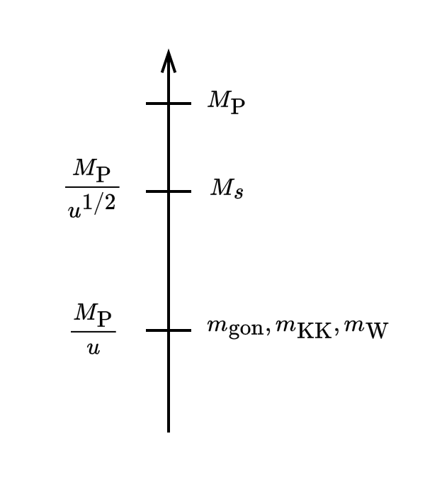
Figure 3: Structure of scales in the toy example in the text.

2.2.2 Difficulties for a single large dimension or more than two

In the above $s,u^{(2)}\rightarrow\infty$ limit two dimensions become large. An interesting question is how things change if only one dimension is large. One can see that this is obtained in the limit $s,u^{(2)},t^{(2)}\sim u$, $u\rightarrow\infty$, as explained in appendix A. Then the winding states remain at the string scale and only the KK tower becomes light. This however turns out to be problematic for the following reason. All Yukawa couplings in the theory get an overall prefactor ${\rm Vol}_{X}^{-1/2}$. Thus in a theory containing the SM in the limit $t^{(2)}\rightarrow\infty$ the Yukawas of all SM particles will get suppressed, and not only those of neutrinos. We know however that there are Yukawa couplings of order one, like that of the top quark, so that this limit is inconsistent with observation.

Notice that this unwanted suppression is there irrespective of what the origin of tiny neutrino masses is. Thus a single large dimension implies in general too small Yukawa couplings. This is certainly true in the toroidal case. One may argue that in a general CY setting this need not be the case since in principle one can have that ${\rm Vol}_{X}$ remains unchanged even when a specific Kähler modulus grows to infinity. However, as we discuss in appendix A, this is only possible at the cost of some other Kähler modulus getting small. Then D2-branes wrapping a two-cycle whose area is controlled by this modulus will give rise to a light tower of particles, which will then open an additional dimension so that actually we no longer are in a single tower regime. Alternatively one could have D4-branes wrapping a shrinking four-cycle that generate a light tower with an analogous effect. Similar considerations can be drawn whenever one considers setups with an odd number of large dimensions. The reader interested in more details about the case with odd extra dimensions may consult appendix A.

Finally, one may consider limits in which four or six dimensions become large. This possibility does not imply having suppressed SM Yukawa couplings but, as discussed in appendix A, when applied to scenarios with small Dirac neutrino masses like the one in section 3, it gives rise to a quantum gravity cut-off that is ruled out experimentally. Given these difficulties, in the rest of the paper we will focus on setups with two large geometric dimensions, as in the toy model above.

3 The SM at intersecting D6-branes

Let us start by considering the simplest structure of D6-brane intersections which can reproduce the SM spectrum, see e.g. [6, 7, 8, 9, 10, 11, 12] and references therein.

The minimal set of $D6$-branes would involve four stacks $a,b,c,d$ (and their orientifold images $a^{*},b^{*},c^{*},d^{*}$), with multiplicities $N_{a}=3,N_{b}=2,N_{c}=N_{d}=1$, so that the naive gauge group reads $U(3)_{a}\times U(2)_{b}\times U(1)_{c}\times U(1)_{d}$. Instead of $N_{b}=2$ one can also consider $N_{b}=1$ if both $D6_{b}$ and $D6_{b}^{*}$ coincide and give rise to the gauge group $USp(2)\simeq SU(2)$. Let us first look at this simpler class of models. The gauge group will be $SU(3)\times SU(2)\times U(1)_{a}\times U(1)_{c}\times U(1)_{d}$. Here $U(1)_{a}$ and $U(1)_{d}$ correspond to gauged baryon number and (minus) lepton number respectively, while $U(1)_{c}$ corresponds to the diagonal component of right-handed weak isospin. The hypercharge is a linear combination of the three $U(1)$’s, while the other two become massive, due to $B\wedge F$ couplings. At the intersection of D6-branes, i.e. at $X_{4}$ and a points in the compact space $X_{6}$, massless chiral multiplets appear. In particular, to have correct SM quantum numbers, the intersection numbers are given by [54, 42]

$$\begin{split}I_{ab}=I_{ab^{*}}=3\,,&\qquad I_{ac}=I_{ac^{*}}=-3\,,\\ I_{db}=I_{db^{*}}=-3\,,&\qquad I_{dc}=I_{dc^{*}}=3\,,\end{split}$$ (3.1)

with the rest of the intersection numbers vanishing. The hypercharge is given by the linear combination

$$Y\,=\,\frac{1}{6}Q_{a}-\frac{1}{2}Q_{c}+\frac{1}{2}Q_{d}\,,$$ (3.2)

whose gauge boson should remain massless (no $B\wedge F_{Y}$ couplings) in the spectrum. The reader may check that each of the SM fields at the intersections have the correct hypercharge assignment. There are in addition two other $U(1)$’s which in general will be massive. Note that the right-handed neutrinos are localised at the intersection of the branes $c$ and $d^{*}$, and are neutral under hypercharge, as they should.

As it stands this simple configuration is not appropriate for our purposes for two reasons. Indeed, as we described in the previous section and in [17], in order to get tiny Yukawa couplings for the neutrinos, at least one of the gauge couplings $g_{c}$ or $g_{d}$ must be very small, corresponding to either the D6-branes $c$ or $d$ wrapping a three-cycle with large volume. However, then the hypercharge coupling $g_{Y}$ will also go to zero, which is incompatible with its experimental value $g_{Y}\simeq{\cal O}(0.3)$. Also, the charged leptons live at the $cd$ intersection and will also get a tiny Yukawa coupling, against the experimental results. Thus the desired brane configuration should differentiate between charged leptons and the right-handed neutrino sector.

A simple generalisation of this D-brane configuration that does the job can be obtained by adding an extra brane ${\tilde{c}}$ and also not imposing the condition $b=b^{*}$ on the electro-weak brane $b$. In fact, for simplicity, we will consider a D-brane configuration that is fully separated from its orientifold images and the orientifold planes, in the sense that all intersection numbers of the form $I_{ab*}$ and $I_{a{\rm O6}}$ vanish. In mirror type IIB setups, this feature is easily implemented by considering D3-branes at singularities away from the orientifold planes possibly with flavour D7-branes [55]. In the type IIA framework one should be able to engineer them via embedding the local models of [56] into global CY orientifold compactifications. We do not claim that this is the unique way to build SM brane configurations with small Dirac neutrino masses, but this mirror picture provides us with an explicit framework, sufficient for the purpose of showing the minimal ingredients required to obtain the result. In appendix B, an $SU(5)$ configuration is also displayed in which the same structure to obtain small neutrino Yukawa couplings is shown.

So let us consider a brane configuration with stacks $a,b,c,{\tilde{c}},d$ and intersection pattern described as in table 2.

Intersection	Matter fields	Charge	$Q_{a}$	$Q_{b}$	$Q_{c}$	$Q_{\tilde{c}}$	$Q_{d}$	$Y$	$Q_{\nu}$
$(ab)$	$Q_{L}$	$(3,2)$	1	-1	0	$0$	$0$	1/6	0
$(a{\tilde{c}})$	$U_{R}$	$({\bar{3}},1)$	-1	0	0	$1$	$0$	-2/3	1
$(ac)$	$D_{R}$	$({\bar{3}},1)$	-1	0	1	$0$	$0$	1/3	0
$(bd)$	$L$	$(1,2)$	0	-1	0	$0$	$1$	-1/2	-1
$(cd)$	$E_{R}$	$(1,1)$	0	0	1	$0$	$-1$	1	1
$({\tilde{c}}d)$	$\nu_{R}$	$(1,1)$	0	0	0	$1$	$-1$	0	2
$(b{\tilde{c}})$	$H_{u}$	$(1,1)$	0	1	0	$-1$	$0$	1/2	-1
$(bc)$	$H_{d}$	$(1,1)$	0	1	-1	$0$	$0$	-1/2	0

Table 2: SM spectrum and D-brane $U(1)$ charges in the configuration with an five branes (3.3). The intersection numbers for the Quark-Lepton sector are $I_{ab}=-I_{ac}=-I_{a\tilde{c}}=-I_{bd}=I_{cd}=I_{\tilde{c}d}=3$, and for the Higgs sector $I_{bc}=I_{b\tilde{c}}=6$.

D-brane configurations with similar structure have been considered previously in e.g.[18, 57, 58]. The gauge group is of the form

$$SU(3)\times SU(2)\times U(1)_{a}\times U(1)_{b}\times U(1)_{c}\times U(1)_{\tilde{c}}\times U(1)_{d}\,.$$ (3.3)

Most $U(1)$’s here are anomalous and will get a mass via $B\wedge F$ couplings implementing a Stückelberg mechanism. The hypercharge is now identified with

$$Y\,=\,\frac{2}{3}Q_{a}+\frac{1}{2}Q_{b}+Q_{c}\,,$$ (3.4)

and it should be free of Stückelberg couplings to axions. In appendix C we describe the $U(1)$ anomaly structure of this setting and the general conditions that should be obeyed in a specific CY orientifold so that all $U(1)$’s but hypercharge become massive and the $U(1)_{\tilde{c}}$, $U(1)_{d}$ couplings may become small. Figure 4 symbolically summarises the intersections which are assumed. In the figure, any closed triangle corresponds to a Yukawa coupling allowed by the $U(1)$ charges.

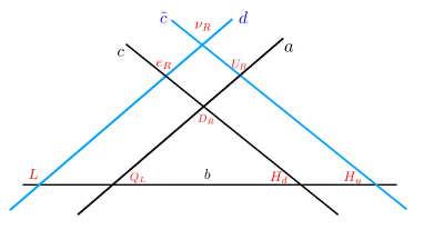
Figure 4: Scheme of the intersections in the SM-like quiver of table 2. The branes ${\tilde{c}},d$ in blue wrap a large volume, leading to suppressed Yukawa couplings for the right-handed neutrinos.

Note that the simpler configuration in (3.1) is recovered if we identify the branes ${\tilde{c}}$ with $c^{*}$ and replace the $U(2)$ of brane $b$ by an $USp(2)$. The essential new ingredient that the present configuration brings is that now the right-handed neutrinos are localised at the intersection of branes ${\tilde{c}}$ and $d$ whose associated $U(1)$’s do not appear in the expression for the hypercharge. Thus their associated gauge couplings $g_{\tilde{c}},g_{d}$ may tend to zero without affecting any of the SM gauge couplings.

Let us use the type IIB mirror picture of D-branes at singularities to illustrate how all the features described above can be achieved in a single construction. Let us first assume that the D-branes $a$, $b$, $c$ correspond to D3-branes at a singularity away from the orientifold, that reproduces the chiral content of this subsector. From here it follows that (3.4) is free of any $B\wedge F$ coupling and hence massless. The branes $\tilde{c}$ and $d$ are instead assumed to be flavour D7-branes. This will generically imply that all additional anomaly-free $U(1)$’s that arise from (3.3) develop $B\wedge F$ couplings. Moreover, it will imply that all the SM Yukawas involve an ${\cal N}=2$ sector and are insensitive to the bulk moduli, except those that involve right-handed neutrinos. Indeed, the $\nu_{R}$ arise at the intersection of two flavour D7-branes and far away from the singularity. As such, their gonion spectrum will be sensitive to the CY bulk moduli, and so will be their Yukawas.

3.1 The neutrino Yukawa coupling

Let us now consider the Yukawa coupling for the neutrinos:

$${\cal L}_{\nu}\,=\,Y_{\nu,ij}\,H_{u}L^{i}\nu_{R}^{j}\,.$$ (3.5)

Dirac neutrino masses arise when the Higgs field $H_{u}$ acquires a vev, and we want to study the conditions under which these masses become small, of order $(10^{-1}-10^{-4})$ eV. As we described in the last section, in limits of large complex structure a small Yukawa is accompanied with a light gonion tower. In our setup, one expects that only the sector $\tilde{c}d$ has light gonions, since it corresponds to the intersection of the two ‘flavour’ branes. Moreover, it was argued in [17] that when a gonion tower at the intersection $\tilde{c}d$ asymptotes to zero mass in Planck units, at least one of the gauge couplings $g_{\tilde{c}},g_{d}$ also goes to zero. In other words, we have that the imaginary part of the complex structure field

$$U\equiv\left(P_{\tilde{c},K}+P_{d,K}\right)U^{K}\,,$$ (3.6)

tends to infinity, since

$$u\equiv\mbox{Im}\,U=\frac{2\pi}{g_{\tilde{c}}^{2}}+\frac{2\pi}{g_{d}^{2}}\,.$$ (3.7)

The limits of interest will thus be those in which $u\to\infty$ and the rest of the gauge couplings $g_{a}$, $g_{b}$ and $g_{c}$ remain constant, so that the hypercharge coupling is unaffected along the limit.

The complex structure saxion (3.7) can be interpreted as the gauge coupling of the gauge group $U(1)_{\nu}$ felt by the right-handed neutrinos, which corresponds to the combination coupling to the generator

$$Q_{\nu}\,\equiv\,Q_{\tilde{c}}-Q_{d}\,,$$ (3.8)

so that $Q_{\nu}(\nu_{R}^{i})=2$. This gauge group will be anomalous (see appendix C) and hence should be massive due to a $B\wedge F$ coupling of the form

$$S_{BF_{\nu}}\,=\,Q_{\nu}^{K}\,B_{K}\wedge F_{\nu}\,\equiv\,\left(Q_{\tilde{c}}^{K}-Q_{d}^{K}\right)\,B_{K}\wedge F_{\nu}\,,$$ (3.9)

where the $2Q_{\tilde{c},d}^{K}$ are integers determined by the wrapping numbers of the D6-branes $\tilde{c}$ and $d$, respectively, that represent the above $U(1)$ generators, see [17] and the discussion of section 2 for their precise definition. The coupling (3.9) determines the way in which the chiral multiplet associated to $U$ and the vector multiplet $V_{\nu}$ that corresponds to (3.8) combine in the Kähler potential $K$. In particular, the Green–Schwarz mechanism fixes that these two multiplets appear in the combination $M_{\rm P}^{-2}K=k\left(u-I_{\tilde{c}d}V_{\nu},\dots\right)$, where $k$ is a real function of $u$ and other complex structure saxions. In the regime in which $u\to\infty$ we can approximate this function as

$$M_{\rm P}^{-2}K\,\simeq\,-\,n\log(u-I_{\tilde{c}d}V_{\nu})-\log(g(\{u^{I}\}))+\dots\,,$$ (3.10)

where $1\leq n\leq 4$, $g$ is a polynomial on a subset $\{u^{I}\}$ of the complex structure saxions $\{u^{K}\}$ and the dots represent subdominant terms of the Kähler potential in this regime. Along this limit the kinetic term for (3.8) behaves as

$$\mbox{Re}\,f_{\nu}\,\simeq\,u\implies g_{\nu}\,\sim\frac{1}{u^{1/2}}\to 0\,.$$ (3.11)

Additionally, associated to the $B\wedge F$ coupling (3.9) there is an FI-term that reads

$$\xi_{\nu}\simeq Q_{\nu}^{K}\ell_{K}\,M_{\rm P}^{2}\,.$$ (3.12)

If all the indices $K$ that appear in this expansion are contained in the subset of complex structure saxions $\{u,u^{I}\}$ that appear in the leading term of the Kähler potential (3.10), then one can show that $\ell_{\rm min}\simeq 1/u$, where $\ell_{\rm min}$ is defined as in (2.7). Then, applying such an estimate, one obtains that

$$m_{{\rm gon},\nu}\,\sim\,\frac{M_{\rm P}}{u}\,\sim\,g_{\nu}^{2}M_{\rm P}\,.$$ (3.13)

Let us consider the scaling of the Yukawa coupling in the large $u$ limit. As described in section 2 in principle one gets the structure

$$Y_{\nu,ij}\,\simeq\,e^{-\phi_{4}}\left(\frac{m_{{\rm gon},\nu}^{i}}{M_{\rm P}}\right)^{1/2}\left(\frac{m_{{\rm gon},L}^{j}}{M_{\rm P}}\right)^{1/2}\left(\frac{m_{{\rm gon},H_{u}}}{M_{\rm P}}\right)^{1/2}\,.$$ (3.14)

However, if we follow our mirror type IIB intuition in which the branes $a$, $b$, $c$ are represented by D3-branes at a singularity and $\tilde{c}$, $d$ are ‘flavour’ D7-branes, we only expect the angles at the intersection $\tilde{c}d$ to be directly sensitive to the bulk modulus $u$, and so $m_{{\rm gon},\nu}$ to be the lightest tower. The other towers will be less relevant for determining the asymptotic behaviour of the Yukawa, although they may play a role in the details of the flavour dependence (along with the holomorphic Kähler dependent factor $W_{ijk}$). For the heaviest neutrino generation (which we take as the 3^rd one) one expects $m_{{\rm gon},L}^{3{\rm rd}}\simeq m_{{\rm gon},H_{u}}\simeq M_{s}\simeq e^{\phi_{4}}M_{\rm P}$, so that one gets

$$Y_{\nu,3}\,\simeq\,\left(\frac{m_{{\rm gon},\nu}^{i}}{M_{\rm P}}\right)^{1/2}\,\simeq\,g_{\nu}\,.$$ (3.15)

This is a remarkably simple result, which allows us to fix all the relevant mass scales in the theory, as we describe below. Many of the features of our scenario reproduce those in the toy model of section 2.2.1, because physical Yukawa couplings are, to leading order, only sensitive to the local geometry around D-brane intersections. Notice that the main ingredient of this construction is a field trajectory of infinite distance that leaves the hypercharge coupling invariant but sends $g_{\nu}\to 0$. Thus we believe that is a general result which should apply to most SM-like D-brane in type II CY orientifolds, whenever hierarchically small Dirac Yukawa couplings for neutrinos is pursued.

Note that this behaviour of the Yukawa coupling may be traced back to the fact that the field metric $K_{\nu}^{i}$ (in units of $M_{s}$, see [17] for details) for the right-handed neutrinos at the intersections becomes singular as the $\nu_{R}$ gonions become light, i.e.

$$K_{\nu}^{i}\,\simeq\,\frac{M_{\rm P}}{m_{{\rm gon},\nu}^{i}}\,\sim\,u\,.$$ (3.16)

From the supergravity equation for canonically normalised Yukawas

$$Y_{ijk}\ =\ {W}_{ijk}\,\,e^{K/2}\left(K_{i}K_{j}K_{k}\right)^{-1/2}\ ,$$ (3.17)

the behaviour $Y_{\nu}\sim K_{\nu}^{-1/2}\sim u^{-1/2}$ is inherited.

While neutrino Yukawa couplings behave like $Y_{\nu}\sim u^{-1/2}$, and produce tiny Dirac neutrino masses, one may wonder whether large right-handed Majorana masses could also be present at the same time. They could in principle be generated by charged D-brane instantons, as mentioned in the introduction. This would be bad news, because the resulting neutrino masses would be too small. However, due to the constraints on the intersection numbers of such D-brane instantons with the SM branes [13], one expects that the instanton action depends on the field $U$. From where one obtains a Majorana mass suppression of order $e^{-u}$ which deactivates the see-saw mechanism.

The species scale

One of the results of [17] is that when some gonion towers become light, some dimensions of the compactification manifold become large. As already mentioned, the case with a single large extra dimension is in tension with light gonion towers, so let us consider that two internal dimensions become large along the limit $u\to\infty$ just like in the toy example of section 2.2.1. These two towers of KK/winding states have masses of the same order as the gonions: $m_{{\rm KK}}\sim m_{{\rm w}}\sim M_{\rm P}/u$. In addition there can be KK-like towers coming from open strings at the worldvolume of the D6${}_{\tilde{c}}$ and/or D6_d branes, also with masses of this order.

Along this complex structure limit the string scale also falls polynomially with $u$. One way to estimate its scale is to think that since we are probing infinite distance limits with open string states, one would expect the string scale to be the quantum gravity cut-off of the theory. In fact, this expectation agrees in toroidal models, where the quantum gravity cut-off is computed in different instances (see [17, section 5]). The quantum gravity cut-off, oftentimes dubbed the species scale [60, 61, 62], is the scale that emerges for a large number of species well below the Planck scale and where the effects of quantum gravity are not innocuous. It may be defined in several ways, and its value is of order

$$\Lambda_{\rm QG}\simeq\frac{M_{\rm P}^{D}}{N^{1/(D-2)}},$$ (3.18)

with $D$ the number of spacetime dimensions and $N$ the number of fields below $\Lambda_{\rm QG}$. For the case at hand, the number of species is given by $\Lambda_{\rm QG}^{2}\simeq\,N\,m_{{\rm light}}^{2}$, and after substituting into equation (3.18) we arrive at

$$\Lambda_{\rm QG}\simeq M_{s}\simeq\frac{M_{\rm P}}{u^{1/2}}\ \simeq\ g_{\nu}M_{\rm P}\,.$$ (3.19)

So all in all the structure of scales is again as in figure 3. At the lowest scale with a mass $\sim g_{\nu}^{2}M_{\rm P}$ there is the tower of $\nu_{R}$-like gonions, KK/winding states of two extra dimensions, and the corresponding KK/winding states of the bulk of the large branes D6${}_{\tilde{c}}$ and D6_d. Then the string scale is located at the geometric mean of that scale and the Planck scale: $M_{s}\simeq g_{\nu}M_{\rm P}$.

Finally, one can apply the same analysis to limits with four or six large dimensions, as performed in appendix A. There one finds that the relation becomes $\Lambda_{\rm QG}\sim g_{\nu}^{\frac{2p}{p+2}}M_{\rm P}$, where $p$ is the number of large dimensions. When combined with (3.15) and the experimental data for neutrino masses, this gives an unacceptably low species scale.

3.2 The light vector boson mass

An important point to address is to determine the mass of the massive boson $V_{\nu}$ that couples to the right-handed neutrinos. The point is that extra massive $U(1)$ bosons beyond hypercharge are generally given a mass that is essentially determined by the size of their FI terms. So most of these $U(1)$ will have masses on the order of the string scale, if their FI terms do not depend on $u$. However, in our setup such a dependence is expected, given the presence of gauge couplings in (2.5), and in particular of $g_{\nu}\sim u^{-1/2}$. Because from the Kähler potential we will also have some kinetic terms that scale as $G_{uu}\sim u^{-2}$, in principle one could have a Stückelberg mass for $V_{\nu}$ that scales as $M_{V_{\nu}}\sim g_{\nu}^{3}M_{\rm P}$. Such a gauge boson would then be the lightest massive particle in the spectrum. With $g_{\nu}\simeq Y_{\nu}$, that would correspond to a vector boson with a mass $M_{V_{\nu}}\simeq 10^{-9}$eV and a coupling $g_{\nu}\simeq 10^{-12}$, which would be already ruled out by experiments measuring deviations of Newton’s laws at short distances.

In fact there are several contributions to the mass of this vector boson, which makes it typically much heavier. First, there is a model independent lower limit for its mass

$$M_{V_{\nu}}\,\gtrsim\,m_{\nu,3}\,\simeq\,0.1\,{\rm eV}\,,$$ (3.20)

which comes from the fact that the Higgs boson $H_{u}$ is charged under $Q_{\nu}$. Once the Higgs gets a vev the vector boson gets a contribution $\delta(M_{V_{\nu}}(\text{Higgs}))\simeq g_{\nu}|\langle H_{u}\rangle|\simeq m_{\nu,3}$. Another possible, but model dependent contribution may arise if some right-handed sneutrino gets a vev. Then one would get $\delta(M_{V_{\nu}}(\text{sneutrino}))\simeq g_{\nu}|\langle\nu_{R}^{i}\rangle|\lesssim g_{\nu}M_{s}$. This would be of the order of the $\nu_{R}$-gonion tower.

Finally, in general there are additional contributions to $M_{V_{\nu}}$ that come from (2.5), besides the one that we have already accounted for. These come from considering that the vector $Q^{K}_{\nu}$ is not proportional to the field direction $U$ defined in (3.6). To be more concrete, let us in particular consider that $Q^{K}_{\nu}$ has entries pointing along some of the fields $u^{I}$ that appear in (3.10), that do not grow along the limit. Then the total Stükelberg mass for the gauge boson $V_{\nu}$ will be of the form

$$M_{V_{\nu}}\,\simeq\,g_{\nu}^{2}M_{\rm P}^{2}\left(\frac{I_{\tilde{c}d}^{2}}{u^{2}}+4G_{IJ}Q^{I}_{\nu}Q^{J}_{\nu}\right)\,,$$ (3.21)

where $G_{IJ}=-\frac{1}{2}\partial_{u^{I}}\partial_{u^{J}}\log g(\{u^{I}\})$ is a homogeneous function of degree minus two the on the fields $u^{I}$, thus independent of $u$. In the limit $u\gg u^{I}$ we can take $G_{IJ}Q^{I}_{\nu}Q^{J}_{\nu}$ to be an order one numeric factor, and so the mass of the vector boson is of order $M_{V_{\nu}}\simeq g_{\nu}M_{\rm P}\simeq M_{s}$, namely of order the string scale. Note that this is precisely what happens in the toy model of section 2.2.1, where the vector $Q_{a}^{K}$ corresponding to the brane $a$ has non-vanishing entries along all fields, from where (2.20) follows. Of course one can still get a light vector boson by considering a more involved limit in which all the $u^{I}$ that couple to $Q^{I}_{\nu}$ go to infinity. However, then typically one obtains that other gauge couplings (like SM couplings) would also get very small.

To sum up, the Stückelberg mass of the vector boson in $V_{\nu}$ is quite model dependent, in the sense that is quite sensitive to the integer entries $2Q_{\nu}^{I}$ of the D-brane model. In terms of the 4d EFT, what these integers specify is the field dependence of the FI-term associated to $V_{\nu}$. In general, one can only state that the $U(1)_{\nu}$ gauge boson may have a mass in the region

$$m_{\nu,3}\,\lesssim\,M_{V_{\nu}}\,\lesssim\,g_{\nu}M_{\rm P}\,\simeq\,M_{s}\,,$$ (3.22)

with the largest values being more generic. In the low range of masses the vector boson mass is strongly constrained experimentally, as we briefly discuss below.

4 Dirac neutrino masses: all scales fixed

From the previous discussions it is clear that in our setup all scales appearing in the theory are determined by a single parameter $g_{\nu}$. Luckily, we can draw information about its value from experimental information on neutrino masses and mixings. To make an estimate let us assume normal hierarchy of neutrino masses. Similar results would be obtained for an inverted hierarchy. Let us recall from (2.8) and (2.9) that the complete Yukawa couplings of neutrinos ${\tilde{Y}}_{\nu}$ (including now for completeness the dependence on the Kähler moduli) will have the form

$${\tilde{Y}}_{\nu,i}\,\simeq\,Y_{\nu,i}\,\delta^{i}\,,\qquad i=1,2,3\,,$$ (4.1)

where we have taken diagonal Yukawas for simplicity. Also, $\delta^{i}$ may be flavour dependent constants, analogous to those for charged lepton-fermion matrices, which are expected to give tiny corrections compared to the leading factor of $Y_{\nu,i}$ discussed in the last section. Let us consider two limiting possibilities:

i) Universal $\nu_{R}$ gonion towers

In toroidal examples and in general compactifications without strong local curvature effects, one expects $Y_{\nu,i}=Y_{\nu}$, which corresponds to the three neutrino intersections having their corresponding gonion masses at the same scale (equal angles). In this case for the heaviest third generation neutrino one expects $\delta\simeq 1$, so one has

$${\tilde{Y}}_{\nu,3}\,\simeq\,Y_{\nu}\,g_{\nu}\,,\qquad i=1,2,3\,,$$ (4.2)

as already discussed in the previous section. Moreover, for the third (heaviest) neutrino generation one has

$$m_{\nu,3}\,=\,Y_{\nu,3}\langle|{H_{u}}|\rangle\,.$$ (4.3)

Then, the mass of the heaviest neutrino can be estimated from the neutrino oscillation data, i.e. $m_{\nu,3}\simeq\sqrt{\Delta m_{32}^{2}}\simeq 5\times 10^{-2}$ eV. From here one obtains

$$Y_{\nu,3}\,\simeq\,g_{\nu}\,\simeq 7\times 10^{-13}\,.$$ (4.4)

Using this value for the gauge coupling $g_{\nu}$, one can then calculate the different numerical scales that arise, which are shown in table 3.

String Scale	SM gonions	$\nu_{R}$ tower	large dim	Vector boson	Gravitino
$M_{s}$	$m_{\rm gon}^{\rm SM}$	$m_{\rm gon}^{\nu}$	$m_{\rm{KK/w}}$	$M_{V_{\nu}}$	$m_{3/2}$
$g_{\nu}M_{\rm P}$	$\lesssim M_{s}$	$g_{\nu}^{2}M_{\rm P}$	$g_{\nu}^{2}M_{\rm P}$	$g_{\nu}|{\bar{H}}|-g_{\nu}M_{\rm P}$	$\lesssim M_{s}^{2}/M_{\rm P}$
$g_{\nu}=Y_{\nu,3}$ ,  700 TeV	$\lesssim 700$ TeV	$500$ eV	$500$ eV	$0.5$ eV- $700\$TeV	$\lesssim\ 500$ eV
$g_{\nu}=Y_{\nu,1}$ ,  10 TeV	$\lesssim 10$ TeV	$0.1$ eV	$0.1$ eV	$10^{-3}$ eV- $10\$TeV	$\lesssim\ 0.1$ eV

Table 3: Spectrum of masses and scales from imposing Dirac character to neutrino masses in string theory. Numerical results are shown for two limiting cases with $g_{\nu}\simeq Y_{\nu,3}\simeq 7\times 10^{-13}$ and $g_{\nu}\simeq Y_{\nu,1}\simeq 10^{-14}$.

ii) Non-universal $\nu_{R}$ gonion towers

Another possibility is that the local intersection angles of the three generations are not universal so that the angle of the lightest generation $\nu_{R}$ is $\theta^{1}\ll\theta^{2,3}$. This may happen when the D6-brane intersection are around regions of $X_{6}$ with strong curvature, breaking universality. As a limiting case, we may consider the situation in which the lightest generation got its smallest Yukawa coupling from $Y_{\nu,1}$ (i.e. $\delta^{1}=1$). In that case one has

$$Y_{\nu,1}\,\simeq\,g_{\nu}\,.$$ (4.5)

The mass of the lightest neutrino is experimentally unknown. Cosmological bounds suggest [64, 65] that $m_{\nu,1}\lesssim 20-40\times 10^{-3}$ eV and the bounds based on Swampland arguments mentioned below yield $m_{\nu,1}\lesssim 7\times 10^{-3}$ eV [27, 29, 28]. We show the numerical results in this case assuming for comparison $m_{\nu,1}\simeq 1\times 10^{-3}$ eV. We then have $g_{\nu}\simeq Y_{\nu,1}\simeq 10^{-14}$. The corresponding structure scales is shown in table 3.

Let us comment on the different masses at the different scales.

• $M_{s}\simeq g_{\nu}M_{\rm P}\simeq 10-700$ TeV. This is the string scale, which is the fundamental scale of the theory.

• $m_{\rm gon}^{\rm SM}\simeq m_{\rm KK}^{\rm D6}\simeq m_{\rm KK}\ \lesssim g_{\nu}M_{\rm P}\simeq 10-700$TeV. Below the string scale there are several types of particles: 1) There are the gonions and vector-like copies of the SM fermions, which are expected to be below $M_{s}$. In fact, eventually SUSY has to be broken, so squarks and sleptons may be considered as particularly light gonions. 2) There are KK copies of the SM gauge bosons and their gaugini. Again, after SUSY breaking there will also be the gauginos of the SUSY SM. 3) In general there will be additional massive $U(1)$’s, like those that are anomalous but not suppressed, with masses in this region. 4) The graviton KK copies corresponding to four (not so large) dimensions.

• $m_{\rm gon}^{\nu_{R}}\simeq m_{\rm KK/w}^{\rm large}\simeq m_{\rm KK/w}^{Q_{\nu}}\simeq g_{\nu}^{2}M_{\rm P}\simeq 0.1-500$ eV. At this scale there are three types of particles again: 1) The gonion tower with copies of right-handed neutrinos. They come along with their sneutrinos if SUSY-breaking is not felt strongly by this sector; 2) The KK/w copies of the gauge boson which couples to $Q_{\nu}$, and its gaugini; 3) The KK/w towers of the two large dimensions.

• $M_{V_{\nu}}\simeq 10^{-3}-0.1\ {\rm eV}$  to  $10-700\$TeV. The vector boson associated to the generator $Q_{\nu}$ may be the lightest new particle in the setting (along with its gaugino). As we said the vector gets a tiny model-independent Stückelberg mass of order $g_{\nu}^{3}$ eV. However there is the Higgs boson contribution to the mass which is of order neutrino masses. Furthermore, if additional Stükelberg couplings to $Q_{\nu}$ exist, the vector boson may be as massive as the string scale $\sim 10-700$ TeV.

• $m_{3/2}\lesssim g_{\nu}^{2}M_{\rm P}$. Since the fundamental cut-off is at the string scale $M_{s}\simeq g_{\nu}M_{\rm P}$, the gravitino mass is expected to have a mass $m_{3/2}\lesssim M_{s}^{2}/M_{\rm P}\simeq g_{\nu}^{2}M_{\rm P}\simeq 0.1-500$ eV. Note that then supergravity mediated SUSY breaking mass terms will be tiny, of order $0.1-500$ eV, and hence they cannot be the leading source of SUSY breaking in the SM sector.

To this novel spectrum beyond the SM one has to add the modulus $U$ itself, whose vev determines all hierarchies. One expects that some dynamics fixes its value at $u\simeq g_{\nu}^{-2}$. In particular, it is conceivable that the above mentioned tiny soft terms from supergravity mediation could induce a mass of order $0.1-500$ eV for this modulus. We will not consider here the possible mechanisms that could give rise to this modulus stabilisation, nor the stabilisation of the other four compact dimensions.

4.1 Some phenomenological consequences and constraints

In this section we just give a preliminary overview of the possible observable consequences of such a spectrum. An incomplete list includes:

• Constraints on the vector boson mass/coupling: There are experimental limits in the plane gauge-coupling versus mass for ‘dark photon’ $U(1)$’s beyond the standard model. They mostly arise from astrophysical constraints coming from over-cooling of stars, mainly the Sun, red giants, and horizontal branch stars, see e.g.[66, 67] for a recent discussion and references. There are also constraints from fifth-forces. Thus e.g. in those references constraints for a vector boson coupled to $(B-L)$ are presented. They find that e.g. a gauge coupling $g_{B-L}\simeq 10^{-12}-10^{-13}$ and a mass $M_{B-L}\simeq 1$ eV are barely consistent with the bounds. It would be interesting to make a similar analysis with the gauge group which couples to our generator $Q_{\nu}$. The latter is not orthogonal to $U(1)_{B-L}$ so we would expect similar limits in the coupling/mass plane. Thus the presence of this model-independent ‘dark photon’ in the theory may provide interesting experimental constraints.

• Constraints on KK and string scales: There are experimental constraints on the number and size of extra dimensions (see [68] for a recent review and references). In our case we have two large dimensions with a scale $\sim 1/(500\ {\rm eV})$, while the other four are of the order of the string scale $1/M_{s}$. Tests of the gravitational force at sub-millimeter scales give the bound $M_{s}\geq 4.0$ TeV [69]. Searches of string resonances in ATLAS and CMS at LHC give a bound $M_{s}\gtrsim 8$ TeV. There are stronger astrophysical limits under the assumption that the KK states decay with a substantial branching ratio to photons, but that is not the case for the two large dimensions in question, which are isolated from SM couplings.

  These limits are below $M_{s}\simeq 10-700$ TeV which we have in the Dirac neutrino setting here described, but close to possible tests at LHC and future colliders. There are also constraints on KK SM gauge bosons, of order a few TeV.

• Neutrino masses

  The most obvious prediction is the Dirac character of neutrinos. Another interesting aspect is the mixing of neutrinos with the neutralinos of the $U(1)_{\nu}$ gauge boson. Indeed, if right-handed sneutrinos get a vev $\langle{\tilde{\nu}}_{R}\rangle=v\leq M_{s}$, the right-handed neutrinos get a mixing mass term of order $\lesssim g_{Q_{\nu}}M_{s}\simeq 0.1-500$ eV with the $U(1)$ gaugino. Thus the gaugino may be present as a ‘sterile neutrino’ which could play a role in neutrino oscillation physics.

The above is just a partial list of phenomenological implications. Thus one expects the presence of gonion copies of the SM quarks and leptons which would be below the string scale $M_{s}\simeq 700$ TeV. Some gonions, which would look like vector-like partners of quarks and leptons, could have masses around a few TeV. In addition, once SUSY is broken, the SUSY partners of the SM would be expected below the gonion scale. Thus there could be a plethora of new particles above LHC scales, possibly within FCC reach, if some of the particles remain light as in the ‘mini-split’ scenario of [70, 71, 72] in which a large SUSY breaking scale up to $\sim 10^{3}$ TeV is considered. Also, $\nu_{R}$ gonions or lightest KK particles could be candidates for dark matter. We leave these possible phenomenological implications to future research.

Challenges

An important question is that of baryon stability. Indeed with a fundamental scale as low as $M_{s}\simeq 10^{6}$ GeV, there is a danger of too fast baryon decay: In a SUSY setting the most dangerous operators are those of dimension 4 which violate R-parity in the superpotential, $(Q_{L}D_{R}L),(U_{R}D_{R}D_{R}),(LLE_{R})$. Those are all forbidden by the $U(1)_{\nu}$ symmetry, as well as the dimension 5 operators $(Q_{L}Q_{L}Q_{L}L)$ and $(U_{R}U_{R}D_{R}E_{R})$. One can also check that the standard $6d$ operators of baryon decay appearing in GUT’s are also forbidden. It would be interesting to check whether this suppression may be sufficient to ensure baryon stability in a setting like this, once one includes operators of even higher dimensions.

There is another challenge present in this particular setting, which is that ‘$\mu$-term’ bilinears $\mu H_{u}H_{d}$ are also forbidden by the $U(1)_{\nu}$ symmetry. Although not as crucial as baryon stability, the absence of such a term may be problematic for the Higgs and Higgsino sectors of SUSY theories, since then $H_{u}$ and $H_{d}$ may not align when getting a vev. In fact a $\mu$-term may in principle be induced at the non-perturbative level from charged instantons, along the lines of refs. [13, 14, 15, 16, 48, 49, 50, 51]. In the present case the existence of Euclidean instantons with charges under $U(1)_{b}\times U(1)_{c}\times U(1)_{\tilde{c}}$ would be required. Checking whether the required instantons exist would require a fully-fledged string compactification. We do not think that this specific $\mu$-problem is generic for any possible semirealistic brane configuration leading to small neutrino Yukawas. An example of this is the $SU(5)$ model described in appendix B. There a $\mu$-term is allowed, not forbidden by any symmetry and still one can obtain suppressed neutrino Yukawa couplings in a way similar to the one considered in the above SM-like configuration.

5 The cosmological constant and Swampland constraints

In the previous sections we have not considered any input from Swampland criteria [73, 74]. Briefly speaking, the Swampland Programme (see [21, 22, 23, 24] for reviews) attempts to identify the general patterns that an EFT must obey so that it may be part of a consistent theory of Quantum Gravity (QG). One of the best tested Swampland conjectures is the Weak Gravity Conjecture [74], which states that in any $U(1)$ theory coupled to QG there must exist a particle of charge $q$ with mass obeying $m\leq\sqrt{2}qgM_{\rm P}$. In the present case the tower of gonions satisfies this condition. In addition, the Swampland distance conjecture [75] (SDC) states that as we move in moduli space at infinite distance a tower of states must become massless. In the setting discussed in this paper, at large $u\rightarrow\infty$ towers of gonions and KK/winding states appear.

Other classes of Swampland conditions depend on the structure of the vacua of scalar potentials. These other hypotheses have not been tested at the same level as the WGC or the SDC but their implications may be quite important and their validity should be considered seriously. In this section we want to briefly describe some implications of this class of constraints as applied to our Dirac neutrino setting.

The AdS instability conjecture [25, 26] states that there are no consistent stable (non-SUSY) Anti-de-Sitter (AdS) vacua in string theory. This does not sound very useful since the observed universe seems to have positive cosmological constant rather than negative. Still it has been observed [76] that upon compactification of the SM on a circle AdS vacua appear unless the lightest neutrino mass 1) is Dirac and 2) is sufficiently light, in particular (see [27, 29, 28] for details) one finds that it must satisfy

$$m_{\nu,1}\,\leq a\,\Lambda_{{\rm cc}}^{1/4}\,,$$ (5.1)

where $a$ is a computable number of order one and $\Lambda_{{\rm cc}}$ is the cosmological constant. The origin of this bound is that the Casimir energy in 3d has a positive contribution from this lightest neutrino which is enough to avoid AdS vacua to develop, if the above constraint is obeyed. This works for Dirac neutrinos, which carry 4 degrees of freedom, but not for Majorana which only have 2, not enough to overcome the 4 bosonic degrees of freedom from photon and graviton. This nicely fits with the scheme we are exploring in this paper where neutrinos have tiny Dirac masses. This nice connection between neutrino masses and the cosmological constant is lost if neutrinos are Majorana.

The neutrino mass for the first generation is given by $m_{\nu,1}=Y_{\nu,1}|\langle{H_{u}}\rangle|$. In our scheme, the Yukawa coupling of the first generation may be written as $Y_{\nu,1}=g_{\nu}\delta^{1}$. One can then write

$$g_{\nu}\delta^{1}|{H_{u}}|\,\lesssim\,\Lambda_{{\rm cc}}^{1/4}\,,$$ (5.2)

so one gets the bound on the gauge coupling

$$g_{\nu}\,\lesssim\,\frac{\Lambda_{{\rm cc}}^{1/4}}{\delta^{1}|{H_{u}}|}\,.$$ (5.3)

For fixed EW scale and cosmological constant, this implies a very small value for $g_{\nu}$ and therefore a very light tower of gonion and KK-like states, that result in two large dimensions. Moreover, because all neutrino masses are suppressed by $g_{\nu}$, this explains why Dirac neutrinos are so light. This is required for the lightest neutrino to be sufficiently light to obey the Swampland bound (5.1). One can also turn around the argument and write

$$|{H_{u}}|\ \lesssim\ \frac{\Lambda_{{\rm cc}}^{1/4}}{\delta^{1}g_{\nu}}\ .$$ (5.4)

This shows that the EW scale is bounded and stable and related to the value of the c.c. Plugging the values $\Lambda_{{\rm cc}}^{1/4}\simeq 10^{-12}$ GeV, $g_{\nu}\simeq 10^{-12}$ and e.g. $\delta^{1}\simeq 10^{-2}$ one would recover $|{H_{u}}|\lesssim 10^{2}$ GeV. In this sense this provides a solution to the EW instability (hierarchy) problem, as already pointed out in refs.[77, 27, 78, 79].

To sum up, from a Swampland viewpoint, a Dirac character for the neutrino is required to avoid the Swampland AdS instability conjecture. Additionally, the bound (5.1) relates the neutrino mass scale to the cosmological constant and, combined with our scheme, explains why two large dimensions are required to have the lightest neutrino sufficiently light (see also [79]).

6 Summary and outlook

In this paper we have studied under which conditions neutrino Yukawa couplings may become asymptotically small in the moduli space of SM-like string compactifications. This would give rise to tiny Dirac masses for neutrinos once the Higgs gets a vev, which may be compatible with neutrino oscillation data. To work out this study we have used as a laboratory type IIA CY orientifolds with D6-brane configurations yielding the chiral content of the SM at their intersections. We believe however that, given the extended network of dualities among 4d, ${\cal N}=1$ string vacua, our results are expected to be quite general. In order to perform this analysis we have made use of the recent results of [17], in which the general behaviour of Yukawa couplings at infinite distance in moduli space was explored within the context of type IIA CY orientifolds.

While we want to consider limits along which the neutrino Yukawas are rendered tiny, at the same time we have to ensure that the SM gauge coupling constants as well as the quark and charged lepton Yukawas do not get a strong suppression along them. This condition turns out to be extremely constraining. Essentially it requires that a large complex structure direction (say $u\rightarrow\infty$) should be taken so that two extra compact dimensions become large with a mass scale $\sim M_{\rm P}/u$. At the same time a tower of $\nu_{R}$-like states becomes also light around the same scale. The neutrino Yukawa couplings are of order $Y_{\nu}\simeq u^{-1/2}$, and one also has $Y_{\nu}\simeq g_{\nu}$, where $g_{\nu}$ is the gauge coupling of the $U(1)$ gauge symmetry coupling to right-handed neutrinos, which is thus very weak. Fixing the neutrino Yukawa couplings at values consistent with neutrino data gives a value $g_{\nu}\simeq 7\times 10^{-13}$ so that one finds a lowered string scale $M_{s}\simeq g_{\nu}M_{\rm P}\simeq 700$ TeV, and the $\nu_{R}$ tower and extra large dimensions at a scale $\simeq 500$ eV. If one allows for a lack of universality in the $\nu_{R}$ gonion towers, these scales may be substantially lowered down to $10$ TeV and $0.1$ eV respectively. Thus our scenario a priori does not exclude a string scale not far away from LHC limis ($\sim 8$ TeV).

We have also examined the case of a single large dimension within the context of type IIA CY orientifolds with SM content. We find that irrespective of the issue of neutrino masses, in such a case all Yukawa couplings (not only the neutrino ones) are suppressed, which would be inconsistent with experiment.

To sum up, we find that tiny Dirac neutrino masses may be obtained in string theory, by imposing a lowering of the string scale to values $M_{s}\lesssim 10-700$ TeV and the existence of two large dimensions at a scale with a factor $\sim 10^{4}$ heavier than that of neutrino masses. This is at variance to what happens in the case of Majorana neutrino masses which require a large string scale $M_{s}\gtrsim 10^{14}$ GeV. It is also interesting to remark that, as emphasized in section 5, the AdS instability conjecture applied to the 3d SM implies that neutrinos should be Dirac. The latter arguments also give an explanation for the proximity of the neutrino and the cosmological constant scales.

The case of Dirac neutrino masses may potentially lead to phenomenology much richer than the Majorana case. Indeed, although the most conservative case yields a value for the string scale $M_{s}\simeq 700$ TeV, if there is no universality among the intersection angles of the three families of neutrinos, that scale could be as low as $M_{s}\simeq 10$ TeV, a region which is already being tested by LHC and astrophysical data. There is also the possibility of a light vector boson with tiny gauge coupling $\sim 10^{-12}-10^{-14}$ and a mass $M_{V_{\nu}}\gtrsim 10^{-3}-0.1$ eV which, for the lightest limit, is also constrained by a combination of fifth-forces and astrophysical limits. It would be important to make a systematic analysis of these and other phenomenological consequences of Dirac neutrinos in the context of string theory. Furthermore, it would also be interesting to search for complete, tadpole free examples of type II orientifolds with SM-like spectra with the required conditions, as well as realisations in other corners of the Landscape of SM-like string constructions. In the meantime, it is remarkable how knowledge of the Dirac or Majorana character of neutrinos can give us so much information about the structure that realistic string SM-like vacua should have.

Acknowledgements

We thank Alberto Castellano, José Luis Hernando, Álvaro Herráez, Luca Melotti and Ángel Uranga for discussions. This work is supported through the grants CEX2020-001007-S and PID2021-123017NB-I00, funded by MCIN/AEI/10.13039/501100011033 and by ERDF A way of making Europe. G.F.C. is supported by the grant PRE2021-097279 funded by MCIN/AEI/ 10.13039/501100011033 and by ESF+.

Appendix A The case of a single large dimension and Yukawa couplings

In the field space limits considered in the main text, we only treat the case in which two dimensions of the compact manifold $X_{6}$ are decompactified simultaneously. We consider here the case in which a single dimension of $X_{6}$ becomes large and also the intermediate cases in which two dimensions decompactify at two different scales. As we will explain below, although these limits are perfectly consistent and give rise to suppressed Yukawa couplings, we will argue they are not acceptable since one cannot avoid getting too small Yukawa couplings for all SM fermions, and not only for neutrinos. Moreover, when one considers more than two dimensions either the same problem is faced or our scheme provides a string scale so low that is ruled out by current experimental data.

The orientifold toy model with only one large dimension

Let us first consider limits with one large extra dimension in the ${\bf Z}_{2}\times{\bf Z}_{2}$ toy model of section 2.2.1 with gauge group $U(4)\times SU(2)_{R}\times SU(2)_{L}$ described in the main text. Let us consider again the $s,u^{(2)}=u$, $u\rightarrow\infty$ limit, which we need in order to get small Yukawas. In this second torus, we have Kaluza–Klein and winding states

$$m_{\rm KK}\ =\ \frac{2M_{s}}{R_{3}}\ =\ \frac{M_{\rm P}}{2A_{2}^{1/2}\sqrt{su^{(2)}}}\,,\qquad m_{\rm w}\ =\ \frac{1}{2}R_{4}M_{s}\ =\ \frac{A_{2}^{1/2}M_{\rm P}}{2\sqrt{su^{(2)}}}\,.$$ (A.1)

We now consider the limit in which $R_{3}\ \sim u\rightarrow\infty$ (implying $s,u^{(2)}\rightarrow u$, with $g_{s}=e^{\phi}$ constant), keeping $R_{4}$ constant, so that we are left with only one large dimension. Since $\mbox{Im}\,T_{2}=t^{(2)}\equiv t=A_{2}$, we need to take the limit:

$$s,u^{(2)}\sim\,u\,,\quad t\,\sim\,u\,.$$ (A.2)

There are several quantities that only depend on the complex structure, like the gauge kinetic function, FI-terms, and the gonion masses. Thus one still has

$$g^{2}\equiv g_{a}^{2}\simeq g_{R}^{2}\sim\frac{1}{u}\,,\qquad m_{\rm gon}\ \sim\frac{M_{\rm P}}{u}\,,$$ (A.3)

just like the limits in the main text. However, the Yukawa couplings will change. Given that

$$Y_{ijk}\ =\ \frac{W_{ijk}}{{\rm Vol}_{X}^{1/2}}e^{\phi_{4}/2}\Theta_{ijk}^{1/4}\ ,$$ (A.4)

writing ${\rm Vol}_{X}={\rm Vol}_{4}\times A_{2}$, in the limit (A.2) we get

$$Y_{{F_{R}}F_{L}H}\,\sim\,\frac{1}{t^{1/2}}\left(\frac{m_{{\rm gon},2}}{M_{\rm P}}\right)^{1/2}\sim\frac{1}{u}\,\sim\,g^{2}\,.$$ (A.5)

This is at variance with the two-large dimension case in which $Y\sim g$. Also at variance is the scale of the large dimension $R_{3}$ which in this case is given by

$$m_{\rm KK}\,\sim\,\frac{M_{\rm P}}{t^{1/2}u}\,\sim\,\frac{M_{\rm P}}{u^{3/2}}\,\sim\,g^{3}M_{\rm P}\,,$$ (A.6)

whereas in the case of two large dimensions we have $m_{\rm KK}\sim g^{2}M_{\rm P}$. Note that in the case of two large dimensions KK, winding and gonion masses are of the same order. In the case of just one large dimension, the gonion masses are $g^{-1}$ times larger. The string scale in this case is still $M_{s}=e^{\phi_{4}}M_{\rm P}\sim M_{\rm P}/u^{1/2}$. It corresponds to the species scale $\Lambda_{\rm QG}$ that one obtains with a single KK tower:

$$\Lambda_{\rm QG}\,\sim(m_{\rm KK})^{1/3}M_{\rm P}^{2/3}\,\sim\,gM_{\rm P}.$$ (A.7)

All in all the structure of scales is as shown in figure 5.

Figure 5: Structure of scales for one large dimension.

Application to small neutrino masses

One can translate this structure to a brane setting hosting the SM. The main point is that by imposing that the neutrino Yukawa has the required size, one fixes the value of $g_{\nu}\simeq 1/u^{1/2}$:

$$Y_{\nu}\,\simeq\,g_{\nu}^{2}\,\simeq\,7\times 10^{-13}\quad\longrightarrow\quad g_{\nu}\,\simeq\,10^{-6}\,.$$ (A.8)

This value for $g_{\nu}$ is much larger than in the case of two large dimensions, which led to $g_{\nu}\simeq 10^{-12}$. Then numerically the scales are like in table 4.

String scale	SM gonions	$\nu_{R}$ tower	large dim	Vector boson
$M_{s}$	$m_{\rm gon}^{\rm SM}$	$m_{\rm gon}^{\nu}$	$m_{\rm KK}$	$M_{V_{\nu}}$
$g_{\nu}M_{\rm P}$	$\lesssim g_{\nu}M_{\rm P}$	$g_{\nu}^{2}M_{\rm P}$	$g_{\nu}^{3}M_{\rm P}$	$\geq g_{\nu}^{3}M_{\rm P}$
$10^{12}$ GeV	$\lesssim 10^{12}$ GeV	$10^{6}$ GeV	$1$ GeV	$\geq 1$ GeV

Table 4: Spectrum of masses and scales in the case of one large dimension

Although this setting looks attractive, it has a lethal problem in its application to the smallness of neutrino masses. In the expression for Yukawas the suppression factor ${\rm Vol}_{X}^{-1/2}$ is what gives us the extra factor $t^{-1/2}$ in the Yukawas, which makes possible the presence of a single dimension. However that factor is universal, and should be present for any Yukawa couplings, also for the normal Yukawas that we do not want to be too small (e.g. the top Yukawa is of order one). So to avoid this unwanted suppression we cannot allow $t$ grow with $u$. So only the case with two dimensions seems to be viable at the phenomenological level.

The dark dimension scenario and tiny Yukawa couplings

In the dark dimension scenario [80, 81, 82] there is only one extra dimension and one imposes that $m_{\rm KK}\simeq V^{1/4}\simeq 10^{-12}$ GeV. The motivation is not to get an explanation for why neutrino masses are so small, but instead the Swampland conjecture which states that in the limit in which the cosmological constant goes to zero, a tower of KK-like states should become massless [83]. An interesting question is whether this kind of tower is consistent with a small neutrino Yukawa coupling as we study in the present work. Using the above formulae for a single large dimension, one finds that

$$m_{\rm KK}\,\simeq\,g_{\nu}^{3}M_{\rm P}\,\simeq\,10^{-12}\,{\rm GeV}\,\longrightarrow\,g_{\nu}\simeq 10^{-10}\,.$$ (A.9)

One thus obtains neutrino gonions at $10$ MeV and $M_{s}=10^{8}$ GeV. Its Yukawa will be $Y\simeq g_{\nu}^{2}\simeq 10^{-20}$, and the Dirac neutrino masses would be too small by a factor of $10^{8}$. Additionally, the rest of the SM Yukawas would be much suppressed, as argued above.

General case interpolating between one and two large dimensions

More generally one can consider limits of the form::

$$s,u^{(2)}\ \longrightarrow\ u\ ;\ t\ \longrightarrow\ u^{\lambda}\ ,\ \lambda\in[0,1]$$ (A.10)

Note that for the 10d dilaton $e^{-\phi}\rightarrow u^{(1-\lambda)/2}$ so that $e^{\phi_{4}}\rightarrow 1/u^{1/2}$ and $R_{3}\rightarrow u^{(1+\lambda)/2}$. Then one can obtain interpolating solutions with:

$$m_{\rm KK}\,\simeq\,\frac{M_{\rm P}}{u^{1+\lambda/2}}\,,\qquad m_{\rm w}\,\simeq\,\frac{M_{\rm P}}{u^{1-\lambda/2}}\,.$$ (A.11)

Duality exchanges $\lambda\leftrightarrow-\lambda$. Gauge couplings and gonion masses keep the same expression:

$$g^{2}\,\simeq\,\frac{1}{u}\,,\qquad m_{\rm gon}\,\simeq\,\frac{M_{\rm P}}{u}\,\simeq\,g^{2}M_{\rm P}\,,$$ (A.12)

and $M_{s}=gM_{\rm P}$. One can also write

$$m_{\rm KK}\,\simeq\,g^{2+\lambda}M_{\rm P}\,\qquad m_{\rm w}\,\simeq\,g^{2-\lambda}M_{\rm P}\,.$$ (A.13)

The Yukawa coupling has the behaviour

$$Y\,\simeq\,\frac{1}{t^{\lambda/2}}\frac{1}{u^{1/2}}\,\simeq\,\frac{1}{u^{\frac{1+\lambda}{2}}}\,\simeq\,g^{1+\lambda}\,,$$ (A.14)

so that the gauge coupling is related to the Yukawa coupling by

$$g\,\simeq\,Y^{\frac{1}{1+\lambda}}\,.$$ (A.15)

Notice the mass inequalities:

$$m_{\rm KK}\,\leq\,gYM_{\rm P}\,\leq\,YM_{\rm P}\,,\quad m_{\rm gon}\,=\,g^{2}M_{\rm P}\,\leq\,g^{1+\lambda}M_{\rm P}\,\leq\,YM_{\rm P}\,.$$ (A.16)

Hence, indeed as the Yukawa coupling goes to zero, both KK and gonion towers appear, although at different rates, unless $\lambda=0$. Moreover one always has $m\leq YM_{\rm P}$, so that Yukawa interaction is always stronger than the gravitational interaction.

If we apply this structure to neutrino masses in which $Y\simeq 10^{-12}$ one finds

$$g\,\simeq\,10^{-\frac{12}{1+\lambda}}\,,$$ (A.17)

which varies in the range $10^{-12}\leq g\leq 10^{-6}$. So there is a family of directions able to reproduce the neutrino data, with values of the string scale in the range $10^{6}\,{\rm GeV}\leq M_{s}\leq 10^{12}$ GeV, and neutrino gonions in the range $10^{3}$ eV $\leq 10^{6}$ GeV respectively. However, as we said, the possibilities with $\lambda>0$ yield too small Yukawas for the rest of the SM fermions and hence are not viable.

Generalisation to CY geometries

The toroidal orientifold setup considered above illustrates some of the difficulties encountered when trying to make a single dimension large without introducing a suppression for all Yukawas. Note that these difficulties appear independently of the neutrino mass issue, just depend on the general Vol${}_{X}^{-1/2}$ factor that all Yukawas have. In principle considering $X_{6}$ to be a general Calabi–Yau could alleviate some of the said constraints, since there are known to exist infinite distance directions in Kähler moduli space that leave the compactification volume constant. In the following we will explore this possibility, finding that, despite the more flexible setup, there is always an additional dimension that opens up below the species scale.

Our premise will be the following: in order to avoid having more than one KK or winding tower coming from the Calabi–Yau geometry, we send to infinity a Kähler modulus $t$ at the same rate as the leading complex structure modulus $u$, both of them growing to infinity. Then, to avoid an overall suppression of Yukawa couplings, we only consider trajectories in Kähler moduli space such that Vol_X remains constant. We are then led to a very similar setup to the one considered in [84], except that we have an orientifold projection. One effect of this projection is to remove those directions in Kähler moduli space that correspond to harmonic two-forms that are even under the action of ${\cal R}$, although our analysis will be insensitive to this fact.

The classification of infinite-distance limits in Kähler moduli space of a CY performed in [84] is based on a theorem stating that, to keep Vol_X constant, the CY $X_{6}$ should display a fibration structure. This fibration is either of form:

A)   a ${\bf T}^{2}_{f}$ fibered over a four-dimensional base $B_{4,b}$  ,

B)   a $B_{4,f}={\bf K3}$ or ${\bf T}^{4}$ fibered over a $\mathbb{P}^{1}_{b}$  .

In both cases we have that it is always the base that must grow to infinite volume, while the fibre shrinks. Asymptotically, one has that Vol${}_{X}\simeq{\rm Vol}(B_{4})\cdot{\rm Area}(B_{2})$, where $B_{2}={\bf T}^{2}$ or $\mathbbm{P}^{1}$, and so to keep the total volume constant the scaling of the fibre and the base must be correlated. Let us analyse both possibilities in turn.

In case A) one grows a Kähler modulus $t$ of the base $B_{4,b}$. Then it may happen that ${\rm Vol}(B_{4})$ grows either like $t$ or $t^{2}$. In the first case we are secretly in case B) [84], so let us focus on the second case. To keep the volume constant, we have that ${\rm Area}({\bf T}^{2})\sim t^{-2}$. From here, one has at least one KK-like tower made up of D2-branes wrapping the ${\bf T}^{2}$ multiple times, whose mass scale is given by

$$m_{\rm D2}\sim\frac{M_{s}}{t^{2}}\sim\frac{e^{\phi_{4}}}{u^{2}}M_{\rm P}\sim\frac{M_{\rm P}}{u^{2+q/4}}\,,$$ (A.18)

where we have assumed that $e^{\phi_{4}}\sim u^{-q/4}$, $q=1,2,3,4$ along the limit. So we get an additional large extra dimension competing with the initial one. Additionally, we could have further KK-like towers coming from the winding modes of the shrinking ${\bf T}^{2}$.

Turning to case B), we now have a $\mathbbm{P}^{1}$ base that grows its area like $t$ and a fibre $B_{4,f}$ that shrinks its volume like $1/t$. We moreover assume that the limit $t\sim u\to\infty$ takes the $\mathbbm{P}^{1}$ to a spheroid whose area grows to infinity while its eccentricity approaches 1, so that one effectively recovers a single light KK scale [85]. If things work similarly to the toroidal case, one expects such a KK tower to scale as in (A.6).

Now, in the case that $B_{4,f}={\bf K3}$, there should be an obstruction to shrink the quantum volume of $B_{4,f}$ to zero. This was argued in [84] for type IIA CY compactifications without orientifolds, but one would expect the same obstruction to arise with the orientifold projection as well. As a result, there is no way to keep the quantum volume of $X_{6}$ constant, which is what should appear in the denominator of (A.4) in this regime. For $B_{4,f}={\bf T}^{4}$ one can shrink the fibre to zero size, and the leading D-brane tower made up from D4-branes multi-wrapped on $B_{4,f}$, with mass scale

$$m_{\rm D4}\sim\frac{{\rm Vol}(B_{4,f})}{{\rm Vol}_{X}^{1/2}}M_{\rm P}\sim\frac{M_{\rm P}}{u}\,.$$ (A.19)

Therefore, we will find at least two KK towers below the species scale, unless the latter scales like $\Lambda_{\rm QG}\sim u^{-1}M_{\rm P}$. This seems however unlikely in this particular setup, since the species scale is at most the string scale, and one expects a behaviour similar to toroidal orbifold setups, where $M_{s}\sim u^{-1/2}M_{\rm P}$.

We therefore conclude that limits of large complex structure and Kähler moduli at fixed total volume face serious difficulties in reproducing only one large extra dimension below the species scale.

Difficulties with more than two large dimensions

One may also think of considering models with more than two large dimensions. One can see however that if we were able to build a model leading to tiny neutrino Yukawa couplings with more than two large dimensions, the string scale would be lowered much below the LHC threshold. We will just give a heuristic idea which goes as follows. The species scale $\Lambda_{\rm QG}$ (which is our setup is the string scale) generated by KK-towers of characteristic mass $m_{t}$ is computed in Planck units as:

$$\Lambda_{\rm QG}\,\simeq\,(m_{t})^{\frac{p}{D-2+p}}\,,$$ (A.20)

with $D$ the number of dimensions and $p$ coincides with the number of decompactified dimensions (or $p=2$ in the case of gonion towers). In the main text we have studied the case $D=4$, $p=2$ which leads to $\Lambda_{\rm QG}\simeq(m_{t}M_{{\rm P}})^{1/2}$. Now, let us assume that instead, we have $p=4,6$ and that all towers scale in the same way, $m_{\rm KK}\sim m_{{\rm w}}\sim 1/u$. In this case, by the same assumptions used below (3.14), it will still be true that $Y_{\nu}\simeq u^{-1/2}\simeq g_{\nu}$. So we will have the species scale of the order of

$$\Lambda_{\rm QG}\,\simeq\,u^{-\frac{p}{d-2+p}}M_{\rm P}\,\simeq\,Y_{\nu}^{\frac{2p}{2+p}}M_{\rm P}\,.$$ (A.21)

If we now set the value of the Yukawa to $Y_{\nu}\simeq 7\times 10^{-13}$, for $p=4,6$ one obtains a species scales of order $100$$,\ 1$ GeV respectively, which are obviously ruled out experimentally. We have not considered an odd number of dimensions because we have already seen that this requires giving large values to the Kähler moduli, which is problematic as it leads to either additional towers or too small Yukawa couplings for all fermions.

Appendix B $SU(5)$ quiver with a small neutrino Yukawa

Here we consider the generation of a small neutrino Yukawa coupling in a GUT-like brane configuration with three brane stacks and gauge group $U(5)\times U(1)\times U(1)$. This example was considered in [51], where it is shown how that structure may arise in CFT Gepner type II orientifolds along the lines of [86, 87, 88, 89]. The spectrum at the non-vanishing intersections is shown in table 5.

Intersection	$SU(5)$	$U(1)_{5}$	$U(1)_{b}$	$U(1)_{c}$	Inter.
$aa^{*}$	$10$	$2$	0	0	$+3$
$ab$	${\bar{5}}$	$-1$	1	0	$-3$
$ac$	$5_{H_{u}}+{\bar{5}}_{H_{d}}$	$\pm 1$	$0$	$\mp 1$	$\pm 1$
$bc$	$1$	$0$	$-1$	$1$	$-3$

Table 5: Configuration of $D6$-brane intersections in a 3-stack orientifold $SU(5)$ model.

In this model the right-handed neutrino is identified with the singlet at the intersection $bc$. The neutrino Yukawa coupling

$$Y_{\nu,ij}({\bar{5}}^{i}5_{H_{u}})\nu_{R}^{j}\$$ (B.1)

is perturbatively allowed from the intersection of the $a,b$ and $c$ stacks. The gauge group felt by the $\nu_{R}$’s is $Q_{\nu}=Q_{b}-Q_{c}$. The generation of a small Yukawa goes along the lines described in the main text for the SM-like model with five stacks and also the toy model. The angle at the $\nu_{R}$ intersections decreases like $\theta\sim 1/u$, with $u$ the imaginary part of a complex structure field $U$. Just like in those examples, one has for the gauge coupling that

$$\mbox{Re}\,f_{Q_{\nu}}\,\simeq u\,\longrightarrow\,g_{\nu}\,\sim\,\frac{1}{u^{1/2}}\,.$$ (B.2)

Again, the $\nu_{R}$ gonion mass scale is $m_{{\rm gon},\nu}\sim M_{\rm P}/u\simeq g_{\nu}^{2}M_{\rm P}$, and the string scale $M_{s}\sim e^{\phi_{4}}M_{\rm P}\simeq g_{\nu}M_{\rm P}$. For the Yukawa coupling at large $u$ we have

$$Y_{\nu,ij}\simeq e^{-\phi_{4}}\left(\frac{m_{{\rm gon},\nu}}{M_{\rm P}}\right)^{1/2}\left(\frac{m_{{\rm gon},{\bar{5}}}}{M_{\rm P}}\right)^{1/2}\left(\frac{m_{{\rm gon},5_{H_{u}}}}{M_{\rm P}}\right)^{1/2}\simeq\left(\frac{m_{{\rm gon},\nu}}{M_{\rm P}}\right)^{1/2}(\theta_{\bar{5}}\theta_{5_{H_{u}}})^{1/4}\ ,$$ (B.3)

so that for the heaviest neutrino, one arrives at

$$Y_{\nu,3}\,\simeq\,\left(\frac{m_{{\rm gon},\nu}}{M_{\rm P}}\right)^{1/2}\simeq\,g_{\nu}.$$ (B.4)

Setting $g_{\nu}\simeq 7\times 10^{-13}$ one reproduces a neutrino mass consistent with neutrino oscillation results.

As pointed out in [51] this brane configuration only allows at the perturbative level for the discussed neutrino Yukawa couplings and a $\mu$-term, a bilinear ${\bar{5}}_{H_{d}}5_{H_{u}}$. The remaining Yukawa couplings $10\times 10\times 5_{H_{u}}$ and $10\times{\bar{5}}\times{\bar{5}}_{H_{d}}$ must appear through instanton effects. In particular Euclidean 2-branes $E2_{1}$ and $E2_{2}$ with charges $(-5,0,1)$ and $(0,2,-2)$ respectively could give rise to this Yukawa terms. To check whether the needed instantons exist or not would require a complete study of non-perturbative effects in a complete orientifold compactification. In this sense, an F-theory avatar of this kind of vacua would be interesting.

Appendix C Anomalies and massive $U(1)$’s in the 5-stack SM-like quiver

Here we review the SM brane configuration considered in section 3, together with the conditions imposed by the absence of field theory anomalies. The total gauge group is given by $SU(3)\times SU(2)\times U(1)$ and is extended by two additional $U(1)$ Abelian groups. The spectrum of charges of the model is summarised in table 2, corresponding to the following intersection numbers $I_{\alpha\beta}$

$$I_{ab}=3,\quad I_{a\tilde{c}}=-3,\quad I_{ac}=-3,\quad I_{bd}=-3,$$ (C.1)

$$I_{\tilde{c}d}=3,\quad I_{bc}=K,\quad I_{b\tilde{c}}=\tilde{K},\quad I_{cd}=3,$$

where $K$ and $\tilde{K}$ are the number of Higgs doublets that will be fixed by anomaly cancellation. First, the cancellation of $U(N_{i})$ anomalies requires

$$\sum_{j}I_{ij}N_{j}=0,$$ (C.2)

with $N_{a}=3$, $N_{b}=2$, $N_{c}=N_{\tilde{c}}=N_{d}=1$. Threfore we obtain

$$\sum_{j}I_{aj}N_{j}=\sum_{j}I_{bj}N_{j}=\sum_{j}I_{dj}N_{j}=0$$ (C.3)

$$\sum_{j}I_{cj}N_{j}=12-2K=0,\quad\sum_{j}I_{\tilde{c}j}N_{j}=12-2\tilde{K}=0$$ (C.4)

which fixes the number of Higgs doublets to $K=\tilde{K}=6$. Moreover, the triangle mixed anomalies of the $U(1)$’s with the non-Abelian $SU(N_{j})$ groups are given by

$$\mathcal{A}_{ij}=\frac{1}{2}I_{ij}N_{i}.$$ (C.5)

For the $SU(3)$ group they read

$$\mathcal{A}_{ba}=\frac{1}{2}I_{ba}=-3,\quad\mathcal{A}_{ca}=\frac{3}{2},\quad\mathcal{A}_{\tilde{c}a}=\frac{3}{2},\quad\mathcal{A}_{da}=0,$$ (C.6)

while for the $SU(2)$

$$\mathcal{A}_{ab}=\frac{9}{2},\quad\mathcal{A}_{cb}=-3,\quad\mathcal{A}_{\tilde{c}b}=-3,\quad\mathcal{A}_{db}=\frac{3}{2}.$$ (C.7)

As can be easily checked, the hypercharge, defined as $Y=\frac{2}{3}Q_{a}+\frac{1}{2}Q_{b}+Q_{c}$ is anomaly-free. Likewise, the model has two extra anomaly-free directions, namely

$$\tilde{Q}=Q_{c}-Q_{\tilde{c}}\,,\quad Q_{B-L}=-\frac{1}{3}Q_{a}+Q_{d}\,.$$ (C.8)

As pointed out in the main text, the group $U(1)_{\nu}$ under which the neutrinos are charged is anomalous and reads

$$Q_{\nu}=Q_{\tilde{c}}-Q_{d}.$$ (C.9)

For a realistic construction, every Abelian group must acquire a mass besides $U(1)_{Y}$. Anomalous Abelian groups already satisfy this, since they acquire mass by a Green–Schwarz mechanism [33, 39]. On the contrary, anomaly-free groups could potentially be massless. However, as pointed out in section 3, as long as the branes $a$, $b$, and $c$ belong to a localised sector of the compactification, and branes $\tilde{c}$ and $b$ are sensitive to the bulk moduli, we expect all those additional anomaly-free $U(1)$’s to be massive.

References

- [1] M. Sajjad Athar et al., Status and perspectives of neutrino physics, Prog. Part. Nucl. Phys. 124 (2022) 103947 [2111.07586].
- [2] I. Esteban, M. C. Gonzalez-Garcia, M. Maltoni, T. Schwetz and A. Zhou, The fate of hints: updated global analysis of three-flavor neutrino oscillations, JHEP 09 (2020) 178 [2007.14792].
- [3] P. Minkowski, at a Rate of One Out of Muon Decays?, Phys. Lett. B 67 (1977) 421.
- [4] M. Gell-Mann, P. Ramond and R. Slansky, Complex Spinors and Unified Theories, Conf. Proc. C 790927 (1979) 315 [1306.4669].
- [5] T. Yanagida and M. Yoshimura, Various Schemes of Neutrino Mixing, Prog. Theor. Phys. 64 (1980) 1870.
- [6] R. Blumenhagen, M. Cvetic, P. Langacker and G. Shiu, Toward realistic intersecting D-brane models, Ann. Rev. Nucl. Part. Sci. 55 (2005) 71 [hep-th/0502005].
- [7] R. Blumenhagen, B. Körs, D. Lüst and S. Stieberger, Four-dimensional String Compactifications with D-Branes, Orientifolds and Fluxes, Phys.Rept. 445 (2007) 1 [hep-th/0610327].
- [8] F. Marchesano, Progress in D-brane model building, Fortsch. Phys. 55 (2007) 491 [hep-th/0702094].
- [9] D. Lust, Seeing through the String Landscape - a String Hunter’s Companion in Particle Physics and Cosmology, JHEP 03 (2009) 149 [0904.4601].
- [10] L. E. Ibáñez and A. M. Uranga, String theory and particle physics: An introduction to string phenomenology. Cambridge University Press, 2, 2012.
- [11] F. Marchesano, B. Schellekens and T. Weigand, D-brane and F-theory Model Building, 2212.07443.
- [12] F. Marchesano, G. Shiu and T. Weigand, The Standard Model from String Theory: What Have We Learned?, 2401.01939.
- [13] L. E. Ibáñez and A. M. Uranga, Neutrino Majorana Masses from String Theory Instanton Effects, JHEP 03 (2007) 052 [hep-th/0609213].
- [14] R. Blumenhagen, M. Cvetic and T. Weigand, Spacetime instanton corrections in 4D string vacua: The Seesaw mechanism for D-Brane models, Nucl. Phys. B 771 (2007) 113 [hep-th/0609191].
- [15] M. Cvetic, R. Richter and T. Weigand, Computation of D-brane instanton induced superpotential couplings: Majorana masses from string theory, Phys. Rev. D 76 (2007) 086002 [hep-th/0703028].
- [16] L. E. Ibáñez, A. N. Schellekens and A. M. Uranga, Instanton Induced Neutrino Majorana Masses in CFT Orientifolds with MSSM-like spectra, JHEP 06 (2007) 011 [0704.1079].
- [17] G. F. Casas, L. E. Ibáñez and F. Marchesano, Yukawa Couplings at Infinite Distance and Swampland Towers in Chiral Theories, 2403.09775.
- [18] G. Aldazabal, S. Franco, L. E. Ibáñez, R. Rabadan and A. M. Uranga, Intersecting brane worlds, JHEP 02 (2001) 047 [hep-ph/0011132].
- [19] N. Arkani-Hamed, S. Dimopoulos and G. R. Dvali, Phenomenology, astrophysics and cosmology of theories with submillimeter dimensions and TeV scale quantum gravity, Phys. Rev. D 59 (1999) 086004 [hep-ph/9807344].
- [20] G. R. Dvali and A. Y. Smirnov, Probing large extra dimensions with neutrinos, Nucl. Phys. B 563 (1999) 63 [hep-ph/9904211].
- [21] T. D. Brennan, F. Carta and C. Vafa, The String Landscape, the Swampland, and the Missing Corner, PoS TASI2017 (2017) 015 [1711.00864].
- [22] E. Palti, The Swampland: Introduction and Review, Fortsch. Phys. 67 (2019) 1900037 [1903.06239].
- [23] M. van Beest, J. Calderón-Infante, D. Mirfendereski and I. Valenzuela, Lectures on the Swampland Program in String Compactifications, Phys. Rept. 989 (2022) 1 [2102.01111].
- [24] M. Graña and A. Herráez, The Swampland Conjectures: A Bridge from Quantum Gravity to Particle Physics, Universe 7 (2021) 273 [2107.00087].
- [25] H. Ooguri and C. Vafa, Non-supersymmetric AdS and the Swampland, Adv. Theor. Math. Phys. 21 (2017) 1787 [1610.01533].
- [26] B. Freivogel and M. Kleban, Vacua Morghulis, 1610.04564.
- [27] L. E. Ibáñez, V. Martin-Lozano and I. Valenzuela, Constraining Neutrino Masses, the Cosmological Constant and BSM Physics from the Weak Gravity Conjecture, JHEP 11 (2017) 066 [1706.05392].
- [28] Y. Hamada and G. Shiu, Weak Gravity Conjecture, Multiple Point Principle and the Standard Model Landscape, JHEP 11 (2017) 043 [1707.06326].
- [29] E. Gonzalo, L. E. Ibáñez and I. Valenzuela, Swampland constraints on neutrino masses, JHEP 02 (2022) 088 [2109.10961].
- [30] A. Font, L. E. Ibáñez and F. Marchesano, Coisotropic D8-branes and model-building, JHEP 09 (2006) 080 [hep-th/0607219].
- [31] T. W. Grimm and J. Louis, The Effective action of type IIA Calabi-Yau orientifolds, Nucl. Phys. B 718 (2005) 153 [hep-th/0412277].
- [32] M. Berkooz, M. R. Douglas and R. G. Leigh, Branes intersecting at angles, Nucl. Phys. B 480 (1996) 265 [hep-th/9606139].
- [33] G. Aldazabal, S. Franco, L. E. Ibáñez, R. Rabadan and A. M. Uranga, D = 4 chiral string compactifications from intersecting branes, J. Math. Phys. 42 (2001) 3103 [hep-th/0011073].
- [34] P. Anastasopoulos, M. Bianchi and R. Richter, Light stringy states, JHEP 03 (2012) 068 [1110.5424].
- [35] Y. Hamada and T. Kobayashi, Massive Modes in Magnetized Brane Models, Prog. Theor. Phys. 128 (2012) 903 [1207.6867].
- [36] P. Anastasopoulos and E. Niederwieser, Lifetimes of light stringy states, Nucl. Phys. B 978 (2022) 115749 [2112.00404].
- [37] P. Anastasopoulos, M. Bianchi and D. Consoli, Yukawa’s of light stringy states, Fortsch. Phys. 65 (2017) 1600110 [1609.09299].
- [38] P. Anastasopoulos and R. Richter, Production of light stringy states, JHEP 12 (2014) 059 [1408.4810].
- [39] L. E. Ibáñez, F. Marchesano and R. Rabadan, Getting just the standard model at intersecting branes, JHEP 0111 (2001) 002 [hep-th/0105155].
- [40] D. Ghilencea, L. Ibáñez, N. Irges and F. Quevedo, TeV scale Z-prime bosons from D-branes, JHEP 0208 (2002) 016 [hep-ph/0205083].
- [41] D. Cremades, L. E. Ibáñez and F. Marchesano, SUSY quivers, intersecting branes and the modest hierarchy problem, JHEP 07 (2002) 009 [hep-th/0201205].
- [42] D. Cremades, L. Ibáñez and F. Marchesano, Yukawa couplings in intersecting D-brane models, JHEP 0307 (2003) 038 [hep-th/0302105].
- [43] M. Cvetič and I. Papadimitriou, Conformal field theory couplings for intersecting D-branes on orientifolds, Phys.Rev. D68 (2003) 046001 [hep-th/0303083].
- [44] D. Lüst, P. Mayr, R. Richter and S. Stieberger, Scattering of gauge, matter, and moduli fields from intersecting branes, Nucl.Phys. B696 (2004) 205 [hep-th/0404134].
- [45] M. Bertolini, M. Billo, A. Lerda, J. F. Morales and R. Russo, Brane world effective actions for D-branes with fluxes, Nucl. Phys. B743 (2006) 1 [hep-th/0512067].
- [46] D. Cremades, L. Ibáñez and F. Marchesano, Computing Yukawa couplings from magnetized extra dimensions, JHEP 0405 (2004) 079 [hep-th/0404229].
- [47] P. Di Vecchia, A. Liccardo, R. Marotta and F. Pezzella, Kähler Metrics and Yukawa Couplings in Magnetized Brane Models, JHEP 0903 (2009) 029 [0810.5509].
- [48] M. Cvetic and P. Langacker, D-Instanton Generated Dirac Neutrino Masses, Phys. Rev. D 78 (2008) 066012 [0803.2876].
- [49] L. E. Ibáñez and R. Richter, Stringy Instantons and Yukawa Couplings in MSSM-like Orientifold Models, JHEP 03 (2009) 090 [0811.1583].
- [50] R. Blumenhagen, M. Cvetic, S. Kachru and T. Weigand, D-Brane Instantons in Type II Orientifolds, Ann. Rev. Nucl. Part. Sci. 59 (2009) 269 [0902.3251].
- [51] P. Anastasopoulos, G. K. Leontaris, R. Richter and A. N. Schellekens, SU(5) D-brane realizations, Yukawa couplings and proton stability, JHEP 12 (2010) 011 [1010.5188].
- [52] M. Cvetič, G. Shiu and A. M. Uranga, Three family supersymmetric standard - like models from intersecting brane worlds, Phys.Rev.Lett. 87 (2001) 201801 [hep-th/0107143].
- [53] M. Cvetic, G. Shiu and A. M. Uranga, Chiral four-dimensional N=1 supersymmetric type 2A orientifolds from intersecting D6 branes, Nucl. Phys. B 615 (2001) 3 [hep-th/0107166].
- [54] D. Cremades, L. E. Ibáñez and F. Marchesano, More about the standard model at intersecting branes, in 10th International Conference on Supersymmetry and Unification of Fundamental Interactions (SUSY02), pp. 492–501, 12, 2002, hep-ph/0212048.
- [55] G. Aldazabal, L. E. Ibáñez, F. Quevedo and A. M. Uranga, D-branes at singularities: A Bottom up approach to the string embedding of the standard model, JHEP 08 (2000) 002 [hep-th/0005067].
- [56] A. M. Uranga, Local models for intersecting brane worlds, JHEP 12 (2002) 058 [hep-th/0208014].
- [57] H. Verlinde and M. Wijnholt, Building the standard model on a D3-brane, JHEP 01 (2007) 106 [hep-th/0508089].
- [58] I. Antoniadis and F. Rondeau, Minimal embedding of the Standard Model into intersecting D-brane configurations with a bulk leptonic U(1), Eur. Phys. J. C 82 (2022) 701 [2112.07587].
- [59] S. Lanza, F. Marchesano, L. Martucci and I. Valenzuela, The EFT stringy viewpoint on large distances, JHEP 09 (2021) 197 [2104.05726].
- [60] G. Dvali, Black Holes and Large N Species Solution to the Hierarchy Problem, Fortsch. Phys. 58 (2010) 528 [0706.2050].
- [61] G. Dvali and M. Redi, Black Hole Bound on the Number of Species and Quantum Gravity at LHC, Phys. Rev. D 77 (2008) 045027 [0710.4344].
- [62] G. Dvali and C. Gomez, Quantum Information and Gravity Cutoff in Theories with Species, Phys. Lett. B 674 (2009) 303 [0812.1940].
- [63] A. Castellano, A. Herráez and L. E. Ibáñez, IR/UV mixing, towers of species and swampland conjectures, JHEP 08 (2022) 217 [2112.10796].
- [64] E. Di Valentino, S. Gariazzo and O. Mena, Most constraining cosmological neutrino mass bounds, Phys. Rev. D 104 (2021) 083504 [2106.15267].
- [65] GAMBIT Cosmology Workgroup collaboration, P. Stöcker et al., Strengthening the bound on the mass of the lightest neutrino with terrestrial and cosmological experiments, Phys. Rev. D 103 (2021) 123508 [2009.03287].
- [66] S.-P. Li and X.-J. Xu, Production rates of dark photons and Z’ in the Sun and stellar cooling bounds, JCAP 09 (2023) 009 [2304.12907].
- [67] J. Heeck, Unbroken B – L symmetry, Phys. Lett. B 739 (2014) 256 [1408.6845].
- [68] I. Antoniadis and K. Benakli, Extra Dimensions and Physics of Low-Scale Strings, 2305.11604.
- [69] Particle Data Group collaboration, R. L. Workman et al., Review of Particle Physics, PTEP 2022 (2022) 083C01.
- [70] A. Arvanitaki, N. Craig, S. Dimopoulos and G. Villadoro, Mini-split, Journal of High Energy Physics 2013 (2013) .
- [71] N. Arkani-Hamed, A. Gupta, D. E. Kaplan, N. Weiner and T. Zorawski, Simply unnatural supersymmetry, 2012.
- [72] L. J. Hall, Y. Nomura and S. Shirai, Spread supersymmetry with lsp: gluino and dark matter signals, Journal of High Energy Physics 2013 (2013) .
- [73] C. Vafa, The String landscape and the swampland, hep-th/0509212.
- [74] N. Arkani-Hamed, L. Motl, A. Nicolis and C. Vafa, The String landscape, black holes and gravity as the weakest force, JHEP 06 (2007) 060 [hep-th/0601001].
- [75] H. Ooguri and C. Vafa, On the Geometry of the String Landscape and the Swampland, Nucl. Phys. B766 (2007) 21 [hep-th/0605264].
- [76] N. Arkani-Hamed, S. Dubovsky, A. Nicolis and G. Villadoro, Quantum Horizons of the Standard Model Landscape, JHEP 06 (2007) 078 [hep-th/0703067].
- [77] L. E. Ibáñez, V. Martin-Lozano and I. Valenzuela, Constraining the EW Hierarchy from the Weak Gravity Conjecture, 1707.05811.
- [78] E. Gonzalo and L. E. Ibáñez, The Fundamental Need for a SM Higgs and the Weak Gravity Conjecture, Phys. Lett. B 786 (2018) 272 [1806.09647].
- [79] A. Castellano, A. Herráez and L. E. Ibáñez, Towers and hierarchies in the Standard Model from Emergence in Quantum Gravity, JHEP 10 (2023) 172 [2302.00017].
- [80] M. Montero, C. Vafa and I. Valenzuela, The dark dimension and the Swampland, JHEP 02 (2023) 022 [2205.12293].
- [81] E. Gonzalo, M. Montero, G. Obied and C. Vafa, Dark dimension gravitons as dark matter, JHEP 11 (2023) 109 [2209.09249].
- [82] L. A. Anchordoqui, I. Antoniadis and D. Lust, Aspects of the dark dimension in cosmology, Phys. Rev. D 107 (2023) 083530 [2212.08527].
- [83] D. Lüst, E. Palti and C. Vafa, AdS and the Swampland, Phys. Lett. B 797 (2019) 134867 [1906.05225].
- [84] S.-J. Lee, W. Lerche and T. Weigand, Emergent strings from infinite distance limits, JHEP 02 (2022) 190 [1910.01135].
- [85] H. Volkmer, Eigenvalues of the laplace-beltrami operator on a prolate spheroid, Journal of Differential Equations 373 (2023) 411.
- [86] T. P. T. Dijkstra, L. R. Huiszoon and A. N. Schellekens, Chiral supersymmetric standard model spectra from orientifolds of Gepner models, Phys. Lett. B 609 (2005) 408 [hep-th/0403196].
- [87] P. Anastasopoulos, T. P. T. Dijkstra, E. Kiritsis and A. N. Schellekens, Orientifolds, hypercharge embeddings and the Standard Model, Nucl. Phys. B 759 (2006) 83 [hep-th/0605226].
- [88] E. Kiritsis, B. Schellekens and M. Tsulaia, Discriminating MSSM families in (free-field) Gepner Orientifolds, JHEP 10 (2008) 106 [0809.0083].
- [89] E. Kiritsis, M. Lennek and B. Schellekens, SU(5) orientifolds, Yukawa couplings, Stringy Instantons and Proton Decay, Nucl. Phys. B 829 (2010) 298 [0909.0271].