Are LLMs Naturally Good at
Synthetic Tabular Data Generation?

Abstract

Large language models (LLMs) have demonstrated their prowess in generating synthetic text and images; however, their potential for generating tabular data—arguably the most common data type in business and scientific applications—is largely underexplored. This paper demonstrates that LLMs, used as-is, or after traditional fine-tuning, are severely inadequate as synthetic table generators. Due to the autoregressive nature of LLMs, fine-tuning with random order permutation runs counter to the importance of modeling functional dependencies, and renders LLMs unable to model conditional mixtures of distributions (key to capturing real world constraints). We showcase how LLMs can be made to overcome some of these deficiencies by making them permutation-aware. Our code and data are anonymously hosted.

1 Introduction

Large language models (LLMs) have found applicability in a rich diversity of domains, far beyond their original roots [1, 4, 22, 25, 38, 31, 33]. As so-called foundation models [18] they have been shown to be re-targetable to a variety of downstream tasks. Our focus here is to view LLMs as raw synthetic tabular data generators rather than as supporting an analysis or discovery task. Arguably, LLMs are adept at synthetic generation of text, images, videos, code, documentation, and many other modalities. Unlike these traditional modalities, the generation of tabular data requires the generative mechanism to effectively estimate mixtures of distributions, to correctly capture relationships between columns in tables.

Related Work: In fact, the synthetic generation of this type of data has been extensively studied and continues to be a strong focus of machine learning research. Various approaches have been developed for tabular data generation: Lei et al. [40] proposed CTGAN where rows are independent of each other; a conditional GAN architecture ensures that the dependency between columns is learned. Tabsyn [43] also generate independent rows but with a VAE plus diffusion approach. DoppelGanger [19] uses a combination of an RNN and a GAN to incorporate temporal dependencies across rows but this method has been tested in traditional, low-volume settings such as Wikipedia daily visit counts. For high-volume applications, STAN [42] utilizes a combination of a CNN and Gaussian mixture neural networks to generate synthetic network traffic data. GraphDF  [6] conducts multi-dimensional time series forecasting. GOGGLE  [20] employs a generative modeling method for tabular data by learning relational structures.

However, the use of language models (LLMs) for tabular data generation is still underexplored. Most modern LLMs are based on the transformer architecture  [39] with parameters ranging from few millions to billions  [15], and researchers have developed creative ways to harness LLMs in traditional machine learning and data contexts. LIFT [11] initially transforms a table row into a sentence, such as ‘An Iris plant with sepal length 5.1cm, sepal width 3.5cm’, and employs an LLM as a learning model for table classification, regression, and generation tasks. GReaT [3] utilizes a GPT-2 model that has been fine-tuned using a specific corpus for synthetic data generation. They also show that even small-scale models such as Distill-GPT [30] have the potential for synthetic data generation [3]. These models are specially viable for tabular generation given the lower compute costs of aligning smaller models to large and varied tabular datasets. A general benefit of utilizing LLMs is the promise of eliminating customized preprocessing pipelines. Following this paradigm, in this paper, we inspect just how well LLMs fare at generating traditional tabular data, the lingua franca of machine learning.

The ‘impedance mismatch’ between autogressive LLMs and synthetic data generation. The most popular incarnations of language models are auto-regressive models, e.g., LLama [38], GPT-x [25]. Thus each word or token is generated conditional on past tokens in a sequential manner using attention models. In a synthetic data context, each ‘sentence’ typically represents a row of tabular data, and each ‘word’ corresponds to an attribute in that row. The previous state-of-the-art models (GReaT [3]), has advocated the use of random feature orders but as we show in Fig. 1, when fine-tuning is done with random feature orders, key relationships are often not captured or, worse, violated. In particular, with tabular data, there are numerous functional dependencies at play (e.g., the applicable range of latitudes and longitudes are constrained given a state) and as a result, generating tokens in random orders is bound to cause violations.

Regrettably, the underlying problem is not just with the methods used for synthetic data generation but also the measures used to evaluate results. Popular contemporary evaluation criteria might overlook whether the synthetic data faithfully reproduces (or violates) underlying inherent functional dependencies. For instance, synthetically generated data might be able to pass a test on an underlying variable’s distribution or even a test such as a Pearson coefficient with only two variables. For multiple variables, measures such as machine learning efficiency (MLE) [3, 40, 43, 11] are frequently used to construct classifiers or regressors but it is possible for the resulting models to operate effectively without capturing key interdependence or functional relationships. Further complexities abound due to the multitude of data types in tables, e.g., relationships between numerical and categorical variables.

In light of these challenges, we present our work to investigate in depth, how the unique characteristics of tabular data manifest as challenges in an LLM-based generative context and propose an effective solution. The main contributions of this paper are:

$\bullet$ We highlight an important deficiency with using LLMs for synthetic tabular data generation and explore the performance of many state-of-the-art generation models in the context of composite and multi-category tabular schema.

$\bullet$ We inject knowledge of pre-existing functional relationships among columns into the autoregressive generation process, so that the generated synthetic data respect more real constraints. In particular, We present a taxonomy of functional dependencies (FDs) whose discovery and organization into a column dependence graph supports their incorporation into the LLM fine-tuning process via a permutation function, leading to our approach dubbed Permutation-aided Fine-tuning.(PAFT ).

$\bullet$ We evaluate the performance of PAFT on a range of datasets featuring a diverse mix of attribute types, functional dependencies, and complex relationships. Our results demonstrate that PAFT is the state-of-the-art in reproducing underlying relationships in generated synthetic data.

$\bullet$ Finally, we demonstrate through rigorous experiments that relying just on standard univariate distribution, bivariate correlation, and even the evaluation of downstream machine learning models (which primarily focuses on predicting a single column in a dataset) is grossly insufficient for assessing the quality of synthetic data and propose systematic remedies like measuring violation rate of known domain rules.

2 Challenges to Synthetic Table Generation in the Current LLM Paradigm

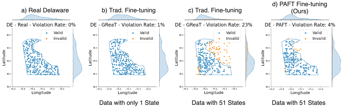
Figure 1: Synthetic location data generated by GReaT for the state of Delaware (DE) in the United States, where the solid line represents the official border of Delaware and the blue and yellow colors indicate the legal and illegal samples in the synthetic data respectively. Traditional GReaT fine-tuning with random order permutation (Fig 1 b) works well for one state at a time but creates datasets with egregious violations when applied to all 51 states (Fig 1 c). PAFT, our fine-tuning approach that utilizes an established optimal fine-tuning order, significantly mitigates the challenges posed by this complex dataset (Fig 1 d). 51 states includes (50 US states + Washington DC).

In the field of tabular data generation, generative models that focus on conditional distribution learning (auto-regressive models [42] and LLM [3]) have a distinct advantage over generative models based on joint distribution learning (GAN [40], VAE [40, 43], and Diffusion [43]). These models excel at accurately generating conditional constraints between columns, both in theory and in practice [11, 3]. However, the performance of existing conditional generation techniques can differ depending on the dataset, and even within different categories of the same dataset. It is worth noting that this paper analyzes conditional constraints between various types of attributes, rather than just focusing on numerical correlations. These conditional constraints often exhibit asymmetry, which has the potential to greatly influence the training and generation process of the model.

2.1 Can LLMs model composite datasets?

By a composite dataset, we mean one that is best modeled as a mixture of distributions rather than a single distribution for the full table. The traditional approach to fine-tuning pioneered by methods such as GReaT work only if we assume that the table can be modeled by a single distribution rather than a mixture. For instance, in a geolocation dataset, fine-tuning with GReaT works for one US state at a time.

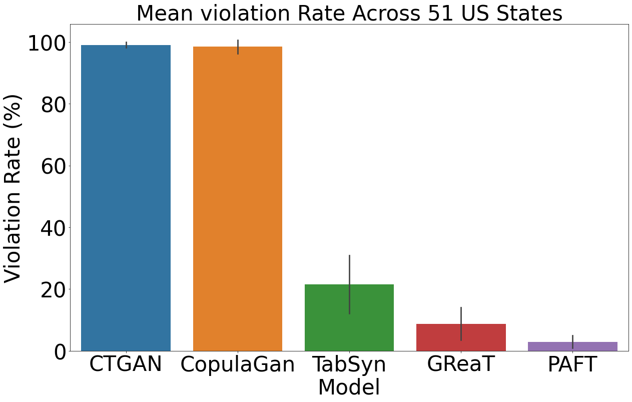
Figure 2: For a composite dataset, comparison of state-specific violation rates for different synthetic data generation approaches. The states (x-axis) are sorted based on increasing violations. PAFT significantly mitigates state-specific violations in a composite dataset.

In Fig. 1, we aim to generate synthetic location data made up of (latitude, longitude) tuples for US states. Fig. 1 (a) depicts sampled real locations for the state of Delaware (DE) chosen for its irregular shape. In Fig. 1 (b), we depict the results from GReaT which shows a very admirable 1% violation rate. Following their approach, we fine-tune the Distill-GPT2 LLM [35] by supplying tuples of (latitude, longitude, state) in a randomized order.

However, when we extend this method to all 51 US states and territories, we can see that the generated data for Delaware drops significantly in quality, with violations growing to 23% after fine-tuning (Fig. 1 (c)). Generated data for other states suffer from similar violations. With our fine-tuning approach (PAFT) presented later (Fig. 1 (d) we are able to support the generation of synthetic data for all 51 states with minimal violations.

Observation 1: Modeling one class can be done in an order-agnostic manner but modeling a multi-class dataset requires paying careful attention to feature ordering.

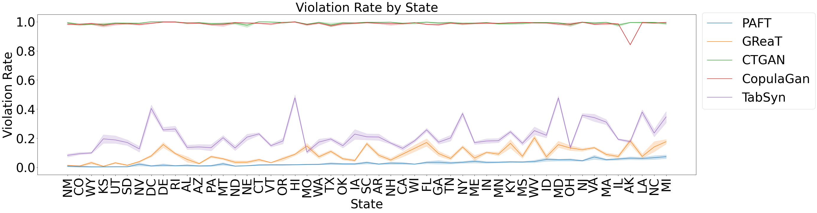
Figure 10: For a composite dataset, comparison of state-specific violation rates for different synthetic data generation approaches. Here, the states (x-axis) are sorted based on increasing violations. PAFT significantly mitigates state-specific violations in a composite dataset.

Observation 2:. Within a composite, multi-class, dataset, there is variance in difficulty of modeling specific classes (e.g., New Mexico is easier to model for LLMs than Delaware or Alaska). See Fig. 5 and Fig. 10 in Appendix.

2.2 How does the importance of feature order vary with schema complexity?

Observation 3: While any order can achieve satisfactory results for unmixed data, it becomes increasingly crucial to employ a better order when the dataset becomes progressively more composite. We conduct a simple experiment based on a simulated table with four attributes and corresponding six column-wise dependencies (see Appendix C.1). Figure 3 shows the relationship between different order permutations. In this simulated table, there are a total of six dependencies between columns (to be made precise using the notion of FDs later); see Appendix C.1. The evaluation measure captures the extent to which the generated data preserves the functional dependencies present in the original data, so that 6 means the generated data is faithful to the original schema complexity and 0 means the data has maximum violations. From Figure 3, we observe that as the schema complexity increases (progressively adding more classes from left to right), it becomes increasingly important to establish a precise sequence in order to provide higher quality generated data. Thus, with randomly guessed order permutations, auto-regressive generation with LLMs are severely limited in their ability when it comes to simulating composite datasets with complex functional dependencies.

2.3 How susceptible are LLMs and other models to sacrificing conditional nuance in favor of capturing joint distributions?

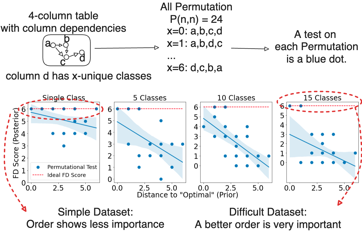
Figure 3: For a simulated table with a total of 6 functional dependencies (FDs), we showcase increased FD violations as the dataset becomes progressively more composite (increasing classes). x-axis represents degree of deviation of data permutation from ideal permutation while y-axis represents number of retained FDs (higher is better, with FD = 6 being optimal). Each blue dot in a graph represents a single possible permutation of the data in fine-tuning process. Thus, while order permutation may not be as crucial for unmixed datasets (left), permutation order becomes important as dataset complexity increases (right).

A recently presented paper, TabSyn [43], showcased remarkable advancements in joint-distribution learning generative models, surpassing previous models of similar lineage, in terms of distributional correlation measures and machine learning efficiency. However, as we will show, methods like TabSyn fail to capture real-world dependencies, e.g., the relationship between protocol and port number in network traffic data [42], or the geographical boundaries of US states as described earlier. Constraints in tabular data can be inferred empirically from conditional distributions in the data and thus methods such as LLMs are particularly powerful because of their autoregressive nature.

Observation 4: While joint distribution learning models (CTGAN [40], CorpulaGAN [40], TabSyn [43]) and conditional distribution models (GReaT and ours) exhibit comparable performance in modeling joint distributions, LLM-based fine-tuning demonstrates greater advantages for capturing conditional distributions, functional relationships, and domain constraints (see Figure 5 and Table 2).

In summary, feature ordering can be both a nuisance and a gift. It is a nuisance because it demands additional constraints to be modeled. It can be a gift because it suggests ways to sequentially generate data even by autoregressive LLMs. Our proposed approach (PAFT ) aims to achieve an optimal permutation order for fine-tuning LLMs.

3 PAFT : Permutation-Aided Fine-Tuning

Problem Setup. Let $\mathcal{D}$ represent a table with $n$ rows (i.e., records) and $m$ columns (i.e., attributes a.k.a schema). Let each record be represented by vector $\mathbf{x}_{i}$ and further let $x_{ij}$ represent the element value of the $j^{th}$ attribute of record $\mathbf{x}_{i}$. Hence each row $\mathbf{x}_{i}\in\mathcal{D}$ represents an individual record and each column $\mathbf{x}_{(:,j)}\sim\mathcal{X}_{j}$ can be considered sampled from a random variable $\mathcal{X}_{j}$ that governs the distribution of attribute $j$. Finally, let $i\in[1..n]$ and $j\in[1..m]$. Realistically, tabular data $\mathcal{D}$ is frequently a mixture of categorical and continuous attributes, hence each $\mathcal{X}_{j}$ can be a categorical or continuous random variable. If $\mathcal{A}=\{\mathcal{X}_{1},\mathcal{X}_{2},\dots,\mathcal{X}_{m}\}$ represents the collection of random variables, then the table generation process aims to sample from a joint distribution $\mathbb{P}(\mathcal{A})=\mathbb{P}(\mathcal{X}_{1},\mathcal{X}_{2},\dots,\mathcal{X}_{m})$. This joint distribution is usually a complex, high-dimensional distribution and, most importantly, unknown. The goal of learning an effective tabular data generator $p_{\theta}(\cdot)$ is to enable $p_{\theta}(\cdot)$ to learn a faithful approximation $\mathbb{P}(\mathcal{A}|\mathcal{D})$ of the data generation process distribution $\mathbb{P}(\mathcal{A})$ using the data sample $\mathcal{D}$ such that $\mathbb{P}(\mathcal{A}|\mathcal{D})\approx\mathbb{P}(\mathcal{A})$. Once such an effective model $p_{\theta}(\mathcal{D})$ is trained, it can be employed to generate large volumes of seemingly realistic synthetic data $\mathcal{\hat{D}}\sim\mathbb{P}(\mathcal{A}|\mathcal{D})$.

3.1 Tabular Data Generation with LLMs

While training $p_{\theta}(\cdot)$, it is usually assumed that all records $\mathbf{x}_{i}\in\mathcal{D}$ are independent. Generating new data samples $\hat{\mathbf{x}}_{i}\in\hat{\mathcal{D}}$ can be done in various ways (e.g., see [41, 40, 45]) which aim to directly estimate the joint distribution $\mathbb{P}(\mathcal{A})$ or, as is done here in PAFT , where $\mathbb{P}(\mathcal{A})$ is estimated by an autoregressive LLM based generative process, as a product of multiple conditional densities governed by the input ordering.

Autoregressive LLM models are pre-trained to maximize the likelihood of target token $x_{ij}\in\mathcal{D}$, conditioned upon the autoregressive context $\mathbf{x}_{(i,1:j-1)}\in\mathcal{D}$ where $\mathcal{D}$ is the training corpus comprising a large amount of textual data (in the pre-training context). Eq. 1 defines the general training criterion of LLM training using the self-supervised next-token prediction task with ‘w’ denoting the context length.

$$\mathcal{L}(\theta;\mathcal{D})=-\sum\limits_{\mathbf{x}_{i}\in\mathcal{D}}\sum\limits_{j=1}^{w}\mathrm{log}\,\mathbb{P}(x_{i}|\mathbf{x}_{(i,1:j-1)})$$ (1)

The generation of a single instance (i.e., database record) $\mathbf{x}_{i}\in\mathcal{D}$ is given by Eq. 2:

$$\mathbb{P}(\textbf{x}_{i})=\mathbb{P}(x_{i,1},...,x_{i,m})\simeq\prod_{j=1}^{m}\mathbb{P}(x_{i,j}|x_{i,1},..,x_{i,j-1})$$ (2)

Specifically, each database record is generated as a product of conditional distributions.

Input Encoding. To support the processing of our records $\mathbf{x}_{i}\in\mathcal{D}$ by a pre-trained LLM, we adopt the following encoding:

$$\begin{split}t_{i,j}=[c_{j},\textrm{`}is\textrm{'},x_{i,j},\textrm{`},\textrm{'}],&i\in\{1,..,n\},j\in\{1,..,m\},\\ \mathbf{t}_{i}=[t_{i,1},t_{i,2},..,t_{i,m}],&i\in\{1,..,n\}\end{split}$$ (3)

In Eq. 3, $c_{j}$ represents the attribute name of the $j^{th}$ database column while $x_{i,j}$ represents the actual value of the $j^{th}$ column for the $i^{th}$ record. Further, we can assume we have a mechanism to obtain a feature order permutation $\mathbf{k}$ to govern the order of the attributes in $\mathbf{t}_{i}$, such that $\mathbf{t}_{i}(\mathbf{k})=[t_{i,k_{1}},t_{i,k_{2}},..,t_{i,k_{m}}]$ (where $i\in\{1,..,n\},k_{j}\in\{1,..,m\}$.), represents the same record but with the attribute order governed by the permutation $\mathbf{k}$, This definition admits the random feature order as a special case in which $\mathbf{k}$ is a random permutation.

Since we consider autoregressive LLM-based generative models, employing the chain rule to sequentially produce each column of a table record $\mathbf{t}_{i}$, we can view each generation step as approximating the joint distribution of the table columns as a product of conditional distributions (i.e., $\mathbb{P}(t_{i,1},...,t_{i,m})\simeq\prod_{j=1}^{m}\mathbb{P}(t_{i,j}|t_{i,1},..,t_{i,{j-1}})$). However, as the number of columns increases and the relationships between columns get more conditional, the likelihood of encountering training and sampling bias due to class imbalance also rises [40]. To minimize such adverse effects, we can consider injecting knowledge of the pre-existing functional relationships among columns, to govern the autoregressive generation process. To infer such functional relationships, we leverage a learned dependency graph derived from functional dependency (FD) relations which enables us to effectively determine the appropriate training and sampling sequence. This, in turn, allows us to alleviate potential biases during training by establishing a generation curriculum leading to improved estimation accuracy of the joint distribution $\mathbb{P}(\textbf{t}_{i})$ in auto-regressive prediction $\mathbb{P}(t_{i,k_{1}},...,t_{i,{k_{m}}})\simeq\prod_{j=1}^{m}\mathbb{P}(t_{i,k_{j}}|t_{i,k_{1}},..,t_{i,k_{j-1}})$, where the ordering $t_{i,k_{1}}\dots,t_{i,k_{m}}$ is obtained by a feature order permutation function $\mathbf{k}=\phi(\mathcal{D},\mathcal{S})$. We detail the requisite background and design of $\phi(\mathcal{D},\mathcal{S})$ in sections 3.2 and  3.3.

3.2 Discovery and Distillation of Functional Dependencies (FD)

A functional dependency (FD) is a relationship $R$ in schema $S$ that exists when a subset of attributes $A\subset S$ uniquely determines another subset $B\subset S$ of attributes. We succinctly represent an FD as $R:A\rightarrow B$ which specifies that $B$ is functionally dependent on $A$. FDs can be record-level or schema-level.

Definition 1 (Record-Level FD).

With $A$, $B$ being two disjoint subsets of the schema (columns) of table $\mathcal{D}$, let $a\in A$, $b\in B$ denote two entries in A and B; a record-level FD f has the form: $f:a\rightarrow b$.

Definition 2 (Schema-Level FD).

With $A$, $B$ being two disjoint subsets of the schema (columns) of table $\mathcal{D}$, a schema-level FD $F$ associated with $\mathcal{D}$ has the form: $F:A\rightarrow B$.

We leverage FD discovery techniques to govern the order of the autoregressive data generation process in PAFT . A large body of research from the database literature on FD discovery [26, 44, 27] can be leveraged in PAFT , including methods that account for noisy FDs [44]. In this work, we focus on leveraging schema-level FDs discovered using a state-of-the-art FD discovery algorithm [27] to govern the autoregressive data generation process.

FD Distillation. The result of traditional FD discovery, yields complex (i.e., multi-attribute) functional dependencies between columns which are ambiguous to resolve in an autoregressive generation setting. Hence we undertake an intermediate FD distillation step to simplify multi-attribute functional dependencies into multiple single attribute FDs as detailed below.

We first construct a dependency graph model $G(\mathcal{V},\mathcal{E})$ where $\mathcal{V}$ represents the set of vertices with each $v\in\mathcal{V}$ representing an attribute in $\mathcal{S}$ and $e_{ij}\in\mathcal{E}$ representing an edge relation from attribute $v_{i}$ to attribute $v_{j}$. Further, we consider two types of edges in $\mathcal{E}$, specifically each $e_{ij}$ may be a type-1 edge or a type-2 edge (defined next). The two edge types (i.e., type-1, type-2) in $\mathcal{E}$ are derived from three classes of FDs, as shown in Fig. 4(a). Subsequently, we proceed to examine each individual case: 1) Single attribute left-hand side (LHS) and single attribute right-hand side (RHS) 2) Multi-attribute LHS and single-attribute RHS. 3) single or multi-attribute LHS and multi-attribute RHS. We shall use the example table in Fig.  6 to define each FD case.

[Type-1 Edge]. Let us consider an example of FD Case 1, wherein the column State functionally determines column Bird. In such a case, we enforce that the value for the attribute State be generated prior to the value for the attribute Bird. Accordingly, a forward directed edge from State to Bird is created in the column dependency graph $\mathcal{G}$. We term such forward directed edges as type-1 edges in $\mathcal{G}$. [Type-2 Edge]. The other type of edge in $\mathcal{G}$, arises when we encounter an FD with a multi-attribute LHS and a single attribute RHS (i.e., FD Case 2). As per FD Case 2, the values of multiple columns in the LHS would collectively decide the value of the column on the RHS. As an example in Fig. 4(a), the tuple of columns Latitude, Longitude functionally determines State. For such FDs, two backward edges are added in the column dependency graph $\mathcal{G}$, connecting State to both Latitude and Longitude. We term such backward directed edges as type-2 edges in $\mathcal{G}$.

FD Case 3 relationships are ones where the RHS has multiple attributes and the LHS could have single or multiple-attributes. Such relationships do not directly result in an edge in our dependency graph $\mathcal{G}$. Instead, as classically done in FD literature [27], we subject such FD relationships to an intermediate decomposition step. Specifically, the multi-attribute RHS of FD Case 3 relationships is decomposed into multiple single-attribute RHS dependencies each comprising the original LHS. Further, in each of these new decomposed relationships, if the LHS is single-attribute, it is treated as a FD Case 1 relationship (i.e., a directed edge from $LHS$ to $RHS$ is added to $\mathcal{G}$), else it is handled as an FD Case 2 relationship, wherein for each attribute in the multi-attribute LHS, a backward dependency edge from the single-attribute RHS is added to the dependency graph $\mathcal{G}$. Therefore, for every column in the right-hand side (RHS), we employ either type-1 or type-2 edge construction, depending on the value of its left-hand side (LHS). Full procedure detailed in Appendix A.2 Algorithm 1 .

3.3 Putting It All Together

Until this point, our construction of the graph $\mathcal{G}$ has only been limited to considering pair-wise relationships between columns in $\mathcal{D}$. Graph properties like functional dependency transitivity, require us to obtain a total ordering on the nodes $v\in\mathcal{V}$ of $\mathcal{G}(\mathcal{V},\mathcal{E})$ that is deterministic in nature for effective auto-regressive LLM training. This implies that in order to obtain a feature order permutation ($\mathbf{k}$) from the derived functional dependency relationships (Sec. 3.2), a computation must be performed on the entire dependency graph $G(\mathcal{V},\mathcal{E})$.

We define this task of obtaining a total feature order $\mathbf{k}$ from $\mathcal{G}(\mathcal{V},\mathcal{E})$ as an optimization step which seeks to produce $\mathbf{k}$ while minimizing the number of violated relationships in $\mathcal{G}(\mathcal{V},\mathcal{E})$. Appendix A.2 Algorithm 2 outlines this procedure.

Consider the trivial case of having an empty FD graph $\mathcal{G}$ i.e., $|\mathcal{E}|=\emptyset$. If the columns of a table are not functionally dependent on each other, then the order of generation is not important and $\mathbf{k}$ can be some arbitrary permutation of the columns in $\mathcal{S}$. For all other cases, our total feature ordering algorithm operates in three phases, as shown in Fig. 4(b). [Phase 1: Condensation]. It is apparent that if a graph is not a directed acyclic graph (DAG), there is no optimal solution to the total feature ordering problem. In other words, there must be FDs that cannot be satisfied in the resulting total order permutation $\mathbf{k}$. In such cases, we compute the strongly connected components (SCC), and condense them into super nodes, thus transforming the original graph into a DAG. [Phase 2: Ordering]. An application of a topological sort onto the DAG from Phase 1 will result in a total feature ordering with all SCCs in $\mathcal{G}$ compressed into super nodes. [Phase 3: Expansion of SCC]. Once the topological sort is conducted in Phase 2, we finally expand the SCC super nodes (via. arbitrary ordering) such that although the intra-SCC ordering of the nodes within the SCC is arbitrary, their ordering relative to non-SCC nodes is maintained.

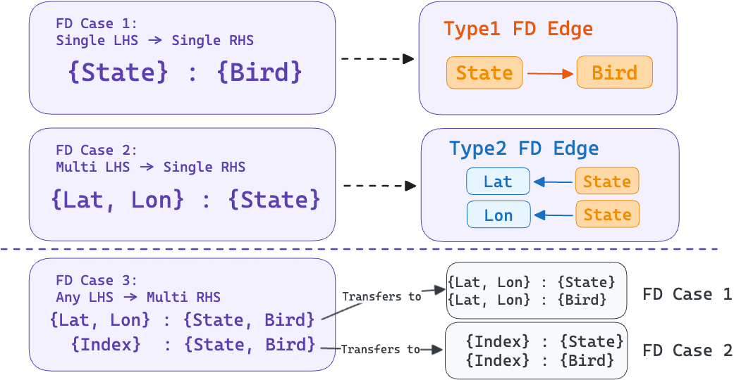
(a) There are two types of column dependency edges for three types of functional dependencies (FDs), which are distinguished by the left-hand side (LHS) and right-hand side (RHS) in the FD.

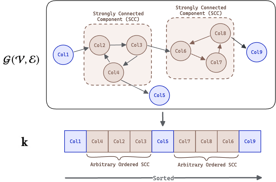
(b) DAG for column functional dependency derived by expanding SCC super nodes and retrieving a fully flattened, ordered structure.

Figure 4: PAFT: FD-Distillation and Depdendency Graph Sorting

3.4 Synthetic Data Generation using PAFT 

After the optimized feature order permutation is obtained (via Appendix A.2 Algorithm 2), we fine-tune the LLM with the textually encoded table record $\mathbf{t}_{i}$ such that the auto-regressive generation process is governed by the optimal feature order permutation $\mathbf{k}=\phi(\mathcal{D},S)$. Specifically, we generate the table governed by order $\mathbf{k}$ as defined in Eq. 4.

$$\mathbb{P}(\textbf{t}_{i})=\mathbb{P}(t_{i,k_{1}},...,t_{i,{k_{j}}})\simeq\prod_{j=1}^{m}\mathbb{P}(t_{i,k_{j}}|t_{i,k_{1}},..,t_{i,k_{j-1}})$$ (4)

We employ the Low-Rank Adaptation (LoRA) fine-tuning strategy [16]. To generate synthetic rows, we first sample the initial token $p(t_{i,k_{1}})$ from the marginal distribution of variable $k_{1}$ in actual training data, and then use Eq. 4 to sequentially sample subsequent tokens $p(t_{i,k_{j}})$, where $j\in{2,...,m}$.

4 Experimental Evaluation

In this section, we empirically evaluate PAFT using multiple qualitative and quantitative measures. Specifically, we investigate 7 research questions (see Table 1) to inspect the generation prowess of PAFT with respect to state-of-the-art models while also investigating the degree to which PAFT generated synthetic data is faithful to real-world data distributions and functional dependencies.

ID	Research Question	Section
RQ1	How do complex data characteristics affect generation quality?	Sec. 4.2
RQ2	Does PAFT generate data consistent with intrinsic data characteristics?	Sec. 4.3
RQ3	Can data generated by PAFT replace real data in downstream ML model training?	Sec. 4.4
RQ4	Does PAFT adhere to real distributions and exhibit mode diversity?	Sec. B.1
RQ5	Does the synthetic data generated by PAFT pass the sniff test?	Sec. B.2
RQ6	Can PAFT enhance the stability in generating high quality tables, resulting in a faster sampling phase?	Sec. B.3

Table 1: Research questions investigated in our work.

4.1 Dataset and Baseline

Dataset. We evaluated the efficiency of PAFT through experiments on six real datasets commonly used in synthetic table generation studies like GReaT [3] CTGAN [40]. These are: Beijing [7], US-locations [13], California Housing [24], Adult Income [2], Seattle [34], and Travel [37]. Separately we also generate a set of four simulated datasets (as described in Algorithm 3 Appendix C.1). Details of dataset statistics are in the Appendix C.1.

Baseline. In benchmarking suite, we have baselines that consist of current deep learning approaches for synthetic data generation (CTGAN [40], CopulaGAN [40], TabSyn [43]), and the most advanced LLM fine-tuning synthetic table generator GReaT [3]. To guarantee an equitable comparison, we employ the Distill-GReaT model for both LLM techniques in all tests. Details in Appendix C.2.

4.2 RQ1: How do complex data characteristics affect generation quality?

Figure 1 has shown that generating a mixture-class of data is more challenging than generating single-class data for baseline methods. However, our approach is capable of effectively handling this task. In order to emphasize the conditional distribution between two columns, we will also assess the performance of our technique and the baseline method for various classes within a mixture-class dataset.

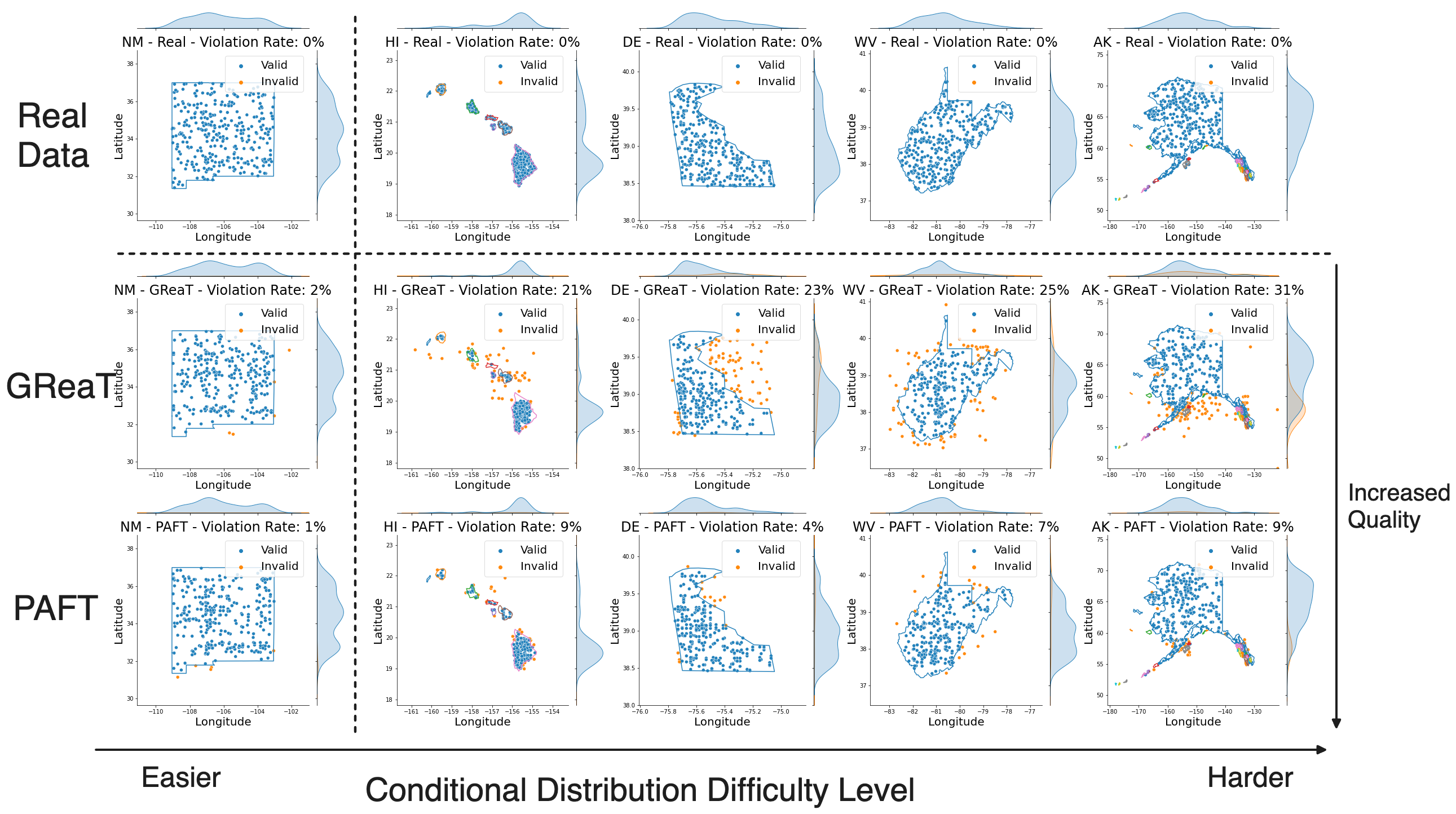
Figure 5: Different states depict different complexity levels for an LLM to fine-tune with. The semantic complexity level increases from left to right. We demonstrate that, in comparison to baselines, PAFT effectively decreases instances of violations (represented by the color orange) in the generated data. Violation rate refers to occurrence of instances that transgress boundaries of a state.

Figure 5 and 10 illustrates that various classes within a complicated dataset may present distinct challenges when it comes to modeling, respectively in terms of visualization and statistics. Both baseline and PAFT can provide satisfactory performance in less complex classes. As the level of complexity rises, the importance of finding the most optimal permutation becomes crucial, and hence we find that PAFT , which is aware of the functional dependencies and hence able to better capture semantic structure in the data, outperforms the GReaT baseline which is agnostic of functional dependencies. The variation may arise due to statistical factors or semantic factors in the actual world, which are examined in a detailed case study (Appendix B.4).

4.3 RQ2: Does PAFT generate data respecting the consistency of intrinsic data characteristics?

We may infer the degree of dependency retention of data’s intrinsic characteristics as another lens through which to evaluate the quality of the data generated by PAFT and baselines. In line with this, we conducted rule checks that were derived from real-world scenarios, and subsequently evaluated the generated data from all DL and LLM baselines, and our PAFT model. Table 2 displays the rate of violation in the generated data. From the table, we observe that PAFT adheres to data’s characteristics more faithfully (i.e., significantly fewer rule violations) than baseline methods, by learning together with functional dependencies.

Dataset	Intrinsic Fact	CTGAN	CopulaGAN	TabSyn	GReaT	PAFT
US-locations	State_code $\rightarrow$ bird	94.66$\pm$0.32%	95.66$\pm$0.17%	0.10$\pm$0.04%	0.30$\pm$0.00%	0.00$\pm$0.00%
US-locations	Lat-long $\rightarrow$ State	99.22$\pm$0.08%	98.51$\pm$0.07%	21.50$\pm$0.32%	8.16$\pm$0.14%	2.93$\pm$0.15%
California	Lat-long $\rightarrow$ CA	47.56$\pm$6.37%	99.93$\pm$0.00%	8.83$\pm$0.13%	5.42$\pm$0.16%	1.26$\pm$0.06%
California	Median house price $\rightarrow$ [1.4$e^{5}$, 5$e^{5}$]	1.46$\pm$1.52%	0.01$\pm$0.01%	0.00$\pm$0.00%	0.00$\pm$0.00%	0.00$\pm$0.00%
Adult	education $\rightarrow$ education-num	83.94$\pm$ 1.93%	19.09$\pm$ 0.58%	1.43$\pm$0.04%	1.24$\pm$0.09%	0.46$\pm$ 0.03%
Seattle	Zipcode $\rightarrow$ Seattle	0.00$\pm$0.00%	99.88$\pm$0.00%	0.00$\pm$0.00%	0.00$\pm$0.00%	0.00$\pm$0.00%

Table 2: Datasets exhibit a range of intrinsic characteristics: functional dependencies, range restrictions, and other types of domain knowledge. Cells denote percentage of violations in generated data.

Method		Orig.	CTGAN	CopulaGAN	TabSyn	GReaT	PAFT
Beijing (*) ($\downarrow$)	RF	0.41%	2.49$\pm$0.57%	2.15$\pm$0.29%	0.7$\pm$0.01%	0.57$\pm$0.00%	0.52$\pm$0.00%
	LR	1.37%	2.23$\pm$0.54%	1.55$\pm$0.21%	1.25$\pm$0.0%	0.97$\pm$0.01%	1.34$\pm$0.01%
	NN	0.99%	2.44$\pm$0.74%	2.83$\pm$1.18%	1.01$\pm$0.14%	1.16$\pm$0.56%	0.95$\pm$0.13%
California (*) ($\downarrow$)	RF	0.18%	0.65$\pm$0.09%	0.39$\pm$0.01%	0.22$\pm$0.0%	0.25$\pm$0.00%	0.20$\pm$0.00%
	LR	0.30%	0.54$\pm$0.1%	0.5$\pm$0.01%	0.30$\pm$0.0%	0.29$\pm$0.00%	0.31$\pm$0.00%
	NN	0.34%	0.53$\pm$0.11%	0.47$\pm$0.02%	0.29$\pm$0.02%	0.3$\pm$0.01%	0.27$\pm$0.00%
Seattle (*) ($\downarrow$)	RF	0.33%	0.76$\pm$0.34%	0.38$\pm$0.07%	0.30$\pm$0.06%	0.35$\pm$0.01%	0.28$\pm$0.03%
	LR	0.29%	0.74$\pm$0.35%	0.32$\pm$0.03%	0.23$\pm$0.04%	0.33$\pm$0.00%	0.29$\pm$0.03%
	NN	0.28%	0.71$\pm$0.33%	0.38$\pm$0.08%	0.28$\pm$0.01%	0.33$\pm$0.00%	0.27$\pm$0.01%
US-locations ($\uparrow$)	RF	99.95%	7.17$\pm$1.58%	45.33$\pm$2.82%	99.99$\pm$0.01%	99.84$\pm$0.07%	99.91$\pm$0.03%
	LR	46.1%	5.11$\pm$3.14%	31.08$\pm$1.92%	43.69$\pm$1.9%	45.65$\pm$0.86%	49.41$\pm$1.57%
	NN	99.85%	7.56$\pm$4.61%	53.34$\pm$1.59%	99.64$\pm$0.17%	98.94$\pm$1.16%	99.44$\pm$0.28%
Adult ($\uparrow$)	RF	84.97%	71.15$\pm$5.59%	81.33$\pm$1.53%	83.69$\pm$0.28%	83.89$\pm$0.42%	83.06$\pm$0.35%
	LR	78.53%	75.68$\pm$0.14%	78.18$\pm$ 1.53%	78.38$\pm$0.11%	76.1$\pm$0.29%	77.24$\pm$0.09%
	NN	76.9%	75.69$\pm$0.10%	76.6$\pm$1.26%	78.36$\pm$1.23%	78.23$\pm$1.31%	79.16$\pm$0.15%
Travel ($\uparrow$)	RF	88.95%	56.35$\pm$2.64%	67.18$\pm$3.0%	84.09$\pm$1.18%	79.78$\pm$1.29%	85.19$\pm$1.99%
	LR	82.87%	70.17$\pm$17.46%	79.56$\pm$0.00%	83.31$\pm$0.22%	78.34$\pm$2.02%	82.76$\pm$1.01%
	NN	81.77%	71.05$\pm$17.85%	79.56$\pm$0.00%	81.88$\pm$1.33%	80.77$\pm$1.33%	83.2$\pm$0.9%

Table 3: MLE Performance (%): Comparison of original data to synthetic data. For datasets denoted as (*), we use a regression model for prediction, and calculate MAPE as performance (where lower scores are ideal); For other datasets, classification models are used for prediction and we calculate the accuracy as performance. The best results are marked in bold and the second-best results are underlined. RF: random forests; LR: linear regression: NN: a traditional multi-layer perceptron.

4.4 RQ3: Can data generated by PAFT replace real data in downstream ML model training?

We next assesses effectiveness of the generated (i.e., synthetic) data by measuring how well discriminative models trained on synthetic data perform on their target discrimination task versus when trained on real data. As shown in Table 3, PAFT  is best or second best in over 80% of (dataset, method) combinations. Other research questions are discussed in the appendix, as indicated in Table 3.

5 Conclusion

This work has brought LLMs closer to the goal of generating realistic synthetic datasets. By learning FDs and leveraging this information in the fine-tuning process, we are able to align the auto-regressive nature of LLMs with the ordering of columns necessary for generating quality synthetic data. While PAFT is quite broadly applicable by itself, it can be extended in several directions. First, what are other, perhaps more expressive, types of tabular constraints that can be utilized in the fine-tuning process? Second, what is the internal basis for regulating orders inside a transformer architecture and can we more directly harness it? Third, can we theoretically prove the (im)possibility of generating specific synthetic datasets by LLM architectures? Fourth, despite the numerous advantages of LLM in learning and generating tabular data, scalability remains an acknowledged challenge [11, 3, 14], encompassing concerns such as context window and training speed. And finally, privacy-preserving methods have been implemented in table generators based on GANs but remains understudied in LLM fine-tuning. These questions will be the focus of our future work.

Limitations. The row-wise generation cost of our method, particularly when employing fine-tuning, is affected by the dataset sample size and computational resources (GPU). Moreover, the capacity of PAFT to generate columns is affected by context window sizes. These limitations can be overcome by the newer generation of LLMs or by exploring partial row generation, i.e., generating a row in multiple steps using an LLM.

Appendix A Extended Methodology

A.1 Method Overview

Figure 6 shows an overview of the proposed permutation aided fine-tuning approach (PAFT ). A typical workflow is 1) Textual Encoding (Section 3.1) 2) Functional Dependency (FD) discovery (Section 3.2) 3) FD Distillation ( Section 3.2)and 4) The Feature Order Permutation Optimization ( Section 3.3). Fine-tuning and sampling Strategy is explained in Section 3.4.

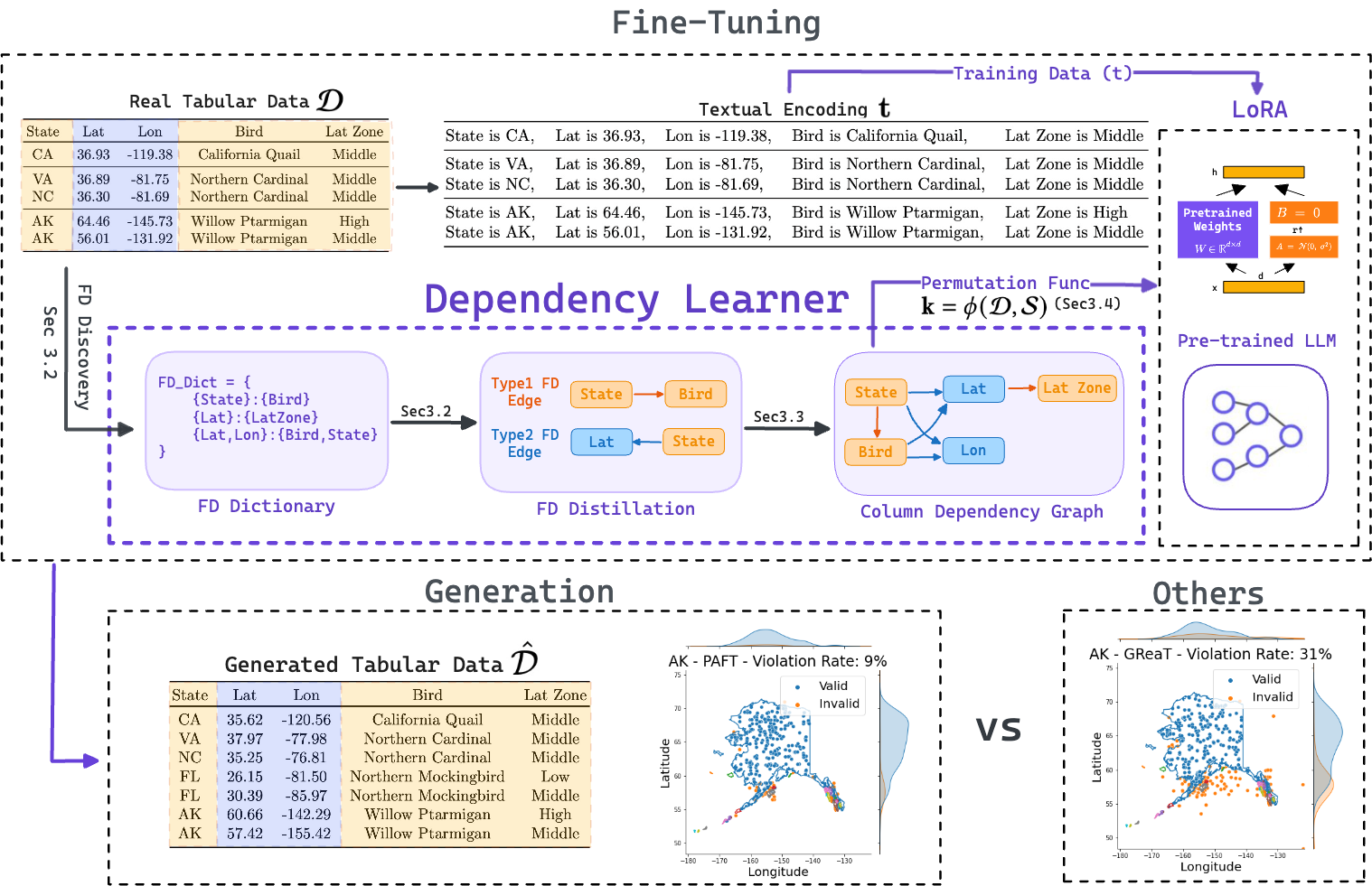
Figure 6: Overview of the proposed Permutation-Aided Fine-tuning (PAFT ) approach.

A.2 Extended Algorithm

Algorithm 1 details FD distillation procedures corresponding to the text in Section 3.2 and Algorithm 2 details Feature Order Permutation Optimization procedures corresponding to the text in Section 3.3.

Algorithm 1 FD Distillation with Schema-Level FDs

1:List of Schema-level FDs, $\mathcal{S}$

2:Column Dependency Graph, $\mathcal{G}(\mathcal{V},\mathcal{E})$

3:$\mathcal{G}\leftarrow\emptyset$

4:for $fd\in\mathcal{S}$ do

5:     $LHS,RHS\leftarrow fd$

6:     if $LHS.length=1$ and $RHS.length=1$ then

7:         for $u\in LHS$ do

8:              for $v\in RHS$ do

9:                  $\mathcal{G}.\text{add\_edge}(u,v)$ $\triangleright$ Case 1                        

10:     else if $LHS.length>1$ and $RHS.length=1$ then

11:         for $u\in LHS$ do

12:              $\mathcal{G}.\text{add\_edge}(v,u)$ $\triangleright$ Case 2          

13:     else$\triangleright$ $RHS.length>1$, Case 3

14:         for $v\in RHS$ do

15:              if $LHS.length=1$ then

16:                  $\mathcal{G}.\text{add\_edge}(u,v)$ $\triangleright$ Go to Case 1

17:              else

18:                  for $u\in LHS$ do

19:                       $\mathcal{G}.\text{add\_edge}(v,u)$ $\triangleright$ Go to Case 2                                               

Algorithm 2 Feature Order Permutation Optimization

1:Column Dependency Graphs $\mathcal{G}(\mathcal{V},\mathcal{E})$

2:Optimal Feature Order Permutation $\mathbf{k}$

3:if $|\mathcal{E}|$ = $\emptyset$ then

4:     Return $\mathbf{k}\leftarrow arbitrary\_permutation(\mathcal{V})$

5:if $\mathcal{G}$ is not a Directed Acyclic Graph (DAG) then $\triangleright$ Phase 1

6:     $\mathcal{G}\leftarrow strongly\_connected\_components(\mathcal{G})$

7:$\mathbf{k}\leftarrow topological\_ordering(\mathcal{G})$ $\triangleright$ Phase 2

8:$\mathbf{k}\leftarrow arbitrary\_SCC\_expansion(\mathcal{G})$ $\triangleright$ Phase 3

9:Return $\mathbf{k}$

Appendix B Additional Research Questions and Case Studies

B.1 RQ4: Does PAFT adhere to real distribution and possess mode diversity?

In this question, we evaluate how closely the density and diversity of the true data distribution are matched by PAFT generated data using correlation metrics and density-based distance metrics. Specifically, we employ Kolmogorov-Smirnov Test (KST) to evaluate the density estimate of numerical columns, and the Total Variation Distance (TVD) for categorical columns. The results for density estimate similarity are detailed in Table 4.

When calculating the correlation between columns, we employ Pearson correlation for numerical columns and contingency similarity for categorical columns. The results for correlation based analysis are detailed in Table 5. The above metrics can be calculated and normalized into the interval of 0-1 with the use of the sdv metric library [10], with 1 indicating that synthetic data perfectly matches real data distribution. Hence, evaluation score allows for easy comparison of data columns, even when they have different types and metrics.

Tables 4 and 5 demonstrate that the PAFT synthetic data closely matches the real data in terms of univariate distribution and bivariate correlation, outperforming the baseline. Visual examples are depicted in Figure 7. PAFT has the ability to generate a wide range of diversity, encompassing both continuous and discrete variables, which closely resembles real data.

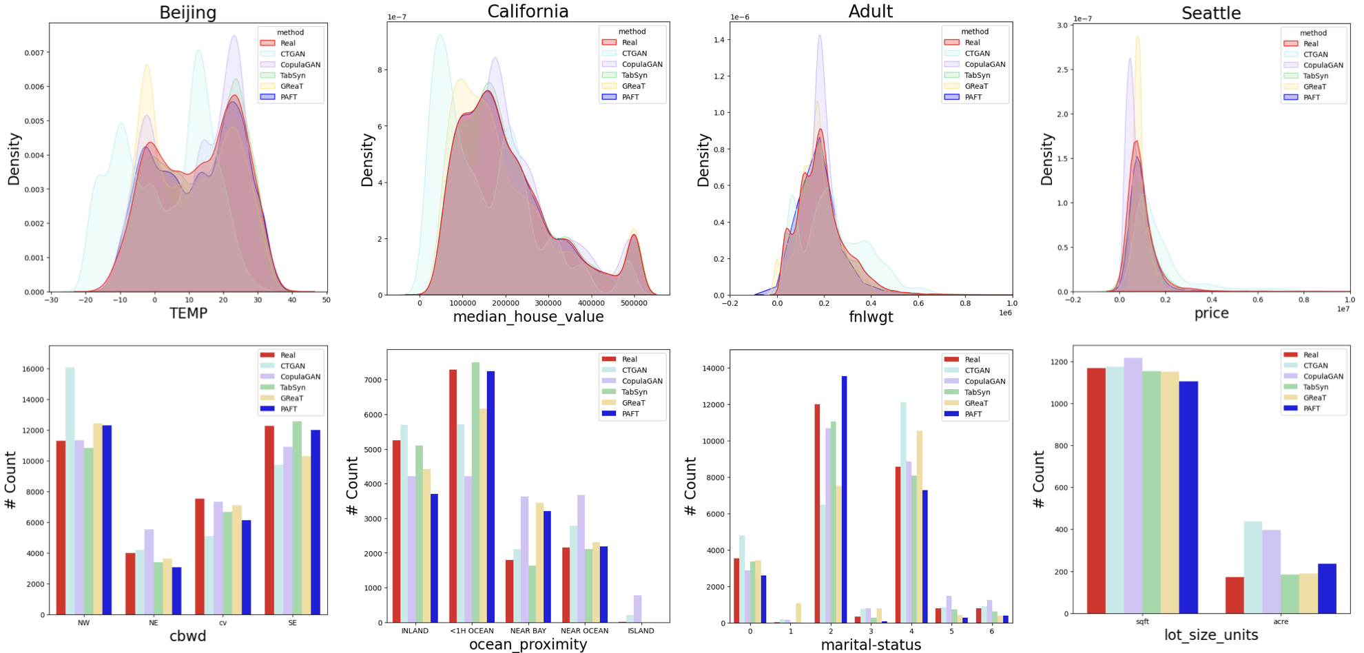
Figure 7: Column distributions for each dataset generated by CTGAN, CopulaGAN, GReaT, and PAFT . Overall, PAFT has the closest distribution to real data compared to other synthesis methods. PAFT also showcase the ability to generate a wide range of diversity.

Dataset	CTGAN	CopulaGAN	TabSyn	GReaT	PAFT
Adult	0.81$\pm$0.01	0.92$\pm$0.01	0.98$\pm$0.00	0.88$\pm$0.00	0.90$\pm$0.00
Beijing	0.89$\pm$0.01	0.79$\pm$0.01	0.98$\pm$0.00	0.93$\pm$0.00	0.97$\pm$0.00
California	0.87$\pm$0.03	0.77$\pm$0.01	0.98$\pm$0.00	0.89$\pm$0.00	0.83$\pm$0.00
US-locations	0.83$\pm$0.02	0.82$\pm$0.00	0.96$\pm$0.00	0.93$\pm$0.00	0.97$\pm$0.00
Seattle	0.83$\pm$0.01	0.73$\pm$0.02	0.93$\pm$0.00	0.90$\pm$0.00	0.93$\pm$0.00
Travel	0.84$\pm$0.01	0.90$\pm$0.02	0.93$\pm$0.01	0.93$\pm$0.01	0.93$\pm$0.01

Table 4: Error rate (%) of column-wise density estimation [10]. Bold Face represents the best score on each dataset. Higher values indicate more accurate estimation (superior results). PAFT outperforms the best generative baseline model in most case. The best results are marked in bold, the second-best results are underlined.

Dataset	CTGAN	CopulaGAN	TabSyn	GReaT	PAFT
Adult	0.81$\pm$0.02	0.86$\pm$0.01	0.93$\pm$0.00	0.80$\pm$0.01	0.78$\pm$0.00
Beijing	0.92$\pm$0.01	0.94$\pm$0.01	0.99$\pm$0.00	0.95$\pm$0.00	0.98$\pm$0.01
California	0.84$\pm$0.00	0.87$\pm$0.01	0.97$\pm$0.00	0.87$\pm$0.01	0.91$\pm$0.02
US-locations	0.50$\pm$0.02	0.55$\pm$0.00	0.93$\pm$0.00	0.89$\pm$0.00	0.94$\pm$0.00
Seattle	0.74$\pm$0.02	0.72$\pm$0.01	0.80$\pm$0.01	0.76$\pm$0.03	0.81$\pm$0.01
Travel	0.77$\pm$0.02	0.80$\pm$0.02	0.87$\pm$0.01	0.85$\pm$0.01	0.82$\pm$0.05

Table 5: Error rate (%) of pair-wise column correlation score [10]. Bold Face represents the best score on each dataset. PAFT outperforms the best baseline model in most case. The best results are marked in bold, the second-best results are underlined.

B.2 RQ5: Does the synthetic data generated by PAFT pass the sniff test?

Similar to the analysis conducted in recent work [3] (GReaT), we employ the random forest (RF) algorithm to train discriminators to distinguish real data (labelled as True) and synthetically generated data (labeled as False). Subsequently, we test performance on an unseen set (consisting of 50% synthetically generated data and 50% real data). In this experiment, scores represent the percentage of correctly classified entities. In this case, an ideal accuracy score would be close to 50%, which means the discrimniator fails to distinguish between real and synthesized data. Scores are shown in Table 6 and indicate that the data generated by PAFT is most indistinguishable from real data, even by powerful discriminative models.

Method	CTGAN	CopulaGAN	TabSyn	GReaT	PAFT
Beijing	99.16$\pm$ 0.08%	98.69$\pm$ 0.39%	50.97$\pm$0.06%	51.1$\pm$ 0.08%	50.09$\pm$ 0.05%
US-locations	99.94$\pm$ 0.03%	97.74$\pm$ 0.22%	51.97$\pm$0.18%	50.47$\pm$ 0.07%	50.01$\pm$ 0.01%
California	98.35$\pm$ 0.2%	86.64$\pm$ 0.67%	50.64$\pm$0.15%	53.74$\pm$ 0.27%	49.89$\pm$ 0.03%
Adult	94.43$\pm$ 0.53%	59.82$\pm$ 0.9%	51.64$\pm$0.14%	51.12$\pm$ 0.26%	48.75$\pm$ 0.03%
Seattle	87.61$\pm$ 1.06%	85.7$\pm$ 2.0%	50.12$\pm$0.9%	68.27$\pm$ 1.34%	47.21$\pm$ 0.48%
Travel	77.96$\pm$ 1.4%	74.14$\pm$ 1.64%	50.66$\pm$1.97%	62.49$\pm$ 1.2%	48.18$\pm$ 0.81%

Table 6: Discriminator Performance (%): Comparison of synthesized data from CTGAN, CopulaGAN, TabSyn, GReaT, and PAFT . The scores stand for the accuracy for detecting real or fake data, where the ML models are trained using 50% real data and 50% random data. An ideal accuracy score is 50, indicating the model cannot distinguish between real and synthesized data. The best results are marked in bold, the second-best results are underlined.

B.3 RQ6: Can PAFT enhance the stability in generating high quality tables, resulting in a faster sampling phase?

When it comes to the comparison between fine-tuning approaches in LLM, the quality of the generated table rows can be reflected in the sampling process. This is particularly evident when generating an i.i.d row that involves auto-regressive generation. If the generated row cannot be decoded back into a real table row, then another sample needs to be redone. Given that the device condition and hyperparameters of the GReaT and PAFT are identical, a shorter sampling time indicates a higher probability of accepting a generated row, meaning improved generation quality. (See Figure 7.) Furthermore, the time measurement is based solely on a single-core GPU to ensure a fair comparison of different baselines. Using multiple GPU parallel computing can significantly speed up the fine-tuning process in practice.

Admittedly, PAFT and all LLM fine-tuning based table generators share the identical challenge of time consuming (both training and sampling), comparing to classic DL or GAN based table generators. In exchange for the investment of time, there are several advantages to consider. These include the elimination of data preprocessing which is a significant time cost for a human expert in charge of data preparation, a deep understanding of real-world knowledge, and finally DL-bsaed generators have been shown to fail when the table generation task involves generating columns with textual sentences as their values.

	GReaT - Sampling Time	PAFT  - Sampling Time
Adult	37:47 min	5:15 min
Beijing	5:24 min	5:21 min
California Housing	4:16 min	2:58 min
US-locations	58 sec	58 sec
Seattle	10 sec	11 sec
Travel	5 sec	5 sec

Table 7: For certain datasets that pose difficulties for auto-regressive generation (such as Adult), PAFT can significantly enhance the quality of the generation process, resulting in reduced generation time. For typical datasets with fewer challenges, the time-efficiency performance of GreaT and PAFT is comparable. (The standard variance of time in the five random experiments was smaller than one secondary unit, so it has been omitted).

B.4 Case Study: Influence of Statistical and Semantic Factors

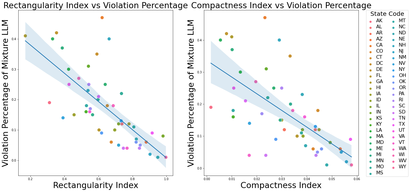
Figure 8: Semantic Complexity: using the random order permutation to modeling the mixture of states data is more challenging when the rectangularity index (left) and compactness index (right) increase.

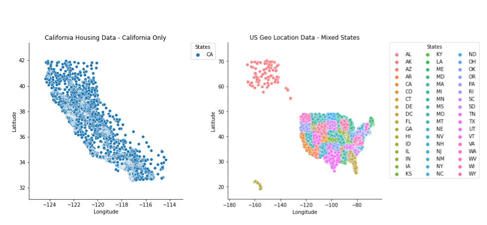
Figure 9: Statistical Complexity can be figured out by analyzing the distribution of the data. For instance, California Housing data is simpler to model concerning the Functional Dependency as it only includes the longitude and latitude for a single state.

Statistical Factor The occurrence of functional dependency in a table is influenced by various factors, including the number of rows and columns, the distinct values in the columns, the relationship between columns, and the presence of duplicate rows, etc. Figure 1 and 8 shows different dataset may have different level of statistic difficulties.

Semantic Factors The acquisition of semantic factors is typically not achievable from direct observation of the data’s appearance. Typically, this implies that the data’s worth will be influenced by real-world expertise in a specific field. For instance, map coordinates are influenced by the geopolitical borders of actual countries and states. Similarly, even if only a subset of data points from a mathematical function are observed, there is a need to comprehend the complete representation of that particular mathematical function.

Fig. 9 shows the difficulty of capturing the functional dependency can also leaded by the semantic conext of a sub-class in a mixture dataset, such as the state shape and geo location distribution. For this case, previous Fig. 5 have already shown the improvement of utilizing PAFT .

Appendix C Data and Experiment Description

C.1 Experimental Setup

Dataset. We evaluated the efficiency of PAFT through experiments on six real datasets commonly used in synthetic table generation studies (GReaT, CTGAN, etc.), as well as a set of four simulated datasets: Beijing [7], US-locations [13], California Housing [24], Adult Income [2], Seattle [34], and Travel [37], Simulated (Algorithm 3). These real-world datasets come from diverse domains and vary in size. The range of the number of functional dependencies spans from 0, indicating complete independence between columns, to around 400, indicating a high level of interdependence. These data also demonstrate the diverse combinations of categories and numerical columns. The simulated data is customized to adhere to the given functional dependence schema, thus explicitly emphasizing the degree to which a model can precisely represent the functional relationship. The simulated data has four distinct versions, denoted by the variable $k$, which represents the unique values in the $d$ column. As the value of $k$ increases, the data becomes more complex, which has been demonstrated to make training the generative model more challenging, as evidenced by all the experimental results presented in this paper. In particular, the functional dependency graph of the simulated data is [$a\rightarrow b$, $a\rightarrow c$,$b\rightarrow c$,$b\rightarrow d$,$a\rightarrow d$,$b\rightarrow d$]. Table 8 provides the FD characteristics of each dataset, while Table 9 provides an more detailed overview.

Training and Testing. To prevent any data leakage, we partitioned the data sets into 80% training sets and 20% test sets. All models are trained or fine-tuned on the same training data samples. All models undergo cross-validation using 5 generated data sets to validate their results. One advantage of using LLM for creating tabular data is that there is no need for any complex data preparation. This means that the feature names and values are used just as they are supplied in the original data sets.

Dataset	Beijing	US-locations	California Housing	Adult Income	Seattle	Travel	Simiulated
# of FDs	157	7	362	78	10	0	6

Table 8: The number of functional dependencies identified using automated FD discovery (Sec 3.2).

Dataset	#Rows	#Cat	#Num	#FD
Beijing	43,824	1	12	157
US-locations	20,400	3	2	7
California	20,640	8	0	362
Adult	32,561	9	6	78
Seattle	2,016	2	6	10
Travel	954	4	3	0
Simulated,k=[1,5,10,15]	10,000	4	0	6

Table 9: Dataset Descriptors (number of rows, categorical columns, numerical columns, and FDs).

Algorithm 3 Building simulated data: Given a dependency graph G, setting values for a table with $n$ rows and $m$ columns with different statistic complexity based on the initial unique value $k$ for the complexity in the root column of the functional dependency chain.

1:procedure SetValues($n,m,G,k$)

2:     $table[n][m]\leftarrow\{\}$

3:     $top\_order,node\_layer\leftarrow Algorithm~{}\ref{alg:optimal_permutation}(G)$

4:     $unique\_value\leftarrow\{\}$

5:     for $vertex\in topo\_order$ do

6:         $top\_value[vertex]=2^{max\_layer-node\_layer[vertex]}$      

7:     for $j\leftarrow 1$ to $m$ do

8:         for $i\leftarrow 1$ to $n$ do

9:              $table[i][j]\leftarrow x_{i\%(top\_value[j]*k)}$               

Baselines. In benchmarking suite, we have baselines that consist of current deep learning approaches for synthetic data generation (CTGAN [40], CopulaGAN [40]), and the most advanced LLM fine-tuning synthetic table generator GReaT [3]. To guarantee an equitable comparison, we employ the Distill-GReaT model for both techniques in all tests, and adjust the hyperparameters as advised by the official GitHub website of GReaT. It ought to mention that GReaT utilizes textual encodings with random feature order permutations. This implies that each sample will undergo a different random order during the training and sampling process. This strategy appears similar to the edge case in Algorithm 2, but in fact, they are distinct. When the FD set is empty, PAFT will suggest a random permutation. Nevertheless, this permutation serves as a comprehensive guide for all samples after an in-depth assessment of FD.

C.2 Reproducibility detail

Baselines. Each baseline (CTGAN, CopulaGAN, TabSyn, GReaT) sticks to the recommended hyperparameters and utilizes officially released API tools: Synthetic Data Vault [28] and GReaT [3]. As for the fair comparison of GReaT and PAFT, the LoRA fine-tuning parameters are set as: Lora attention dimension $r=16$, alpha parameter for Lora scaling $lora\_alpha=32$, The names of the modules to apply the adapter to $target\_modules=c\_attn$, The dropout probability for Lora layers $lora\_dropout=0.05$, $bias=none$.

Computational Resources. To ensure fairness in the comparison between the baselines, all baseline models and experiments were executed on a single Tesla P100-PCIE-16GB GPU.

Parameters for MLE and Discriminator Models. We utilize neural network, linear/logistic regression, and random forest models from the Scikit-Learn package for the ML efficiency and discriminator experiments. The exact hyperparameters for each model are detailed in Table 10. Every result is evaluated through the process of 5-fold cross-validation.

	RF		LR	NN
	n_est	max_depth	max_iter	max_iter	hidden_layer_sizes	learning_rate
Classification	100	None	100	300	(150, 100, 50)	0.001
Regression	100	None	100	300	(150, 100, 50)	0.001

Table 10: The parameters we used for MLE and Discriminator models remain the same across all datasets.

Appendix D Related Work

Owing to the ubiquity of tabular data, the synthetic generation of this type of data in traditional machine learning research. Various approaches have been developed for tabular data generation.

Tabular Data Generation with Neural Networks (i.i.d. rows). Lei et al. [40] proposed CTGAN where rows are independent of each other; a conditional GAN architecture ensures that the dependency between columns is learned. Tabsyn [43] also generates independent rows but with a diffusion approach.

Tabular Data Generation with Neural Networks (non i.i.d. rows). DoppelGanger [19] uses a combination of an RNN and a GAN to incorporate temporal dependencies across rows but this method has been tested in traditional, low-volume settings such as Wikipedia daily visit counts. For high-volume applications, STAN [42] utilizes a combination of a CNN and Gaussian mixture neural networks to generate synthetic network traffic data. GraphDF  [6] conducts multi-dimensional time series forecasting. GOGGLE  [20] employs a generative modeling method for tabular data by learning relational structures.

Use of Language Models (LLMs) for tabular data generation. Most modern LLMs are based on the transformer architecture [39] with parameters ranging from few millions to billions [15], and researchers have developed creative ways to harness LLMs in traditional machine learning and data contexts. LIFT [11] initially transforms a table row into a sentence, such as ‘An Iris plant with sepal length 5.1cm, sepal width 3.5cm’, and employs an LLM as a learning model for table classification, regression, and generation tasks. GReaT [3], introduced earlier, utilizes a GPT-2 model that has been fine-tuned using a specific corpus for synthetic data generation. A general benefit of utilizing LLMs is the elimination of customized preprocessing pipelines.

Feature Ordering. Although not well-studied in the context of tabular data generation, the notion of feature ordering has been investigated in the context of graph-to-text translation [36] wherein to learn effective graph encodings, vertices are linearized via combinations of different graph traversal mechanisms, e.g., topological & breath-first strategies [12], and top-down & bottom-up approaches [32]. As a second example, ‘permutation-invariant tabular data synthesis [47] examines the influence of the arrangement of table columns on convolutional neural network (CNN) training and organizes them according to the correlation among columns. Nevertheless, it is important to acknowledge that relying on mere correlation to establish column orders can be limiting. There are also several approaches (e.g., [17, 9]) that synthesize, discover, or aggregate features from relational databases, leveraging order information when possible, for use in machine learning pipelines. It worth to note that even in the LLM community, the task of context sorting for LLM prompting is not trivial and has gained significant attention lately [8].

Mining and Modeling Functional Dependencies. Yunjia et al. [44] relax the notion of strict functional dependencies to include noisy functional relationships by utilizing probabilistic graphical models. Chen et al. [5], in their FakeTables approach use the discovery of functional dependencies in a GAN formulation; they first use a generator to create a set of columns (set A) and an autoencoder to cast another set (set B), which are then used by a discriminator to calculate the gradient loss. Muralidhar et al. [23] proposed to use Granger causality to incorporate functional invariants across multiple time series. The area of FD discovery and of data mining with tabular data have both been extensively studied [21, 29, 46].

References

- [1] Josh Achiam, Steven Adler, Sandhini Agarwal, Lama Ahmad, Ilge Akkaya, Florencia Leoni Aleman, Diogo Almeida, Janko Altenschmidt, Sam Altman, Shyamal Anadkat, et al. Gpt-4 technical report. arXiv preprint arXiv:2303.08774, 2023.
- [2] Ronny Kohavi Barry Becker. Adult, Apr 1996.
- [3] Vadim Borisov, Kathrin Seßler, Tobias Leemann, Martin Pawelczyk, and Gjergji Kasneci. Language models are realistic tabular data generators. arXiv preprint arXiv:2210.06280, 2022.
- [4] Tom Brown, Benjamin Mann, Nick Ryder, Melanie Subbiah, Jared D Kaplan, Prafulla Dhariwal, Arvind Neelakantan, Pranav Shyam, Girish Sastry, Amanda Askell, et al. Language models are few-shot learners. Advances in neural information processing systems, 33:1877–1901, 2020.
- [5] Haipeng Chen, Sushil Jajodia, Jing Liu, Noseong Park, Vadim Sokolov, and VS Subrahmanian. Faketables: Using gans to generate functional dependency preserving tables with bounded real data. In IJCAI, pages 2074–2080, 2019.
- [6] Hongjie Chen, Ryan A Rossi, Kanak Mahadik, Sungchul Kim, and Hoda Eldardiry. Graph deep factors for probabilistic time-series forecasting. ACM Transactions on Knowledge Discovery from Data, 17(2):1–30, 2023.
- [7] Song Chen. Beijing pm2.5 data, Jan 2017.
- [8] Xinyun Chen, Ryan A Chi, Xuezhi Wang, and Denny Zhou. Premise order matters in reasoning with large language models. arXiv preprint arXiv:2402.08939, 2024.
- [9] Milan Cvitkovic. Supervised learning on relational databases with graph neural networks. arXiv preprint arXiv:2002.02046, 2020.
- [10] DataCebo, Inc. Synthetic Data Metrics, 10 2023. Version 0.12.0.
- [11] Tuan Dinh, Yuchen Zeng, Ruisu Zhang, Ziqian Lin, Michael Gira, Shashank Rajput, Jy-yong Sohn, Dimitris Papailiopoulos, and Kangwook Lee. Lift: Language-interfaced fine-tuning for non-language machine learning tasks. Advances in Neural Information Processing Systems, 35:11763–11784, 2022.
- [12] Bayu Distiawan, Jianzhong Qi, Rui Zhang, and Wei Wang. Gtr-lstm: A triple encoder for sentence generation from rdf data. In Proceedings of the 56th Annual Meeting of the Association for Computational Linguistics (Volume 1: Long Papers), pages 1627–1637, 2018.
- [13] Dominique Evans-Bye. States shapefile. https://hub.arcgis.com/datasets/CMHS::states-shapefile/explore?location=29.721532%2C71.941464%2C3.76, 2015.
- [14] Xi Fang, Weijie Xu, Fiona Anting Tan, Jiani Zhang, Ziqing Hu, Yanjun Qi, Scott Nickleach, Diego Socolinsky, Srinivasan Sengamedu, and Christos Faloutsos. Large language models on tabular data–a survey. arXiv preprint arXiv:2402.17944, 2024.
- [15] Jordan Hoffmann, Sebastian Borgeaud, Arthur Mensch, Elena Buchatskaya, Trevor Cai, Eliza Rutherford, Diego de Las Casas, Lisa Anne Hendricks, Johannes Welbl, Aidan Clark, Tom Hennigan, Eric Noland, Katie Millican, George van den Driessche, Bogdan Damoc, Aurelia Guy, Simon Osindero, Karen Simonyan, Erich Elsen, Jack W. Rae, Oriol Vinyals, and Laurent Sifre. Training compute-optimal large language models. CoRR, abs/2203.15556, 2022.
- [16] Edward J. Hu, Yelong Shen, Phillip Wallis, Zeyuan Allen-Zhu, Yuanzhi Li, Shean Wang, and Weizhu Chen. Lora: Low-rank adaptation of large language models. CoRR, abs/2106.09685, 2021.
- [17] James Max Kanter and Kalyan Veeramachaneni. Deep feature synthesis: Towards automating data science endeavors. In 2015 IEEE international conference on data science and advanced analytics (DSAA), pages 1–10. IEEE, 2015.
- [18] Percy Liang, Rishi Bommasani, Tony Lee, Dimitris Tsipras, Dilara Soylu, Michihiro Yasunaga, Yian Zhang, Deepak Narayanan, Yuhuai Wu, Ananya Kumar, et al. Holistic evaluation of language models. arXiv preprint arXiv:2211.09110, 2022.
- [19] Zinan Lin, Alankar Jain, Chen Wang, Giulia Fanti, and Vyas Sekar. Using gans for sharing networked time series data: Challenges, initial promise, and open questions. In Proceedings of the ACM Internet Measurement Conference, pages 464–483, 2020.
- [20] Tennison Liu, Zhaozhi Qian, Jeroen Berrevoets, and Mihaela van der Schaar. Goggle: Generative modelling for tabular data by learning relational structure. In The Eleventh International Conference on Learning Representations, 2022.
- [21] Panagiotis Mandros, David Kaltenpoth, Mario Boley, and Jilles Vreeken. Discovering functional dependencies from mixed-type data. In Proceedings of the 26th ACM SIGKDD International Conference on Knowledge Discovery & Data Mining, pages 1404–1414, 2020.
- [22] R. E. Miller and P. D. Blair. Input-output analysis: foundations and extensions. Cambridge university press, 2009.
- [23] Nikhil Muralidhar, Chen Wang, Nathan Self, Marjan Momtazpour, Kiyoshi Nakayama, Ratnesh Sharma, and Naren Ramakrishnan. illiad: Intelligent invariant and anomaly detection in cyber-physical systems. ACM Transactions on Intelligent Systems and Technology (TIST), 9(3):1–20, 2018.
- [24] Cam Nugent. California housing prices, Nov 2017.
- [25] OpenAI. Chat-gpt: Optimizing language models for dialogue, Nov 2022.
- [26] Thorsten Papenbrock, Jens Ehrlich, Jannik Marten, Tommy Neubert, Jan-Peer Rudolph, Martin Schönberg, Jakob Zwiener, and Felix Naumann. Functional dependency discovery: An experimental evaluation of seven algorithms. Proceedings of the VLDB Endowment, 8(10):1082–1093, 2015.
- [27] Thorsten Papenbrock and Felix Naumann. A hybrid approach to functional dependency discovery. In Proceedings of the 2016 International Conference on Management of Data, pages 821–833, 2016.
- [28] Neha Patki, Roy Wedge, and Kalyan Veeramachaneni. The synthetic data vault. In IEEE International Conference on Data Science and Advanced Analytics (DSAA), pages 399–410, Oct 2016.
- [29] Frédéric Pennerath, Panagiotis Mandros, and Jilles Vreeken. Discovering approximate functional dependencies using smoothed mutual information. In Proceedings of the 26th ACM SIGKDD International Conference on Knowledge Discovery & Data Mining, pages 1254–1264, 2020.
- [30] Alec Radford, Jeff Wu, Rewon Child, David Luan, Dario Amodei, and Ilya Sutskever. Language models are unsupervised multitask learners. 2019.
- [31] C. Raffel, N. Shazeer, A. Roberts, K. Lee, Sharan S. Narang, M. Matena, Y. Zhou, W. Li, and P. J. Liu. Exploring the limits of transfer learning with a unified text-to-text transformer. Journal of Machine Learning Research, 21:1–67, 2020.
- [32] Leonardo FR Ribeiro, Claire Gardent, and Iryna Gurevych. Enhancing amr-to-text generation with dual graph representations. In Proceedings of the 2019 Conference on Empirical Methods in Natural Language Processing and the 9th International Joint Conference on Natural Language Processing (EMNLP-IJCNLP), pages 3183–3194, 2019.
- [33] Bernardino Romera-Paredes, Mohammadamin Barekatain, Alexander Novikov, Matej Balog, M Pawan Kumar, Emilien Dupont, Francisco JR Ruiz, Jordan S Ellenberg, Pengming Wang, Omar Fawzi, et al. Mathematical discoveries from program search with large language models. Nature, pages 1–3, 2023.
- [34] samuel Cortinhas. House price prediction - seattle, Dec 2022.
- [35] Victor Sanh, Lysandre Debut, Julien Chaumond, and Thomas Wolf. Distilbert, a distilled version of bert: smaller, faster, cheaper and lighter. In NeurIPS EMC2̂ Workshop, 2019.
- [36] Mandar Sharma, Ajay Kumar Gogineni, and Naren Ramakrishnan. Neural methods for data-to-text generation. ACM Transactions on Intelligent Systems and Technology, 2024.
- [37] Tejashvi. Tour & travels customer churn prediction, Oct 2021.
- [38] Hugo Touvron, Louis Martin, Kevin Stone, Peter Albert, Amjad Almahairi, Yasmine Babaei, Nikolay Bashlykov, Soumya Batra, Prajjwal Bhargava, Shruti Bhosale, et al. Llama 2: Open foundation and fine-tuned chat models. arXiv preprint arXiv:2307.09288, 2023.
- [39] Ashish Vaswani, Noam Shazeer, Niki Parmar, Jakob Uszkoreit, Llion Jones, Aidan N. Gomez, Lukasz Kaiser, and Illia Polosukhin. Attention is all you need. CoRR, abs/1706.03762, 2017.
- [40] Lei Xu, Maria Skoularidou, Alfredo Cuesta-Infante, and Kalyan Veeramachaneni. Modeling tabular data using conditional gan. Advances in neural information processing systems, 32, 2019.
- [41] Lei Xu and Kalyan Veeramachaneni. Synthesizing tabular data using generative adversarial networks. arXiv preprint arXiv:1811.11264, 2018.
- [42] Shengzhe Xu, Manish Marwah, Martin Arlitt, and Naren Ramakrishnan. Stan: Synthetic network traffic generation with generative neural models. In Deployable Machine Learning for Security Defense: Second International Workshop, MLHat 2021, Virtual Event, August 15, 2021, Proceedings 2, pages 3–29. Springer, 2021.
- [43] Hengrui Zhang, Jiani Zhang, Balasubramaniam Srinivasan, Zhengyuan Shen, Xiao Qin, Christos Faloutsos, Huzefa Rangwala, and George Karypis. Mixed-type tabular data synthesis with score-based diffusion in latent space. arXiv preprint arXiv:2310.09656, 2023.
- [44] Yunjia Zhang, Zhihan Guo, and Theodoros Rekatsinas. A statistical perspective on discovering functional dependencies in noisy data. In Proceedings of the 2020 ACM SIGMOD International Conference on Management of Data, pages 861–876, 2020.
- [45] Zilong Zhao, Aditya Kunar, Robert Birke, and Lydia Y Chen. Ctab-gan: Effective table data synthesizing. In Asian Conference on Machine Learning, pages 97–112. PMLR, 2021.
- [46] Lei Zheng, Ning Li, Xianyu Chen, Quan Gan, and Weinan Zhang. Dense representation learning and retrieval for tabular data prediction. In Proceedings of the 29th ACM SIGKDD Conference on Knowledge Discovery and Data Mining, pages 3559–3569, 2023.
- [47] Yujin Zhu, Zilong Zhao, Robert Birke, and Lydia Y Chen. Permutation-invariant tabular data synthesis. In 2022 IEEE International Conference on Big Data (Big Data), pages 5855–5864. IEEE, 2022.