cunuSHT: GPU Accelerated Spherical Harmonic Transforms on Arbitrary Pixelizations
Abstract
We present cunuSHT \faGithub, a general-purpose Python package that wraps a highly efficient CUDA implementation of the nonuniform spin- spherical harmonic transform. The method is applicable to arbitrary pixelization schemes, including schemes constructed from equally-spaced iso-latitude rings as well as completely nonuniform ones. The algorithm has an asymptotic scaling of for maximum multipole and achieves machine precision accuracy. While cunuSHT is developed for applications in cosmology in mind, it is applicable to various other interpolation problems on the sphere. We outperform the fastest available CPU algorithm by a factor of up to for problems with a nonuniform pixelization and when comparing a single modern GPU to a modern -core CPU. This performance is achieved by utilizing the double Fourier sphere method in combination with the nonuniform fast Fourier transform and by avoiding transfers between the host and device. For scenarios without GPU availability, cunuSHT wraps existing CPU libraries. cunuSHT is publicly available and includes tests, documentation, and demonstrations.
keywords: Nonuniform Spherical Harmonic Transform, Nonuniform Fast Fourier transform, Cosmic Microwave Background Weak Lensing, CUDA
I Introduction
Spherical harmonic transforms (SHTs) are a key ingredient in signal processing for data sets on the 2-sphere. They are extensively used in active research fields such as cosmology (both in studying the cosmic microwave background (CMB) [1, 2, 3, 4, 5, 6] and large-scale structure of the Universe [7, 8]), gravitational waves [9], meteorology [10], solar physics [11], or solving partial differential equations on the sphere [12].
Modern data sets routinely require the evaluation of the SHT up to for maps with pixels. Here denotes the largest multipole considered in the SHT. A direct evaluation of the SHT scales as , which is intractable for large problems. Reducing the computational complexity is thus crucial. One standard optimization is achieved by pixelizing the sphere into rings of constant latitude with equi-angular spaced samples, reducing the problem to . We will refer to this setup as the ring spherical harmonic transform (rSHT).111There exist algorithms for the rSHT that asymptotically scale as [13, 14, 15, 16, 17] or [18]. While there have been improvements over the last few years [19, 20] such methods require high memory usage and significant pre-computations. A general purpose implementation that is competitive with the counterpart has yet to be published. See [21, 22] for modern implementations of the rSHT. For cases where the transform has to be evaluated on irregularly sampled pixels, ring sampling is not possible. We will refer to this more general setup as the nonuniform spherical harmonic transform (nuSHT). Notable applications of the nuSHT are CMB weak lensing [23], ray tracing [24, 25], or fields where the pixelization changes over time. It should be noted that due to their computational complexity, the rSHT and nuSHT often become the bottleneck in iterative algorithms that repeatedly apply the transforms [26, 27].
In the field of cosmology, nuSHTs are routinely solved via an rSHT and subsequent interpolation to the nonuniform points using bicubic splines [28] or a Taylor series expansion [29]. These methods scale as but only reach relatively low accuracy. A different nuSHT method, proposed by [30], makes use of the double Fourier sphere (DFS) method [31] in combination with the nonuniform fast Fourier transform (nuFFT) to achieve an accurate nuSHT algorithm. Several other implementations of this setup exist [32, 16]. Recently, the lenspyx and DUCC libraries [21, 33] implemented a highly efficient and machine precision accurate implementation of the nuSHT based on the DFS method.
In recent years, there has been a dramatic increase in the availability and usage of graphics processing units (GPUs) dedicated to scientific computing. This development drives the need for GPU based codes and provides an opportunity for increased performance of existing methods. GPUs are optimized for single-instruction multiple-data (SIMD) applications and provide multi-threading well beyond what is achievable with CPUs. Highly parallelizable algorithms can thus greatly benefit from the GPU architecture. In principle, the evaluation of the SHT allows for a large amount of parallel computation, making it a natural target for a GPU implementation. The work presented in [34, 35] was one of the first that explored the use of GPUs for SHTs in the context of cosmology.
Robust and efficient rSHT GPU implementations have been developed in recent years. Notable examples are SHTns [22], supporting the spin- and rSHTs, and S2HAT222https://apc.u-paris.fr/APC_CS/Recherche/Adamis/MIDAS09/software/s2hat/s2hat.html [35], which supports spin- transforms. S2FFT [36] is a recent JAX implementation of the spin- rSHT that provides differentiable transforms. A first implementation of the nuSHT in a cosmological context on GPUs was presented in [37].
We present cunuSHT, a CUDA accelerated nuSHT algorithm on the GPU. This is, to our knowledge, the first publicly available nuSHT GPU algorithm that reaches machine precision accuracy and achieves significant speed-up compared to the fastest CPU algorithms. We achieve this by carefully combining existing robust and efficient GPU implementations of the rSHT and nuFFT algorithm. cunuSHT does not require memory allocation or calculation on the host, which allows it to be incorporated in GPU-based software.
The remainder of the paper is organized as follows. In Section II we introduce notation and definitions, and present in qualitative terms our implementation. Section III discusses the implementation on the GPU. Section IV shows benchmarks and results. We conclude in Section V. A series of appendices collects further details.
II Nonuniform Spherical Harmonic transform
We introduce our notation and conventions in II.1, and define the spherical harmonic transform operations that we implement in this paper. We describe the double Fourier sphere method in II.2.
II.1 Definition and properties
The (spin-0) spherical harmonic functions , with quantum numbers and , with , are given by,
| (1) |
where are the associated Legendre polynomials. A “general” (or “nonuniform”) spherical harmonic transform (nuSHT) is a linear transformation between a set of spherical harmonic coefficients and field values defined at arbitrary locations on the sphere. We distinguish two types of transforms, with nomenclature inspired by nonuniform Fourier transform literature333The DUCC package uses the names adjointsynthesisgeneral and synthesisgeneral for type 1 and type 2. [38]:
-
•
Type 1 (also “adjoint nuSHT”, the adjoint operation to type 2 below): given as input a set of values , and locations , desired are the coefficients defined by,
(2) for up to some band-limit . We want the result to match a target accuracy requested by the user.
-
•
Type 2: given as input a set of harmonic coefficients up to some band-limit , and a set of locations , desired are the field values,
(3) again respecting a target accuracy as requested by the user.
In matrix notation, type 2 may be written as,
| (4) |
where the vector collects the harmonic coefficients, the vector the output field values, and the entries of the matrix are the spherical harmonics. Type 1 is represented by the adjoint matrix . It is worth noting that type 1 is not the inverse to type 2, except in special cases. We also use the qualifiers type 1 and type 2 for the analogous nonuniform (or uniform) Fourier transforms, where the spherical harmonics and coefficients are replaced by their plane wave counterparts.
In typical applications, the total number of points is comparable to the squared band-limit, . In this case the naive computational complexity of these operations is .
II.2 Double Fourier sphere method
We adopt the approach proposed in [33] and implement type 1 and type 2 transforms using the double Fourier sphere (DFS) method. In this approach, the matrix of the type 2 nuSHT is decomposed into 4 matrices,
| (5) |
The final operation is a nonuniform Fourier transform of type 2 to the given locations, and the role of is to produce the needed Fourier coefficients.
The matrix is an iso-latitude rSHT, that transforms the input harmonic coefficients onto an equi-spaced grid in both and , covering the entire sphere.
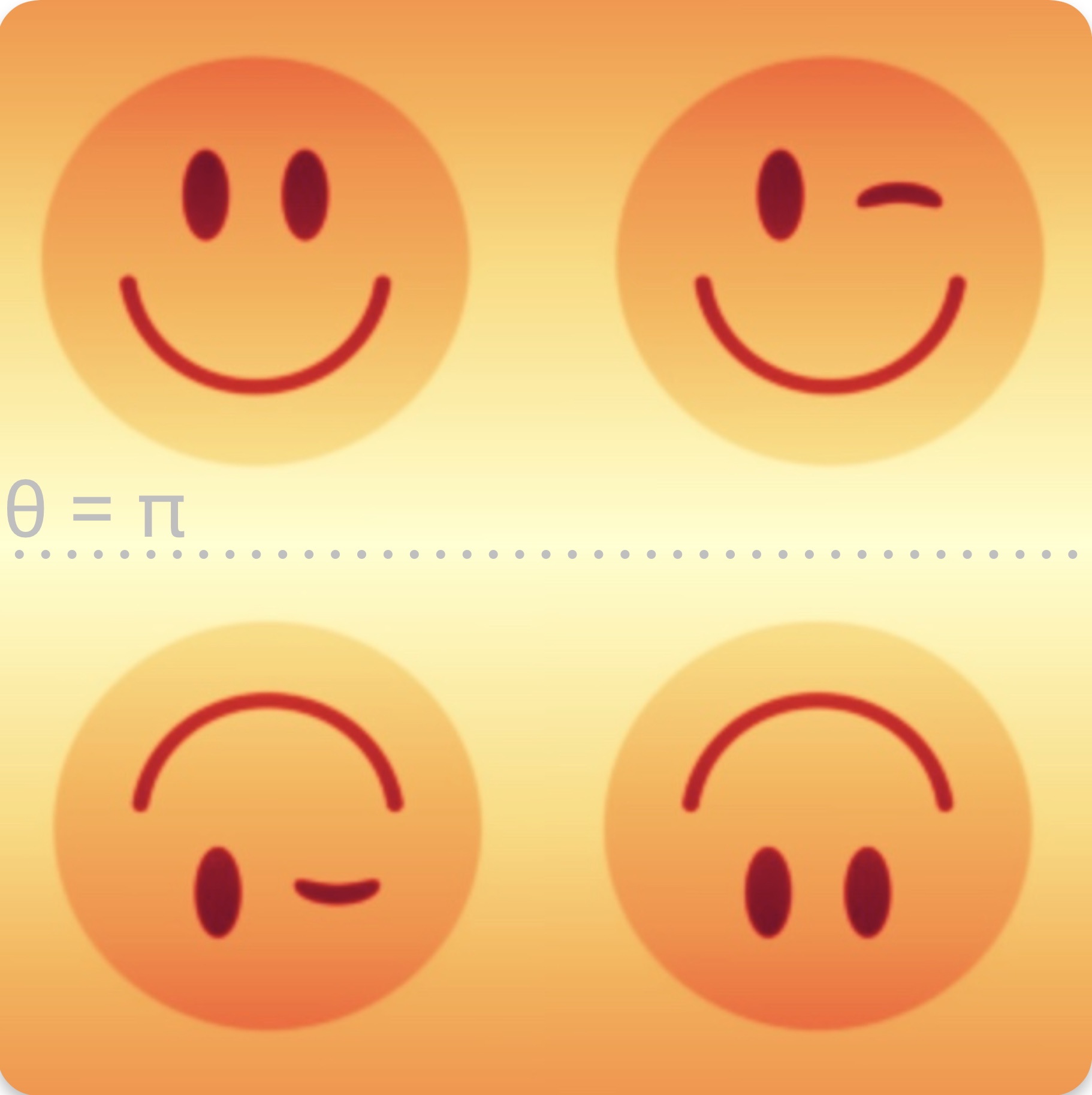
is a “doubling” operation, that extends the range of from to , see Fig. 1. The doubling is performed by extending the meridians across the south pole back up to the north pole. The essential point is that the resulting map, seen as a map on the doubly-periodic torus, has a standard Fourier series with exactly the same Fourier band-limit444This may be seen for example from the well-known Fourier representation of the Wigner -matrices [39, 40], and using the relation . as the spherical harmonic band-limit of the input array . Finally, is simply the standard 2D Fourier transform that produces the Fourier coefficients input to from the doubled map.
The adjoint operator , or the type 1 nuSHT is, by definition,
| (6) |
is a nuFFT of type 1 that produces Fourier frequencies from the input locations and field values. produces from these frequencies a 2D map on the torus. (the adjoint doubling matrix) effectively “folds” this doubled map. The resulting map is -periodic in the -direction, and the -direction goes again from to . The map is then transformed to harmonic coefficients with , an iso-latitude type 1 rSHT.
III Implementation
We discuss the concrete GPU implementation. Readers interested in the CPU equivalent may consult [33].
A GPU is designed to efficiently apply a single instruction on multiple data (SIMD). On the hardware side, it achieves this with Streaming Multiprocessors (SMs) (at the order of 100), that contain a number of simple processors for arithmetic operations (at the order of 100) that execute “warps” of 32 threads in parallel.
On the software side, a GPU accelerated program is executed via a number of threads that are arranged in thread blocks. The GPU is responsible for distributing the thread blocks across the SMs. High throughput is achieved by overloading SMs with many threads as to hide data latency and by ensuring that memory is accessed in multiples of the warp size.
We differentiate between the GPU memory that is “close” to the processor units and can be accessed fast by the device, and host memory, that is managed by the host system of the GPU, and which is generally slow to access by the GPU. We show data transfer benchmarks in Appendix A. Our implementation avoids data transfer and usage of host memory altogether; intermediate results are kept in GPU memory. This is realized by cupy-arrays in combination with a C++-binding nanobind, [41], handily providing a nanobind-cupy interface.
Our implementation of the individual operators , , , and and their adjoints are realised as follows.
For the (adjoint) synthesis () , we use the highly efficient software package SHTns [22], and calculate the SHTs onto a Clenshaw-Curtis (CC) grid. The GPU implementation requires the sample size to be divisible by .
For iso-latitude rings, in order to achieve best efficiency for the Legendre transform part (the part of the transform, which is the critical part), modern top-performing CPU and GPU codes like SHTns use on-the-fly calculation of using efficient recurrence formulas put forward recently [42]. This allows to keep memory usage low: indeed, only the recurrence coefficients that are independent of need to be stored, which requires only memory, the same order as the data. It leaves two dimensions along which to parallelize: and , and requires a sequential loop over to compute the recursively. When is larger than 500 to 1000, this leaves enough parallelization opportunities to efficiently use all of the GPU compute units. The computational complexity stays .
The (adjoint) doubling () is implemented via CUDA, and we write the arrays in a -contiguous memory layout, as required by SHTns to keep high efficiency for the Legendre transform. The computational complexity is .
For the type- and type- nuFFT in -dimensions (, ), we use cufinuFFT [43] in double precision. The nuFFT method works by utilizing the Fourier transform convolution theorem, and interpolation or convolution onto a slightly larger, up-sampled grid. Highly accurate versions use kernels whose error decrease exponentially as a function of the up-sampling factor. The computational complexity (without planning phase) is in 2 dimensions. It is worth mentioning that we use the guru interface to cufinuFFT to initialize the nuFFT plans. The plans allow for repeated and fast transforms, without re-initialization. However, this planning step is the most time consuming operation and is therefore done before calling the functions.
For the FFT operations (type 2) and (type 1), we use the package cupyx [44] and its cuFFT555https://developer.nvidia.com/cufft integration therein. For the type 1 Fourier synthesis, we use double precision accuracy. For the type 2 Fourier synthesis, we use single precision accuracy for , which increases speed at the cost of a negligible decrease in effective accuracy on the final result. The computational complexity is .
FFTs become particularly fast if the prime factorization for the sample size gives many small prime numbers, in the following referred to as a good number. If additional constraints are put on the sample size, good numbers may be more difficult to find, see Appendix B for a discussion and concrete definition.
Ignoring the scaling with accuracy, the overall asymptotic computational complexity (for both type 1 and 2) is,
| (7) | ||||
Here, we assume that the number of uniform and nonuniform points are about the same.
(and ) could be further optimized: and both contain a Fourier transform in -direction, effectively cancelling out each other. Avoiding this reduces to a -dimensional Fourier transform and to a Legendre transformation. This optimization is implemented in the CPU implementation in DUCC. We leave this optimization to a future study for the GPU implementation. We only expect a large speed up for the operator in cunuSHT, which takes about 10 to 20% of the total runtime.
For CMB weak lensing applications, we also provide a pointing routine implemented via CUDA, see Appendix C.
IV Benchmark
We present the scaling and execution time of our implementation. We take as a use case an application in CMB weak lensing [23]. CMB weak lensing describes the deflection of primordial CMB photons by mass fluctuations along the line of sight as they travel through the Universe. These small deflections (their root-mean-square is of the order of a few arcminutes) are large enough to be detectable in CMB sky maps [45, 5, 46]. For some applications, it is necessary to simulate these deflections accurately and efficiently [47, 27, 48].
Owing to the deflections, the CMB intensity field observed at location is the un-deflected field at another location,
| (8) |
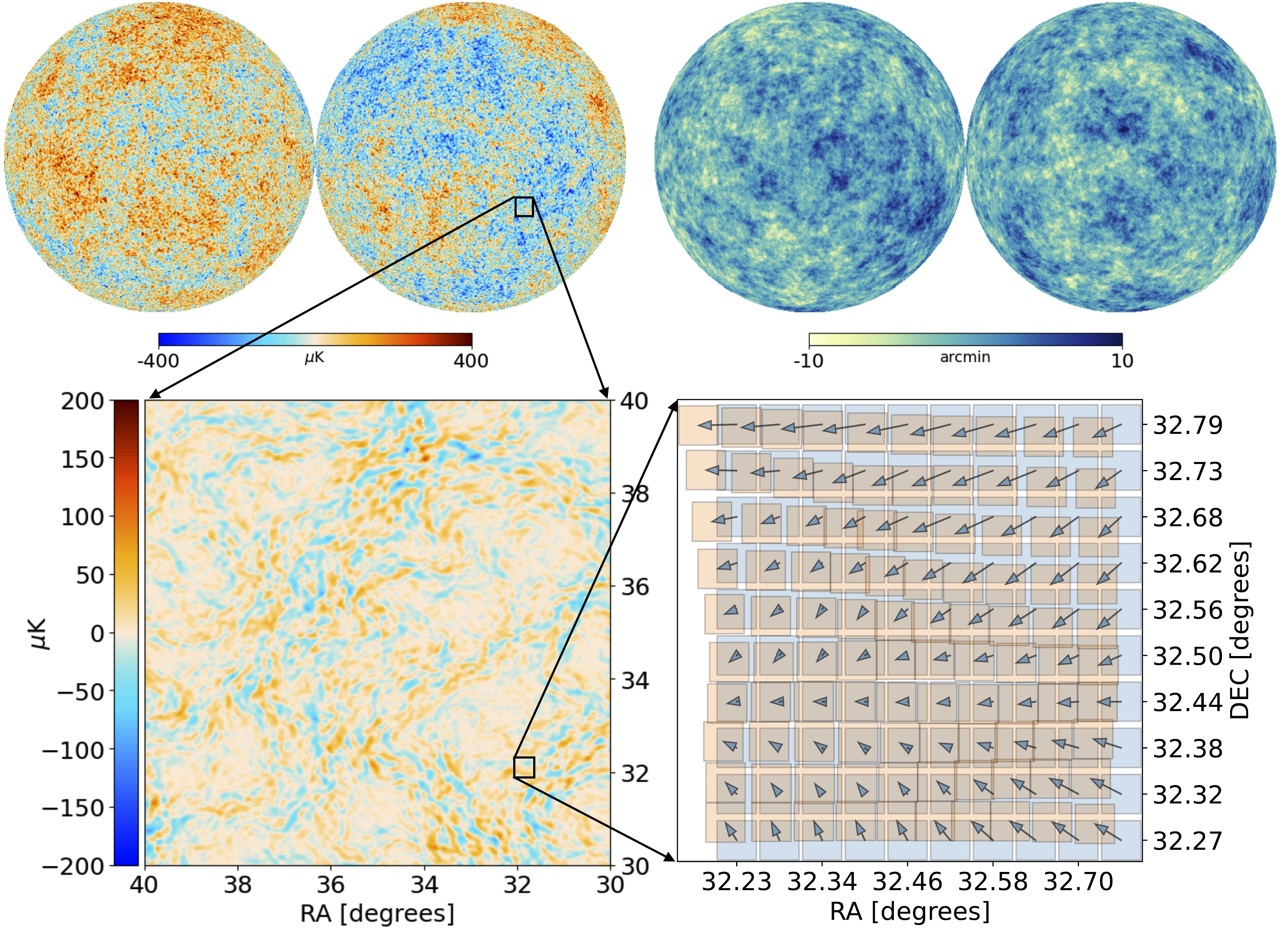
where depends on in a smooth way. Details on how these angles relate to each other are given in Appendix C. For the type-2 nuSHT, the inputs are the set of angles and the spherical harmonic coefficients of the un-deflected field . For type-1, the input are the same set of angles and a set of values of . The set up of our use case is shown in Fig. 2. The top left panel shows the input CMB map, the deflection field is shown on the top right. Both are shown in orthographic projection. The bottom maps show a detail view of degree of the difference between the input and deflected map (left panel) and a detail view of approximately degree (right panel) of the nonuniform point (orange squares) relative to the uniform point locations (blue squares). We use the same setup for the adjoint operation, in which case the deflected map becomes the input, and the result becomes the adjoint SHT coefficients.
Benchmarks are run on an NVIDIA A-100 GPU with GB of memory and an Intel Xeon Gold 8358 Processor with 32 cores. We set the number of threads to for the CPU benchmarks. If not stated otherwise, we choose the following parameters (that mostly affect the nuFFT): an up-sampling factor of to reduce the memory usage at a small price of increased computation time666This somewhat low up-sampling factor reduces the minimal possible accuracy, in double precision, to due to its dependence on the size of the up-sampled grid, but can easily be changed by the user, if needed., a gpu_method utilizing the hybrid scheme, called shared memory, and the default kernel evaluation method. The resulting map (or input map in the case of the adjoint) is calculated on a Gauss-Legendre grid.
With this implementation, we can solve problem sizes of up to on an A-100 with GB, by using the pre-computed nuFFT plans and keeping all necessary intermediate results in memory.
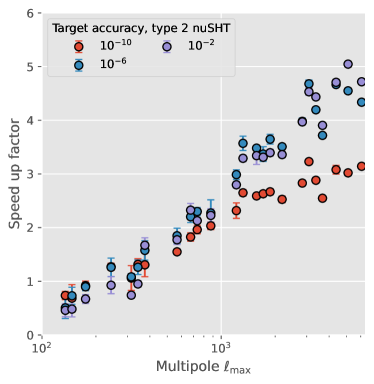
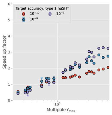
Fig. 3 shows the speed up of the GPU algorithm compared to the CPU as a function of for different accuracies. The left panel shows the evaluation of Eq. (5), the right panel shows Eq. (6). The variance from runs is indicated by error bars.
For type 2 nuSHT, we reach a speed up between 1 and 5 times for single precision and 1 to 3 times for double precision, with the speed up increasing with increasing . This increase is expected due to better parallelizability for GPUs for higher . The speed up is mostly independent of the target accuracy, with the smallest accuracies tending to perform better. For type 1 nuSHT, we find lower speed up factors, which may indicate further improvements. However, type 1 directions are generally expected to perform worse on the GPU due to the shear amount of threads that have to be written concurrently to the same memory location. Nevertheless, the GPU code either performs almost as good as the CPU code (small ), or better by a factor of up to for large problem sizes. For high , the speed up depends on the accuracy, with lower accuracies performing better. For double precision (), the speed up is diminished due to the double precision penalty that we pay in our implementation.
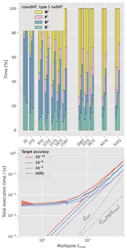
We can get a better understanding of the resulting speed up factors by looking at the time spent on each of the operators on the GPU. This breakdown is shown in the top panels of Fig. 4 for the type 2 (left panel) and type 1 (right panel) nuSHT, as a function of for different accuracies. The respective total execution times are shown in the bottom panels together with the empirically fitted computational complexity model, Eq. (D1). At the top panels, for each problem size , each bar represents a benchmark with an accuracy of (from left to right) , , . Each bar represent the mean over 5 runs. For small problem sizes, doubling dominates and becomes almost negligible for large . only takes about 20% of the execution time for large , even though it has the worst asymptotic computational complexity. This highlights the quality of the rSHT implementation by SHTns.
The choice of accuracy has an impact on the total execution time, as seen in the bottom panels of Fig. 4. The highest accuracy (, red line) takes at most twice as long compared to the low accuracy (, purple line). Our results suggests that improvements in might be possible: due to FFT being in principle a bandwidth limited routine, we would expect the execution time of to be comparable to that of , and only a fraction of that of . For type 1 (right column), the total execution time overall takes longer. The breakdown shows that for the low and intermediate accuracy cases, less time is spend in the call. This is a consequence of our use of single precision arithmetic FFTs for the case, which, as mentioned before, is possible for the type 1 nuSHT.
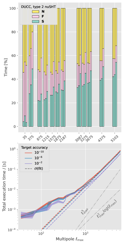
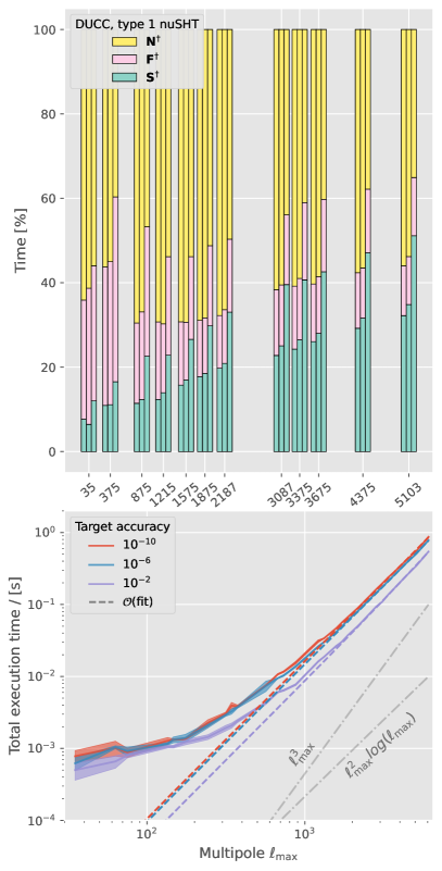
It is interesting to compare this breakdown to the CPU implementation of DUCC. While we cannot expect both breakdowns to be exactly the same due to the different nature of the hardware, large differences may imply possible improvements. Fig. 5 shows the computation time of the CPU implementation of DUCC for the type 2 nuSHT (left column) and type 1 nuSHT (right column) as a function of for different accuracies. Looking at the top left panel, we see that increases with increasing , as expected from its scaling. The bottom panel of the left figure shows that the total execution time of the high-accuracy run is at most twice as long as the low accuracy one.
Many optimizations have gone into DUCC’s and SHTns’s SHT routines (, ) over the years and it is safe to assume that they are close to optimal. Comparing the breakdown of the CPU and GPU implementation for (green bars) shows that DUCC spends more than twice as long with this operator. This hints to potential sub-optimalities in the implementations of the GPU operators. This also becomes apparent when we look at the operator (and ). The scaling with the problem size is much more pronounced for the GPU code.
Fig. 6 shows the effective accuracy as a function of target accuracy for both CPU and GPU. The effective accuracy is calculated by solving Eq. (3) in a brute-force manner (giving us the values ) and comparing it against Eq. (5) (giving us the values ),
| (9) |
with
| (10) |
We choose random points on the sphere, giving us good sampling across the full sphere, and a sufficiently low variance on .
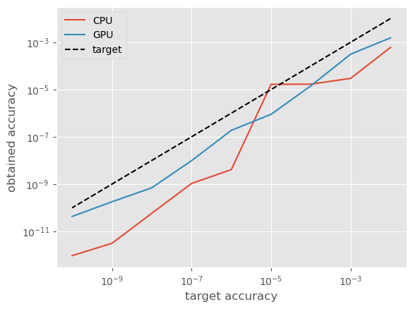
Both algorithms achieve good effective accuracies, with the CPU code being more conservative. For the GPU implementation, we note that only low effective accuracies, , can be achieved when nuFFT is executed in single precision. When an accuracy of is desired, a single precision nuFFT evaluation is thus insufficient. We find that executing and in double precision solves this. There is an associated penalty in efficiency due to the double precision calculations being approximately twice as slow. The nuFFT implementation in DUCC circumvents this by allowing for double precision accuracy on the pointing and intermediate results while using single precision accuracy on the Fourier coefficients, hereby reducing the execution time for single precision accuracies.
V Conclusion
We presented cunuSHT, a GPU accelerated implementation of the spherical harmonic transform on arbitrary pixelization that is, to our knowledge, the first of its kind to achieve faster execution when compared against CPU based algorithms. cunuSHT achieves machine precision accuracy by transforming the problem of interpolating on the sphere into a problem of computing a nonuniform fast Fourier transform on the torus. Comparing our implementation executed on an A-100 to the fastest available CPU implementations to date running on a single Intel Xeon Gold 8358 Processor with cores, we find that our implementation is up to times faster. We used highly efficient, publicly available packages that are well tested and robust: SHTns for rSHTs, cufinuFFT for nuFFTs. We found that, although it has the highest asymptotic complexity, the high-quality rSHT implemented in SHTns is not the bottleneck. Our code does not require intermediate transfers between host and device, allowing it to be incorporated within larger GPU-based algorithms. Many applications in cosmology that we have in mind typically require spin- to transforms. We thus plan to extend this package to spin- transforms in the near future. There are, in principle, no obstacles to the generalization to spin- by implementing the corresponding Wigner- transform.
cunuSHT is a general purpose package distributed via pypi, and also works on standard pixelization schemes such as HEALPix, and can also perform rSHTs. Demonstrations of our package on GitHub present how to integrate it into exisiting pipelines.
Acknowledgment
The authors thank Alex Barnett for helpful discussions about nuFFT, Lehman Garrison for help on the cupy-nanobind implementation, and Libin Lu for general discussion and upgrades to cufinuFFT. This work is supported by the Research Analyst grant from the Simons Foundation and the computing resources of the Flatiron Institute. The Flatiron Institute is supported by the Simons Foundation. SB and JC acknowledges support from a SNSF Eccellenza Professorial Fellowship (No. 186879).
References
- Hivon et al. [2002] E. Hivon, K. M. Górski, C. B. Netterfield, B. P. Crill, S. Prunet, and F. Hansen, MASTER of the Cosmic Microwave Background Anisotropy Power Spectrum: A Fast Method for Statistical Analysis of Large and Complex Cosmic Microwave Background Data Sets, Astrophys. J. 567, 2 (2002), arXiv:astro-ph/0105302 [astro-ph] .
- Aghanim et al. [2020a] N. Aghanim et al. (Planck), Planck 2018 results. VIII. Gravitational lensing, Astron. Astrophys. 641, A8 (2020a), arXiv:1807.06210 [astro-ph.CO] .
- Ade et al. [2021] P. A. R. Ade et al. (SPTpol, BICEP, Keck), A demonstration of improved constraints on primordial gravitational waves with delensing, Phys. Rev. D 103, 022004 (2021), arXiv:2011.08163 [astro-ph.CO] .
- Ade et al. [2018] P. A. R. Ade et al. (BICEP2, Keck Array), BICEP2 / Keck Array X: Constraints on Primordial Gravitational Waves using Planck, WMAP, and New BICEP2/Keck Observations through the 2015 Season, Phys. Rev. Lett. 121, 221301 (2018), arXiv:1810.05216 [astro-ph.CO] .
- Qu et al. [2024] F. J. Qu et al. (ACT), The Atacama Cosmology Telescope: A Measurement of the DR6 CMB Lensing Power Spectrum and Its Implications for Structure Growth, Astrophys. J. 962, 112 (2024), arXiv:2304.05202 [astro-ph.CO] .
- Hanany et al. [2019] S. Hanany et al. (NASA PICO), PICO: Probe of Inflation and Cosmic Origins, (2019), arXiv:1902.10541 [astro-ph.IM] .
- Scharf and Lahav [1993] C. A. Scharf and O. Lahav, Spherical Harmonic Analysis of the 2-JANSKY IRAS Galaxy Redshift Survey, MNRAS 264, 439 (1993).
- Hikage et al. [2011] C. Hikage, M. Takada, T. Hamana, and D. Spergel, Shear power spectrum reconstruction using the pseudo-spectrum method, MNRAS 412, 65 (2011), arXiv:1004.3542 [astro-ph.CO] .
- Deppe et al. [2024] N. Deppe, W. Throwe, L. E. Kidder, N. L. Vu, K. C. Nelli, C. Armaza, M. S. Bonilla, F. Hébert, Y. Kim, P. Kumar, G. Lovelace, A. Macedo, J. Moxon, E. O’Shea, H. P. Pfeiffer, M. A. Scheel, S. A. Teukolsky, N. A. Wittek, et al., SpECTRE v2024.06.18, 10.5281/zenodo.12098412 (2024).
- Wedi et al. [2013] N. P. Wedi, M. Hamrud, and G. Mozdzynski, A fast spherical harmonics transform for global nwp and climate models, Monthly Weather Review 141, 3450 (2013).
- Brun and Rempel [2009] A. S. Brun and M. Rempel, Large Scale Flows in the Solar Convection Zone, "Space Science Reviews" 144, 151 (2009).
- Browning et al. [1989] G. L. Browning, J. J. Hack, and P. N. Swarztrauber, A comparison of three numerical methods for solving differential equations on the sphere, Monthly Weather Review 117, 1058 (1989).
- Driscoll and Healy [1994] J. Driscoll and D. Healy, Computing fourier transforms and convolutions on the 2-sphere, Advances in Applied Mathematics 15, 202 (1994).
- Potts et al. [1998a] D. Potts, G. Steidl, and M. Tasche, Fast and stable algorithms for discrete spherical fourier transforms, Linear Algebra and its Applications 275-276, 433 (1998a), proceedings of the Sixth Conference of the International Linear Algebra Society.
- Potts et al. [1998b] D. Potts, G. Steifdl, and M. Tasche, Fast algorithms for discrete polynomial transforms, Mathematics of Computation 67 (1998b).
- Keiner et al. [2009] J. Keiner, S. Kunis, and D. Potts, Using NFFT3 - a software library for various nonequispaced fast Fourier transforms, ACM Trans. Math. Software 36, Article 19, 1 (2009).
- Seljebotn [2012] D. S. Seljebotn, Wavemoth-fast spherical harmonic transforms by butterfly matrix compression, The Astrophysical Journal Supplement Series 199, 5 (2012).
- Hale and Townsend [2015] N. Hale and A. Townsend, A fast FFT-based discrete Legendre transform, IMA Journal of Numerical Analysis 36, 1670 (2015), https://academic.oup.com/imajna/article-pdf/36/4/1670/7920439/drv060.pdf .
- Slevinsky [2019] R. M. Slevinsky, Fast and backward stable transforms between spherical harmonic expansions and bivariate fourier series, Applied and Computational Harmonic Analysis 47, 585 (2019).
- Yin et al. [2019] F. Yin, J. Wu, J. Song, and J. Yang, A high accurate and stable legendre transform based on block partitioning and butterfly algorithm for nwp, Mathematics 7, 10.3390/math7100966 (2019).
- Reinecke and Seljebotn [2013] M. Reinecke and D. S. Seljebotn, Libsharp - spherical harmonic transforms revisited, Astronomy & Astrophysics 554, A112 (2013).
- Schaeffer [2012] N. Schaeffer, Efficient spherical harmonic transforms aimed at pseudospectral numerical simulations, Geochemistry 14, 751 (2012).
- Lewis and Challinor [2006] A. Lewis and A. Challinor, Weak gravitational lensing of the cmb, Phys. Rept. 429, 1 (2006), arXiv:astro-ph/0601594 [astro-ph] .
- Fabbian et al. [2018] G. Fabbian, M. Calabrese, and C. Carbone, Cmb weak-lensing beyond the born approximation: a numerical approach, Journal of Cosmology and Astroparticle Physics 2018 (02), 050–050.
- Ferlito et al. [2024] F. Ferlito, C. T. Davies, V. Springel, M. Reinecke, A. Greco, A. M. Delgado, S. D. M. White, C. Hernández-Aguayo, S. Bose, and L. Hernquist, Ray-tracing vs. born approximation in full-sky weak lensing simulations of the millenniumtng project (2024), arXiv:2406.08540 .
- Wandelt et al. [2004] B. D. Wandelt, D. L. Larson, and A. Lakshminarayanan, Global, exact cosmic microwave background data analysis using Gibbs sampling, Phys. Rev. D 70, 083511 (2004), arXiv:astro-ph/0310080 [astro-ph] .
- Carron and Lewis [2017] J. Carron and A. Lewis, Maximum a posteriori CMB lensing reconstruction, Phys. Rev. D 96, 063510 (2017), arXiv:1704.08230 [astro-ph.CO] .
- Lewis [2005] A. Lewis, Lensed CMB simulation and parameter estimation, Phys. Rev. D71, 083008 (2005), arXiv:astro-ph/0502469 [astro-ph] .
- Næss and Louis [2013] S. K. Næss and T. Louis, Lensing simulations by taylor expansion — not so inefficient after all, Journal of Cosmology and Astroparticle Physics 2013 (09), 001–001.
- Basak et al. [2008] S. Basak, S. Prunet, and K. Benabed, Simulating weak lensing on cmb maps, (2008), arXiv:0811.1677 [astro-ph] .
- Merilees [1973] P. E. Merilees, The pseudospectral approximation applied to the shallow water equations on a sphere, Atmosphere 11, 13 (1973), https://doi.org/10.1080/00046973.1973.9648342 .
- Townsend et al. [2016] A. Townsend, H. Wilber, and G. B. Wright, Computing with Functions in Spherical and Polar Geometries I. The Sphere, SIAM Journal on Scientific Computing 38, C403 (2016), arXiv:1510.08094 [math.NA] .
- Reinecke et al. [2023] M. Reinecke, S. Belkner, and J. Carron, Improved cosmic microwave background (de-)lensing using general spherical harmonic transforms, Astron. Astrophys. 678, A165 (2023), arXiv:2304.10431 [astro-ph.CO] .
- Hupca et al. [2012] I. O. Hupca, J. Falcou, L. Grigori, and R. Stompor, Spherical harmonic transform with gpus, in Lecture Notes in Computer Science (Springer Berlin Heidelberg, 2012) p. 355–366.
- Szydlarski et al. [2013] M. Szydlarski, P. Esterie, J. Falcou, L. Grigori, and R. Stompor, Parallel spherical harmonic transforms on heterogeneous architectures (gpus/multi-core cpus), (2013), arXiv:1106.0159 [cs.DC] .
- Price and McEwen [2024] M. A. Price and J. D. McEwen, Differentiable and accelerated spherical harmonic and wigner transforms, Journal of Computational Physics 510, 113109 (2024).
- Baleato Lizancos and White [2024] A. Baleato Lizancos and M. White, Harmonic analysis of discrete tracers of large-scale structure, JCAP 05, 010, arXiv:2312.12285 [astro-ph.CO] .
- Barnett et al. [2019] A. H. Barnett, J. Magland, and L. af Klinteberg, A Parallel Nonuniform Fast Fourier Transform Library Based on an “Exponential of Semicircle” Kernel, SIAM Journal on Scientific Computing 41, C479 (2019), arXiv:1808.06736 [math.NA] .
- Risbo [1996] T. Risbo, Fourier transform summation of legendre series and d-functions, Journal of Geodesy 70, 383 (1996).
- Huffenberger and Wandelt [2010] K. M. Huffenberger and B. D. Wandelt, Fast and Exact Spin-s Spherical Harmonic Transforms, Astrophys. J. Suppl. 189, 255 (2010), arXiv:1007.3514 [astro-ph.IM] .
- Jakob [2022] W. Jakob, nanobind: tiny and efficient c++/python bindings (2022), https://github.com/wjakob/nanobind.
- ISHIOKA [2018] K. ISHIOKA, A new recurrence formula for efficient computation of spherical harmonic transform, Journal of the Meteorological Society of Japan. Ser. II 96, 241 (2018).
- hsuan Shih et al. [2021] Y. hsuan Shih, G. Wright, J. Andén, J. Blaschke, and A. H. Barnett, cufinufft: a load-balanced gpu library for general-purpose nonuniform ffts, 2021 IEEE International Parallel and Distributed Processing Symposium Workshops (IPDPSW) , 688 (2021).
- Okuta et al. [2017] R. Okuta, Y. Unno, D. Nishino, S. Hido, and C. Loomis, Cupy: A numpy-compatible library for nvidia gpu calculations, in Proceedings of Workshop on Machine Learning Systems (LearningSys) in The Thirty-first Annual Conference on Neural Information Processing Systems (NIPS) (2017).
- Aghanim et al. [2020b] N. Aghanim et al. (Planck), Planck 2018 results. VIII. Gravitational lensing, Astron. Astrophys. 641, A8 (2020b), arXiv:1807.06210 [astro-ph.CO] .
- Pan et al. [2023] Z. Pan et al. (SPT), Measurement of gravitational lensing of the cosmic microwave background using SPT-3G 2018 data, Phys. Rev. D 108, 122005 (2023), arXiv:2308.11608 [astro-ph.CO] .
- Hirata and Seljak [2003] C. M. Hirata and U. Seljak, Reconstruction of lensing from the cosmic microwave background polarization, Phys. Rev. D68, 083002 (2003), arXiv:astro-ph/0306354 [astro-ph] .
- Belkner et al. [2024] S. Belkner, J. Carron, L. Legrand, C. Umiltà, C. Pryke, and C. Bischoff (CMB-S4), CMB-S4: Iterative Internal Delensing and r Constraints, Astrophys. J. 964, 148 (2024), arXiv:2310.06729 [astro-ph.CO] .
Appendix A Data Transfer
All benchmarks are done without measuring the time to transfer the data to device and back. This can be a large part of the overall computation and should be avoided, as is shown in Fig. A1 for different problem sizes. We note here that cunuSHT provides means to keep everything on the GPU without having to transfer the data. Thus, these transfer times can in principle be avoided.
Appendix B Good numbers
For fast Fourier transforms, execution time depends strongly on the largest prime factor of the transform length; the smaller it is, the better. Luckily enough, many good numbers for CPU algorithms exist. Assuming Clenshaw-Curtis quadrature, the constraint on the number of rings to sufficiently sample a map with band limit is . Therefore, after applying the double Fourier sphere method, we must have at least samples, and we are free to choose an arbitrarily larger number which happens to be a good FFT size. For the GPU algorithm, however, there is a caveat: due to the additional constraint on to be divisible by for the rSHT operation, the selection of good numbers is reduced. While there are still good numbers for FFT satisfying both constraints, they are sparser. The full list of that are multiples of 4 up to for which can be factored into primes up to 11 is 4, 8, 12, 16, 28, 36, 56, 64, 76, 100, 136, 148, 176, 232, 244, 276, 316, 344, 364, 376, 496, 540, 568, 676, 736, 848, 876, 892, 1156, 1216, 1324, 1332, 1376, 1576, 1716, 1816, 1876, 2080, 2188, 2476, 2696, 2836, 3088, 3268, 3376, 3676, 4236, 4376, 4456, 4852, 5104, 5776, 6076, 6616, 6656, 6876, 7204, 7624, 7876, 8020, 8576, 9076, 9376. The numbers with the highest prime factor being 11 are highlighted with an underline as efficient calculation of cunuSHT only applies to the CPU code here.
One way to enlarge this list could be for example by using a Fejér grid as intermediate grid, as opposed to the currently used Clenshaw-Curtis grid. This would effectively reduce the number of required samples to after doubling, resulting in a much wider choice of sample sizes that are also good FFT lengths. Hence restrictions on the number of good numbers are expected to go away in the future.
Appendix C CMB weak lensing pointing
Let and form the right-handed unit basis vectors at the point on the sphere parametrized by (so, the components of are ). In our benchmark CMB lensing application, the deflected positions that define the angles and at which the CMB field must be evaluated are given by,
| (C1) |
where , and and form the gradient of the lensing potential ,
| (C2) |
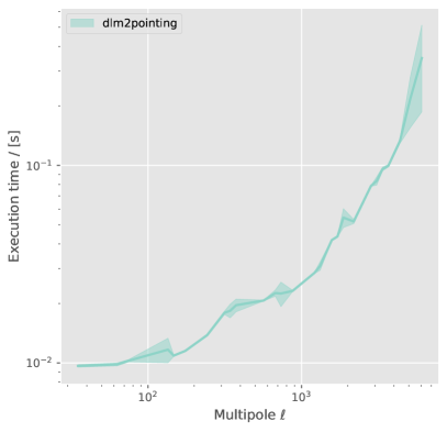
cunuSHT first obtains and from this equation using SHTns. Then, threading across each ring, we solve for in Eq. (C1) on the fly. A benchmark as a function of is shown in Fig. C1.
Appendix D Computational complexity
Table D1 shows the results for the empirical fit of the type 2 and type 1 nuSHT computational complexity models,
| (D1) |
with the normalization for the unknown prefactors. Compared to Eq. (7) we only account for the terms with the largest complexities. The fits are shown in Fig. 3, Fig. 4, and Fig. 5.
| type 2 | Target acc. | ||
|---|---|---|---|
| CPU | |||
| GPU | |||
| type 1 | Target acc. | ||
| CPU | |||
| GPU | |||
Appendix E Code examples
The following code block shows a minimum working example for calculating a type 2 and type 1 nuSHT on the GPU for SHT coefficients alm that are deflected by a deflection field dlm_scaled, for an accuracy of epsilon and band limit lmax. Both routines will set up the plans, so that the actual nusht2dX() call may be called repeatedly. ⬇ 1import cunusht as cu 2 3lenjob_geominfo = (’gl’,{’lmax’: lmax}) 4kwargs = { 5 ’geominfo_deflection’: lenjob_geominfo, 6 ’epsilon’: epsilon, 7 ’nuFFTtype’: 2, 8} 9t = cu.get_transformer(backend=’GPU’)(**kwargs) 10ptg = t.dlm2pointing(dlm_scaled) 11lenmap = t.nusht2d2(alm, ptg, lmax, lenmap) ⬇ 1import cunusht as cu 2 3lenjob_geominfo = (’gl’,{’lmax’: lmax}) 4kwargs = { 5 ’geominfo_deflection’: lenjob_geominfo, 6 ’epsilon’: epsilon, 7 ’nuFFTtype’: 1, 8} 9t = cu.get_transformer(backend=’GPU’)(**kwargs) 10ptg = t.dlm2pointing(dlm_scaled) 11alm = t.nusht2d1(alm, ptg, lmax, lenmap)