DeciMamba: Exploring the Length Extrapolation Potential of Mamba

Abstract

Long-range sequence processing poses a significant challenge for Transformers due to their quadratic complexity in input length. A promising alternative is Mamba, which demonstrates high performance and achieves Transformer-level capabilities while requiring substantially fewer computational resources. In this paper we explore the length-generalization capabilities of Mamba, which we find to be relatively limited. Through a series of visualizations and analyses we identify that the limitations arise from a restricted effective receptive field, dictated by the sequence length used during training. To address this constraint, we introduce DeciMamba, a context-extension method specifically designed for Mamba. This mechanism, built on top of a hidden filtering mechanism embedded within the S6 layer, enables the trained model to extrapolate well even without additional training. Empirical experiments over real-world long-range NLP tasks show that DeciMamba can extrapolate to context lengths that are 25x times longer than the ones seen during training, and does so without utilizing additional computational resources. We will release our code and models.

https://github.com/assafbk/DeciMamba

DeciMamba: Exploring the Length Extrapolation Potential of Mamba

Assaf Ben-Kish¹   Itamar Zimerman¹   Shady Abu-Hussein¹ Nadav Cohen¹   Amir Globerson^1,2   Lior Wolf¹   Raja Giryes^{1 1}Tel Aviv University     ²Google Research

1 Introduction

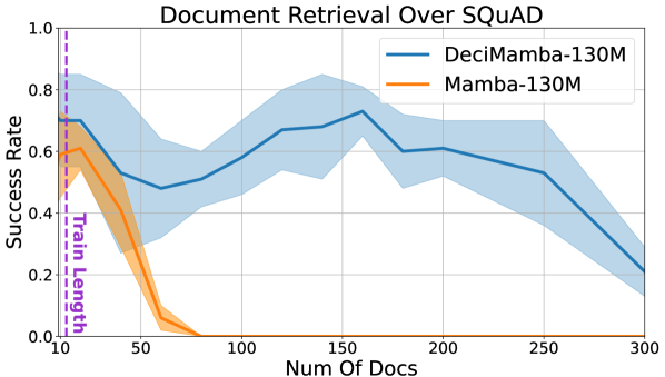
Figure 1: Document Retrieval Over SQuAD. We present a novel decimation mechanism tailored for Mamba, enabling it to process sequences that are x25 times longer than the ones seen during training. The purple line shows the training sequences length. Results are shown for DeciMamba-130M.

Lengthy sequences, which can span up to millions of tokens, are common in real-world applications including long books, high-resolution video and audio signals, and genomic data. Consequently, developing Deep Learning (DL) sequence models capable of effectively managing long contexts is a critical objective. Transformers Vaswani et al. (2017), despite their current dominance in general DL tasks, still face challenges in processing long sequences. Specifically, their quadratic complexity in sequence length makes them computationally demanding, restricting the ability to train them over long sequences and very large datasets.

In recent years, substantial efforts have been made in order to tackle this challenge. The most significant advancements include efficient implementations that increase the model’s context length during training Dao et al. (2022); Liu et al. (2023), and context-extension methods Chen et al. (2023b); Peng et al. (2023b) designed to effectively expand the context after training. However, recent studies suggest that long-range processing is still an unresolved problem Li et al. (2024); Liu et al. (2024a).

One promising approach in this domain is the development of attention-free networks with sub-quadratic complexity, which can be trained more effectively over long sequences. In a recent line of work Gu et al. (2021b, a); Gupta et al. (2022), the family of state-space layers has been introduced. These layers can be seen as theoretically grounded linear RNNs that can be efficiently computed in parallel via convolutions, thanks to a closed-form formulation of their linear recurrent rule. A recent advancement by Gu and Dao (2023) presented Mamba, which builds on top of an expressive variant of SSMs called Selective State-Space Layers (S6). These layers match or exceed the performance of Transformers in several domains, such as NLP Pióro et al. (2024); Wang et al. (2024), image classification Zhu et al. (2024); Liu et al. (2024b), audio processing Shams et al. (2024), genomic data Schiff et al. (2024), and more.

In this paper, we first explore the length-generalization abilities of Mamba and identify that they are relatively limited. Although Mamba layers are theoretically capable of capturing global interactions at the layer level, through a series of visualizations, analyses, and empirical measures, we show that the main barrier preventing Mamba from extrapolating is its implicit bias towards a limited effective receptive field (ERF), which is bounded primarily by the sequence length used during training. Secondly, based on the assumption that long-context data is usually sparse, we present DeciMamba, the first context-extension method specifically designed for S6. Our method relies on a dynamic data-dependent pooling method that utilizes a hidden filtering mechanism intrinsic to the Mamba layer. We leverage this mechanism to introduce a global compression operator, which expands Mamba’s ERF by discarding un-important tokens before each S6 layer. Our method significantly increases the effective context length of Mamba by several orders of magnitude while requiring a smaller computational budget.

Our main contributions encompass the following three aspects: (i) identify that Mamba has limited length-extrapolation capabilities, (ii) recognize via a series of visualizations, analyses, and empirical measures that although Mamba can theoretically capture global interactions via the recurrent state, its limited ERF prevents significant length-extrapolation. (iii) Building on this insight, we introduce DeciMamba, the first context-extension technique specifically designed for Mamba models. This approach leverages an existing filtering mechanism embedded within the S6 layer. As illustrated in Fig. 9, our method effectively enhances Mamba’s length-extrapolation abilities by up to eightfold, and is applicable to real-world long-context NLP tasks, as demonstrated in Fig. 1.

2 Preliminaries

In this section, the scientific context for discussion of long-range models is described and the necessary terminology and symbols are provided. Such models evolve in two main directions: (i) first, by adapting transformers, the most dominant architecture today, to be more suitable for such tasks, or, alternatively, (ii) by developing architectures with sub-quadratic complexity in sequence length. Several modern examples include Hyena Poli et al. (2023), RWKV Peng et al. (2023a), Hawk De et al. (2024), xLSTM Beck et al. (2024), and Mamba, the latter being the focus of our paper.

Mamba. Given an input sequence $U=(u_{1},u_{2},\ldots,u_{L})\in\mathbb{R}^{L\times d}$ of length $L$ such that $u_{i}\in\mathbb{R}^{d}$, a Mamba block with $d$ channels is built on top of the S6 layer via the following formula:

$$G=\mathrm{\sigma}(\text{Linear}(U)),\quad X=\text{Conv1D}(\text{Linear}(U)),$$ (1)

$$Y=S6(X),\quad O=Y\otimes G$$ (2)

where $G$ represents the gate branch, $\otimes$ is elementwise multiplication, $\mathbf{\sigma}$ is the SILU activation, Linear and Conv1D are standard linear projection and 1-dimensional convolution layers. The S6 layer is based on a time-variant SSM, which can be elaborated by the following recurrent rule:

$$\vspace{-3pt}h_{t}=\bar{A}_{t}h_{t-1}+\bar{B}_{t}x_{t},\quad y_{t}=C_{t}h_{t}\vspace{-3pt}$$ (3)

Where $X=(x_{1},x_{2},\ldots,x_{L})$ is the input sequence of a representative channel, $\bar{A}_{t}\in\mathbb{R}^{N\times N}$, $\bar{B}_{t}\in\mathbb{R}^{N\times 1}$, and $C_{t}\in\mathbb{R}^{1\times N}$ are the system, input, and output discrete time-variant matrices, respectively. S6 conditions the discrete time-variant matrices based on the input as follows:

$$\Delta_{t}=\textit{Sft}(S_{\Delta}X_{t}),\quad B_{t}=S_{B}X_{t},\quad C_{t}=(S_{C}X_{t})^{T}$$ (4)

$$\bar{A}_{t}=\exp(A\Delta_{t}),\quad\bar{B}_{t}=B_{t}\Delta_{t}$$ (5)

such that $\Delta_{t}$ is the discretization step, Sft represents the softplus function, and $S_{\Delta},S_{B},S_{C}$ are linear projection layers. Ali et al. (2024) demonstrated that S6 layers, similar to attention models, can be interpreted as data-controlled linear operators. Specifically, the S6 layer computation can be represented using the following linear operator $\alpha$, controlled by the input (via Eq. 4 and 5):

$$\vspace{-3pt}Y=\alpha X,\quad\alpha_{i,j}=C_{i}\Big{(}\Pi_{k=j+1}^{i}\bar{A}_{k}\Big{)}\bar{B}_{j}$$ (6)

$$\begin{bmatrix}y_{1}\\ y_{2}\\ \vdots\\ y_{L}\\ \end{bmatrix}=\begin{bmatrix}C_{1}\bar{B}_{1}&0&\cdots&0\\ C_{2}\bar{A}_{2}\bar{B}_{1}&C_{2}\bar{B}_{2}&\cdots&0\\ \vdots&\vdots&\ddots&0\\ C_{L}\Pi_{k=2}^{L}\bar{A}_{k}\bar{B}_{1}\quad&C_{L}\Pi_{k=3}^{L}\bar{A}_{k}\bar{B}_{2}\quad&\cdots\quad&C_{L}\bar{B}_{L}\end{bmatrix}\begin{bmatrix}x_{1}\\ x_{2}\\ \vdots\\ x_{L}\\ \end{bmatrix}$$ (7)

In this formulation, each output $y_{i}$ is a weighted sum of all inputs, where the ‘attention weights’ of all inputs $x_{j}$, i.e., the set $\{\alpha_{i,j}\}_{j=1}^{L}$, is data-driven. We utilize this perspective to further investigate the effective receptive field of Mamba layers.

Context Extension & Length Extrapolation. Over the years, several methods have been proposed to enhance the effective context length of transformers and improve their ability to extrapolate over longer sequences. Traditionally, length generalization is closely related to positional encoding. Pioneering work in the domain, introduced by Press et al. (2021), demonstrates that models built on top of original sinusoidal, rotary Su et al. (2024), and T5 bias Raffel et al. (2020) positional encoding have poor length generalization abilities. It proposes Alibi, which mitigates this issue by promoting locality through the incorporation of distance-based linear biases into the attention matrix. A counter-intuitive study was conducted by Kazemnejad et al. (2024), which shows that transformers without positional encoding (NoPE) exhibit better length extrapolation capabilities in downstream tasks. Two more promising approaches are the very recent CoPE Golovneva et al. (2024), which utilizes context-aware positional encoding, and post-training positional interpolation Peng et al. (2023b); Chen et al. (2023a).

Alternatively, a recent direction involves architectural modifications to pre-trained models followed by short fine-tuning. Such works include LongLora Chen et al. (2023b), which proposes shifted sparse attention, and Landmark Attention Mohtashami and Jaggi (2023), which applies attention in chunks and inserts global unique tokens into the input sequences between those chunks. Our method can be considered an application of this approach to Mamba models, rather than to traditional transformers. More related work is in App. B.

We note that in order to assess the long range performance of the model, in our experiments we measure perplexity only on the farthest labels of the context window, causing the perplexity values to be larger than their typical values (usually, all labels in the context window are aggregated).

3 Extrapolation Limitations of Mamba

In this section we explore the length-generalization capabilities of Mamba models. Specifically, we assess the effective receptive field (ERF) of S6 layers, a phenomenon that leads to poor information propagation when processing sequences that are longer than the ones trained on.

To investigate why Mamba fails at long sequence extrapolation we visualize Mamba’s hidden attention (Eq. 6, 7). In Fig. 2 we display the attention matrices of Mamba-130M after training it on the Passkey Retrieval task (Sec. 5) with a sequence length of 2K. We record the data for the matrices in layer 17, while evaluating sequences of length 2K and 16K. Notice that while the attention maps are very dense for the 2K sequence inference, the attention maps for the 16K sequence are much more sparse, and their elements vanish as we move towards the lower rows. This exhibits a limited effective receptive field (ERF), as information from the first tokens in the sequence does not propagate to the final tokens in the output sequence.

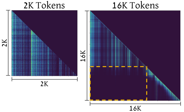
Figure 2: ERF Detected by the Mamba Attention Matrix (Eq. 7). We feed Mamba-130m with two sequences of different lengths, 2K and 16K, and show the attention matrices of layer 17. Mamba unintentionally learns an effective receptive field during training (right image, highlighted by the dashed rectangle), a behavior which limits its extrapolation abilities.

Measuring ERFs via Mamba Mean Distance. To understand the trend observed in Fig. 2, we introduce a quantitative measure called ‘Mamba Mean Distance’, which estimates the ERF of Mamba layers. This measurement is analogous to the receptive field in CNNs and the attention mean distance used in transformers, as described in the seminal work of Dosovitskiy et al. (2020). For a causal transformer model, the attention mean distance for the $i$-th output token is computed as follows:

$$\mathop{\mathbb{E}}_{j\leq i}d(i,j)=\sum_{j\leq i}\tilde{A}_{i,j}\otimes(i-j)\,,$$ (8)

Where $\tilde{A}$ is the normalized attention matrix that defines a probability distribution over the distances for various tokens. We tailored this mechanism to S6 by leveraging the implicit attention representation, which we normalize using the following normalization function:

$$\mathbb{N}(x_{1},\cdots,x_{L})_{j}=\frac{|x_{j}|}{\sum_{i=1}^{L}|x_{i}|}.$$ (9)

Since we are usually interested in the last tokens, and as we will see shortly, they are the first to suffer from this phenomenon, we find that it is sufficient to compute our metric for the last token only:

$$\vspace{-3pt}\mathop{\mathbb{E}}_{j\leq L}d(j,L)\approx\sum_{j\leq L}\mathbb{N}(\alpha)_{L,j}\otimes(L-j).\vspace{-3pt}$$ (10)

Fig. 4 highlights the significance of this measure by presenting the implicit attention matrices of Mamba layers alongside their corresponding ‘Mamba Mean Distance’, which is depicted by the distance of the diagonal red line from the main diagonal of the attention matrix.

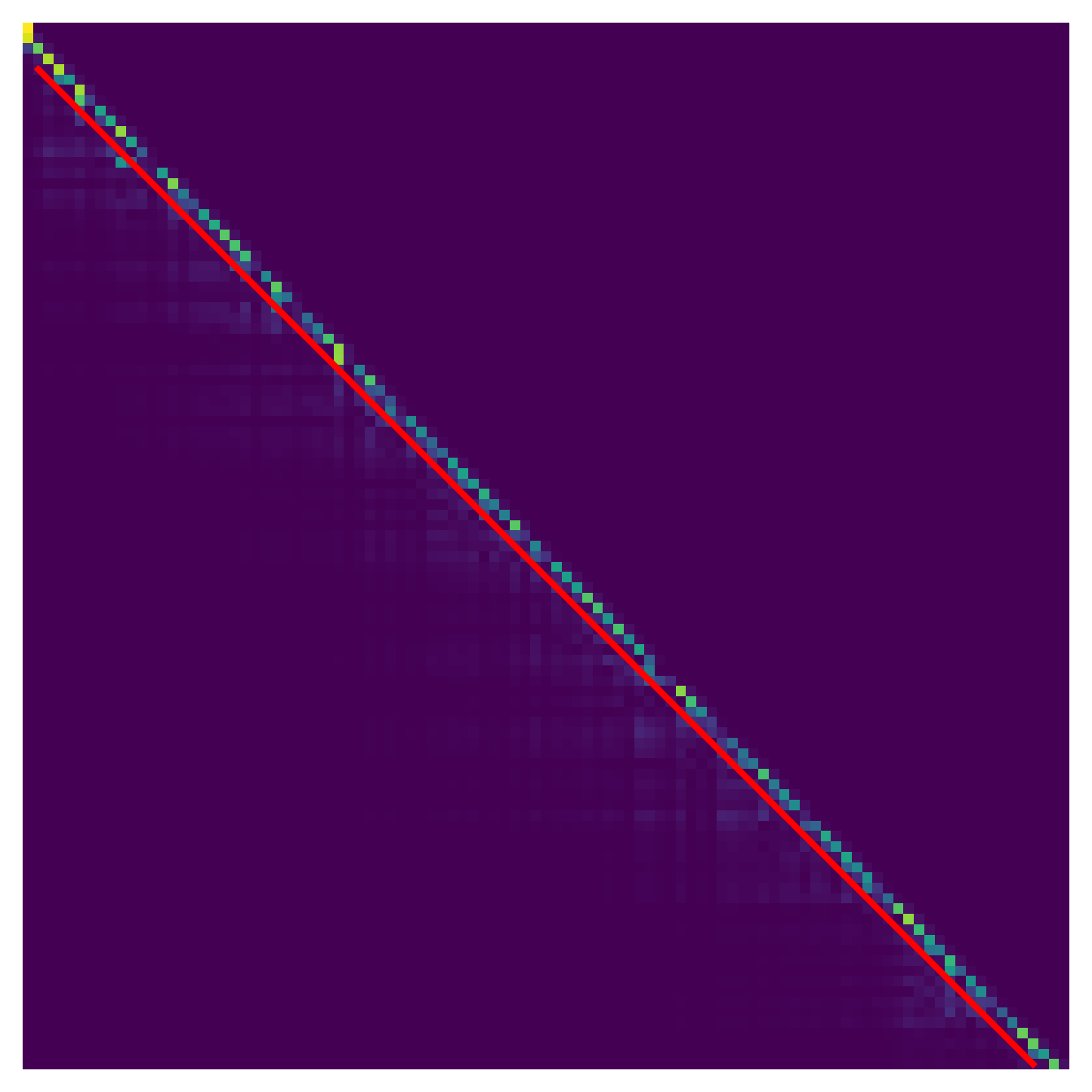
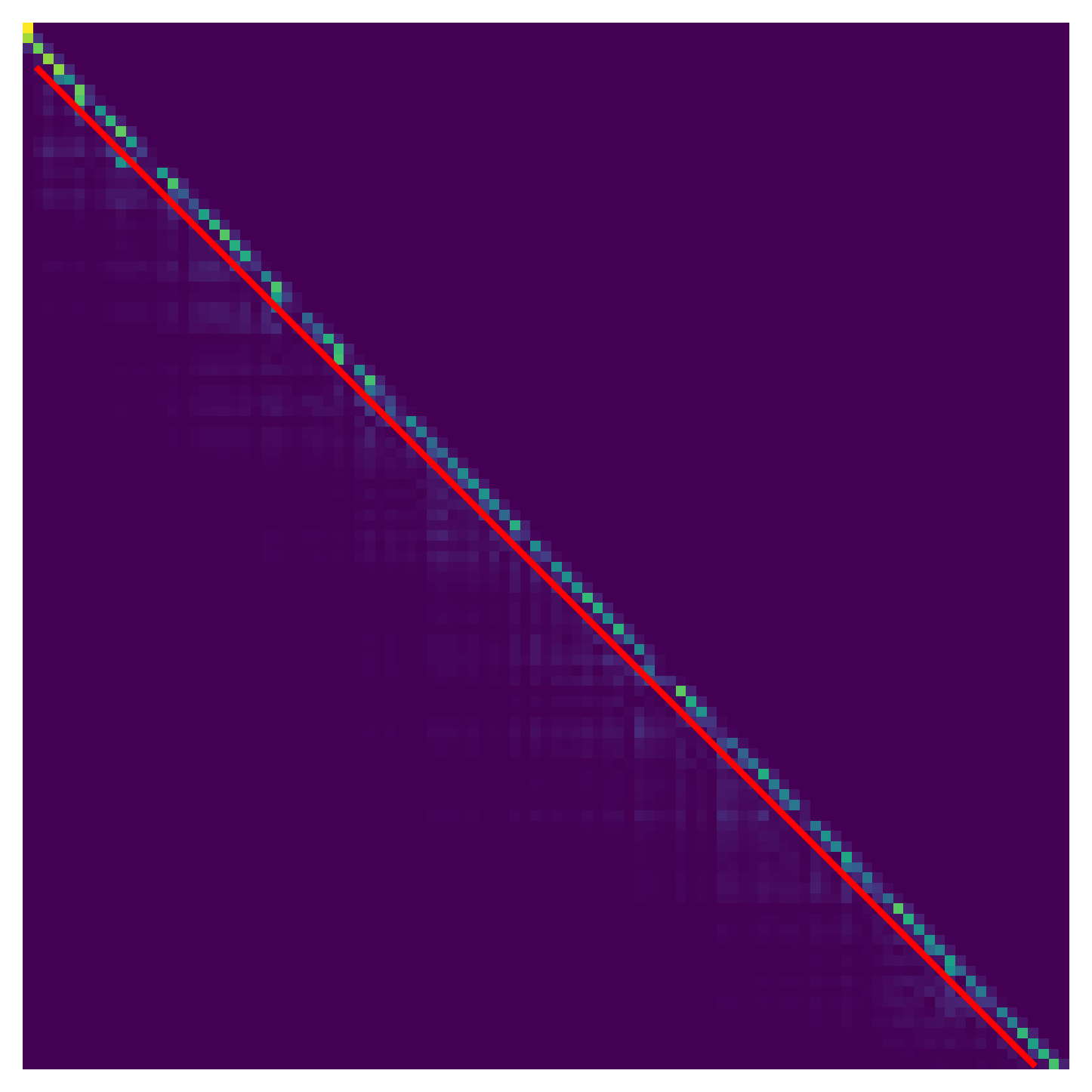
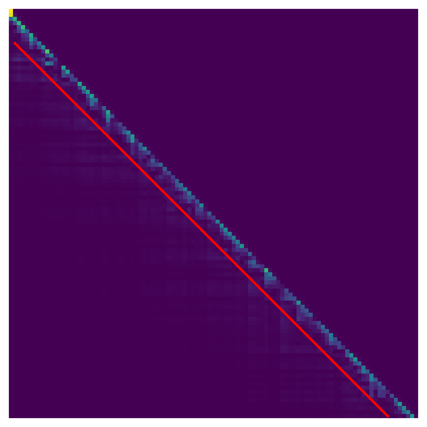
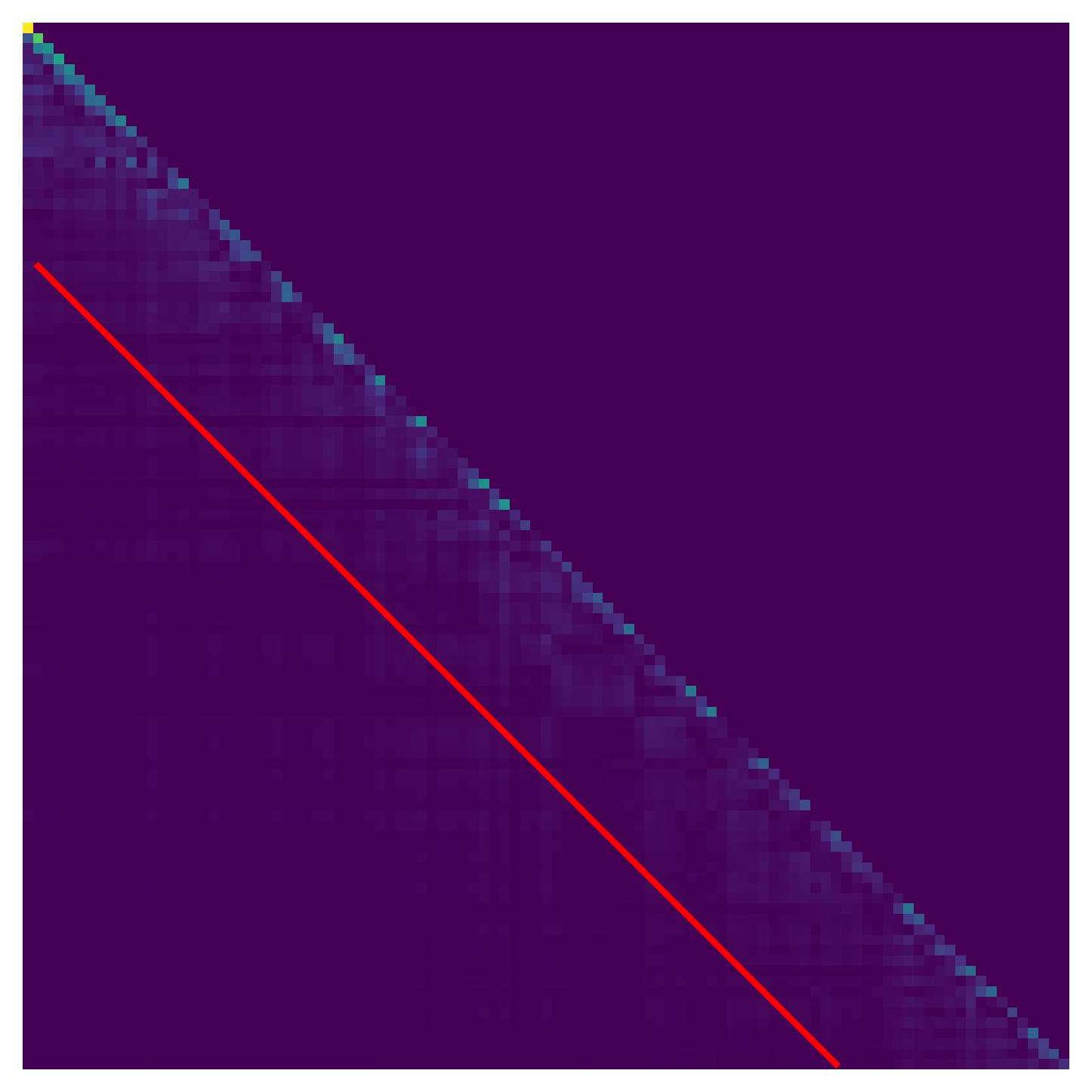
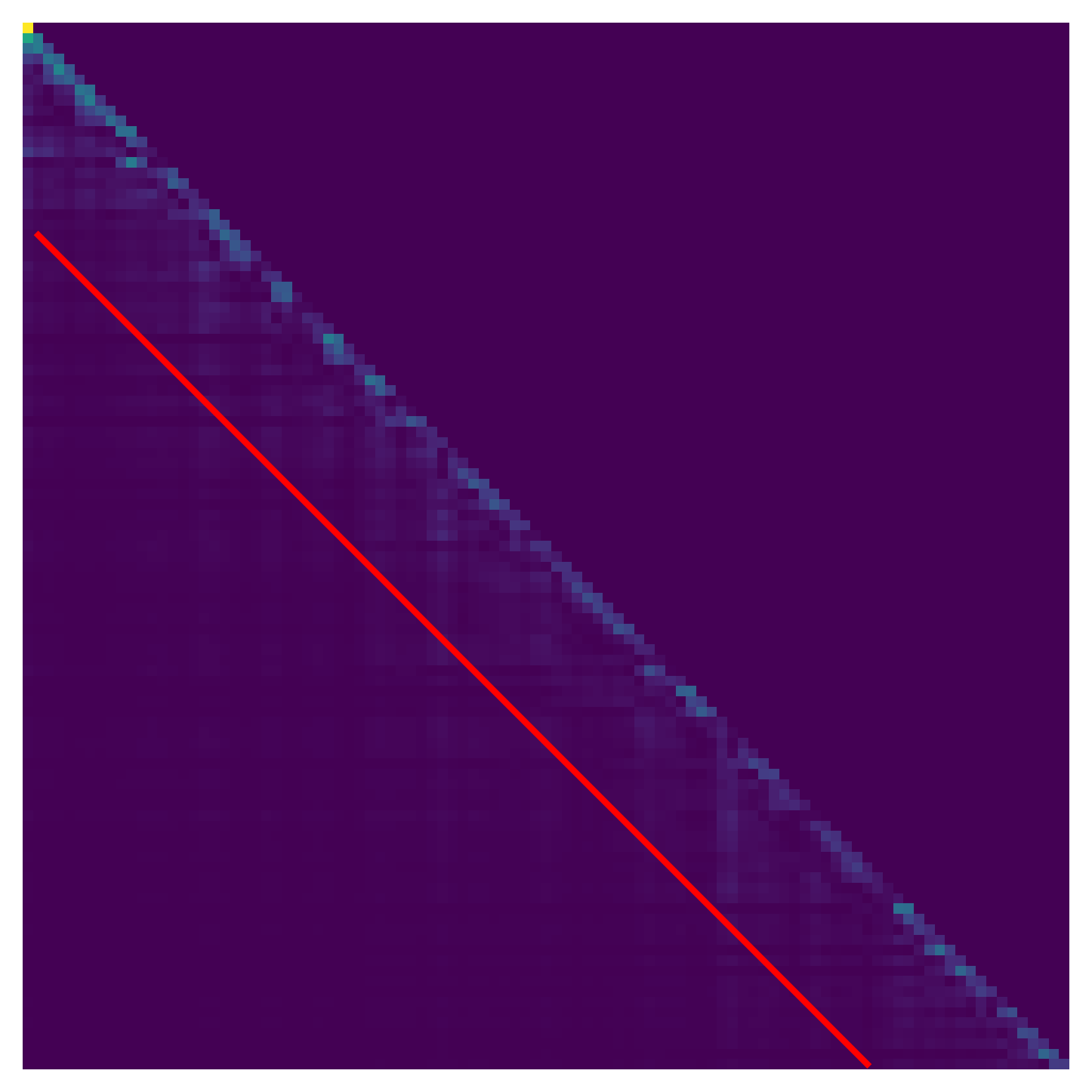
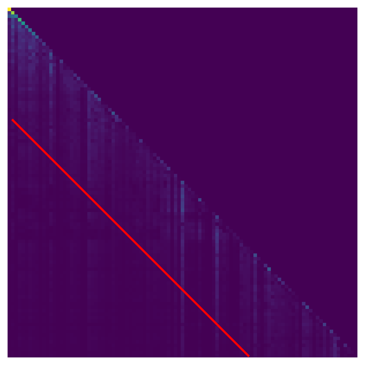
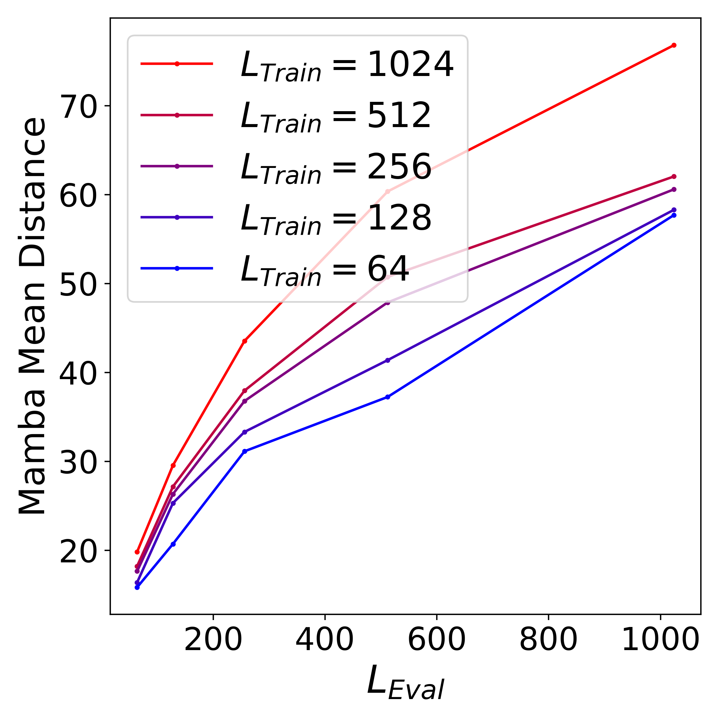
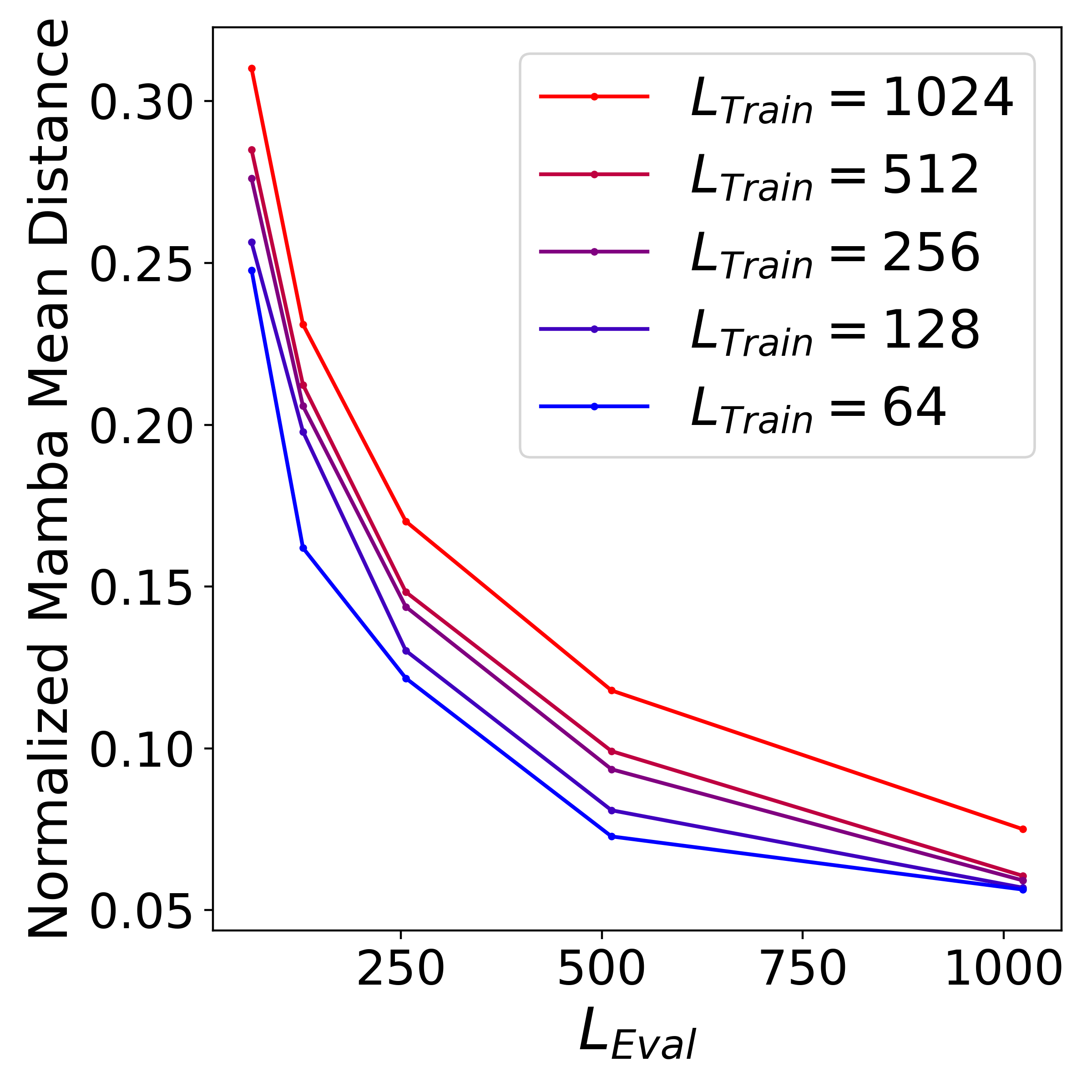
Figure 3: Mamba Mean Distance. Each panel contains an attention matrix along with its corresponding ’Mamba Mean Distance’, depicted by the distance of the red diagonal line from the main diagonal. The matrices are extracted from a pre-trained model of size 2.8B, trained on the Pile dataset Gao et al. (2020).

Figure 4: Mamba Mean Distance Quantifies Extrapolation Abilities. (Left) Mamba Mean Distance as a function of the context length during inference, for various training context lengths. (Right) Same, but normalized by the training context length.

By introducing an empirical measurement for Mamba’s ERF, we can explore it more robustly. Fig. 4 depicts how the Mamba Mean Distance is influenced when increasing the input sequence length during training and inference. Here, Mamba-based language models with 80M parameters are trained across various context lengths for next-token prediction on the WikiText-103 benchmark Merity et al. (2016). We average the Mamba Mean Distance over all channels and layers using 100 test examples.

The left panel of Fig. 4 shows that the Mamba Mean Distance increases with longer context lengths during both training and evaluation. However, this does not take into account the length of the context that needs attending to. In the right panel, we normalize the Mamba Mean Distance by the sequence length during inference, revealing that the proportion of context utilized in practice decreases as the context length during evaluation increases. This phenomenon suggests that the limited length-extrapolation capabilities of Mamba models are due to a reduced ERF (represented by the normalized Mamba Mean Distance), which diminishes as the context length increases during evaluation.

To better understand this phenomenon, we return to the implicit attention defined in Eq. 7. We note that the product of transition matrices $\prod_{k=j+1}^{i}\bar{A}_{k}$ includes more elements as the sequence length $L$ increases, and can be written for the last row as:

$$\vspace{-3pt}\prod_{k=j+1}^{L}\bar{A}_{k}=\prod_{k=j+1}^{L}\exp(A\Delta_{k})=\exp(A\sum_{k=j+1}^{L}\Delta_{k})$$ (11)

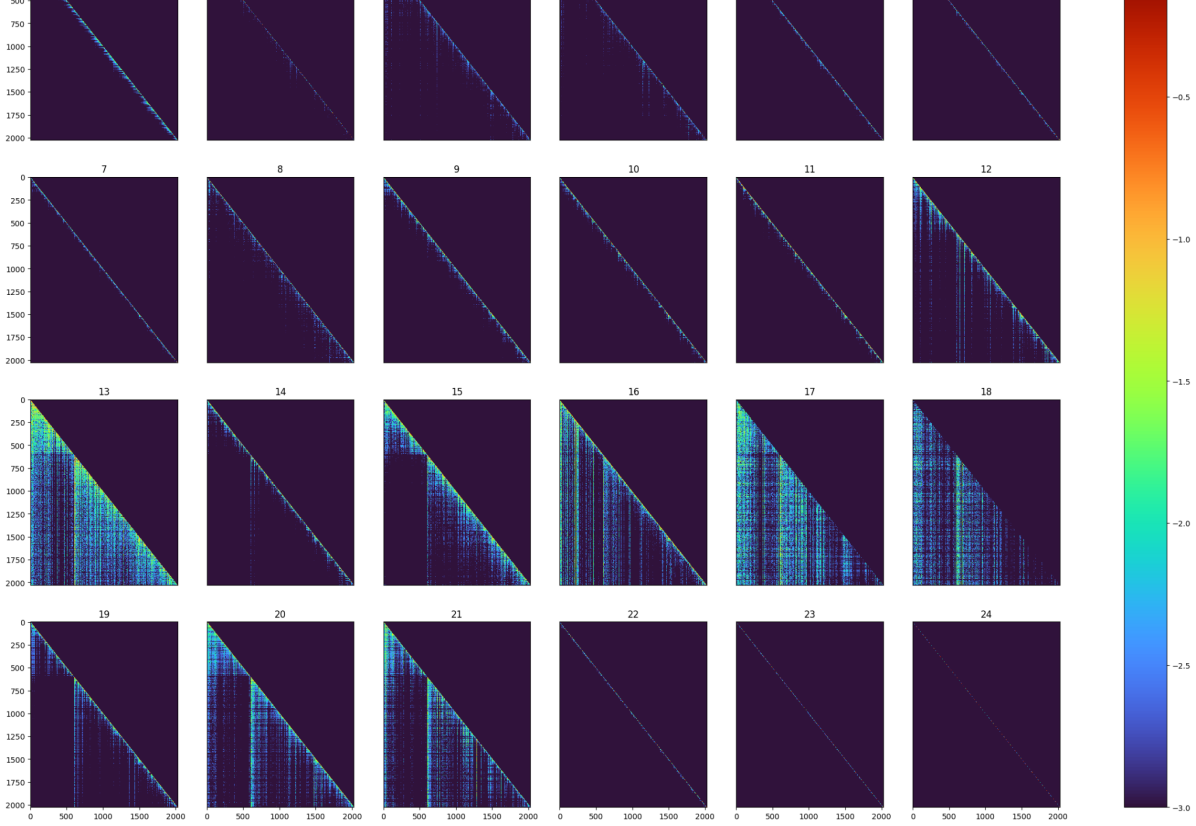
Figure 15: Normalized Mamba Attention Map. Displayed in log scale for each layer of the Mamba-130M model.

We note that this product always converges since $\Delta_{t}\geq 0$ and $A[i,i]<0$ by design. Yet, if it converges too fast, the attention element will collapse undesirably. To quantify the loss of information we focus on the attention element $\alpha_{L,1}$ due to the following reasons: (i) we are usually interested in the information at the end of the sequence; (ii) this element is the first in the row to collapse, capturing the first occasion of information loss because $\sum_{k=2}^{L}\Delta_{k}\geq\sum_{k=j+1}^{L}\Delta_{k}$ for all $L-1\geq j\geq 1$, and $A$ is always negative, so the power of its exponent will always be the smallest. We measure $\sum_{k=2}^{L}\Delta_{k}$ in Fig. 6 for varying evaluation context lengths L, per layer, averaged over the channels dimension. As can be seen in the figure, the values of $\sum_{k=2}^{L}\Delta_{k}$ increase exponentially fast in the most semantic layers (layers 16 and 17, see Passkey Retrieval in Sec. 5 for more details), leading to a fast collapse. Note that these are the layers where the worst ERFs are observed. The values of $\sum_{k=2}^{L}\Delta_{k}$ grow linearly in the other layers, which perform local processing (Fig. 15). Their decay is intentional.

A likely explanation for the limited length-generalization abilities is that during training, each SSM layer learns decay rates $A$ that are sufficient for processing training data of length $L_{train}$ but not flexible enough to provide effective length-extrapolation for lengths $L_{eval}>L_{train}$ . Specifically, if the decay rate is too high, long dependencies cannot be captured. Conversely, if the decay rate is too low, the state becomes “overloaded” with excessive information, which can obscure the important signals needed for effective processing.

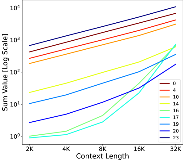
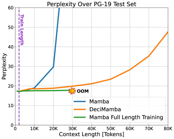
Figure 5: Quantifying Mamba’s Information Loss by Measuring $\sum_{k=2}^{L}\Delta_{k}$ Divergence. To show Mamba’s sensitivity to increasing context lengths we measure the first occasion of information loss, as described in Sec.3. We observe that in the most semantic layers (16 and 17, see Passkey Retrieval in Sec. 5) $\sum_{k=2}^{L}\Delta_{k}$ diverges exponentially fast, causing a fast decay in its respective attention value, leading to the ERF observed in Fig. 2.

Figure 6: Perplexity Over PG-19 Test Set. The dashed purple line shows the train sequence length for Mamba and DeciMamba (Mamba-130m). Each point on the green curve shows a different Mamba model trained on the respective context length ($L_{train}=L_{eval}$); for $L_{train}>30K$ an Out Of Memory (OOM) error occurs.

4 Method: DeciMamba

In Sec. 3 we identified that for a pre-trained model, the ERF of Mamba is dictated by the context size used during training $L_{train}$. This creates a blind spot for sequences that exceed $L_{train}$, as dependencies originating in the far input segments are not captured by the model, resulting in poor length generalization. To solve this problem we propose embedding a filtering mechanism within the pre-trained Mamba layers, with no need to re-train the model. The mechanism’s core task is to reduce the amount of tokens that the S6 layer processes, and it does so by discarding tokens of fewer importance. The entire method is visualized in Fig. 7 and encapsulates three aspects: (i) Decimation Strategy, (ii) Decimation Rate, and (iii) Decimation Scope.

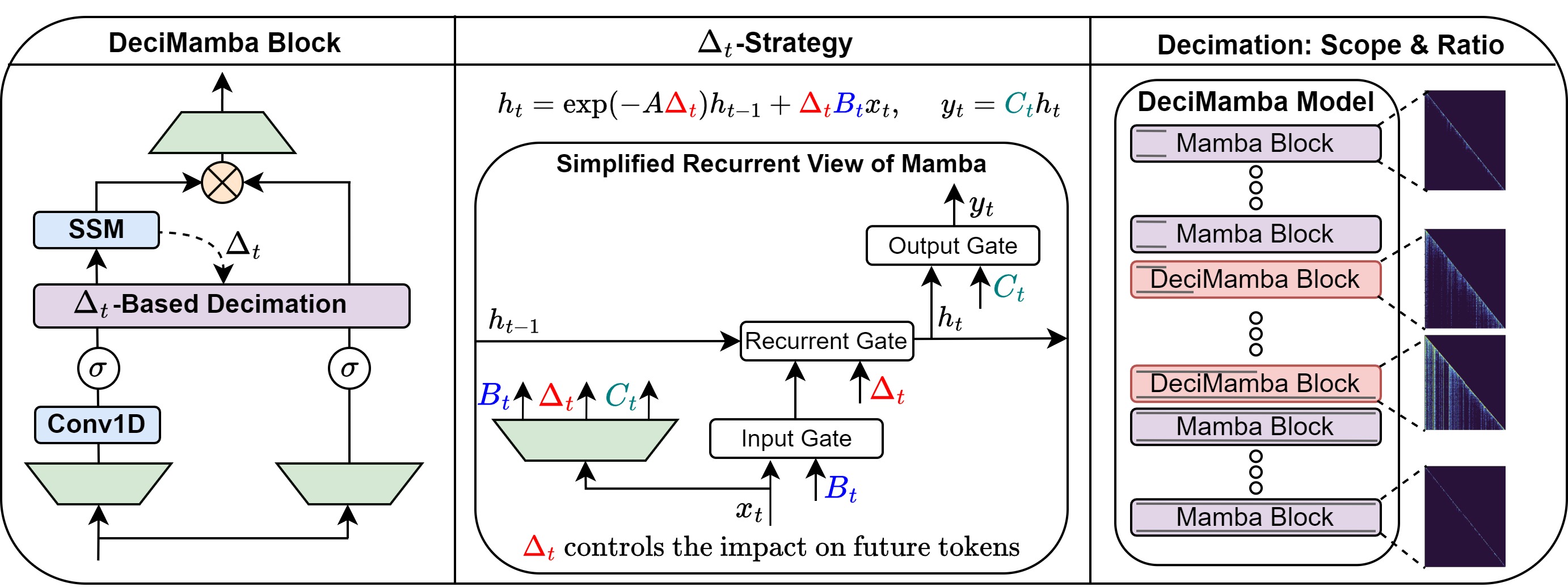
Figure 7: DeciMamba: (Left) Schematic overview of DeciMamba. (Middle) By carefully inspecting the recurrent view of Mamba, we revealed the implicit filtering mechanism embedded in the recurrent gate and controlled by $\Delta$. (Right) We visualize the DeciMamba model, illustrating the decimation ratio and scope. The grey lines represent the sequence length at the input and output of each layer, and layers with empirically long ERFs are decimated.

Decimation Strategy: The Role of $\Delta_{t}$  Unrolling Mamba’s recurrent rule (Eq. 12) reveals the link between the selective $\Delta_{t}$ and the token’s importance score for future tokens.

$$h_{t}=\bar{A}_{t}h_{t-1}+\bar{B}_{t}x_{t}=e^{A\Delta_{t}}h_{t-1}+\Delta_{t}B_{t}x_{t}.$$ (12)

When $\Delta_{t}\rightarrow 0$ the layer discards the input token and preserves the previous hidden state. When $\Delta_{t}>0$ the hidden state ’attends’ the input token (the attention is proportional to $\Delta_{t}$) and adds it to an attenuated version of the previous hidden state (this attenuation is also proportional to $\Delta_{t}$). We note that this is always the case because $\Delta_{t}\geq 0$ and $A[i,i]<0$ by design. Hence, $\Delta_{t}$ can be interpreted as the controller of the recurrent gate, determining which tokens should impact future tokens. Since Mamba ignores input tokens with small $\Delta_{t}$, it is natural to decimate them.

Decimation Ratio  For each decimating layer $s$, we propose to keep the Top-$P_{s}$ tokens with the largest mean $\Delta_{t}$ values (over the channels), where $P_{s}$ decreases gradually as we go deeper into the network according to the following formula:

$$P_{s}=L_{base}\cdot\beta^{s},\quad\beta\in(0,1),\quad L_{base}\in\mathbb{N}$$ (13)

where $\beta,L_{base}$ are hyper-parameters representing a decay factor that controls the decimation rate (as we progress in depth) and the maximal length of the sequence after the first decimating layer. Sec.5.1 further discusses the selected pooling strategy.

Decimation Scope: Layer Selection  We turn to describe the decimation scope, which defines which layers should use the embedded decimation mechanism. We begin by explaining the guiding principles behind our method, followed by the criteria that reflects those principles.

Our goal is to expand the ERF of a pre-trained Mamba model. Traditionally, DL models focus on various scales of token interactions at different layers. Therefore, a natural design choice is to decimate in layers that already focus on long-range dependencies. This approach can potentially increase their ability to learn global dependencies without negatively impacting the layers that are associated with short-term features.

As a criterion for measuring the scale embedded within each layer, we measure the ERF of Mamba based on the Mamba Mean Distance defined in Eq. 10. We thus select the layers with the highest Mamba Mean Distance, with the number of selected layers being a hyper-parameter.

5 Experiments

We evaluate DeciMamba as a context-extension approach across multiple tasks. Initially, we demonstrate the long-range understanding and retrieval capabilities of our method in the NLP domain. Subsequently, we assess the retrieval abilities of our method using the Passkey test, and examine the language modeling capabilities of DeciMamba.

Document Retrieval

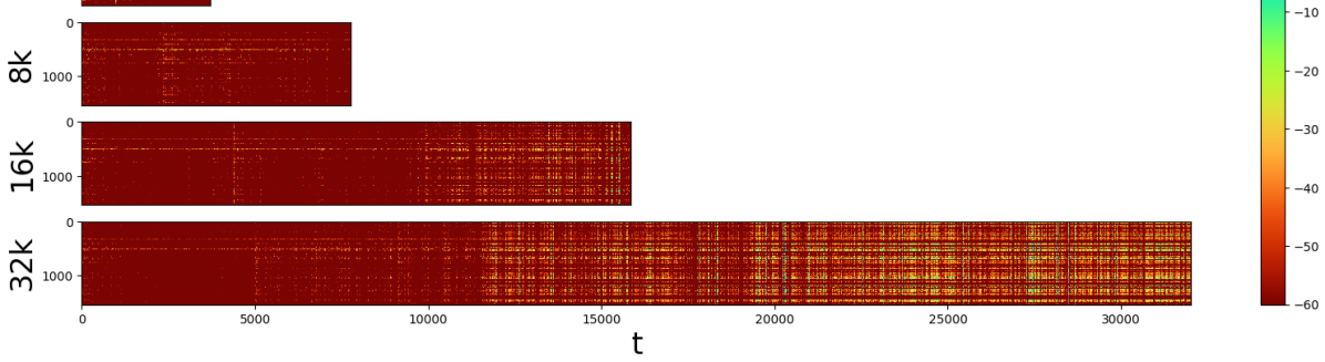
Figure 14: Measuring the Effects of Limited ERFs. We show the $\Delta_{t}$ values across the channels for layer 16 in the Mamba-130M model, examined on different context lengths. The horizontal and vertical axes indicate the token number and the channel respectively. As can be observed from the results above, the passkey can be detected clearly until the ERF ends (for $t>10K$).

We demonstrate DeciMamba’s extrapolation abilities in a real-world long-range NLP task. In this task the model receives a query and $N_{docs}$ randomly assorted documents, and its objective is to return the id of the document that holds the answer to the query. Our data is sampled from SQuAD v2 Rajpurkar et al. (2018). We train both Mamba-130m and DeciMamba-130m to retrieve out of $N_{docs}=11$ documents (about 2k tokens), and evaluate their performance with $N_{docs}\in[11,300]$ (2k tokens to 60,000 tokens). The results are presented in Fig. 1. While Mamba is able to retrieve until $N_{docs}=40$ documents, it suffers from a sharp decline when the amount of documents is further extended. For $N_{docs}=50$ the input sequence length is about 10k tokens, and as can be seen in Sec. 5 (Passkey Retrieval) and in Fig. 14, Mamba-130m starts to suffer from ERFs around this region when trained on 2k tokens. On the contrary, DeciMamba is able to extrapolate to sequences that are more than x25 times longer than the ones seen during training ($\sim 250$ documents), without any additional computational resources.

Multi-Document QA. Next, we stay in a setting similar to Sec. 5 (Document Retrieval), yet increase the level of difficulty by asking the model to answer the query in free text (instead of retrieving the id of the most relevant document). We train Mamba-130m and DeciMamba-130m on the same dataset and present the F1 score between the generated response and the ground truth answers in Tab. 1. As in the previous task, when the amount of documents is close to the amount trained on, the models perform quite similarly, with a slight advantage towards DeciMamba. When the document amount significantly increases we can see that DeciMamba develops a clear advantage. Yet, this time, due to the task’s difficulty, its performance decays as well. Note that Mamba’s and DeciMamba’s performance is relatively modest compared to prior work due to the use of smaller models, which limits the presented text generation capabilities.

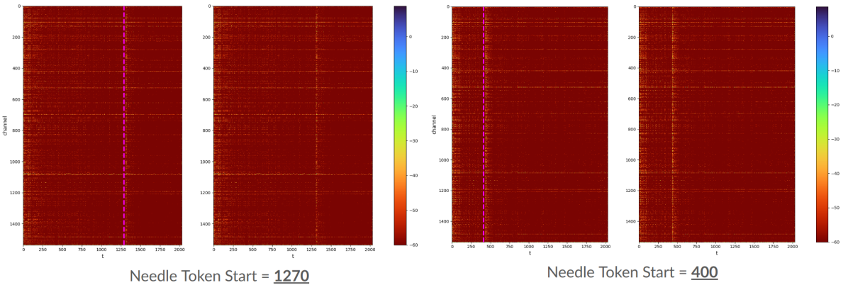
Figure 13: Demonstrating the ‘Importance-Scoring’ Abilities of $\Delta_{t}$. We evaluate Mamba-130M on the Passkey Retrieval task, and record the values of $\Delta_{t}$ for all channels of layer 16. Each pair of images is identical, except that the left one marks the location of the passkey with a dashed pink line. The horizontal and vertical axes indicate the token number and the channel respectively. As can be seen from the two cases examined above, the $\Delta_{t}$ activation captures the needle location successfully, demonstrating the effectiveness of its ‘importance scoring’ mechanism.

Passkey Retrieval. We fine-tune both Mamba-130M and DeciMamba-130M to retrieve a random 5-digit code hidden in a random location within a contiguous 2K token sample from Wiki-Text Merity et al. (2016). To test the models’ extrapolation abilities, during inference we increase the sequence lengths exponentially from 1K to 128K and record their performance for a variety of passkey locations within the context. Full implementation details can be found in Appendix A.1. As can be seen in Fig. 9, DeciMamba-130m significantly increases the extrapolation abilities of Mamba-130m from 16K to 128K, when trained on sequence lengths of 2k tokens only. Interestingly, we identify that the $\Delta_{t}$ values in Layer 16 of Mamba-130m capture the exact location of the passkey, as can be seen in Fig. 13. Using this finding, we display the distortion caused to the embedded sequence due to the ERF in Fig. 14. Tokens at locations < 10k have meaningful $\Delta_{t}$ values, yet tokens at locations > 10k have noisy $\Delta_{t}$’s, possibly due to the poor information flow caused by the ERF.

Language Modeling  Following Chen et al. (2023b); Mehta et al. (2022); Chen et al. (2023a), we evaluate our method on long-range language modeling using the PG-19 dataset in both zero-shot and fine-tuned regimes.

Zero-Shot. We test our method on the test set of PG-19 using the larger Mamba models (1.4b, 2.8b) in Fig. 9 (left). We observe that the selectivity scores learned during pre-training are quite effective and extend the context naturally without any training for both models. Furthermore, our method can maintain the low perplexity achieved in the short-context region. In the ablations section we further discuss our proposed decimation mechanism and show its benefit w.r.t other alternatives.

Fine-Tuning. We display DeciMamba’s performance on PG-19 perplexity in Fig. 6. We train both Mamba-130M and DeciMamba-130M with a sequence length of 2K and test their extrapolation abilities. The full training details can be found in Sec. A.4 in the appendix. While Mamba can extrapolate to context lengths that are at most x5 times longer than the training sequences, DeciMamba can extrapolate to sequences that are about x20 times longer, without any additional computational resources. Furthermore, we plot a lower bound by calculating the perplexity of a Mamba-130M model that was trained on the same context length it evaluates on (each point on the green curve is a different model). We observe that DeciMamba is close to the lower bound and diverges from it quite slowly, while utilizing significantly less computational resources. Nevertheless, for train sequences longer than 30K the ‘lower bound’ models reach an Out Of Memory (OOM) error (Nvidia RTX-A6000, 48GB of RAM), further emphasizing the importance of good extrapolation abilities when scaling to longer sequences.

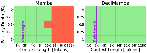
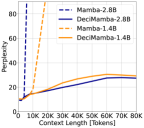
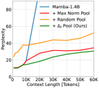
Figure 8: Passkey Retrieval. DeciMamba’s global pooling layer adapts the input sequence’s length to the effective receptive field learned during short-sequence training. This allows the model to extrapolate to sequences that are significantly longer. Results for Mamba-130m.

Figure 9: 0-shot perplexity over the PG-19 Test Set. (Left) Comparing Mamba with DeciMamba. (Right) An ablation studying the pooling mechanism, comparing ours (based on $\Delta_{t}$) to random or max-norm pooling.

#Docs	5	10	20	40	60	80	100	120	140	160
Mamba	23.5	25.3	22.8	23.6	25.8	19.3	7.5	4.1	1.1	0.6
+Deci	25.6	26.2	24.4	25.3	22.74	19.1	18.1	12.9	10.0	5.0

Table 1: Multi-Document QA. The table holds the F1 score between the ground truth annotations and the predictions of Mamba-130m and DeciMamba-130m (+Deci) across different number of documents. Both models were trained using 11 documents.

5.1 Ablations

Layer Selection  We ablate our layer selection methodology, as it has significant affect on the model’s performance (Figure 10). Each point on the curve represents the score achieved by a DeciMamba-130M model in the Passkey Retrieval task when trained on sequences of length 2K. The only difference between the models is the first decimating layer (x axis). We see that when the decimating layer is too shallow (e.g. layer 8), the model fails completely. As we increase the minimal decimating layer we observe a large increase in performance, until reaching the climax at layer 12. This result aligns with the fact that the $\Delta_{t}$ distribution is farther from 0 in Mamba’s early layers (all tokens are important). We hypothesize that the tokens still don’t have a strong representation at this stage, hence it makes less sense to decimate w.r.t their $\Delta_{t}$ value. After layer 12 the performance of DeciMamba starts to drop, and stabilizes at the vicinity of the baseline Mamba model. At this region we start decimating too late, as some long-dependency layers suffer from ERFs when processing the longer Passkey Retrieval sequences. The final layers (21-23) also have larger $\Delta_{t}$ values, so they should not be decimated as well. We hypothesize that these layers ’decode’ the processed embeddings back into token distributions, so the intermediate representations are yet again not fit for semantic decimation.

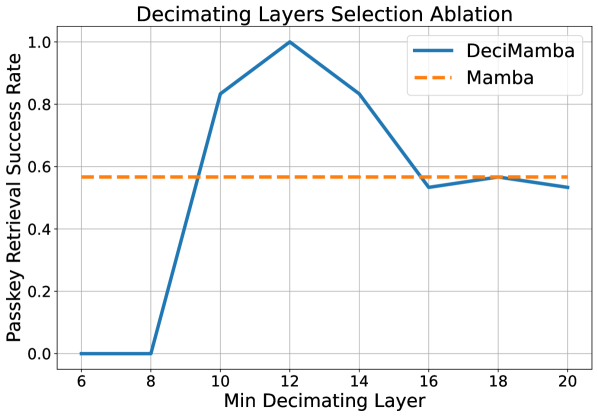
Figure 10: Layer Selection Ablation. Score achieved by DeciMamba-130M in the Passkey Retrieval task when trained on sequence lengths of 2K. All models differ by the first decimating layer (x axis) and stop decimating at layer 20. The result shows the model’s sensitivity to the selection of decimating layers.

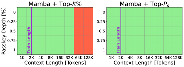
Figure 11: Pooling Strategy Ablation - Results. The figure compares two pooling strategies, Top-$P_{s}$ (ours) and Top-$K\%$. As shown, the Top-$K\%$ approach lags behind the Top-$P_{s}$ approach, demonstrating that our strategy allows the model to extrapolate to significantly longer sequences. Results are for Mamba-130m.

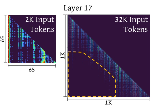
Figure 12: Pooling Strategy Ablation. Top-$K\%$ pooling leads to a limited ERF in layer 17. The size of the attention map is affected by the input sequence length: for $L_{eval}=2K$ layer 17 will process 65 tokens (left) and for $L_{eval}=32K$ it will process 1K tokens (right). Since $L_{train}=2K$, layer 17 has only seen training sequences of length 65, therefore suffers from an ERF when $L_{eval}$ increases (right, dashed orange shape).

Pooling Strategy  We show the importance of the proposed Top-$P_{s}$ pooling strategy in the following ablation study. Suppose we select a different pooling strategy, Top-$K\%$, which keeps the top $K\%$ tokens with the largest mean $\Delta_{t}$ values (over the channels dimension). We train a DeciMamba-130m model for the Passkey Retrieval task on sequences of length $L_{train}=2K$, with $K=50\%$ and decimation layers [12,…,20]. As can be seen in Fig. 11 (Appendix), Top-$K\%$ extends Mamba’s extrapolation abilities from 8K to 32K, yet does not do as well as Top-$P_{s}$ which extends to 128K. While Top-$K\%$ decimation decreases the sequence length greatly (the output is x512 times shorter), during extrapolation each SSM layer still faces input sequences that are much longer than the ones it has seen during training, as demonstrated in Fig. 12. We further explain this result; During training Layer 17 saw sequences of length 65 ($L_{train}=2K$, followed by a decimation rate of 50% in each layer from layer 12). During inference it sees sequences of lengths 65 and 1002 (where $L_{eval}=2K,32K$, left and right images, respectively). Since the sequence length at layer 17 of the latter (1K) is much longer than the one it saw during training (65), the extrapolation is limited by an ERF (right image, dashed orange shape). This shows the importance of keeping the lengths of the inputs to each decimating SSM layer similar to the ones seen during training, as done by Top-$P_{s}$.

Decimation Mechanism.  To emphasize the benefit of pooling w.r.t the values of $\Delta_{t}$, we examine two additional decimation mechanisms: max-norm decimation (tokens with maximal norm are kept) and random decimation (tokens are randomly kept). We equip Mamba-1.4b with each of the decimation mechanisms (decimation layer = 12, $L_{base}=8000$), and compare each model’s zero-shot perplexity in Fig. 9 (right). Max-norm pooling achieves a similar trend to $\Delta_{t}$ pooling (DeciMamba), yet performs somewhat worse. The result suggests that $\Delta_{t}$ is a better candidate for pooling, but also shows that the token’s norm also holds some information about its importance. We hypothesize that a method that combines both might achieve better performance than any one alone, but leave this question open for future work. Random pooling induces strong distortion to the embedded sequence, yet achieves better perplexity for longer contexts. This surprising result demonstrates how sensitive Mamba is to ERFs - in longer sequences, it is actually better to randomly decimate the sequence rather than process its full length.

6 Conclusions

In this paper, we explore the length-extrapolation abilities of S6 layers. Our first contribution is the characterization of the ERF of S6. This characterization reveals that the ERF of Mamba is significantly constrained by the context length during training, which is counterintuitive given that Mamba theoretically has an unbounded receptive field due to its recurrent selective memory. Based on these insights, we develop DeciMamba, a unique data-dependent compression operator that is built on two key insights: (i) There exists a hidden filtering mechanism within the Mamba layer, manifested by the selective time-steps $\Delta_{t}$, which can be interpreted as the controller of the recurrent gate. (ii) Long-range and short-range interactions between tokens are captured by different layers in the model, which can be identified using our Mamba Mean Distance metric.

Looking ahead, we plan to explore different transformer context-extension methods, including length-extrapolation PE Press et al. (2021); Golovneva et al. (2024), hierarchical models, and architectural improvements Sun et al. (2022). Furthermore, we intend to extend our analysis to other layers beyond S6, e.g., RWKV, xLSTM, and more.

7 Limitations

Our model modifies a pretrained Mamba model but does not propose an improved Mamba architecture to address the underlying issue. Despite empirical evidence demonstrating the effectiveness of our decimation-based method in capturing long-range interactions and its efficiency, the approach can be suboptimal. For example, pooling and compression methods may miss critical information in challenging scenarios. Therefore, designing an improved Mamba variant with enhanced length-generalization abilities that can effectively capture global interactions within a single layer (without pooling the sequence) is an important next step.

8 Ethics Statement

This work analyzes and improves the performance of large language models (LLMs) for long context understanding, which is crucial when deploying them in real-world systems. This improvement is anticipated to have a positive impact on the use of LLMs in society. However, we acknowledge that LLMs could propagate biases. We emphasize the necessity of further research into these biases before our work can be applied reliably beyond the research environment.

Appendix A Experimental Details

All model checkpoints are taken from the Hugging Face Model Hub:

• state-spaces/mamba-130m

• state-spaces/mamba-370m

• state-spaces/mamba-790m

• state-spaces/mamba-1.4b

• state-spaces/mamba-2.8b

Our code is based on the official Mamba implementation.

A.1 Passkey Retrieval

Each model is trained for 5 epochs with a learning rate of 1e-4, gradient clipping of 1, batch size of 32 (used batch accumulation) and AdamW optimizer Kingma and Ba (2017) with weight decay of 0.1. In each epoch the models train over 6144 sequences of length 2K. For DeciMamba-130M we use $L\_base=2K$, $\beta=0.5$, $decimating\_layers=[13,...,21],min\_seq\_len=20$.

A.2 Document Retrieval

We train each model with data from SQuAD v2 Rajpurkar et al. (2018), which provides examples in the form of (Query, Document, Answer). Our training samples have the following form: <$Query$>; $N_{docs}\times$<$Document$>; <$Answer$>, where <$Document$> can be either the golden document (which holds the answer to the query) or one of $N_{docs}-1$ randomly sampled documents. <$Answer$> holds the id of the golden document. In our setting $N_{docs}=11$, the order of the documents is random, and the query and respective document id are appended to the beginning of each document. During Evaluation we use the same setting but vary the value of $N_{docs}$, between 11 and 300. We note that an average document in SQuAD has a length of about 200 tokens, so our average training sample has about 2,000 tokens, and the evaluation samples vary between 2,000 tokens to 60,000 tokens. We train for one epoch with 300 steps, use a learning rate of 1e-4, gradient clipping of 1, batch size of 64 (used batch accumulation) and AdamW optimizer with weight decay of 0.1.

A.3 Multi-Document Question Answering With Free Text Response

We operate in a similar setting as in Section A.2, but instead of predicting the tokens of the id of the relevant document we let the model generate a free-text response and measure it’s F1 score w.r.t a set of ground truth answers. We train each model for one epoch on the full SQuAD train set (about 90,000 examples when leaving out the samples intended for negative sampling, which do not have a ground-truth answer). We found that the optimal decimation parameters are decimation_layer = 14, $L_{base}$=2000 during training and $L_{base}$=7000 during evaluation. We intentionally decreased Lbase during training so the model could experience decimation during the training period ($L_{train}$ was a bit higher than $L_{base}$), because otherwise the training of DeciMamba and Mamba would have been identical. We use a learning rate of 1e-4, gradient clipping of 1, batch size of 64 (used batch accumulation) and AdamW optimizer with weight decay of 0.1.

A.4 PG-19 Perplexity

We train each model on a total of 100M tokens with a learning rate of 1e-4, gradient clipping of 1, batch size of 250 (used batch accumulation) and AdamW optimizer with weight decay of 0.1. During training we sample a single window from each example and train on it (For the extrapolating models the window length is 2K, for the lower bound models the window length is equal to the context length trained on). During evaluation, for each example we evaluate 10 windows with a maximal constant stride. We evaluate only the last 100 labels in each window, which represent the extrapolation abilities of the model at sequence lengths in the range of [$ctx\_len-100,ctx\_len$], providing an approximation to the model’s performance at the wanted $ctx\_len$. For DeciMamba-130M we use $L\_base=2K$, $\beta=0.83$, $decimating\_layers=[12,...,20],min\_seq\_len=20$. During evaluation we keep the same parameters except setting $L\_base=8K$. Additionally, in this specific task DeciMamba was trained with a similar, yet not identical, Language Modeling (LM) loss. We break the labels sequence (length = 2K) into two chunks. The first 1K labels are trained conditionally on the first 1K tokens of the sequence (like vanilla LM). The last 1K labels are trained conditionally on the whole sequence (2K), and DeciMamba was configured to compress the first 1K input tokens. This way we are able to train DeciMamba to compress context while training on each label in the sequence, making the training much more efficient. We also experimented with chunking the labels into more than two chunks, but only experienced a slowdown in computation while achieving similar performance. For the lower bound models we had to reduce the amount of training steps in order to constrain the training to 100M tokens. Specifically, for each context length, we followed the following formula: $num\_of\_steps=100M/(batch\_size*ctx\_len)=100M/(250*ctx\_len)$. For the Zero-Shot perplexity test for the 1.4b model we used Layer 12 for decimation and $L_{base}=4000$. For the 2.8b model we used Layer 22 for decimation and $L_{base}=4000$.

Appendix B Other Related Work

B.1 Long Range Transformers.

Transformers have emerged as highly effective models for various tasks, yet their widespread adoption has been constrained by their limited long-range modeling capabilities. Thus, applying transformers effectively to long-range data remains a central challenge in DL, particularly in NLP. A primary factor in this challenge is that the effective context of transformers is dominated by the context observed during training, which is limited because training LLMs on datasets with billions of tokens across lengthy sequences is computationally demanding. Hence, three main approaches have been developed to tackle this problem: (i) creating efficient variants of transformers that allow an increase in the length of sequences during training. (ii) Context extension methods, which enable training on short sequences and evaluation on long sequences, and finally, (iii) hierarchical models that rely on pooling, chunking, and compression. Despite these extensive efforts, several recent studies indicate that high-quality handling of long text remains an unresolved issue Liu et al. (2024a); Li et al. (2024).

Efficient transformers. Over the years, many approaches have been proposed for making transformers more efficient Tay et al. (2022); Fournier et al. (2023). The two most prominent directions are hardware-aware implementations such as flash-attention Dao et al. (2022); Dao (2023) and ring-attention Liu et al. (2023), which accelerate computations over long sequences by several orders of magnitude. Additionally, developing efficient attention variants with sub-quadratic complexity has become very popular. Two notable examples are Linformer Wang et al. (2020), which utilizes a low-rank attention matrix, and Performer Choromanski et al. (2020), a variant that approximates the attention operator through a kernel function.

References

- Ali et al. (2024) Ameen Ali, Itamar Zimerman, and Lior Wolf. 2024. The hidden attention of mamba models. Preprint, arXiv:2403.01590.
- Beck et al. (2024) Maximilian Beck, Korbinian Pöppel, Markus Spanring, Andreas Auer, Oleksandra Prudnikova, Michael Kopp, Günter Klambauer, Johannes Brandstetter, and Sepp Hochreiter. 2024. xlstm: Extended long short-term memory. arXiv preprint arXiv:2405.04517.
- Chen et al. (2023a) Shouyuan Chen, Sherman Wong, Liangjian Chen, and Yuandong Tian. 2023a. Extending context window of large language models via positional interpolation. arXiv preprint arXiv:2306.15595.
- Chen et al. (2023b) Yukang Chen, Shengju Qian, Haotian Tang, Xin Lai, Zhijian Liu, Song Han, and Jiaya Jia. 2023b. Longlora: Efficient fine-tuning of long-context large language models. arXiv preprint arXiv:2309.12307.
- Choromanski et al. (2020) Krzysztof Choromanski, Valerii Likhosherstov, David Dohan, Xingyou Song, Andreea Gane, Tamas Sarlos, Peter Hawkins, Jared Davis, Afroz Mohiuddin, Lukasz Kaiser, et al. 2020. Rethinking attention with performers. arXiv preprint arXiv:2009.14794.
- Dao (2023) Tri Dao. 2023. Flashattention-2: Faster attention with better parallelism and work partitioning. arXiv preprint arXiv:2307.08691.
- Dao et al. (2022) Tri Dao, Dan Fu, Stefano Ermon, Atri Rudra, and Christopher Ré. 2022. Flashattention: Fast and memory-efficient exact attention with io-awareness. Advances in Neural Information Processing Systems, 35:16344–16359.
- De et al. (2024) Soham De, Samuel L Smith, Anushan Fernando, Aleksandar Botev, George Cristian-Muraru, Albert Gu, Ruba Haroun, Leonard Berrada, Yutian Chen, Srivatsan Srinivasan, et al. 2024. Griffin: Mixing gated linear recurrences with local attention for efficient language models. arXiv preprint arXiv:2402.19427.
- Dosovitskiy et al. (2020) Alexey Dosovitskiy, Lucas Beyer, Alexander Kolesnikov, Dirk Weissenborn, Xiaohua Zhai, Thomas Unterthiner, Mostafa Dehghani, Matthias Minderer, Georg Heigold, Sylvain Gelly, et al. 2020. An image is worth 16x16 words: Transformers for image recognition at scale. arXiv preprint arXiv:2010.11929.
- Fournier et al. (2023) Quentin Fournier, Gaétan Marceau Caron, and Daniel Aloise. 2023. A practical survey on faster and lighter transformers. ACM Computing Surveys, 55(14s):1–40.
- Gao et al. (2020) Leo Gao, Stella Biderman, Sid Black, Laurence Golding, Travis Hoppe, Charles Foster, Jason Phang, Horace He, Anish Thite, Noa Nabeshima, et al. 2020. The pile: An 800gb dataset of diverse text for language modeling. arXiv preprint arXiv:2101.00027.
- Golovneva et al. (2024) Olga Golovneva, Tianlu Wang, Jason Weston, and Sainbayar Sukhbaatar. 2024. Contextual position encoding: Learning to count what’s important. arXiv preprint arXiv:2405.18719.
- Gu and Dao (2023) Albert Gu and Tri Dao. 2023. Mamba: Linear-time sequence modeling with selective state spaces. arXiv preprint arXiv:2312.00752.
- Gu et al. (2021a) Albert Gu, Karan Goel, and Christopher Ré. 2021a. Efficiently modeling long sequences with structured state spaces. arXiv preprint arXiv:2111.00396.
- Gu et al. (2021b) Albert Gu, Isys Johnson, Karan Goel, Khaled Saab, Tri Dao, Atri Rudra, and Christopher Ré. 2021b. Combining recurrent, convolutional, and continuous-time models with linear state space layers. Advances in neural information processing systems, 34:572–585.
- Gupta et al. (2022) Ankit Gupta, Albert Gu, and Jonathan Berant. 2022. Diagonal state spaces are as effective as structured state spaces. Advances in Neural Information Processing Systems, 35:22982–22994.
- Kazemnejad et al. (2024) Amirhossein Kazemnejad, Inkit Padhi, Karthikeyan Natesan Ramamurthy, Payel Das, and Siva Reddy. 2024. The impact of positional encoding on length generalization in transformers. Advances in Neural Information Processing Systems, 36.
- Kingma and Ba (2017) Diederik P. Kingma and Jimmy Ba. 2017. Adam: A method for stochastic optimization. Preprint, arXiv:1412.6980.
- Li et al. (2024) Tianle Li, Ge Zhang, Quy Duc Do, Xiang Yue, and Wenhu Chen. 2024. Long-context llms struggle with long in-context learning. arXiv preprint arXiv:2404.02060.
- Liu et al. (2023) Hao Liu, Matei Zaharia, and Pieter Abbeel. 2023. Ring attention with blockwise transformers for near-infinite context. arXiv preprint arXiv:2310.01889.
- Liu et al. (2024a) Nelson F Liu, Kevin Lin, John Hewitt, Ashwin Paranjape, Michele Bevilacqua, Fabio Petroni, and Percy Liang. 2024a. Lost in the middle: How language models use long contexts. Transactions of the Association for Computational Linguistics, 12:157–173.
- Liu et al. (2024b) Yue Liu, Yunjie Tian, Yuzhong Zhao, Hongtian Yu, Lingxi Xie, Yaowei Wang, Qixiang Ye, and Yunfan Liu. 2024b. Vmamba: Visual state space model. arXiv preprint arXiv:2401.10166.
- Mehta et al. (2022) Harsh Mehta, Ankit Gupta, Ashok Cutkosky, and Behnam Neyshabur. 2022. Long range language modeling via gated state spaces. arXiv preprint arXiv:2206.13947.
- Merity et al. (2016) Stephen Merity, Caiming Xiong, James Bradbury, and Richard Socher. 2016. Pointer sentinel mixture models. Preprint, arXiv:1609.07843.
- Mohtashami and Jaggi (2023) Amirkeivan Mohtashami and Martin Jaggi. 2023. Landmark attention: Random-access infinite context length for transformers. arXiv preprint arXiv:2305.16300.
- Peng et al. (2023a) Bo Peng, Eric Alcaide, Quentin Anthony, Alon Albalak, Samuel Arcadinho, Stella Biderman, Huanqi Cao, Xin Cheng, Michael Chung, Matteo Grella, et al. 2023a. Rwkv: Reinventing rnns for the transformer era. arXiv preprint arXiv:2305.13048.
- Peng et al. (2023b) Bowen Peng, Jeffrey Quesnelle, Honglu Fan, and Enrico Shippole. 2023b. Yarn: Efficient context window extension of large language models. arXiv preprint arXiv:2309.00071.
- Pióro et al. (2024) Maciej Pióro, Kamil Ciebiera, Krystian Król, Jan Ludziejewski, and Sebastian Jaszczur. 2024. Moe-mamba: Efficient selective state space models with mixture of experts. arXiv preprint arXiv:2401.04081.
- Poli et al. (2023) Michael Poli, Stefano Massaroli, Eric Nguyen, Daniel Y Fu, Tri Dao, Stephen Baccus, Yoshua Bengio, Stefano Ermon, and Christopher Ré. 2023. Hyena hierarchy: Towards larger convolutional language models. In International Conference on Machine Learning, pages 28043–28078. PMLR.
- Press et al. (2021) Ofir Press, Noah A Smith, and Mike Lewis. 2021. Train short, test long: Attention with linear biases enables input length extrapolation. arXiv preprint arXiv:2108.12409.
- Raffel et al. (2020) Colin Raffel, Noam Shazeer, Adam Roberts, Katherine Lee, Sharan Narang, Michael Matena, Yanqi Zhou, Wei Li, and Peter J Liu. 2020. Exploring the limits of transfer learning with a unified text-to-text transformer. Journal of machine learning research, 21(140):1–67.
- Rajpurkar et al. (2018) Pranav Rajpurkar, Robin Jia, and Percy Liang. 2018. Know what you don’t know: Unanswerable questions for squad. Preprint, arXiv:1806.03822.
- Schiff et al. (2024) Yair Schiff, Chia-Hsiang Kao, Aaron Gokaslan, Tri Dao, Albert Gu, and Volodymyr Kuleshov. 2024. Caduceus: Bi-directional equivariant long-range dna sequence modeling. arXiv preprint arXiv:2403.03234.
- Shams et al. (2024) Siavash Shams, Sukru Samet Dindar, Xilin Jiang, and Nima Mesgarani. 2024. Ssamba: Self-supervised audio representation learning with mamba state space model. arXiv preprint arXiv:2405.11831.
- Su et al. (2024) Jianlin Su, Murtadha Ahmed, Yu Lu, Shengfeng Pan, Wen Bo, and Yunfeng Liu. 2024. Roformer: Enhanced transformer with rotary position embedding. Neurocomputing, 568:127063.
- Sun et al. (2022) Yutao Sun, Li Dong, Barun Patra, Shuming Ma, Shaohan Huang, Alon Benhaim, Vishrav Chaudhary, Xia Song, and Furu Wei. 2022. A length-extrapolatable transformer. arXiv preprint arXiv:2212.10554.
- Tay et al. (2022) Yi Tay, Mostafa Dehghani, Dara Bahri, and Donald Metzler. 2022. Efficient transformers: A survey. ACM Computing Surveys, 55(6):1–28.
- Vaswani et al. (2017) Ashish Vaswani, Noam Shazeer, Niki Parmar, Jakob Uszkoreit, Llion Jones, Aidan N Gomez, Łukasz Kaiser, and Illia Polosukhin. 2017. Attention is all you need. Advances in neural information processing systems, 30.
- Wang et al. (2024) Junxiong Wang, Tushaar Gangavarapu, Jing Nathan Yan, and Alexander M Rush. 2024. Mambabyte: Token-free selective state space model. arXiv preprint arXiv:2401.13660.
- Wang et al. (2020) Sinong Wang, Belinda Z Li, Madian Khabsa, Han Fang, and Hao Ma. 2020. Linformer: Self-attention with linear complexity. arXiv preprint arXiv:2006.04768.
- Zhu et al. (2024) Lianghui Zhu, Bencheng Liao, Qian Zhang, Xinlong Wang, Wenyu Liu, and Xinggang Wang. 2024. Vision mamba: Efficient visual representation learning with bidirectional state space model. arXiv preprint arXiv:2401.09417.