Ambiguity Clustering: an accurate and efficient decoder for qLDPC codes

Error correction allows a quantum computer to preserve a state long beyond the decoherence time of its physical qubits by encoding logical qubits in a larger number of physical qubits. The leading proposal for a scheme of quantum error correction is based on the surface code, but several recently proposed quantum low-density parity check (qLDPC) codes allow more logical information to be encoded in significantly fewer physical qubits. Key to any scheme of quantum error correction is the decoder, an algorithm that estimates the error state of the qubits from the results of syndrome measurements performed on them. The surface code has a variety of fast and accurate decoders, but the state-of-the-art decoder for general qLDPC codes, BP-OSD, has a high computational complexity. Here we introduce Ambiguity Clustering (AC), an algorithm which seeks to divide the measurement data into clusters which are decoded independently. We benchmark AC on the recently proposed bivariate bicycle codes and find that, at physically realistic error rates, AC is between one and three orders of magnitude faster than BP-OSD with no reduction in logical fidelity. Our CPU implementation of AC is already fast enough to decode the 144-qubit Gross code in real time for neutral atom and trapped ion systems.

Quantum computing has the potential to enable breakthrough calculations in high impact fields including pharmaceutical [1] and material [2] simulation and cryptography [3]. Practical advantage in these areas, however, will only come with fault-tolerant quantum computing, where the constituent qubits of the computer are encoded with sufficient redundancy to endure the rapid and inevitable errors to which they are subject. Such a fault-tolerant system requires an encoding scheme—a quantum code—for the qubits, in which the state of some number of logical qubits is encoded in a larger number of physical qubits. The scheme also prescribes sets of measurements to be performed on the physical qubits, from which one can estimate whether an error has occurred and, if it has, determine an appropriate correction. This calculation is referred to as decoding. Here we describe Ambiguity Clustering, a new decoding algorithm applicable to arbitrary quantum low-density parity check (qLDPC) codes.

A quantum code is qLDPC if each prescribed measurement involves only a small number of physical qubits, and each physical qubit is involved in only a small number of measurements. These are natural conditions for any practical scheme of fault-tolerant computation. The most widely studied quantum code is Kitaev’s surface code [4]. In addition to being qLDPC, the pattern of measurement allows surface codes to be implemented on a flat surface using a square grid of qubits and nearest-neighbour interactions. This is a useful property for systems such as superconducting circuits where qubits are implemented as immovable circuit elements. The surface code also has excellent decoders. It was remarked in Kitaev’s original paper that decoding can be reduced to the problem of finding minimum-weight perfect matchings in a graph. This can be solved exactly in polynomial time by Edmonds’ Blossom algorithm [5], and more recently approximated in almost-linear time by the Union-Find decoder [6].

The surface code has a high overhead: a great number of physical qubits are required to encode a single logical qubit. Recently much work has focused on the development of more general qLDPC codes [7, 8, 9, 10]. These have the potential to encode many more logical qubits in a given set of physical qubits, whilst maintaining a similar level of protection. In return, we must [11] perform more complicated sets of measurements (not limited to local groups of physical qubits laid out on a flat surface) and we lose access to the efficient matching-based decoders.

The state of the art decoder for qLDPC codes is Belief Propagation followed by Ordered Statistics Decoding (BP-OSD) [12]. Belief Propagation (BP) is a classical inference algorithm which effectively decodes classical LDPC codes such as those used in the 5G network [13]. OSD is a post-processing step which handles the fact that quantum codes generally have multiple good explanations for any given set of measurement results (quantum degeneracy). BP-OSD suffers from a high computational complexity, as it involves both an expensive linear algebra step, cubic in the size of the system, and a search step which is in the worst case exponential in the size of the system.

In this paper we propose a new decoding algorithm, Ambiguity Clustering (AC), for decoding general qLDPC codes. AC works by forming clusters in a graph describing the code, guided by the output of BP. These clusters can be solved independently, so that the cost of the search step scales only with the size of the clusters, not with the overall size of the decoding problem. We compare BP-OSD and AC on Bravyi et al.’s recently proposed bivariate bicycle codes [14]. On these codes, simulated subject to a full circuit-level noise model, AC matches the accuracy of BP-OSD with one to three orders of magnitude of speedup, using Roffe’s standard implementation of BP-OSD [15, 16] as a benchmark.

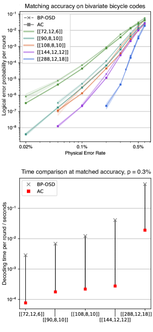
Figure 1: Top. Logical error rates for quantum memory using the bivariate bicycle codes, labelled by code parameters $[[n,k,d]]$ (the number of physical qubits, logical qubits, and the distance of the code). Syndromes were extracted for $d$ rounds; logical error and timing data are per round of syndrome extraction. Dashed lines are the BP-OSD-CS(7) (see Section 3) data from [14]. For each data point, the AC parameter $K$ (Section 4.2) has been set to match or exceed the accuracy of BP-OSD. The shaded region indicates one (binomial) standard deviation of error. Only experiments for which we observed at least 5 failures are shown. The [[108,8,10]] code is omitted for clarity as it has similar performance to the [[90,8,10]] code.  Bottom. Decoding time per round of syndrome extraction at $p=0.3\%$. Bravyi et al. only obtained BP-OSD data down to $p=0.035$ for the $[[288,12,18]]$ code so for that code we set $K$ to match accuracy based on an extrapolation.

Figure 1 shows that AC can be configured to match the logical accuracy data from [14] for the bivariate bicycle codes. (See Section 5 for details of the configuration of the decoders in each case.) We also plot the decoding times for these codes for a physical error rate of $0.3\%$ (for which BP-OSD accuracy data is available for most of the codes), with matched logical fidelities. We see a speedup of between $30\times$ and $150\times$ for the various codes. In particular, when decoding the 144-qubit Gross code at this physical error rate, we see a speedup of around $150\times$, or an absolute decoding time of 280 per round on a single CPU, with no loss of logical fidelity. This is likely already fast enough for real-time decoding on neutral atom [17] and trapped ion systems [18].

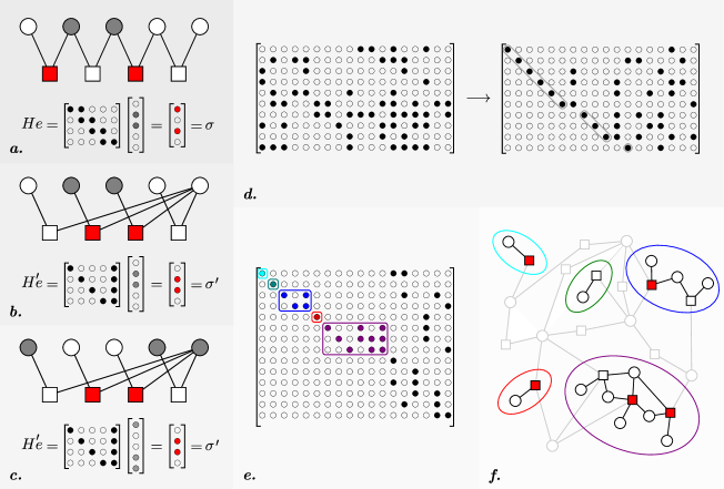
Figure 2: a. A Tanner graph for the 5-bit repetition code, with 5 error nodes (circles) and 4 check nodes (squares). Checks are each connected to an adjacent pair of error nodes, representing the condition that adjacent bits of the codewords $00000$ and $11111$ agree. An unknown error pattern (marked circles) has an observable syndrome (marked squares) consisting of the checks adjacent to an odd number of errors. Below is the associated parity check matrix $H$. The syndrome $\sigma$ is the mod 2 sum of the columns corresponding to the unknown error. Any solution $e$ to the equation $He=\sigma$ is an explanation of the observed syndrome.   b, c. A different choice of Tanner graph and the corresponding parity check matrix. The checks here represent the conditions that each bit of a codeword should agree with the final bit—an alternative way to ensure that all of the bits agree. This structure makes it particularly easy to read off the sets of columns summing to the observed syndrome: columns 2 and 3 (b), or column 5 together with columns 1 and 4 (c), corresponding to $e=(0,1,1,0,0)$ and $e=(1,0,0,1,1)$.  d. An arbitrary parity check matrix can be converted to the same special form by Gaussian elimination. Typically the parity check matrix is much wider than it is tall, so there are far more combinations of columns to search through to find the best solutions. BP-OSD streamlines this search by reordering the columns according to the output of BP, placing columns considered more likely to represent an error further to the left, before performing Gaussian elimination. High accuracy can then be obtained by searching over only small sets of columns from the right-hand side of the matrix.  e. Suppose that the parity check matrix has a partial block structure, covering the rows where the syndrome is non-zero, and that we’re confident that the rightmost block of columns corresponds to errors which did not occur. Then we can search over the possible explanations of each section of the syndrome separately. The part of the overall solution space explored by this search can be exponentially larger, in the number of blocks, than a search which does the same amount of work without regard to the block structure.  f. The blocks correspond to isolated clusters in an updated Tanner graph. The key idea of AC is that, by careful manipulation of the parity check matrix, this block structure can usually be obtained.

Figure 2 gives an overview of the decoding problem and the main innovation of AC. Information about the errors inside a quantum computer is available only indirectly, in the form of a syndrome which indicates which of some set of parity checks are violated. Each syndrome can be explained by multiple different underlying errors. The decoding problem is to map observed syndromes to the most likely underlying errors.

A decoding problem can be specified by either a Tanner graph or a parity check matrix. A Tanner graph has two types of nodes, check nodes and error nodes, with an edge between a check node and an error node whenever the corresponding check is sensitive to the corresponding error (Figure 2). The parity check matrix $H$ is the adjacency matrix of the Tanner graph: $H_{ij}$ is $1$ if the $i$th check is sensitive to the $j$th error, and $0$ otherwise. Given a syndrome $\sigma$, we seek the most likely underlying errors $e$ such that

$$He=\sigma\pmod{2}.$$ (1)

The state of the art for this problem is BP-OSD.

BP is a message-passing algorithm which uses the observed syndrome to compute an estimate of how likely each individual error is to have occurred. We can turn this into a guess for the global error pattern $e$ by setting $e_{j}=1$ precisely when BP considers that the $j$th error is more likely to have occurred than not. This is, however, a poor decoder for quantum codes, typically not even producing solutions to (1).

In contrast, when the parity check matrix is in reduced form (Figures 2, 2) it is easy to read off solutions to (1), but the number of solutions is typically exponentially large in the problem size. Ordered Statistics Decoding (OSD) uses the output of BP to direct the search to the most promising parts of the solution space.

We first sort the columns of the parity check matrix according to the output of BP, so that columns corresponding to the most likely errors are on the left of the matrix. Then we perform Gaussian elimination (see Section 3.1), proceeding left to right. This converts the matrix to reduced form (Figure 2). If the output of BP is reliable, then the best solutions to (1) will largely comprise columns in the resulting identity block, so that accurate results can be obtained by considering only relatively few combinations of the remaining columns.

Our new decoder, AC, works by producing a block structure in the parity check matrix $H$ (Figure 2), or equivalently, a cluster structure in the Tanner graph (Figure 2). This structure is obtained by modifying the Gaussian elimination algorithm to choose its next step dynamically based on the syndrome as well as the output of BP, together with a new stopping condition that prevents it from running to completion. The advantage of this block/cluster structure is twofold. First, it is much cheaper to obtain than the fully reduced form in Figure 2. Second, we can use it to search over local solutions to each cluster independently.

The remainder of the paper is set out as follows. Section 1 introduces the decoding problem. Sections 2 and 3 set the stage for a description of AC by discussing Belief Propagation, Gaussian elimination, and how they are combined in BP-OSD. In Section 4, we describe AC in full. Section 5 details the Monte Carlo simulations used to produce Figure 1.

1 The decoding problem

The Ambiguity Clustering decoder can be applied to any problem expressed in terms of parity checks on probabilistically independent error mechanisms.

Definition 1.1.

The input to a decoding problem comprises

• an $m\times n$ binary parity check matrix $H$;

• a $k\times n$ binary logical matrix $L$;

• a length $n$ vector of prior error probabilities $\epsilon$;

• a length $m$ binary syndrome vector $\sigma$.

By a binary matrix or vector we mean that the entries are in the finite field $\mathbb{F}_{2}=\{0,1\}$, with arithmetic performed modulo 2.

Given a length $n$ binary error vector $e$, write

$$\epsilon(e)=\prod_{i\colon e_{i}=1}\epsilon_{i}\cdot\prod_{j\colon e_{j}=0}(1-\epsilon_{j})$$ (2)

for the prior probability of $e$.

Definition 1.2.

The maximum likelihood decoder computes the logical effect vector $\lambda$ maximising the value of

$$\sum_{e\in\{0,1\}^{n}\colon He=\sigma,\,Le=\lambda}\epsilon(e).$$ (3)

That is, over all errors $e$ consistent with the syndrome $\sigma$, what is the most likely value of $Le$, weighted according to $\epsilon$?

For a decoding problem to be well-posed, there must be at least one $e$ such that $He=\sigma$. We will assume that the rows of $H$ are linearly independent, which guarantees that we can always find such an $e$. This simplifies the presentation, but avoids no essential difficulties, provided $\sigma$ is in the column span of $H$.

Definition 1.1 models many different types of decoding problem, such as classical linear binary codes and quantum stabiliser codes with stochastic noise and perfect measurement. Here we focus instead on quantum memory with a circuit-level noise model. We are given a circuit which initialises a block of logical qubits, implements syndrome extraction for some number of rounds, then measures off the physical qubits in such a way that the value of the logical $Z$, say, operators can be determined. In this model, $H$ and $L$ have the following interpretations.

• The errors represented by the columns of $H$ and $L$ are $n$ independent error mechanisms in the circuit, such as a particular single-qubit Pauli error on an idle qubit, a particular two-qubit Pauli error after a two-qubit gate, or an error in preparation or measurement. This $n$ will generally be many times larger than the number of physical qubits in the code.

• The checks represented by the rows of $H$ are $m$ detectors: sums (mod 2) of physical measurement results which are deterministically $0$ if no errors occur, such as measurements of the same stabiliser in consecutive rounds. The $ij$th entry of $H$ is $1$ if the value of the $i$th detector is flipped whenever the $j$th error occurs, and $0$ otherwise.

• The rows of $L$ correspond to $k$ logical observables whose values we are trying to preserve. The $ij$th entry of $L$ is $1$ if the value of the $i$th logical observable is flipped whenever the $j$th error occurs, and $0$ otherwise.

For quantum error correction $n$ is typically much larger than $m+k$, meaning that, for any $e\in\mathbb{F}_{2}^{n}$, there are a very large number (at least $2^{n-m-k}$) of $e^{\prime}$ with both $He^{\prime}=He$ and $Le^{\prime}=Le$; that is, that have an identical syndrome and logical effect. This degeneracy is a key difference between quantum and classical LDPC codes.

2 Belief Propagation and the
split belief problem

Given an observed syndrome $\sigma$, what is the updated probability that $e_{j}=1$? Belief Propagation (BP) is an efficient algorithm to produce estimates $p_{j}$ for these posterior probabilities, which works by passing messages over the associated Tanner graph.

Classical decoding problems are non-degenerate. For each logical effect $\lambda$, there is a unique error $e$ with that logical effect and the observed syndrome. Provided the most likely solution is sufficiently likely, we can find it by rounding off the posterior probabilities:

$$e_{j}=\begin{cases}0&\text{if }p_{j}<1/2,\\ 1&\text{if }p_{j}\geq 1/2.\end{cases}$$ (4)

This is not the case for quantum decoding problems. Even when there is an unambiguously most likely logical effect $\lambda$, that logical effect can be caused by many different physical errors with the observed syndrome. In this case, looking at the most likely value of each $e_{i}$ individually might not even produce an error $e$ compatible with the observed syndrome (see Figure 3). This is known as the split belief problem, and configurations leading to this situation as trapping sets [19, 20].

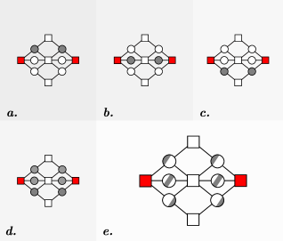
Figure 3: The split belief problem. The syndrome marked in red has four explanations a, b, c, d. If all six errors (circular nodes) have the same prior probability, then their posterior probabilities are identical (and close to $1/3$) (e). It is impossible to retrieve a solution to (1) by applying a uniform threshold to the posteriors.

Several approaches have been proposed for making effective use of BP in quantum error correction. These fall into two broad families. The first is to run BP multiple times, modifying the problem between each round, for example by modifying the prior weights $\epsilon$, the syndrome $\sigma$ or the Tanner graph itself, so that a valid global solution can be obtained [19, 21, 22, 23].

The second, and the one we take here, is to use the BP posteriors to inform a second decoding algorithm which produces the final solution. This family includes BP-OSD [12] and Belief-Matching [24, 25].

Our new decoder, AC, builds upon the ideas of BP-OSD, which we describe in some detail in the next section.

3 Gaussian elimination and BP-OSD

The state of the art for qLDPC decoding is BP with Ordered Statistics Decoding post-processing (BP-OSD). BP-OSD uses the output of BP to inform an application of Gaussian elimination, a standard procedure in linear algebra that transforms a matrix $H$ into a form particularly convenient for solving equations of the form $He=\sigma$.

Suppose that $H=\begin{bmatrix}I&B\end{bmatrix}$, where $I$ is an $m\times m$ identity matrix and $B$ is an arbitrary $m\times(n-m)$ matrix. If we write $e=\begin{bmatrix}f\\ g\end{bmatrix}$, where $f$ has length $m$ and $g$ has length $n-m$, then each of the $2^{n-m}$ solutions of

$$\sigma=He=\begin{bmatrix}I&B\end{bmatrix}\begin{bmatrix}f\\ g\end{bmatrix}=f+Bg$$ (5)

can be obtained by first choosing one of the $2^{n-m}$ values for $g$, then setting $f=\sigma+Bg$.

Definition 3.1.

A column of a matrix is in reduced form if it contains exactly one $1$. An $m\times n$ matrix as a whole is in reduced form if there is a set of $m$ columns in reduced form which have their $1$s in distinct rows.

A matrix in reduced form differs from the special form $H=\begin{bmatrix}I&B\end{bmatrix}$ only by row and column permutations, so is equally convenient for parameterising solutions to $He=\sigma$. This will be a repeating theme: a special form of $H$ will be presented with a particularly convenient ordering of the rows and columns, but any reordering of the special form will work equally well.

3.1 Gaussian elimination

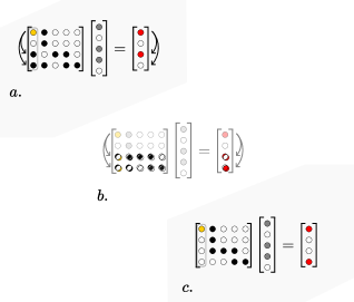
Figure 4: A pivot operation. a. A pivot $ij$ = $11$ (yellow) is chosen. b. The pivot row is added to every other row with a $1$ in the pivot column. c. The pivot column is now in reduced form. Further pivot operations in other rows will no longer change this column, so it will remain in reduced form. The syndrome vector on the right is modified in the same way to ensure the solutions (one of which is shown in grey) to the linear system are unchanged.

The basic unit of Gaussian elimination is the pivot operation (Figure 4). Choose a pivot row $i$ and pivot column $j$ of $H$ that are adjacent (meaning $H_{ij}=1$) and add the $i$th row to every other row $\ell$ adjacent to column $j$ (with $H_{\ell j}=1$). After this pivot operation, the $j$th column is in reduced form. Moreover, since the rest of the column is now $0$, further pivot operations will not take the $j$th column out of reduced form, as long as we avoid pivoting again in the same row.

The description of Gaussian elimination is now very short: for as long as we can choose a valid pivot entry $ij$ (with $H_{ij}=1$, and neither row $i$ nor column $j$ having previously been used as a pivot), pivot at $ij$. After $m$ pivot operations, $H$ will be in reduced form.

We can now decode as follows. Let $H$ be a parity check matrix, and let $H^{\prime}$ be a reduced form of $H$ obtained via Gaussian elimination. Since $H^{\prime}$ is obtained from $H$ by performing row operations, there is some invertible matrix $R$ such that $H^{\prime}=RH$. Given a syndrome $\sigma$, let $\sigma^{\prime}=R\sigma$. Then

$$He=\sigma\iff RHe=R\sigma\iff H^{\prime}e=\sigma^{\prime}$$ (6)

so we have an equivalent decoding problem to the one we started with, but where the parity check matrix is in reduced form. We can now explore the solution space to $H^{\prime}e=\sigma^{\prime}$ using the technique of (5). From now on, whenever we perform a pivot operation on $H$, we perform the same set of row operations on $\sigma$ to preserve the solution space to $He=\sigma$ (see Figure 4). We shall also omit the primes from $H^{\prime}$ and $\sigma^{\prime}$, using $H$ and $\sigma$ to refer to the current transformed state of the problem at any point.

3.2 Ordered Statistics Decoding

It generally remains impractical to iterate over all $2^{n-m}$ solutions to $He=\sigma$. A search would be much easier if the likely values of $e$ were almost entirely supported on the pivot columns. Ordered Statistics Decoding (OSD) aims to achieve this by exploiting our freedom to choose a pivot during Gaussian elimination: in each round, we select a pivot $ij$ which maximises $p_{j}$, BP’s estimate of the probability that $e_{j}=1$ given that $He=\sigma$. This is typically described as reordering the columns so that $p_{j}$ decreases left to right, then choosing the leftmost available pivot at each stage.

BP-OSD then is a family of algorithms of the following general form.

1. Obtain posterior estimates $p_{j}$ using some form of BP.

2. Perform Gaussian elimination with the pivot selection rule ‘maximise $p_{j}$’.

3. Search for a solution to the transformed problem $He=\sigma$ with highest prior probability $\epsilon(e)$.

Both the accuracy and run time can vary depending on the exact implementation of each stage. We will give a rough indication of the relative cost of each stage.

BP consists of some number of rounds $r$ passing messages along the edges of the Tanner graph. The Tanner graph has $m+n$ vertices. For a qLDPC decoding problem each vertex has bounded degree, so there are $O(m+n)=O(n)$ edges, and BP runs in time at most $O(rn)$. BP is highly amenable to parallelisation, so it is reasonable to think that this could be reduced to $O(r)$ in principle.

Gaussian elimination performs at most $m$ pivot operations, each consisting of at most $m-1$ additions of length $n$ rows, for a total complexity of $O(m^{2}n)$. The matrices involved in qLDPC decoding are sparse, so the practical complexity could be lower even if we make no special effort to use the sparsity, for example if each pivot operation involves relatively few rows.

The cost of the search stage depends heavily on how thoroughly we search. There are several named strategies in the literature [15].

• Order zero (BP-OSD-0). Take the unique solution which only uses pivot columns. That is, in the context of (5), set $g=0$.

• Exhaustive order $t$ (BP-OSD-E($t$)). Try all $2^{t}$ values of $g$ supported on the $t$ most likely non-pivot columns.

• Combination sweep order $t$ (BP-OSD-CS($t$)). Try all $g$ of weight at most $1$, and those $g$ with exactly two $1$s in positions corresponding to the $t$ most likely non-pivot columns.

Roffe et al. [15] report that combination sweep typically gives better accuracy than the exhaustive method searching a similar number of solutions. BP-OSD-CS($t$) considers $1+(n-m)+\binom{t}{2}=O(n+t^{2})$ values of $e$. Scoring each solution by computing $\epsilon(e)$ takes time $O(m)$.

For low values of $t$, Gaussian elimination is the dominant cost. For higher values of $t$, we observe that the cost of the solution search dominates.

Often $t$ is taken to be a small constant, giving satisfactory performance on small codes. However, the existence of trapping sets and the split belief problem (see Section 2) gives a heuristic argument that the amount of searching required by BP-OSD should grow exponentially in the size of the problem. If there are $s$ problematic areas of the syndrome, each of which can be resolved in at least two different ways, then an unstructured search must examine at least $2^{s}$ solutions to find the best one. But if these configurations occur at some constant rate, then for large problems $s$ will scale with $n$ for some constant fraction of syndromes supplied to the decoder.

The motivation behind AC is to try and identify and resolve these ambiguities independently, turning a multiplicative cost into an additive one.

4 Ambiguity Clustering

We now describe AC in full. Broadly speaking, AC works by performing incomplete Gaussian elimination on $H$, with modified pivot selection rules and modified stopping criteria. This has two advantages: first, it is cheaper than full Gaussian elimination. Second, the incomplete Gaussian elimination imposes a block structure on $H$, which allows for a more efficient search over the solution space.

After running BP to obtain estimated posteriors $p_{j}$, AC proceeds in three stages. In the first stage (Section 4.1), we obtain an initial solution to $He=\sigma$. In the second stage (Section 4.2), we grow outwards from this initial solution to identify additional errors, not present in the initial solution, that could be relevant to solving the decoding problem. Considering these additional errors builds a block structure in $H$, or equivalently a cluster structure in the Tanner graph. In the third stage (Section 4.3), we analyse each of the clusters separately.

We provide two figures to help the reader orient themselves. In Figure 5, we illustrate the evolution of the problem through stages 1 and  2. In Figure 7, we give a high-level overview of the algorithm.

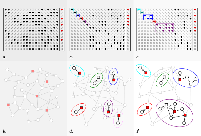
Figure 5: a. A general, unstructured, parity check matrix $H$. The syndrome $\sigma$ is shown as a column vector on its right.  b. The associated Tanner graph. Checks with a $1$ in the syndrome are marked in red.  c. After stage 1, $H$ is reduced with respect to the syndrome (Definition 4.1): an identity block covers the rows in which the syndrome has a $1$. In general, the rows and columns of the identity ‘block’ may be scattered throughout the matrix. Because a pivot row can still be involved in later pivot operations, there might (as in this example) be rows in the identity block without a $1$ in the syndrome.  d. In the Tanner graph, being reduced with respect to $\sigma$ means that every marked check has an associated error node adjacent only to that check.  e. After stage 2, an expanded set of blocks covers the syndrome. The blocks $C_{i}$ are shown as coloured rectangles. Each consists of an $m_{i}\times m_{i}$ identity matrix $I_{i}$, and optionally some linearly dependent columns in the $m_{i}\times(n_{i}-m_{i})$ matrix $B_{i}$. Again, in practice these rows and columns may be scattered throughout the matrix.  f. In the Tanner graph, each cluster consists of at least one check node–error node pair, indicated with an arrow, and optionally some additional errors adjacent only to those checks ‘gluing them together’ into a cluster. Every marked check is part of some cluster.

4.1 AC Stage 1: initial solution

Suppose that

$$H=\begin{bmatrix}I&\star\\ 0&\star\end{bmatrix}\text{ and }\sigma=\begin{bmatrix}\sigma_{1}\\ 0\end{bmatrix}$$ (7)

where $I$ is an $\ell\times\ell$ identity block, $\sigma_{1}$ has length $\ell$, a $0$ indicates a block of zeroes, and the blocks indicated by $\star$ have arbitrary entries. Then one solution to $He=\sigma$ is given by

$$e=\begin{bmatrix}\sigma_{1}\\ 0\end{bmatrix}.$$ (8)

The goal of stage 1 of AC is to bring the decoding problem into this form.

Definition 4.1.

The parity check matrix $H$ is reduced with respect to $\sigma$ if every row $i$ of the matrix with $\sigma_{i}=1$ is a pivot row.

If $H$ is reduced with respect to $\sigma$, then we have (7) up to permutations of the rows and columns. In comparison to the fully reduced form obtained in Section 3, we have done less work to find the first solution to $He=\sigma$. In return, we no longer have easy access to further solutions. Recovering these will be the purpose of stage 2.

To reduce $H$ with respect to $\sigma$, we choose pivots such that each pivot operation makes a row $i$ with $\sigma_{i}=1$ into a pivot row (possibly at the cost of creating additional $1$s in the syndrome). If we have multiple options, we break ties using the $p_{j}$ as in OSD.

Specifically, we iterate the following procedure.

1. Choose a pivot row $i$ and pivot column $j$ according to the following criteria:

   1. the two must be adjacent ($H_{ij}=1$);

   2. neither has previously been used as a pivot;

   3. the row must have a non-zero syndrome ($\sigma_{i}=1$); and

   4. of the pairs $ij$ satisfying (a), (b) and (c), choose a pair with maximal $p_{j}$.

2. Perform a pivot operation using pivot row $i$ and pivot column $j$, updating both $H$ and $\sigma$ to preserve the solution space of $He=\sigma$.

3. Repeat steps 1 and 2 until there are no more pairs satisfying (a), (b) and (c), at which point $H$ will be reduced with respect to $\sigma$.

The key difference from OSD is in condition 1(c). In OSD, the order in which pivots are chosen is fixed in advance. By contrast, here we select the next pivot dynamically based on both $p_{j}$ and the current state of the updated syndrome. Since the original syndrome is sparse, this condition and the associated early-stopping behaviour allow the initial solution to be obtained much more quickly than in BP-OSD.

4.2 AC stage 2: cluster formation

In stage 2 we transform the matrix $H$ into its final form, a block structure that captures the local structure of the solution space. The blocks can also be viewed as clusters in a Tanner graph.

The block form we are aiming for is, up to row and column permutations,

$$H=\begin{bmatrix}C&\star\\ 0&\star\end{bmatrix},$$ (9)

where

$$C=\begin{bmatrix}I&B_{1}&&&\\ &&\ddots&&\\ &&&I&B_{c}\end{bmatrix}.$$ (10)

An example matrix of this form is shown in Figure 5. If we reinterpret $C$ as the adjacency matrix of a Tanner graph, the $c$ blocks correspond to connected components. Figure 5 shows these connected components embedded inside the full Tanner graph represented by $H$.

Writing

$$C_{i}=\begin{bmatrix}I&B_{i}\end{bmatrix},$$ (11)

each $C_{i}$ is an $m_{i}\times n_{i}$ matrix in reduced form. Suppose that

$$\sigma=\begin{bmatrix}\sigma_{1}\\ \vdots\\ \sigma_{c}\\ 0\end{bmatrix},$$ (12)

with each $\sigma_{i}$ of length $m_{i}$. If we let

$$e=\begin{bmatrix}e_{1}\\ \vdots\\ e_{c}\\ 0\end{bmatrix},$$ (13)

with each $e_{i}$ of length $n_{i}$, then $He=\sigma$ if and only if

$$C_{i}e_{i}=\sigma_{i}$$ (14)

for each $i$. The condition (13) is reasonable provided the zero block corresponds to error mechanisms that are unlikely to have occurred. As long as we can ensure this, we will have split the decoding problem into many smaller decoding problems that can be solved separately.

The partially reduced form (7) can be viewed as a trivial example of this block structure with $C$ consisting of the pivot rows and columns, with $m_{i}=n_{i}=1$ throughout. In stage 2 we will add an additional $K$ columns to $C$, and typically also some rows. Increasing $K$ increases the accuracy of the decoder at the cost of increased run time.

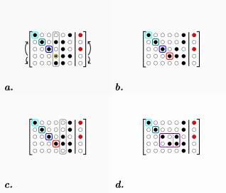
Figure 6: The two stage 2 operations. a. The selected column has a $1$ in a non-pivot row. b. We perform a pivot operation and seed a new block (red). c. The selected column is supported on pivot rows. d. We add the column to $C$ unchanged, merging blocks (purple) as necessary.

When we add a column $j$ to $C$, one of two things happens, depending on the relationship between that column and $C$ (Figure 6).

Seed a new block. If column $j$ has at least one $1$ outside the rows of $C$, choose such a row $i$ arbitrarily and pivot at $ij$. The resulting column $j$, containing only a single $1$, can be added as a new block of $C$. The number of rows, columns and blocks of $C$ each increase by $1$.

Grow existing blocks. Otherwise, column $j$ is supported entirely on the rows of $C$, so we can add it to $C$ unchanged. It is possible that column $j$ has $1$s in several different blocks of $C$. In that case, we merge those blocks into a single larger block. The number of rows is unchanged, the number of columns increases by 1, and the number of blocks either stays the same or decreases.

Stage 2 proceeds as follows.

1. Choose a column $j$ that

   1. is not in $C$;

   2. is adjacent to a row that has been involved in a pivot operation in stage 1 or stage 2 (either as a pivot row, or by having a pivot row added to it); and

   3. has maximal $p_{j}$ among those columns satisfying (a) and (b).

2. Add column $j$ to $C$, either by seeding a new block or growing existing blocks as appropriate.

3. Repeat steps 1 and 2 until a total of $K$ additional columns have been added to $C$.

The goal of step 1 is to select the column most likely to be involved in solutions to $He=\sigma$. This ensures that it is reasonable to restrict attention to $e$ of the form (13), allowing us to solve many small systems (14) separately.

4.3 AC stage 3: cluster analysis

So far, nothing has depended on the logical matrix $L$. Returning $L$ to the picture, at the end of stage 2 we have (up to row and column permutations)

$$H =\begin{bmatrix}C_{1}&&&\star\\ &\ddots&&\vdots\\ &&C_{c}&\star\\ 0&\cdots&0&\star\end{bmatrix} \sigma=\begin{bmatrix}\sigma_{1}\\ \vdots\\ \sigma_{c}\\ 0\end{bmatrix}$$ (15)

$$L =\;\begin{bmatrix}L_{1}&\cdots&L_{c}&\star\end{bmatrix}$$

where we have labelled by $L_{i}$ the part of $L$ restricted to the columns in block $C_{i}$, and are promising to make no further use of the starred columns.

The triples $C_{i},\sigma_{i},L_{i}$ express smaller decoding problems which we shall solve separately. It turns out that many of these problems are very easy.

4.3.1 Unambiguous clusters

The maximum likelihood solution to the $i$th cluster is the $\lambda_{i}$ maximising

$$\sum_{e_{i}\in\{0,1\}^{n_{i}}\colon C_{i}e_{i}=\sigma,\,L_{i}e_{i}=\lambda_{i}}\epsilon_{i}(e_{i}).$$ (16)

where $\epsilon_{i}(e_{i})$ denotes the restriction of (2) to just those columns in $C_{i}$.

It turns out that there is frequently only a single value of $\lambda$ for which (16) is non-zero. That is, there is only a single logical effect consistent with the local syndrome, once we have committed to explaining that part of the syndrome locally. This is analogous to the neutral clusters arising during execution of the Union-Find decoder [6]: all corrections within a cluster are logically equivalent, so we can choose between them arbitrarily (for example, by ‘peeling’ in Union-Find).

Unambiguous clusters occur precisely when each row of $L_{i}$ is linearly dependent on the rows of $C_{i}$. In that case there is some $k\times m_{i}$ matrix $R_{i}$ such that $L_{i}=R_{i}C_{i}$, so that

$$\lambda_{i}=L_{i}e_{i}=R_{i}C_{i}e_{i}=R_{i}\sigma_{i}$$ (17)

for every $e_{i}$ with $C_{i}e_{i}=\sigma_{i}$; that is, the logical effect $\lambda_{i}$ is a linear function of the syndrome $\sigma_{i}$.

Unambiguous clusters can be detected efficiently: since $C_{i}$ is in reduced form,

$$R_{i}C_{i}=R_{i}\begin{bmatrix}I&B_{i}\end{bmatrix}=\begin{bmatrix}R_{i}&R_{i}B_{i}\end{bmatrix},$$ (18)

which can only possibly equal $L_{i}$ for a single choice of $R_{i}$, which is easily checked.

4.3.2 Ambiguous clusters

In many cases, all clusters arising from stage 2 are unambiguous and no further analysis is necessary. When there is at least one ambiguous cluster, we have typically observed exactly one.

The ambiguous clusters are smaller than the original decoding problem, but are still generally too large to allow the maximum likelihood decoding problem to be solved exactly. We therefore adopt a restricted search strategy, analogous to the search in the final stage of OSD.

As in Section 3.1, we let $e_{i}=\begin{bmatrix}f_{i}\\ g_{i}\end{bmatrix}$, with $f_{i}$ of length $m_{i}$ and $g_{i}$ of length $n_{i}-m_{i}$ so that the $2^{n_{i}-m_{i}}$ solutions to

$$\sigma_{i}=C_{i}e_{i}=\begin{bmatrix}I&B_{i}\end{bmatrix}\begin{bmatrix}f_{i}\\ g_{i}\end{bmatrix}=f_{i}+B_{i}g_{i}$$ (19)

are given by choosing any value for $g_{i}$ and letting $f_{i}=\sigma_{i}+B_{i}g_{i}$. Then we try the solutions given by every $g_{i}$ of weight up to $2$. (Note that BP-OSD-CS tries only a subset of the weight-2 solutions available to it.) For each solution, we calculate $\epsilon_{i}(e_{i})$. We track the sum of probabilities associated with solutions which flip, and the sum of probabilities of solutions which do not flip, each logical observable $j$. If the former sum is greater than the latter, we determine the cluster to have flipped the logical, and we set the $j$th bit of $\lambda_{i}$ to $1$; otherwise, we set it to $0$.

4.3.3 Combining cluster results

For each cluster $C_{i}$, ambiguous or not, we have now calculated an estimate $\lambda_{i}$ for the logical effect of the errors associated with that cluster. The estimated total logical effect returned by the decoder is $\lambda=\sum_{i=1}^{c}\lambda_{i}$.

Analysing each cluster separately is very efficient. Considering $s_{i}$ solutions for each cluster $C_{i}$ has a cost scaling with $\sum_{i=1}^{c}s_{i}$ but covers a part of the solution space to the original decoding problem of size scaling like $\prod_{i=1}^{c}s_{i}$. This is part of what allows us to achieve the accuracy of BP-OSD at much lower computational cost.

4.4 Summary of stages of AC

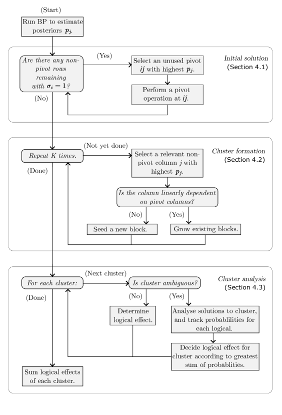
Figure 7: Schematic overview of AC.

To summarise, AC has four stages, depicted in Figure 7:

• Run BP on the syndrome to obtain posterior probability estimates $p_{j}$.

• AC stage 1, initial solve. Informed by the syndrome and the BP posteriors, perform pivot operations to put the matrix $H$ into reduced form, sufficient to identify one solution.

• AC stage 2, cluster formation. Perform further pivot operations and include linearly dependent errors to form a block structure.

• AC stage 3, cluster analysis. For each logically ambiguous cluster, analyse a subset of the solutions to determine its likely logical effect, and sum these together with the effects of the unambiguous clusters to obtain a final overall logical effect.

5 Numerical methods

Bravyi et al. [14] described circuits to perform syndrome extraction for their codes. We use versions of these circuits made available by Gong et al. [23] for Gidney’s Clifford simulator Stim [26]. The circuits describe the preparations, gates and measurements for a quantum memory experiment: initialise a block of qubits, extract $r$ rounds of measurement data, then measure the physical qubits to determine the error states of the $k$ logical $Z$ observables.

We use the same circuit-level noise model as [14] with a single parameter $p$.

• State preparation. With probability $p$, prepare the orthogonal state (e.g. $\ket{1}$ instead of $\ket{0}$).

• Measurement. With probability $p$, flip the classical measurement result (from $0$ to $1$ or vice versa).

• After single qubit gates. With probability $p$, apply Pauli $X$, $Y$ or $Z$ with equal probability. (This is equivalent to depolarising the qubit with probability $4p/3$.) An idle qubit in any time step experiences a noisy identity gate.

• After two qubit gates. With probability $p$, apply one of the $15$ non-trivial 2-qubit Pauli operations $IX$, $IY$, $IZ$, $XI$, etc. (This is equivalent to depolarising both qubits with probability $16p/15$.)

Stim performs two functions. First, it analyses the circuit to produce a ‘detector error model’, which contains information equivalent to the parity check matrix $H$, logical matrix $L$ and prior probabilities $\epsilon$. Second, it efficiently simulates the noisy syndrome extraction circuit, producing syndrome data and associated true logical effects against which we can assess the accuracy of a decoder.

The codes we test against encode more than one logical qubit. We count as a failure any run of the decoder in which we do not compute the full logical state correctly. We report the per-round logical failure rate

$$p_{\text{fail}}=\frac{f}{rN}$$ (20)

where $N$ is the number of calls to the decoder, $f$ is the number of decoding failures, and $r$ is the number of rounds of syndrome extraction (in all cases set equal to the reported distance of the code). This formula ignores the second order effects of cancelling logical errors. These effects are more complicated to analyse for codes encoding multiple logical qubits than for those with a single logical qubit, but also less likely. The per-round logical failure rate for BP-OSD was computed in the same way from data kindly provided by the authors of [14].

Timing data for both AC and BP-OSD were obtained by running each single-threaded on an M2-based MacBook Pro. We used a common Python harness that generates syndrome data using Stim then calls out to either our C++ implementation of AC, or the standard BP-OSD implementation by Roffe [15, 16] in Cython. Only time spent in the decoder is included in the reported per-round timing data.

Both AC and BP-OSD are families of decoding algorithms with various adjustable parameters.

In AC, we set

1. the number of rounds of (sum-product) BP equal to the distance of the code;

2. the number $K$ of additional columns added to $C$ in stage 2 to match or exceed the accuracy of BP-OSD on each data point in Figure 1. We took $K=\kappa n$, where $n$ is the number of columns in the parity check matrix, and tried $\kappa$ from $0$ to $0.1$ in steps of $0.01$.

To collect the timing data for BP-OSD we set

1. the number of rounds of (min-sum) BP equal to the distance of the code;

2. the combination sweep order $t$ equal to $7$.

In the repository [27] associated to [14], Bravyi et al. use $t=7$ and 10 000 rounds of BP; obtaining the timing data with the reduced number of rounds is slightly favourable to BP-OSD.

References

- [1] Nick S. Blunt, Joan Camps, Ophelia Crawford, Róbert Izsák, Sebastian Leontica, Arjun Mirani, Alexandra E. Moylett, Sam A. Scivier, Christoph Sünderhauf, Patrick Schopf, Jacob M. Taylor, and Nicole Holzmann. Perspective on the current state-of-the-art of quantum computing for drug discovery applications. Journal of Chemical Theory and Computation, 18(12):7001–7023, 2022. PMID: 36355616.
- [2] Nathalie P. de Leon, Kohei M. Itoh, Dohun Kim, Karan K. Mehta, Tracy E. Northup, Hanhee Paik, B. S. Palmer, N. Samarth, Sorawis Sangtawesin, and D. W. Steuerman. Materials challenges and opportunities for quantum computing hardware. Science, 372(6539):eabb2823, 2021.
- [3] P.W. Shor. Algorithms for quantum computation: discrete logarithms and factoring. In Proceedings 35th Annual Symposium on Foundations of Computer Science, pages 124–134, 1994.
- [4] A. Yu Kitaev. Quantum computations: algorithms and error correction. Russian Mathematical Surveys, 52(6):1191–1249, December 1997.
- [5] Jack Edmonds. Paths, trees, and flowers. Canadian Journal of Mathematics, 17:449–467, 1965.
- [6] Nicolas Delfosse and Naomi H. Nickerson. Almost-linear time decoding algorithm for topological codes. Quantum, 5:595, December 2021.
- [7] Nikolas P. Breuckmann and Jens Niklas Eberhardt. Quantum low-density parity-check codes. PRX Quantum, 2:040101, Oct 2021.
- [8] Jean-Pierre Tillich and Gilles Zemor. Quantum ldpc codes with positive rate and minimum distance proportional to n½. In 2009 IEEE International Symposium on Information Theory, pages 799–803, 2009.
- [9] Anthony Leverrier, Jean-Pierre Tillich, and Gilles Zémor. Quantum expander codes. In 2015 IEEE 56th Annual Symposium on Foundations of Computer Science, pages 810–824, 2015.
- [10] Pavel Panteleev and Gleb Kalachev. Asymptotically good quantum and locally testable classical ldpc codes. In Proceedings of the 54th Annual ACM SIGACT Symposium on Theory of Computing, STOC 2022, page 375–388, New York, NY, USA, 2022. Association for Computing Machinery.
- [11] Sergey Bravyi, David Poulin, and Barbara Terhal. Tradeoffs for reliable quantum information storage in 2d systems. Phys. Rev. Lett., 104:050503, Feb 2010.
- [12] Pavel Panteleev and Gleb Kalachev. Degenerate quantum LDPC codes with good finite length performance. Quantum, 5:585, November 2021.
- [13] Yifei Shen, Wenqing Song, Yuqing Ren, Houren Ji, Xiaohu You, and Chuan Zhang. Enhanced belief propagation decoder for 5G polar codes with bit-flipping. IEEE Transactions on Circuits and Systems II: Express Briefs, 67(5):901–905, 2020.
- [14] Sergey Bravyi, Andrew W. Cross, Jay M. Gambetta, Dmitri Maslov, Patrick Rall, and Theodore J. Yoder. High-threshold and low-overhead fault-tolerant quantum memory. Nature, 627(8005):778–782, 2024.
- [15] Joschka Roffe, David R. White, Simon Burton, and Earl Campbell. Decoding across the quantum low-density parity-check code landscape. Phys. Rev. Res., 2:043423, Dec 2020.
- [16] Joschka Roffe. LDPC: Python tools for low density parity check codes, 2022. https://pypi.org/project/ldpc/.
- [17] C. Poole, T. M. Graham, M. A. Perlin, M. Otten, and M. Saffman. Architecture for fast implementation of qLDPC codes with optimized Rydberg gates, 2024.
- [18] Fangzhao Alex An, Anthony Ransford, Andrew Schaffer, Lucas R. Sletten, John Gaebler, James Hostetter, and Grahame Vittorini. High fidelity state preparation and measurement of ion hyperfine qubits with . Phys. Rev. Lett., 129:130501, Sep 2022.
- [19] D. Poulin and Y. Chung. On the iterative decoding of sparse quantum codes. Quantum Information and Computation, 8:986–1000, 11 2008.
- [20] Nithin Raveendran and Bane Vasić. Trapping sets of quantum LDPC codes. Quantum, 5:562, October 2021.
- [21] Julien du Crest, Francisco Garcia-Herrero, Mehdi Mhalla, Valentin Savin, and Javier Valls. Check-agnosia based post-processor for message-passing decoding of quantum LDPC codes. Quantum, 8:1334, May 2024.
- [22] Julien du Crest, Mehdi Mhalla, and Valentin Savin. Stabilizer inactivation for message-passing decoding of quantum LDPC codes, 2023.
- [23] Anqi Gong, Sebastian Cammerer, and Joseph M. Renes. Toward low-latency iterative decoding of QLDPC codes under circuit-level noise, 2024.
- [24] Ben Criger and Imran Ashraf. Multi-path summation for decoding 2D topological codes. Quantum, 2:102, October 2018.
- [25] Oscar Higgott, Thomas C. Bohdanowicz, Aleksander Kubica, Steven T. Flammia, and Earl T. Campbell. Improved decoding of circuit noise and fragile boundaries of tailored surface codes. Phys. Rev. X, 13:031007, Jul 2023.
- [26] Craig Gidney. Stim: a fast stabilizer circuit simulator. Quantum, 5:497, July 2021.
- [27] Sergey Bravyi. BivariateBicycleCodes, 2024. https://github.com/sbravyi/BivariateBicycleCodes.