Abstract

Recently, large language models (LLMs) have shown surprising performance in task-specific workloads as well as general tasks with the given prompts. However, to achieve unprecedented performance, recent LLMs use billions to trillions of parameters, which hinder the wide adaptation of those models due to their extremely large compute and memory requirements. To resolve the issue, various model compression methods are being actively investigated. In this work, we propose SDQ (Sparse Decomposed Quantization) to exploit both structured sparsity and quantization to achieve both high compute and memory efficiency. From our evaluations, we observe that SDQ can achieve 4$\times$ effective compute throughput with $<$1% quality drop.

1 Introduction

Large Language Models (LLMs) Brown et al. (2020); Chowdhery et al. (2022); Touvron et al. (2023b) with billions or trillions of parameters have gained extensive attention as they show promising quality in various domains. With such popularity, efficiently deploying and accelerating LLMs are the utmost research question for system designers, as the large number of weights causes a huge memory footprint and an enormous amount of computations. To address this issue, recent work has applied various model compression methods, such as sparsification Frantar & Alistarh (2023) and quantization Dettmers et al. (2022), on LLMs to reduce memory footprint and computations. However, when compared to classic DNN models (ResNet, BERT), LLMs introduce new challenges to both sparsification and quantization.

Model sparsification, such as model pruning LeCun et al. (1989); Han et al. (2015), reduces the target model size by removing parameters in weights and storing the weights using a compressed format. Sparsity not only reduces the memory requirement but also enables performance improvement and power saving by skipping ineffectual computation, i.e., $0\times X=0$. Exploiting this opportunity, recent NVIDIA Ampere GPU systems provide native support for 2:4 structured sparsity, a specialized form of sparse pattern that guarantees $2\times$ computation reduction and performance gain with low overhead, i.e., sparsity tax Wu et al. (2023).

Although many sparsification methods have been proposed for the classic DNNs, these techniques are less successful so far to compress LLMs. Previous efforts Hoefler et al. (2021) have shown how to compress classic DNNs by more than 90% (10$\times$ computation reduction) with limited loss of model quality; however, when it comes to LLMs, compressing beyond 50% (2$\times$ computation reduction) with a limited loss of accuracy is already challenging Frantar & Alistarh (2023); Sun et al. (2023) as shown in Figure 1.

On the other hand, quantization reduces the target model size by using a narrower bit width per value. For example, if we use an 8-bit or a 4-bit format instead of a 16-bit format for each parameter, we can reduce the model size by half and a quarter, respectively. Furthermore, when quantization is applied to both weights and activations, we can use specialized, low-bit-width arithmetic computation instead of full-precision computation, which is both more power-efficient and area-efficient Horowitz (2014); van Baalen et al. (2023). As the low-bit-width arithmetic unit takes a smaller area, processors with a given area budget for compute units could allocate more low-bit-width compute units. For example, in NVIDIA Ampere GPU, the peak tensor throughput for int8 format is 2$\times$ of the peak throughput for fp16 (4$\times$ for int4 format).

Like sparsification, quantization also faces new challenges with LLMs. While prior work has shown how to use various 4-bit formats Dai et al. (2021); Darvish Rouhani et al. (2023) for classic models, limited work shows how to quantize both activation and weights of LLMs to 4-bit format to leverage the high throughput, low-bit-width hardware units. Recent work Guo et al. (2023); Lin et al. (2023) has shown that outliers in activations obstruct quantizing both activations and weights as it causes high quantization error, which results in a huge error in the final output when propagated. Various work in this area instead focuses on 8-bit dual quantization Dettmers et al. (2022), or quantization for weights only Lin et al. (2023); Dettmers et al. (2023), limiting the computation reduction to be up to 2$\times$.

Figure 1: Effective compute throughput and perplexity increase comparison of sparsification-only, quantization-only, and SDQ on OPT-6.7B and LLaMA-7B.

In this paper, we demonstrate how to achieve even larger computation reduction (more than 2$\times$) by combining sparsification and quantization. Our key insight is that sparsification could be used to complement the outlier problem in the LLM quantization while maintaining high throughput with a low overhead using the structured sparsity patterns. Based on the insight, we propose a hybrid model compression method leveraging both sparsification and quantization to further increase computation reduction, while maintaining model quality through decomposing weights into structured sparse tensors and using structured sparse/low-bit-width compute HW. We focus on post-training model compression, which does not require any model retraining or fine-tuning as training LLMs could be infeasible in many cases (due to limited compute resources or data).

We summarize our contribution in the following:

• We illustrate the opportunity to treat the outliers during quantization as structured sparse tensors to accelerate with structured sparse HW.

• We propose SDQ, a technique to combine both sparse and quantization emerging hardware support. It achieves a better Pareto curve in model quality and compute throughput than sparsification-only or quantization-only methods.

• We show that SDQ is orthogonal to sparsification and quantization techniques. With an improved sparsified or quantized model, SDQ would also perform better.

2 Background

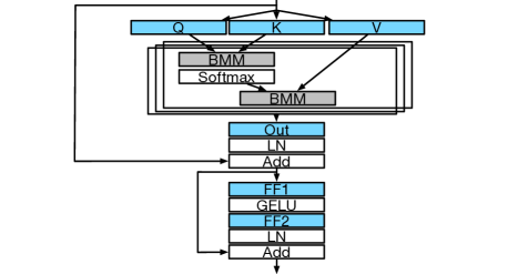
Figure 2: A transformer block architecture.

2.1 Compressing LLM models

In Figure 2, we show a high-level overview of decoder-only Transformer block architecture used in the recent LLMs. Each Transformer block contains multiple layers including linear layers, activation layers, normalization layers, etc., and the layers colored with blue and grey in Figure 2 contribute to $>$99% of the computations during inference. Linear layers (Q, K, V, out, FF1, and FF2) consist of matrix-matrix multiplications (GEMMs) with static weights, while self-attention layers ( BMMs) consists of GEMMs with dynamic activations. While the actual computation breakdown depends on the input context sizes, as well as the model parameters, generally speaking, GEMMs from the linear layers dominates the overall computation and latency Vaswani et al. (2017). As the result, in this paper, we consider model optimization and compression for only the GEMMs for the linear layers (blue layers with static weights).

	Sparsification	Quantization	Outlier	Compute	Compute
	Configuration	Configuration	Extraction	Cores	Bit Width
ASP Pool et al. (2021)	2:4	X	X	2:4 Sparse TC	16b
WANDA Sun et al. (2023)	2:4	X	X	2:4 Sparse TC	16b
VS-Quant Dai et al. (2021)	X	W4-8A4-8	X	TC	4b/8b
AWQ Lin et al. (2023)	X	W3-4A16	X	TC	16b
SparseGPT Frantar & Alistarh (2023)	2:4/4:8	W4A16	X	2:4 Sparse TC	16b
LLM.int8() Dettmers et al. (2022)	Unstr. 0.1%	W8A8	O	TC + CUDA Core	8b
SpQR Dettmers et al. (2023)	Unstr. 1%	W3-4A16	O	TC + CUDA Core	16b
OWQ Lee et al. (2023)	Col-wise $<$1%	W3-4A16	O	TC + CUDA Core	16b
SqueezeLLM Kim et al. (2023)	Unstr. $<$1%	W3-4A16	O	TC + CUDA Core	16b
SDQ (Our Work)	N:4/N:8	W4A4/W8A8	O	Flexible Sparse TC	4b/8b

Table 1: Summary of related work on sparsification and quantization. TC means Tensor Core and Unstr. means Unstructured sparsity.

2.2 Sparification

Sparsification induces sparsity in tensors, i.e. making some non-zero elements to zeros. The most popular sparsification technique used for DNNs is weight pruning which statically removes non-zero weight values by setting them zeros. Pruning DNN models is effective for classic DNNs as they are often overly parameterized, so removing insignificant values would not impact model quality when done carefully.

The simplest way to perform pruning is by choosing insignificant values based on the magnitudes Han et al. (2015) as shown in Figure 3, but previous work has proposed various metrics to decide how to choose values to be removed. For example, some methods leverage input samples and use the first order error Molchanov et al. (2022) during inference to determine which weigh value can be pruned with minimal error. Other method proposes to use second order error (Hessian) Frantar & Alistarh (2023) to predict impact of weight pruning more accurately, but at a higher computation cost, since calculating the Hessian matrix is non-trivial. While these pruning methods uses different metrics, they are very successful in compressing the conventional DNN models: many of them show possibility to compress more than 10$\times$.

Unlike a plethora of work on sparsifying conventional DNNs such as CNNs, there is a still limited number of work on sparisfying LLMs due to two major challeneges. First, LLMs are usually less over-parameterized Chowdhery et al. (2022) than the classic models. Therefore, most of the weight values are relatively crucial and cannot be pruned without impacting the model quality. Second, LLMs have much larger total parameter counts, which leads to even higher computation costs to apply first- and second-order method for pruning.

Most recently, Wanda Sun et al. (2023) and SparseGPT Frantar & Alistarh (2023) shows how to avoid the expensive computation to prune LLMs and successfully demonstrate a family of pruned LLM models. OWL Yin et al. (2023) improves on these techniques with an outlier-aware and non-uniform layer pruning. However, all of them can only prune and compress the model by about 2$\times$ without significant impacting the model quality. As we will see in later sections, compressing LLMs with pruning is still challenging.

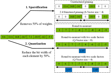
Figure 3: Overview of sparsification and quantization.

2.3 Quantization

Quantization is another popular method for DNN compression. Contrary to sparsification, quantization aims to represent “all” values in a tensor with a lower-bit-width format. Since most models can be trained with fp16 computation, deploying the trained model and performing inference with fp16 is the natural extension. As many researchers have found out Dai et al. (2021), once a model is trained, representing the weight value in lower-bit-width does not impact the model quality much. For example, an original value in a higher precision can be rounded to the nearest (RTN) lower precision value as shown in Figure 3. Besides the bit width of the quantization format, it is also crucial to decide the target for the quantization: weights and/or activations. When quantization is applied to both weights and activations, it reduces the cost of required hardware unit and enables the exploitation of simpler arithmetic computations with low-bit-width compared to the fp16 computations, which saves area and power and increases compute throughput. As a result, commercial products NVIDIA (2020; 2022) have included fp8 and int8 computation support with a higher peak computation throughput for inference.

Similar to classic DNNs, LLMs can be quantized to lower bit precision such as int8 or fp8 after training. Previous work Dettmers et al. (2022) shows how to quantize both weights and activations of LLMs with int8 (W8A8) and leverage 8-bit matrix multiplication unit in modern hardware. On the other hand, other work such as GPTQ Frantar et al. (2023) or AWQ Lin et al. (2023) focus on weight-only quantization to minimize the memory footprint of weights while keeping activations as is. Both GPTQ and AWQ show that it is able to quantize weights to 4 bits while maintaining the quality of LLMs (W4A16). Although they reduce the bit width of weights aggressively, the weights are converted back to fp16 and use lower-throughput fp16 hardware units during the inference as activations are not quantized.

An important problem in LLM quantization, as pointed out by recent work Dettmers et al. (2022), is that the quantization error becomes large due to a few outliers in activations, especially for the large models. These outliers, by definition, are often a very small portion ($<10\%$) of the activation tensors. Also, there are some sensitive values that would affect significantly to the final outcome. As these values require to be stored and compute in a higher precision, computation savings with quantization is capped at 2$\times$ at most (fp16 into fp8/int8).

Table 1 compares the mentioned prior work above, and our proposed method SDQ. Unlike the previous works, our method uses structured sparse decomposition with different bit widths to achieve 4$\times$ compute throughput.

3 Comparing Compression Methods

Since LLM inference stresses the system in various ways (computation, memory capacity, etc.), different compression methods often target different goals to optimize. In this section, we define a few metrics that can be used to estimate the computation and memory capacity savings for each method and highlight the critical design choices for them.

3.1 Effective compute throughput for sparsification

When multiplying a weight matrix with an activation matrix, if there is overall 90% unstructured sparsity in weights, the required number of Multiply–Accumulate (MAC) operations can be reduced by 90% by skipping ineffectual computations. However, identifying effectual computations and only mapping them to the compute unit (e.g., tensor cores) is not trivial, so it is difficult to exploit unstructured sparsity without investing significant area and power Qin et al. (2020). To mitigate the problem, recent work from both industry and academia Zhu et al. (2019); NVIDIA (2020); Jeong et al. (2023) propose to use N:M structured sparsity (at most N non-zero values in each consecutive M values, as shown in Figure 3), which provides predictable compute throughput while exploiting sparsity for higher performance. For example, with NVIDIA Ampere sparse tensor core, using 2:4 structured sparsity can reduce 50% of the required number of MAC operations by skipping ineffectual computations. Using the 1:8 structured sparsity in an emerging Sparse Tensor Core Liu et al. (2021); Jeong et al. (2023) can reduce up to 87.5%. Generally, using N:M structured sparse hardware support, one can reduce the required computation by $\frac{M-N}{M}\times 100$%) and increase the throughput respectively.

In this work, we focus on using a futuristic, N:M structured sparse tensor core support that can provide $\frac{M}{N}\times$ compute throughput for N:M structured sparsity, which is more practical and realistic.

3.2 Effective compute throughput for quantization

On the other hand, unlike sparsification, quantization methods are not directly used to reduce the number of MAC operations as there is no ineffectual computation after quantization. However, if both weights and activations are quantized, the low-bit-width computation unit (e.g., INT8 Tensor Core) can be used, which is more efficient compared to the full-precision computation unit. Thus, given the same area/power budget, the number of low-bit arithmetic units would be higher than that of high-bit arithmetic units, but the exact ratio could vary depending on the actual implementation. As mentioned earlier, the compute throughput of 4bit and 8bit format is 4$\times$ and 2$\times$ compared to that of the 16bit format, respectively in NVIDIA Ampere GPU NVIDIA (2020).

In this work, we assume fp16 as the baseline format for LLM inference, so we assume $\frac{16}{n}\times$ compute throughput can be achieved when both operands are quantized to $n$-bit for computations.

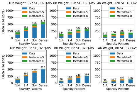
Figure 4: Data size for 32 elements with 1:4/2:4/3:4/Dense sparsity with quantization using 1) 32 bit scale factor with Q-Vector size of 16 (first row) 2) 8 bit scale factor with Q-Vector size of 32 (second row). SF and Q-VS represent Scale Factor and Q-Vector Size.

3.3 Average bits per weight element

The improved effective compute throughput mentioned above do not come for free. To maximize the advantage of sparsification, weights are often stored in a compressed format, such as bitmask, ELLPACK, CSR, etc. A compressed format usually requires both data (for the actual non-zero values) and metadata (for the indexes of non-zero values). Thus, the overhead in terms of memory is metadata to store the indexes of non-zero values. In Figure 3, we show how a simple vector composed of 8 values can be sparisfied to a vector with 2:4 structured sparsity. For N:M sparsity, we call M as the size of the S-Vector, so in this case, 4 is the size of the S-Vector. Both N and M could affect the size of the metadata. For example, if we use ELLPACK-like format that stores indexes of non-zero elements in a vector, 2:4 sparsity requires 2 bits per index ($log_{2}4$) for each non-zero value, so $2\times 2=4$ bits per vector, while 1:8 sparsity requires 3 bits per index ($log_{2}8$) for each non-zero value, so $3\times 1=3$ bits per vector.

For quantization, the overhead that needs careful consideration is caused by scale factors. In Figure 3, three different quantization method is used; round-to-neareast, round-to-nearest with a global scale factor, and round-to-nearest with per-vector scale factor (we call this as Q-Vector to distinguish with S-Vector). A scale factor is used to match the range of quantized values and the range of the original values. For example, without using a scale factor, all the values larger than 8 in Figure 3 will be quantized to 8, which could cause a significantly large quantization error. As the finer granularity of the scale factor can provide more tuned quantization, it is better to have a smaller Q-Vector size for reducing quantization error. However, similar to the indexes for compressed format, scale factors are the metadata for quantization. For example, assume a case where a value is quantized from 16-bit to 4-bit while a scale factor is 16-bit, and Q-Vector size is 4. For each vector, the data size would be $4\times 4=16$ bits while the metadata size is also 16 bits as the size of a scale factor is 16-bit (in this case, average bits per weight element would be $\frac{16+16}{4}=8$ bits). Thus, scale factors are often also quantized and Q-Vector size is kept relatively large (16-64) Dai et al. (2021).

In Figure 4, we show how much portion the size of metadata for sparsification (Metadata-S) and metadata for quantization (Metadata-Q) would take compared to the size of the actual data, showing that the metadata overhead caused by quantization and sparsification needs to be carefully considered as it could nullify the benefits of the optimization methods. For example, a 3:4 sparse, 4-bit quantized model can have a higher bit-per-weight than a dense, 4-bit quantized model.

4 SDQ: Tackling Challenges in LLM Compression with a Hybrid method

In Table 1, we summarize the previous work related to sparsification and quantization for LLMs. The first observation from sparsification perspective is that even though 2:4/4:8 sparsity would provide 2$\times$ effective compute throughput, it is hard to use for LLMs Sun et al. (2023); Frantar & Alistarh (2023) while maintaining the quality of the model (less than 1% quality drop). We observed that even with the state-of-the-art sparsification methods, 2:4/4:8 sparsity on OPT-350M cause 77%/142% perplexity increase when evaluation with raw-Wikitext2 as shown in Table 2. Even though the larger models are more tolerant than small models, inducing 2:4/4:8 sparsity on the OPT-175B model (the largest public model) still causes 3$-$6% perplexity increase, which is significant considering that only 1% is acceptable by MLPerf benchmarking rules Reddi et al. (2020). Also, even if 3$-$6% perplexity increase is acceptable, it can only achieves 2$\times$ effective compute throughput.

The second observation is that the previous work focusing on weight-only quantization is able to reduce the weight bit width to 4 bit while dual quantization can only reduce the bit width to 8 bit Dettmers et al. (2022) as it is harder to quantize both operands while maintaining the quality of the model. Thus, even in the quantization perspective, it can only achieves 2$\times$ effective compute throughput using 8-bit computations leaving the opportunity of using 4-bit computations for 4$\times$ effective compute throughput due to the quality drop after quantization.

The last observation is that various recent work have noticed that isolating outliers is shown to be crucial to maintain quality after LLM quantization Dettmers et al. (2022; 2023); Lee et al. (2023); Kim et al. (2023). They have found that outliers in LLMs makes them hard to be quantized without causing huge error. This is because even though there is a single outlier which is significantly larger than other values, that would make the corresponding scale factor much larger so that other small inliers would end up being quantized to the same value.

To resolve this issue, previous work extracted around 1-5% outliers and stored using a higher precision separately in a compressed format. During the inference, they treat these outliers as an unstructured sparse matrix and invoke SpMM kernels separately on either CPU or GPU CUDA Cores, instead of the Tensor Core. This extra SpMM with unstructured sparse outliers is costly even with just 1% outliers due to the huge compute throughput difference between CUDA Cores and Tensor Cores. For example, in NVIDIA A100, the peak compute throughput difference between CUDA Cores and Tensor Cores is around 10$-$30$\times$ depending on the precision. We observed that even with 0.5% sparsity ratio, using cuSparse for SpMM on CUDA cores is slower than treating the matrices as dense matrices and invoke a dense, accelerated GEMM on Tensor Cores Micikevicius (2021).

Based on the three observations, we propose to extract local outliers with N:M structrued sparse tensor instead of extracting global outliers with unstructured sparse tensor. As the previous work extract outliers globally, i.e., select elements in the entire tensor that has extreme values in a certain metric, the extracted global outliers are naturally unstructured sparse, which is not able to be accelerated through structured spare Tensor Core. Instead, we propose to extract outlier per S-vector (we call this as local outliers), locally within a 1D vector. For example, assume that there is a vector composed of 16 elements with a single global outlier and we use 1:8 structured sparsity to extract local outliers for the given vector. As we extract a local outlier per vector, a single global outlier would be guaranteed to be captured by 1:8 local outlier extraction. If we assume there are two global outliers in the given vector, both global outliers can be extracted by 1:8 local outlier extraction only if they are in different S-vector.

It is possible that the two global outliers happen to be in the same S-vector, so in that case, the 1:8 local outlier extraction would not be able to capture that. For a rare case, when there are three global outliers in the given vector, the 1:8 local outlier extraction can miss 1-2 global outliers depending on the distribution of the outliers.

Thus, N:M local outlier extraction would only be effective if the outlier ratio is small and the location distribution is not extremely skewed. Fortunately, in LLMs, the percentage of outliers is reported around 1-5% Guo et al. (2023); Dettmers et al. (2023), which is small enough to use N:M local outlier extraction without missing too most of the global outliers.

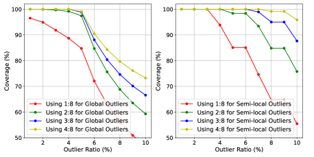
Figure 5: Local outlier extraction using N:8 for global outliers and semi-local outliers.

To demonstrate this, in the left plot of the Figure 5, how much coverage N:8 local outlier extraction show on one of the OPT-6.7B layer. As expected, we observe that 2:8 is enough capture 99% of global outliers if the outlier ratio is smaller than 4%.

Moreover, N:M local outlier extraction would be more efficient with the recent trend of finer granularity for the scale factors, i.e. smaller Q-Vector size. As a separate scale factor would be used for each Q-Vector, the outlier extraction needs to capture semi-local (Q-Vector-wise) outliers, not the global outliers.

In the right plot of the  Figure 5, we show how N:M local outlier extraction is able to cover semi-local outliers when the Q-Vector size is 64. As expected, N:M local outlier extraction is able to show much higher coverage for semi-local outliers than global outliers, for example, 1:8 is enough to capture all semi-local outliers up to 3% outlier ratio, thanks to its relatively regular outlier pattern.

5 SDQ For LLMs

In this section, we explain our framework for SDQ. As the name implies, it consists of three stages, sparsificaion, decomposition, and quantization, where each stage can leverage different existing methods and works together as a hybrid method.

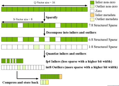
Figure 6: SDQ flow with a vector size of 16.

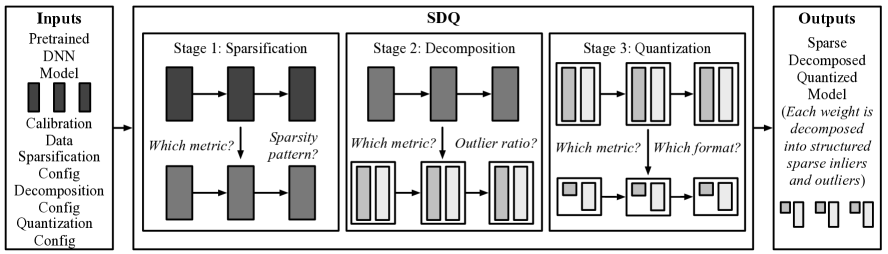
Figure 7: Overall SDQ framework composed of three stages.

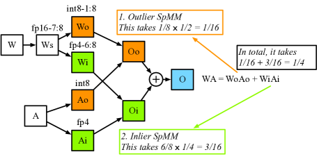
Figure 8: Performance estimation with SDQ.

Stage 1 Sparsification: SDQ first sparsify the weights of LLMs as much as possible, until the LLM quality are impacted signicantly (e.g., 1% increase in perplexity). SDQ prunes weights based on a significance metric under the structured pattern constraint, such as N:M. The most straightforward metric is magnitude as the weight with a small magnitude is likely to not affect much to the final output Mishra et al. (2021). The framework only keeps the largest N values in each block that is composed of consecutive M values.

If using calibration data is allowed, more sophisticated metrics could be used. For example, another metric is based on weight-activation-product (Wanda Sun et al. (2023)) that is able to take the activation into account while choosing the significant weight values. Even though a weight value itself is tiny, it is possible that the corresponding activation is huge, increasing the impact to the output. We also use SparseGPT Frantar & Alistarh (2023) that is also using calibration data. Unlike the previous methods, SparseGPT updates weights in the sparsification to compensate for the error during the process and uses a Hessian-based metric as a significance metric. In Figure 6, the sparsification stage uses 6:8 as the target structured sparsity using the given significance metric.

	OPT
Optimization Configuration	125M	350M	1.3B	2.7B	6.7B	13B	30B
1$\times$ Effective Compute Throughput
Dense-WA16	27.65	22.00	14.62	12.47	10.86	10.13	9.56
S-RTN-W4	-	-	-	-	12.10	11.32	10.97
S-GPTQ-W4	-	-	-	-	11.39	10.31	9.63
S-SpQR-W4	-	-	-	-	11.04	10.28	9.54
2$\times$ Effective Compute Throughput
S-Wanda-4:8	53.12	58.90	22.21	16.77	13.55	13.35	10.87
S-SparseGPT-4:8	43.99	38.92	20.06	15.04	12.57	11.83	10.31
Q-VSQuant-WAint8	27.77	22.01	14.75	12.50	10.95	10.14	9.57
Q-VSQuant-WAffp8	27.78	22.05	14.75	12.51	10.95	10.13	9.58
3.6$\times$ Effective Compute Throughput
SDQ-8:8-1:8int8-7:8fp4	28.99	22.87	15.36	12.62	11.06	10.24	9.66
4$\times$ Effective Compute Throughput
S-Wanda-2:8	1584.81	2847.39	1217.73	6204.19	1028.50	2010.05	9997.60
S-SparseGPT-2:8	849.99	645.33	990.81	150.09	189.00	265.05	97.92
Q-VSQuant-WAint4	33.10	28.25	17.84	14.63	12.02	11.72	10.61
Q-VSQuant-WAfp4	30.50	24.31	16.00	13.29	11.32	10.57	9.90
SDQ-W3:4-1:4int8-2:4fp4	31.42	26.76	16.33	13.11	11.17	10.41	9.63
SDQ-S3:4-1:4int8-2:4fp4	30.71	25.84	16.35	12.96	11.15	10.31	9.58
SDQ-W6:8-2:8int8-4:8fp4	30.15	24.48	15.71	12.68	10.91	10.27	9.51
SDQ-S6:8-2:8int8-4:8fp4	29.70	24.45	16.41	12.58	10.98	10.20	9.52
SDQ-W7:8-1:8int8-6:8fp4	29.30	23.02	15.44	12.70	10.89	10.21	9.58
SDQ-S7:8-1:8int8-6:8fp4	28.82	23.20	15.83	12.56	10.98	10.26	9.60

Table 2: Perplexity results of OPT on raw-WikiText2 with various sparsification, quantization, and SDQ configurations.

Stage 2 Decomposition: In this stage, SDQ decomposes the the weight tensor of each layer into two tensors, inliers and outliers using the N:M local outlier extraction explained in section 4. In Figure 6, it uses 1:8 as the target structured sparsity for the local outlier extraction so that the remaining values become the inliers. An interesting point in this example after extracting outliers as 1:8 is that the remaining outlier becomes naturally structured sparse, in this case, 6:8.

To choose outliers, we need another metric to decide whether a weight value is an outlier or not, similar to the significance metric for sparsification. We experiment with magnitude-based, activation-weight-product-based, and output-error-based metrics (based on the error after quantization). Unlike previous work, we make sure both inlier and outlier tensors are N:M structured sparse so that we can utilize efficient SpMM on structured sparse HW.

Stage 3 Quantization: The last stage of SDQ is quantization where it uses different number formats for structured sparse inliers and outliers. For quantization, we use VS-Quant Dai et al. (2021) as it provides flexibility in the granularity of scale factors. We use a relatively higher bit width for outliers while using a lower bit width for inliers. We also quantize activations accordingly so that we can use low-bit arithmetic computations that are cheaper in terms of area and power. We show the high-level overview of the SDQ framework in Figure 7.

5.1 LLM inference performance

In Figure 8, we show how SDQ unveils 4$\times$ compute throughput. As explained, the weights, $W$, is sparsified to $W_{s}$, then decomposed to $W_{o}$ and $W_{i}$. We quantize 1:8 $W_{o}$ as int8 and 6:8 $W_{i}$ as fp4; accordingly, activation $A$ would be quantized to int8 $A_{o}$ and fp4 $A_{i}$. Then, output activation from outliers $O_{o}$ is calculated through SpMM, which takes $\frac{1}{8}\times\frac{1}{2}=\frac{1}{16}$ using 1:8 and 8 bit computations compared to fp16 baseline. Similarly, output activation from inliers $O_{i}$ is computed through SpMM, which takes $\frac{6}{8}\times\frac{1}{4}=\frac{3}{16}$ using 6:8 and fp4 computations compared to fp16 baseline. Thus, in total, it takes $\frac{1}{16}+\frac{3}{16}=\frac{1}{4}$, thus providing $4\times$ effective compute throughput. The achieved effective compute throughput would depend on the target structured sparsity and number format, so we explore different configurations in section 6.

6 Evaluation

	LLaMA-1			LLaMA-2
Optimization Configuration	7B	13B	30B	7B	13B
1$\times$ Effective Compute Throughput
Baseline	5.68	5.09	4.10	5.12	4.57
S-RTN-W4	6.43	5.55	4.57	-	-
S-GPTQ-W4	6.13	5.40	4.48	-	-
S-SpQR-W4	5.87	5.22	4.25	-	-
2$\times$ Effective Compute Throughput
S-Wanda-4:8	8.57	7.41	5.97	8.07	6.55
S-SparseGPT-4:8	8.61	7.42	6.15	7.91	6.58
Q-VSQuant-WA-int8	5.70	5.11	4.13	5.14	4.60
Q-VSQuant-WA-fp8	5.70	5.11	4.12	5.14	4.59
3.6$\times$ Effective Compute Throughput
SDQ-8:8-1:8int8-7:8fp4	5.81	5.20	4.22	5.23	4.67
4$\times$ Effective Compute Throughput
S-Wanda-2:8	2960.99	2481.10	1228.86	1947.60	1188.45
S-SparseGPT-2:8	151.93	96.30	58.67	75.99	85.99
Q-VSQuant-WA-int4	6.48	5.91	4.76	6.85	5.33
Q-VSQuant-WA-fp4	5.97	5.29	4.33	5.36	4.74
SDQ-W3:4-1:4int8-2:4fp4	6.30	5.53	4.60	5.67	5.00
SDQ-S3:4-1:4int8-2:4fp4	6.30	5.54	4.67	5.65	4.98
SDQ-W6:8-2:8int8-4:8fp4	6.10	5.37	4.45	5.48	4.87
SDQ-S6:8-2:8int8-4:8fp4	6.10	5.36	4.50	5.48	4.86
SDQ-W7:8-1:8int8-6:8fp4	5.87	5.25	4.27	5.30	4.73
SDQ-S7:8-1:8int8-6:8fp4	5.88	5.26	4.31	5.32	4.73

Table 3: Perplexity results of LLaMA-1/LLaMA-2 on raw-WikiText2 with various sparsification, quantization, and SDQ configurations.

6.1 Methodology

In this section, we show how our hybrid method, SDQ, can be applied to LLMs to push the limit of effective compute throughput while achieving higher model quality than sparsification-only or quantization-only method. We use OPT Zhang et al. (2022), LLaMA Touvron et al. (2023a), LLaMA-2 Touvron et al. (2023b) with different number of parameters, from 125M to 30B. We use the fp16 dense version of each model as the baseline model.

First, we measure the perplexity change on the raw-Wikitext2 with OPT/LLaMA-1/LLaMA-2 from 125M to 30B parameters using various SDQ configurations. Next, we provide zero-shot evaluation results of SDQ on OPT-6.7B, LLaMA-1-7B, and LLaMA-2-7B with BoolQ, HellaSwag, WinoGrande, ARC-e, ARC-c, and PIQA from LM-Eval Gao et al. (2021). For baseline sparsification-only and quantization-only methods, we use SparseGPT Frantar & Alistarh (2023), Wanda Sun et al. (2023), and VS-Quant Dai et al. (2021) with Q-Vector size of 16. Only for the weight-only quantization methods (S-RTN-W4, S-GPTQ-W4, S-SpQR-W4), we use the results reported in the publication Dettmers et al. (2023).

We also compare different SDQ configurations. For example, SDQ-W7:8-1:8int8-6:8fp4 means 1) using Wanda (we use S for SparseGPT) as sparsification with 7:8 structured sparsity 2) and using 1:8 local outlier extraction with int8 and 6:8 inlier with fp4. For decomposition metric, we find the product-based one Sun et al. (2023) performs the best, so we use the metric. Starting with S- indicates sparsification-only and Q- indicates quantization-only (WA means dual quantization and W means weight-only).

6.2 Perplexity evaluation

We summarize the result of perplexity evaluation in Table 2 for various OPT models.

Comparison against sparsification. As mentioned in  section 4, sparsification-only methods are not effective both for $2\times$ and $4\times$ effective compute throughput categories. For 2$\times$ category, S-SparseGPT-4:8 gives the best perplexity, increasing 8% compared to the baseline model perplexity. Considering 1% quality loss as the criteria, this is not acceptable; for instance, using baseline OPT-1.3B would be much better than using 4:8 OPT-2.7B, showing no benefits of using sparsification-only methods. This gets even worse for small models. For example, we found OPT-125M with the same configuration cause 59% increase in terms of perplexity. For 4$\times$ throughput category, the model gets totally broken with sparsification-only methods due to the not enough number of elements that the model can keep.

Comparison against weight-only quantization. We observe that SDQ can achieve better perplexity than the best weight-only 4b quantization (fp4-e2m1) while enabling 4$\times$ effective compute throughput. For example, OPT-30B with SDQ-W6:8-2:8o8b-4:8i4b results in the perplexity of 9.51 which is better than that of S-SpQR-W4 (9.54) or even Dense-WA16 baseline (9.56).

OPT-6.7B
Method	BoolQ	HellaSwag	WinoGrande	ARC-easy	ARC-challenge	PIQA	Average
Baseline	66.15	50.53	65.19	65.61	30.55	76.22	59.04
S-SparseGPT-2:8	58.50	27.63	51.22	32.11	19.45	56.20	40.85
S-Wanda-2:8	50.03	26.22	50.36	31.02	18.69	55.33	38.61
Q-VSQuant-WA-int4	61.38	47.09	60.85	59.64	26.88	71.27	54.52
Q-VSQuant-WA-fp4	62.94	48.50	61.80	65.15	29.18	74.70	57.05
SDQ-7:8-1:8int8-6:8fp4	66.33	49.91	63.54	65.23	30.20	74.97	58.36
LLaMA-1-7B
Baseline	75.11	56.95	69.85	75.29	41.89	78.67	66.29
S-SparseGPT-2:8	45.02	27.93	48.54	31.02	18.34	54.79	37.61
S-Wanda-2:8	37.83	26.35	50.04	26.52	20.65	53.43	35.80
Q-VSQuant-WA-int4	73.91	54.42	67.88	72.56	37.88	77.15	63.97
Q-VSQuant-WA-fp4	74.86	56.06	69.38	74.54	40.87	77.26	65.49
SDQ-7:8-1:8int8-6:8fp4	75.35	56.24	69.30	74.70	41.38	78.29	65.88
LLaMA-2-7B
Baseline	77.74	57.13	69.06	76.30	43.43	78.07	66.96
S-SparseGPT-2:8	48.10	27.92	45.38	28.62	17.58	54.90	37.08
S-Wanda-2:8	37.83	26.15	50.91	26.94	19.62	52.82	35.71
Q-VSQuant-WA-int4	74.62	53.51	66.85	72.90	40.27	76.38	64.09
Q-VSQuant-WA-fp4	75.81	55.99	67.96	75.17	41.38	77.26	65.60
SDQ-7:8-1:8int8-6:8fp4	78.44	56.43	67.09	76.13	43.17	77.58	66.47

Table 4: Zero-shot evaluation on various tasks with OPT-6.7B, LLaMA-1-7B, and LLaMA-2-7B.

Comparison against dual quantization. Using dual quantization, one can achieve 2$\times$ and 4$\times$ if both weights and activations are quantized to 8-bit and 4-bit, respectively. For the 2$\times$ category, quantizing weights and activation with INT8 (or FP8) did not hurt the model quality, which is consistent to what the previous work Dettmers et al. (2022) found. For the 4$\times$ category, quantizing weights and activation with INT4 causes 9.9%$-$19.7% perplexity increases while that with FP4 causes 3.6%$-$10.3% perplexity increases, which is still significant quality loss based on the 1% criteria. Using SDQ, we observe that SDQ cause 0%$-$4.2% perplexity increaeses depending on the model sizes, which is significantly smaller than other 4$\times$ methods. For the larger model, such as 2.7B, 6.7B, and 13B, we observe SDQ incurs less than 1% perplexity increase, and interestingly, for OPT-30B, SDQ is able to reduce the perplexity, enabling 4$\times$ effective compute throughput with less than 1% model quality drop.

We find the overall similar trend for LLaMA-1 and LLaMA-2 models as reported in Table 3.

6.3 Zero-shot evaluation

To provide a more holistic evaluation, we conduct experiments on various Zero-shot tasks and show the results in  Table 4. These are known to provide more noisy results Dettmers et al. (2022), but still provide a big picture in terms of applicability. As the individual result for each task could be noisy, we compare the average accuracy of all the zero-shot tasks. To achieve 4$\times$ effective compute throughput, we observe the best sparsification-only and quantization-only methods show 25.58% and 1.37% accuracy drop, respectively, while SDQ only causes 0.53% accuracy drop, showing the similar trend that we observe in the perplexity evaluation. SDQ is the only option that meets the 1% criteria.

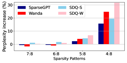
Figure 9: Sensitivity study with different sparsification methods

6.4 Sensitivity studies

SDQ is composed of the three stages and the performance of the effectiveness of SDQ is also affected by the effectiveness of each stage. We use OPT-6.7B for this study.

Sparsification stage. In Figure 9, we show how different sparsity patterns and sparsification method affects to the effectiveness of SDQ. First, we observe that Wanda performs better than SparseGPT for 7:8 and 6:8 (even exceeding the baseline) while SparseGPT performs better than Wanda for 5:8 and 4:8. Next, we apply SDQ with SparseGPT and Wanda for the sparsification stage with $N$:8 where $N$ is 7, 6, 5, and 4. We use 1:8 int8 for outliers, and $N$-1:8 for inliers for each $N$ (as we use the same decomposition and quantization configuration for all SDQ options in this experiment, we just call them as SDQ-S and SDQ-W). We observe the same trend for SDQ-S and SDQ-W, similar to the sparsification-only methods; for 7:8/6:8, SDQ-W exhibits lower (better) perplexity than SDQ-S while SDQ-S exhibits lower (better) perplexity than SDQ-W for 5:8/4:8.

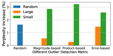
Figure 10: Sensitivity study with different decomposition metrics.

Decomposition stage. In Figure 10, we show how different decomposition method affects to the effectiveness of SDQ. We use SDQ-W7:8-1:8int8-6:8fp4, but with different criteria in the decomposition stage. In the decomposition stage, a metric is required for N:M local outlier extraction to identify the outliers. The simplest one is using the magnitude Guo et al. (2023), but more sophisticated metrics could also be used such as weight-activation-product-based used in Wanda Sun et al. (2023) or error-based similar to the one used in SpQR Dettmers et al. (2023). Also, we can determine an element as an outlier based on the ascending or descending order of the metric. We mark “Large” in the plot if we select outliers in descending order, and “Small” if we select in ascending order. We observe that product-based outlier extraction performs the best and the perplexity could fluctuate up to 7% depending on the extracted outliers, implying that adopting an effective method to extract outliers is critical for the effectiveness of SDQ. We leave exploring the best method to locate outliers for future work.

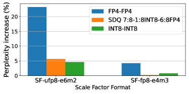
Figure 11: Sensitivity study with different scale factor formats.

Quantization stage. VS-Quant can use different number formats for scale factor per Q-Vector. In Figure 11, we show how different quantization configurations, such as the scale factor format, affect the effectiveness of SDQ. We compare two formats: ufp8-e6m2 (unsigned float using 6 bits for exponents and 2 bits for mantissa) and fp8-e4m3 (signed float using 4 bits for exponents and 3 bits for mantissa and 1 bit as the sign bit). We observe that dual quantization using fp4 with ufp8-e6m2 scale factors performs much worse than the case with fp8-e4m3. Similarly, dual quantization with int8 also prefers fp8-e4m3 scale factors than ufp8-e6m2. We also observe that SDQ-W7:8-1:8int8-6:8fp4 prefers fp8-e4m3, showing that improving quantization could also improve the quality of SDQ.

7 Related Work

Both SparseGPT Frantar & Alistarh (2023) and Wanda Sun et al. (2023) propose sparsification methods for LLMs, but they both fail to maintain the quality of the model even with 50% N:M sparsity (such as 2:4 or 4:8). Unlike sparsification, there have been many attempts to quantize LLMs Frantar et al. (2023); Lin et al. (2023); Dettmers et al. (2023; 2022); Xiao et al. (2023); Kim et al. (2023). We use VS-Quant Dai et al. (2021) in the current SDQ, but our work is not limited to the quantization method as shown in subsection 6.4. We believe SDQ can take the benefits of the improvement in quantization methods.

OBC Frantar et al. (2022) provides a framework for quantization and sparsification, but they do not target LLMs. Also, they do not consider running LLMs efficiently through N:M structured sparse HW and low-bit computations. Recent work Kuzmin et al. (2023) observe that quantization generally performs better than sparsification on Vision models, which is consistent with our observation for LLMs.

8 Conclusion

We propose a new method, Sparse Decomposed Quantization (SDQ) using mixed precision for outliers and inliers through structured decomposition, which enables utilizing mixed precision N:M structured sparse HW. We explore the SDQ across different models and sizes to understand the potential of the technique with various LLMs. We show that SDQ opens up an opportunity to achieve 4$\times$ effective compute throughput while maintaining the model quality ($<1\%$ quality drop). We plan to extend this to validate with sparse tensor accelerator simulators, such as Sparseloop Wu et al. (2022).

References

- Brown et al. (2020) Brown, T. B., Mann, B., Ryder, N., Subbiah, M., Kaplan, J., Dhariwal, P., Neelakantan, A., Shyam, P., Sastry, G., Askell, A., Agarwal, S., Herbert-Voss, A., Krueger, G., Henighan, T., Child, R., Ramesh, A., Ziegler, D. M., Wu, J., Winter, C., Hesse, C., Chen, M., Sigler, E., Litwin, M., Gray, S., Chess, B., Clark, J., Berner, C., McCandlish, S., Radford, A., Sutskever, I., and Amodei, D. Language models are few-shot learners, 2020.
- Chowdhery et al. (2022) Chowdhery, A., Narang, S., Devlin, J., Bosma, M., Mishra, G., Roberts, A., Barham, P., Chung, H. W., Sutton, C., Gehrmann, S., Schuh, P., Shi, K., Tsvyashchenko, S., Maynez, J., Rao, A., Barnes, P., Tay, Y., Shazeer, N., Prabhakaran, V., Reif, E., Du, N., Hutchinson, B., Pope, R., Bradbury, J., Austin, J., Isard, M., Gur-Ari, G., Yin, P., Duke, T., Levskaya, A., Ghemawat, S., Dev, S., Michalewski, H., Garcia, X., Misra, V., Robinson, K., Fedus, L., Zhou, D., Ippolito, D., Luan, D., Lim, H., Zoph, B., Spiridonov, A., Sepassi, R., Dohan, D., Agrawal, S., Omernick, M., Dai, A. M., Pillai, T. S., Pellat, M., Lewkowycz, A., Moreira, E., Child, R., Polozov, O., Lee, K., Zhou, Z., Wang, X., Saeta, B., Diaz, M., Firat, O., Catasta, M., Wei, J., Meier-Hellstern, K., Eck, D., Dean, J., Petrov, S., and Fiedel, N. Palm: Scaling language modeling with pathways, 2022.
- Dai et al. (2021) Dai, S., Venkatesan, R., Ren, M., Zimmer, B., Dally, W., and Khailany, B. Vs-quant: Per-vector scaled quantization for accurate low-precision neural network inference. Proceedings of Machine Learning and Systems, 3:873–884, 2021.
- Darvish Rouhani et al. (2023) Darvish Rouhani, B., Zhao, R., Elango, V., Shafipour, R., Hall, M., Mesmakhosroshahi, M., More, A., Melnick, L., Golub, M., Varatkar, G., Shao, L., Kolhe, G., Melts, D., Klar, J., L’Heureux, R., Perry, M., Burger, D., Chung, E., Deng, Z. S., Naghshineh, S., Park, J., and Naumov, M. With shared microexponents, a little shifting goes a long way. In Proceedings of the 50th Annual International Symposium on Computer Architecture, ISCA ’23, New York, NY, USA, 2023. Association for Computing Machinery. ISBN 9798400700958. doi: 10.1145/3579371.3589351. URL https://doi.org/10.1145/3579371.3589351.
- Dettmers et al. (2022) Dettmers, T., Lewis, M., Belkada, Y., and Zettlemoyer, L. Llm.int8(): 8-bit matrix multiplication for transformers at scale. In Koyejo, S., Mohamed, S., Agarwal, A., Belgrave, D., Cho, K., and Oh, A. (eds.), Advances in Neural Information Processing Systems, volume 35, pp. 30318–30332. Curran Associates, Inc., 2022.
- Dettmers et al. (2023) Dettmers, T., Svirschevski, R., Egiazarian, V., Kuznedelev, D., Frantar, E., Ashkboos, S., Borzunov, A., Hoefler, T., and Alistarh, D. Spqr: A sparse-quantized representation for near-lossless llm weight compression, 2023.
- Frantar & Alistarh (2023) Frantar, E. and Alistarh, D. SparseGPT: Massive language models can be accurately pruned in one-shot. arXiv preprint arXiv:2301.00774, 2023.
- Frantar et al. (2022) Frantar, E., Singh, S. P., and Alistarh, D. Optimal Brain Compression: a framework for accurate post-training quantization and pruning. Advances in Neural Information Processing Systems, 36, 2022.
- Frantar et al. (2023) Frantar, E., Ashkboos, S., Hoefler, T., and Alistarh, D. OPTQ: Accurate quantization for generative pre-trained transformers. In The Eleventh International Conference on Learning Representations, 2023. URL https://openreview.net/forum?id=tcbBPnfwxS.
- Gao et al. (2021) Gao, L., Tow, J., Biderman, S., Black, S., DiPofi, A., Foster, C., Golding, L., Hsu, J., McDonell, K., Muennighoff, N., Phang, J., Reynolds, L., Tang, E., Thite, A., Wang, B., Wang, K., and Zou, A. A framework for few-shot language model evaluation, September 2021. URL https://doi.org/10.5281/zenodo.5371628.
- Guo et al. (2023) Guo, C., Tang, J., Hu, W., Leng, J., Zhang, C., Yang, F., Liu, Y., Guo, M., and Zhu, Y. Olive: Accelerating large language models via hardware-friendly outlier-victim pair quantization. In Proceedings of the 50th Annual International Symposium on Computer Architecture, ISCA ’23, New York, NY, USA, 2023. Association for Computing Machinery. ISBN 9798400700958. doi: 10.1145/3579371.3589038. URL https://doi.org/10.1145/3579371.3589038.
- Han et al. (2015) Han, S., Pool, J., Tran, J., and Dally, W. Learning both weights and connections for efficient neural network. In Cortes, C., Lawrence, N., Lee, D., Sugiyama, M., and Garnett, R. (eds.), Advances in Neural Information Processing Systems, volume 28. Curran Associates, Inc., 2015. URL https://proceedings.neurips.cc/paper_files/paper/2015/file/ae0eb3eed39d2bcef4622b2499a05fe6-Paper.pdf.
- Hoefler et al. (2021) Hoefler, T., Alistarh, D., Ben-Nun, T., Dryden, N., and Peste, A. Sparsity in deep learning: Pruning and growth for efficient inference and training in neural networks. J. Mach. Learn. Res., 22(1), jan 2021. ISSN 1532-4435.
- Horowitz (2014) Horowitz, M. 1.1 computing’s energy problem (and what we can do about it). In 2014 IEEE International Solid-State Circuits Conference Digest of Technical Papers (ISSCC), pp. 10–14, 2014. doi: 10.1109/ISSCC.2014.6757323.
- Jeong et al. (2023) Jeong, G., Damani, S., Bambhaniya, A. R., Qin, E., Hughes, C. J., Subramoney, S., Kim, H., and Krishna, T. Vegeta: Vertically-integrated extensions for sparse/dense gemm tile acceleration on cpus. In 2023 IEEE International Symposium on High Performance Computer Architecture (HPCA), 2023.
- Kim et al. (2023) Kim, S., Hooper, C., Gholami, A., Dong, Z., Li, X., Shen, S., Mahoney, M., and Keutzer, K. Squeezellm: Dense-and-sparse quantization. arXiv, 2023.
- Kuzmin et al. (2023) Kuzmin, A., Nagel, M., van Baalen, M., Behboodi, A., and Blankevoort, T. Pruning vs quantization: Which is better?, 2023.
- LeCun et al. (1989) LeCun, Y., Denker, J., and Solla, S. Optimal brain damage. In Touretzky, D. (ed.), Advances in Neural Information Processing Systems, volume 2. Morgan-Kaufmann, 1989. URL https://proceedings.neurips.cc/paper_files/paper/1989/file/6c9882bbac1c7093bd25041881277658-Paper.pdf.
- Lee et al. (2023) Lee, C., Jin, J., Kim, T., Kim, H., and Park, E. Owq: Lessons learned from activation outliers for weight quantization in large language models. arXiv preprint arXiv:2306.02272, 2023.
- Lin et al. (2023) Lin, J., Tang, J., Tang, H., Yang, S., Dang, X., Gan, C., and Han, S. Awq: Activation-aware weight quantization for llm compression and acceleration, 2023.
- Liu et al. (2021) Liu, Z.-G., Whatmough, P. N., Zhu, Y., and Mattina, M. S2ta: Exploiting structured sparsity for energy-efficient mobile cnn acceleration. arXiv preprint arXiv:2107.07983, 2021.
- Micikevicius (2021) Micikevicius, P. Sparsity, structure, and performance, 2021. Sparsity in Neural Networks (SNN) Workshop.
- Mishra et al. (2021) Mishra, A., Latorre, J. A., Pool, J., Stosic, D., Stosic, D., Venkatesh, G., Yu, C., and Micikevicius, P. Accelerating sparse deep neural networks. arXiv preprint arXiv:2104.08378, 2021.
- Molchanov et al. (2022) Molchanov, P., Hall, J., Yin, H., Kautz, J., Fusi, N., and Vahdat, A. Lana: latency aware network acceleration. In European Conference on Computer Vision, pp. 137–156. Springer, 2022.
- NVIDIA (2020) NVIDIA. Nvidia ampere ga102 gpu architecture, 2020. https://www.nvidia.com/content/PDF/nvidia-ampere-ga-102-gpu-architecture-whitepaper-v2.1.pdf.
- NVIDIA (2022) NVIDIA. Nvidia h100 tensor core gpu architecture, 2022. https://resources.nvidia.com/en-us-tensor-core.
- Pool et al. (2021) Pool, J., Sawarkar, A., and Rodge, J. Accelerating inference with sparsity using the nvidia ampere architecture and nvidia tensorrt, 2021. URL https://developer.nvidia.com/blog/accelerating-inference-with-sparsity-using-ampere-and-tensorrt/.
- Qin et al. (2020) Qin, E., Samajdar, A., Kwon, H., Nadella, V., Srinivasan, S., Das, D., Kaul, B., and Krishna, T. Sigma: A sparse and irregular gemm accelerator with flexible interconnects for dnn training. In 2020 IEEE International Symposium on High Performance Computer Architecture (HPCA), pp. 58–70, 2020. doi: 10.1109/HPCA47549.2020.00015.
- Reddi et al. (2020) Reddi, V. J., Cheng, C., Kanter, D., Mattson, P., Schmuelling, G., Wu, C.-J., Anderson, B., Breughe, M., Charlebois, M., Chou, W., Chukka, R., Coleman, C., Davis, S., Deng, P., Diamos, G., Duke, J., Fick, D., Gardner, J. S., Hubara, I., Idgunji, S., Jablin, T. B., Jiao, J., John, T. S., Kanwar, P., Lee, D., Liao, J., Lokhmotov, A., Massa, F., Meng, P., Micikevicius, P., Osborne, C., Pekhimenko, G., Rajan, A. T. R., Sequeira, D., Sirasao, A., Sun, F., Tang, H., Thomson, M., Wei, F., Wu, E., Xu, L., Yamada, K., Yu, B., Yuan, G., Zhong, A., Zhang, P., and Zhou, Y. Mlperf inference benchmark. In Proceedings of the ACM/IEEE 47th Annual International Symposium on Computer Architecture, ISCA ’20, pp. 446–459. IEEE Press, 2020. ISBN 9781728146614. doi: 10.1109/ISCA45697.2020.00045. URL https://doi.org/10.1109/ISCA45697.2020.00045.
- Sun et al. (2023) Sun, M., Liu, Z., Bair, A., and Kolter, J. Z. A simple and effective pruning approach for large language models. arXiv preprint arXiv:2306.11695, 2023.
- Touvron et al. (2023a) Touvron, H., Lavril, T., Izacard, G., Martinet, X., Lachaux, M.-A., Lacroix, T., Rozière, B., Goyal, N., Hambro, E., Azhar, F., Rodriguez, A., Joulin, A., Grave, E., and Lample, G. Llama: Open and efficient foundation language models, 2023a.
- Touvron et al. (2023b) Touvron, H., Martin, L., Stone, K., Albert, P., Almahairi, A., Babaei, Y., Bashlykov, N., Batra, S., Bhargava, P., Bhosale, S., Bikel, D., Blecher, L., Ferrer, C. C., Chen, M., Cucurull, G., Esiobu, D., Fernandes, J., Fu, J., Fu, W., Fuller, B., Gao, C., Goswami, V., Goyal, N., Hartshorn, A., Hosseini, S., Hou, R., Inan, H., Kardas, M., Kerkez, V., Khabsa, M., Kloumann, I., Korenev, A., Koura, P. S., Lachaux, M.-A., Lavril, T., Lee, J., Liskovich, D., Lu, Y., Mao, Y., Martinet, X., Mihaylov, T., Mishra, P., Molybog, I., Nie, Y., Poulton, A., Reizenstein, J., Rungta, R., Saladi, K., Schelten, A., Silva, R., Smith, E. M., Subramanian, R., Tan, X. E., Tang, B., Taylor, R., Williams, A., Kuan, J. X., Xu, P., Yan, Z., Zarov, I., Zhang, Y., Fan, A., Kambadur, M., Narang, S., Rodriguez, A., Stojnic, R., Edunov, S., and Scialom, T. Llama 2: Open foundation and fine-tuned chat models, 2023b.
- van Baalen et al. (2023) van Baalen, M., Kuzmin, A., Nair, S. S., Ren, Y., Mahurin, E., Patel, C., Subramanian, S., Lee, S., Nagel, M., Soriaga, J., and Blankevoort, T. Fp8 versus int8 for efficient deep learning inference, 2023.
- Vaswani et al. (2017) Vaswani, A., Shazeer, N., Parmar, N., Uszkoreit, J., Jones, L., Gomez, A. N., Kaiser, L. u., and Polosukhin, I. Attention is all you need. In Guyon, I., Luxburg, U. V., Bengio, S., Wallach, H., Fergus, R., Vishwanathan, S., and Garnett, R. (eds.), Advances in Neural Information Processing Systems, volume 30. Curran Associates, Inc., 2017. URL https://proceedings.neurips.cc/paper_files/paper/2017/file/3f5ee243547dee91fbd053c1c4a845aa-Paper.pdf.
- Wu et al. (2022) Wu, Y. N., Tsai, P.-A., Parashar, A., Sze, V., and Emer, J. S. Sparseloop: An analytical approach to sparse tensor accelerator modeling. In 2022 55th IEEE/ACM International Symposium on Microarchitecture (MICRO), pp. 1377–1395, 2022. doi: 10.1109/MICRO56248.2022.00096.
- Wu et al. (2023) Wu, Y. N., Tsai, P.-A., Muralidharan, S., Parashar, A., Sze, V., and Emer, J. S. Highlight: Efficient and flexible dnn acceleration with hierarchical structured sparsity. In 2023 56th IEEE/ACM International Symposium on Microarchitecture (MICRO), 2023.
- Xiao et al. (2023) Xiao, G., Lin, J., Seznec, M., Wu, H., Demouth, J., and Han, S. SmoothQuant: Accurate and efficient post-training quantization for large language models. In Proceedings of the 40th International Conference on Machine Learning, 2023.
- Yin et al. (2023) Yin, L., Wu, Y., Zhang, Z., Hsieh, C.-Y., Wang, Y., Jia, Y., Pechenizkiy, M., Liang, Y., Wang, Z., and Liu, S. Outlier weighed layerwise sparsity (owl): A missing secret sauce for pruning llms to high sparsity. arXiv preprint arXiv:2310.05175, 2023.
- Zhang et al. (2022) Zhang, S., Roller, S., Goyal, N., Artetxe, M., Chen, M., Chen, S., Dewan, C., Diab, M., Li, X., Lin, X. V., Mihaylov, T., Ott, M., Shleifer, S., Shuster, K., Simig, D., Koura, P. S., Sridhar, A., Wang, T., and Zettlemoyer, L. Opt: Open pre-trained transformer language models, 2022.
- Zhu et al. (2019) Zhu, M., Zhang, T., Gu, Z., and Xie, Y. Sparse tensor core: Algorithm and hardware co-design for vector-wise sparse neural networks on modern gpus. In Proceedings of the 52nd Annual IEEE/ACM International Symposium on Microarchitecture, MICRO ’52, pp. 359–371, New York, NY, USA, 2019. Association for Computing Machinery. ISBN 9781450369381.