Error-Correcting Graph Codes

Abstract

In this paper, we define, study, and construct Error-Correcting Graph Codes. An error-correcting graph code of distance $\delta$ is a family $C$ of graphs, on a common vertex set of size $n$, such that if we start with any graph in $C$, we would have to modify the neighborhoods of at least $\delta n$ vertices in order to reach some other graph in $C$.

This is a natural graph generalization of the standard Hamming distance error-correcting codes for binary strings. We show:

1. Combinatorial results determining the optimal rate vs distance tradeoff nonconstructively.

2. A connection to rank-metric codes, enabling some simple and some involved constructions achieving certain positive rates and distances.

3. Graph code analogues of Reed-Solomon codes and code concatenation, leading to positive distance codes for all rates and positive rate codes for all distances.

4. Graph code analogues of dual-BCH codes, yielding large codes with distance $\delta=1-o(1)$. This gives an explicit “graph code of Ramsey graphs”.

Several recent works, starting with the paper of Alon, Gujgiczer, Körner, Milojević, and Simonyi, have studied more general graph codes; where the symmetric difference between any two graphs in the code is required to have a desired property. Error-correcting graph codes are a particularly interesting instantiation of this concept.

1 Introduction

In this paper, we define, study, and construct Error-Correcting Graph Codes. These are large families of graphs on the same vertex set such that any two graphs in the family are far apart in a natural graph distance, which we now define.

Informally, the graph distance between two graphs on the same vertex set of size $n$ measures the minimum number of vertices that one needs to delete to make the resulting graphs identical. This can also be thought of as (1) the number of vertices whose neighborhoods one has to modify to go from one graph to another, or (2) the vertex cover number of the symmetric difference of the two graphs, or (3) $n$ minus the largest independent set in the symmetric difference of the two graphs.

Definition: (Graph Distance)  Given two graphs $G$ and $H$ on vertex set $[n]$, the graph distance $\operatorname{d_{graph}}(G,H)$ is the size of the smallest set $S\subseteq[n]$ such that the induced graphs of G and $H$ on vertex set $\overline{S}$ are identical.

This is a very natural metric and encompasses deep information about graphs. For example, note the following two simple facts (1) the graph distance of a graph from the empty graph is $n$ minus the independence number of the graph. (2) the graph distance of a graph from the complete graph is $n$ minus the clique number of the graph. Thus the answer to the question: “how far can a graph be from both the empty graph and the complete graph?” is precisely the question of finding the right bound for the diagonal Ramsey numbers; and the answer is $n-O(\log n)$.

For the more widely studied Hamming metric between graphs (which counts the number of edges that have to be changed to go from one graph to another), error-correcting graph codes in that metric turn out to be equivalent to standard Hamming distance error correcting codes; the graph structure makes no difference to the setting.

Error-correcting graph codes fall into the general framework of graph codes defined by Alon, Gujgiczer, Körner, Milojević, and Simonyi [Alo+23], where for a fixed family $\mathcal{F}$ of graphs, one seeks a large code $C$ of graphs on the same $n$-vertex set such that the symmetric difference of any two graphs in $C$ does not lie in $\mathcal{F}$. This class of problems was studied for a wide variety of natural $\mathcal{F}$ in a number of recent works [Alo+23, Alo23a, Alo23]. As discussed in [Alo23a], for a suitable choice of $\mathcal{F}$, graph codes become equivalent to classical Hamming distance codes. Our instantiation of this framework gives a quite different yet natural notion of error-correction for graphs.

A more general context relevant to error-correcting graph codes is error-correction of strings under more general error patterns. Suppose we have a collection of subsets $S_{i}\subseteq[m]$ for $i\in[t]$, where $\bigcup_{i}S_{i}=[m]$. These $S_{i}$ denote the corruption zones; a single “corruption” of a string $z\in\{0,1\}^{m}$ entails, for some $i\in[t]$, changing $z|_{S_{i}}$ to something arbitrary in $\{0,1\}^{S_{i}}$. We want to design a code $C\subseteq\{0,1\}^{m}$ such that starting at any $x\in C$, if we do fewer than $d$ corruptions to $x$, we do not end up at any $y\in C$ with $y\neq x$. When the $S_{i}$ are all of size $b$ and form a partition of $[m]$ into $t=m/b$ parts, then such a code is exactly the same as a classical Hamming distance code an alphabet of size $2^{b}$. Error-correcting graph codes give a first step into the challenging setting where the $S_{i}$ all pairwise intersect - here we have $m={n\choose 2}$, $t=n$, the $S_{i}$ (which correspond to all edges incident on a given vertex) all have size $n-1$, and every pair $S_{i}$ and $S_{j}$ intersect in exactly $1$ element.

Finally, we note that error-correcting codes are pseudorandom objects, and the connection to Ramsey graphs suggests that error-correcting graph codes might be closely related to pseudorandom graphs. Thus the problem of studying and explicitly constructing pseudorandom family of pseudorandom graphs is interesting in its own right.

1.1 Results

For the graph distance metric between graphs, we develop a theory of error-correcting codes. For a family $C$ of graphs on the vertex set $[n]$, we define the rate $R\in[0,1]$ and the relative distance $\delta$ by:

• $R=\frac{\log_{2}|C|}{{n\choose 2}}$, which measures the size of the code.

• $\delta$ is the largest so that any two graphs in $C$ have graph distance at least $\delta n$.

We will always be interested in asymptotics as $n\to\infty$. Analogous to the classical theory of Hamming distance error-correcting codes on strings, there are combinatorial questions of determining the tradeoff between $R$ and $\delta$, as well as the algorithmic questions of constructing optimal or good such codes explicitly.

Our main results are:

1. We determine the optimal $R$ vs $\delta$ tradeoff; namely:

   $$R=(1-\delta)^{2}-o(1).$$

   In particular, it is possible to have positive constant $\delta$ for all constant $R<1$ and positive constant $R$ for all constant $\delta<1$.

2. We give (strongly) explicit constructions of graph codes which have positive constant $\delta$ for all constant $R<1$. The explicit construction achieves $R=1-O(\delta)$, which is optimal up to the choice of constant in the $O(\delta)$.

3. We give constructions of graph codes which have positive constant $R$ for all constant $\delta<1$. In particular, we give a quasi-polynomial time explicit construction achieving $\delta=1-O(R^{1/4})$, while optimal codes have $\delta=1-R^{1/2}$. We also give an explicit construction with $\delta=1-O(R^{1/6})$, and a strongly explicit construction with $\delta=1-O(R^{1/8})$

4. We give (strongly) explicit constructions of graph codes with very high $\delta=1-O(n^{-\epsilon})$ and nontrivial $R=\Omega(n^{\epsilon-(1/2)})$ for constant $\epsilon>0$. This gives a “graph code of Ramsey graphs” as will be discussed later.

Independent work:

Pat Devlin and Cole Franks [Dev] independently proposed the study of graph error-correcting codes under this metric, determined the optimal $R$ vs $\delta$ tradeoff, and gave some weaker explicit constructions of graph codes that worked for certain ranges of $R$ and $\delta$.

1.2 Techniques

We now discuss our techniques, and in particular, the relationship between rank-metric codes, Hamming distance codes, and graph codes. We will often specify graphs by their adjacency matrices, viewed as matrices with $\mathbb{F}_{2}$ entries.

First we discuss the combinatorial problem of determining the optimal $R$ vs $\delta$ tradeoff. Both our upper and lower bounds are simple adaptations of results from the Hamming distance code setting. An argument similar to the Singleton bound for Hamming distance codes also works in the setting of graph codes; and gives an upper bound on $R$ in terms of $\delta$. For the nonconstructive existence result, we consider a uniformly random $\mathbb{F}_{2}$-linear subspace of the $\mathbb{F}_{2}$-linear space of symmetric $0$-diagonal $n\times n$ matrices (i.e., the space of all adjacency matrices of graphs); this turns out to give a good graph code with the optimal $R$ vs $\delta$ tradeoff.

This existence result tells us that constructions can be $\mathbb{F}_{2}$-linear spaces, and such graph codes can be specified by an $\mathbb{F}_{2}$ basis for it. We say that a construction is explicit if this basis can be produced in $\mathrm{poly}(n)$ time. We say it is strongly explicit if, given $(i,j,k)$, the $(i,j)$ entry of the $k$’th basis element can be computed in $\mathrm{poly}(\log(n))$ time.

We now discuss our explicit and strongly explicit constructions. The main ideas given below are to develop connections to rank-metric codes and Hamming distance codes, and exploit these in various ways.

Rank-metric codes (over $\mathbb{F}_{2}$) are families of $n\times n$ matrices over $\mathbb{F}_{2}$ such that the difference between any two matrices has high rank. These naturally translate into some kind of graph code, as follows. For any $n\times n$ matrix $A$, we can consider the bipartite graph $G$ on $2n$ vertices whose bipartite adjacency matrix is $A$. A simple argument shows that if matrices $A,B$ correspond to bipartite graphs $G,H$, then the graph distance between $G$ and $H$ is at least the rank of $A-B$. Thus the set of all bipartite graphs corresponding to the matrices in a good rank metric code is a good graph code.

There are two fundamental weaknesses in this construction.

1. Any two bipartite graphs with $n$ vertices in each part have graph distance at most $n$. But there are $2n$ vertices – thus this construction is only capable of producing graph codes with $\delta\leq 1/2$.

2. There are only $2^{n^{2}}$ bipartite graphs with $n$ vertices in each part. But these are $2n$ vertex graphs – thus this construction is only capable of producing graph codes with $R\leq 1/2$.

To get explicit codes with $R$ approach $1$ while having positive constant $\delta$ we have two different approaches.

1. The first approach (Symmetric Rank-Metric Codes), which yields an explicit construction but not a strongly explicit construction, is to consider the subcode of a high rate rank-metric code consisting of only valid adjacency matrices (namely symmetric and $0$-diagonal). This turns out to also have quite high rate for simple linear algebra reasons, and the rank distance of the rank-metric code translates into graph distance. This yields the near-optimal $R$ vs $\delta$ tradeoff in the small $\delta$ regime: $R=1-O(\delta)$.

2. The second approach (Fractal Rank-Metric Codes), which yields a strongly explicit construction, but with slightly worse $R$ vs $\delta$ tradeoff in the small $\delta$ regime: $R=1-O(\delta\log\frac{1}{\delta})$. Here we start with the bipartite graph code constructed out of rank-metric codes; in this code half the potential edges are not being used at all. Our idea is to put a smaller bipartite graph code to use these edges. Now one-fourth of all the potential edges are not being used at all, and we repeat with smaller and smaller bipartite graph codes.

To get explicit codes with $\delta$ approaching $1$ while having positive constant $R$, we take a longer detour.

1. First, we give a way to get a good graph code from a classical Hamming-distance linear code $C\subseteq\mathbb{F}_{2}^{n}$. We first consider the tensor code $C\otimes C$, where the elements are matrices all of whose rows and columns are codewords of $C$. These matrices need not be symmetric, nor do they have $0$ diagonal. But interestingly, if we consider the set $C^{*}$ of all matrices in $C\otimes C$ that are symmetric and have $0$ diagonal, then $C^{*}$ is a linear space with quite large dimension. In particular, if the classical Hamming distance code $C$ had positive rate, then so does the graph code $C^{*}$. We call this construction $C^{*}=\mathrm{STCZD}(C)$ (Symmetric Tensor Code with Zero Diagonals).

   It turns out that if $C$ has good relative distance (in the Hamming metric), then $\mathrm{STCZD}(C)$ has good distance in the graph code metric. However the relative graph distance of $\mathrm{STCZD}(C)$ such a code is bounded by the relative distance of $C$ – and since $C$ is a binary code, this can never be more than $1/2$. So, although we saw a new way to construct graph codes from a Hamming distance code, it did not yield the large distance graph code that we desired.

2. Instead, we bring in another idea from the Hamming code world; code concatenation. Instead of constructing a graph code of symmetric zero-diagonal matrices over $\mathbb{F}_{2}$, we instead construct a “large-alphabet graph code” of symmetric zero-diagonal matrices over $\mathbb{F}_{Q}$ for some large $Q=2^{t}$, and then try to reduce the alphabet size down to $2$ by replacing the $Q$-ary symbols with $\mathbb{F}_{2}$-matrices with suitable properties.

   Applying the analogue of $\mathrm{STCZD}$ to a large alphabet code allows one to get large-alphabet graph codes with large $\delta$, approaching $1$ (since over large alphabets Hamming distance codes can have length approaching $1$). Using Reed-Solomon codes as these large alphabet codes also allows us to make the $\mathrm{STCZD}$ construction strongly explicit. Furthermore, when applied to Reed-Solomon codes, these codes have a natural direct description: these are the evaluation tables of low degree bivariate polynomials $P(X,Y)$ on product sets $S\times S$ that are (1) symmetric (to get a symmetric matrix), and (2) multiples of $(X-Y)^{2}$ (to get zero diagonal).

3. What remains now is to develop the right kind of concatenation so that the resulting graph code has good distance. This turns out to be subtle, and requires an “inner code” with a stronger “directed graph distance” property with $\delta$ nearly 1. Fortunately, this inner code we seek is of very slowly growing size, and we may find this by brute force search. This concludes our description of our explicit construction of graph codes with $\delta$ approaching $1$ and positive constant $R$.

Finally, we discuss our constructions for very high distance, $\delta=1-o(1)$. In this regime, as mentioned earlier, this is related to constructions of Ramsey graphs, a difficult problem in pseudorandomness with a long history. Our constructions work up to $\delta=1-\Omega\left(\frac{1}{\sqrt{n}}\right)$; concretely, we get a large linear space of graphs such that all graphs in the family have no clique or independent set of size $\Omega(\sqrt{n})$. The construction is based on polynomials over finite fields of characteristic $2$: When $n=2^{t}$, we consider a linear space of certain low degree univariate polynomials $f(X)$ over $\mathbb{F}_{2^{t}}$, and create the $\mathbb{F}_{2}$ matrix with rows and columns indexed by $\mathbb{F}_{2^{t}}$ whose $x,y$ entry is $\mathsf{Tr}(f(x+y))$. Here $\mathsf{Tr}$ is the finite field trace map from $\mathbb{F}_{2^{t}}$ to $\mathbb{F}_{2}$. The use of $\mathsf{Tr}$ of polynomials is inspired by the construction of dual-BCH codes. We then show that any such matrix has no large clique or independent set unless $\mathsf{Tr}\circ f$ is identically $0$ or identically $1$ (corresponding to the empty and complete graphs respectively). The proof uses the Weil bounds on character sums and a Fourier analytic approach to bound the independence number for the graphs.

Our constructions are listed in table Table 1, and the rate and distance trade offs achieved by them are illustrated in Figure 1.

Name	Approximate Tradeoffs	Strongly Explict?
Bipartite (4.5)	$R=1/2-\delta$	Yes
Symmetrized Gabidulin (4.7)	$R=1-4\delta$	No
Fractal Rank Metric Code (5.1)	$R=1-O(\delta\log(1/\delta))$	Yes
Concatenated RS Tensor Codes (6.10)	$R=(1-\sqrt{\delta})^{4}-o(1)$	No
Double Concatenated RS Tensor Codes	$R=(1-\delta^{1/3})^{6}-o(1)$	No
Triple Concatenated RS Tensor Codes (6.12)	$R=(1-\delta^{1/4})^{8}-o(1)$	Yes
Dual BCH Codes (7.5)	$R=\log(n)(1-\delta)/\sqrt{n}$	Yes

Table 1: A list of constructions of error-correcting graph codes in this paper. All except Concatenated RS Tensor Codes are explicit. Note that the last four constructions are interesting in the regime where $\delta$ is close to $1$.

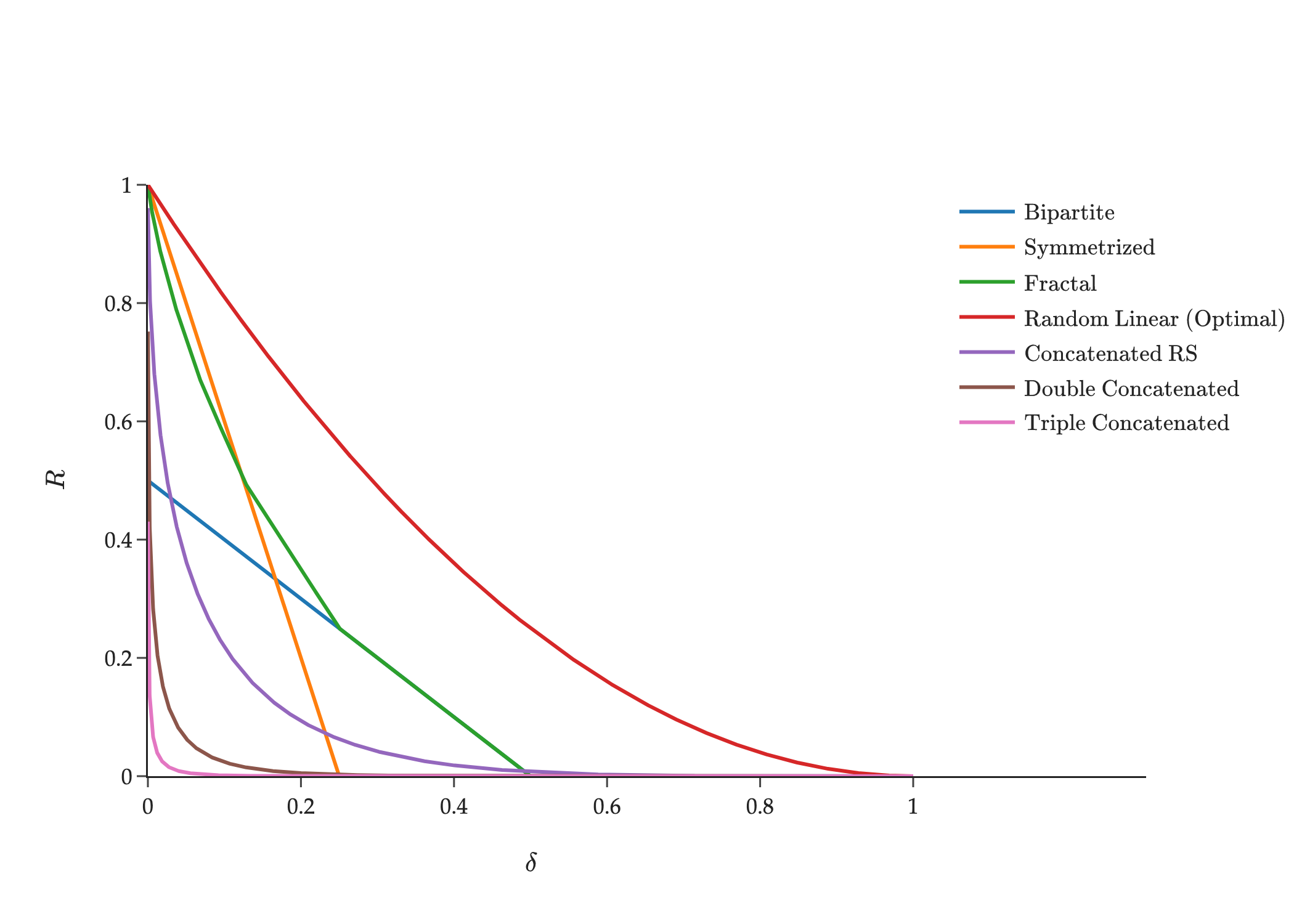
Figure 1: $R$ vs. $\delta$ for graph codes.

1.3 Concluding thoughts and questions

The most interesting question in this context is to get explicit constructions of graph codes with optimal $R$ vs $\delta$ tradeoff. While we have seen a number of constructions achieving nontrivial parameters in various regimes, it would even be interesting to get the right asymptotic behavior for the endpoints with $\delta$ approaching $1$ or with $R$ approaching $1$. The setting of large $\delta$ (including $\delta=1-o(1)$) seems especially challenging, given the connection with the notorious problem of constructing Ramsey graphs.

Another interesting question is to get decoding algorithms for graph codes. For a certain graph code $C$, if we are given a graph that is promised to be close in graph distance to some graph $G$ in $C$. Then, can we efficiently find $G$?

As mentioned earlier, error-correcting graph codes are an instance of the problem of designing error-correcting codes for more general error patterns – where we have $m$ coordinates and various subsets $S_{i}\subseteq[m]$ such that changing all the values in coordinates of a single $S_{i}$ counts as a single corruption. It would be interesting to develop this theory – to both find the limits of what is achievable and to develop techniques for constructing codes against this error model.

Finally, there are many other themes from classical coding theory that could make sense to study in the context of graph codes and graph distance, including in the context of sublinear time algorithms. It would be interesting to explore this.

Organization of this paper:

We set up basic notions in Section 2, and study combinatorial properties of graph codes in Section 3 before turning our attention to explicit constructions. In Section 4, we study some simple explicit constructions of low rate and distance. In Sections 5 and 6, we construct asymptotically good codes with high rate and high distance respectively. Finally, in Section 7, we show explicit constructions of graph codes with very high distance.

2 Graph codes: Basics

All graphs in this section are given by the set of their edges on the vertex set $[n]$. We use $\tau(G)$ is the size of the minimum vertex cover of any graph $G$. For a subset $S\subseteq[n]$, we use $G[S]$ to denote the subgraph of $G$ induced by the vertex set $S$. We define the crucial parameter that defines our graph code.

Definition 2.1 (Graph distance and relative graph distance).

• The graph distance between two graphs $G$ and $H$, denoted by $\operatorname{d_{graph}}(G,H)$, is the smallest $d\in\mathbb{N}$ such that there is a set $S\subseteq[n]$, $|S|=d$, and $G[\overline{S}]=H[\overline{S}]$.

• The relative graph distance, or simply relative distance, between $G$ and $H$ is denoted by $\delta_{\text{graph}}(G,H)$, and is the quantity $\frac{\operatorname{d_{graph}}(G,H)}{n}$.

We remark that in the above definition, we require that the graphs $G[\overline{S}]$ and $H[\overline{S}]$ be identical and not just isomorphic. Lemma 2.3 describes several equivalent characterizations of graph distance.

Definition 2.2 (Graph code).

We say that a set $C\subseteq 2^{\binom{[n]}{2}}$ is a graph code on $[n]$ with distance $d$ if for every pair of graph $G,H\in C$, we have that $\operatorname{d_{graph}}(G,H)\geq d$.

• The rate of $C$, denoted by $R_{C}$, is the quantity $\frac{\log_{2}(|C|)}{\binom{n}{2}}\geq\frac{2\log_{2}(|C|)}{n^{2}}$.

• The distance (resp. relative distance) of $C$, denoted by $d_{C}$ (resp. $\delta_{C}$), is the quantity $\min_{\begin{subarray}{c}G,H\in C\\ G\neq H\end{subarray}}\operatorname{d_{graph}}(G,H)$ (resp. $\min_{\begin{subarray}{c}G,H\in C\\ G\neq H\end{subarray}}\delta_{\text{graph}}(G,H)$).

We may associate, with each graph $G$, its adjacency matrix $A_{G}$. Moreover, we may consider $A_{G}$ as an element of the vector space $\mathbb{F}_{2}^{\binom{n}{2}}$. For two graphs $G$ and $H$, we observe that $A_{G\Delta H}=A_{G}-A_{H}$. We say that a graph code $C$ is linear if there is a subspace $V\leq\mathbb{F}_{2}^{\binom{n}{2}}$ such that $C=\{G~{}|~{}A_{G}\in V\}$. When there is no confusion, we will abuse notation and use $C$ to refer to the code, as well as the subspace. So for a linear graph code $C$, we have $R_{C}=\frac{\dim(C)}{\binom{n}{2}}$. If $A$ is a $n\times n$ matrix and $S,T\subseteq[n]$, let $A_{S,T}$ be the sub-matrix indexed by $S$ on the rows and $T$ on the columns.

Lemma 2.3 (Alternate characterizations of $\operatorname{d_{graph}}$).

Suppose $G$ and $H$ are graphs on the same vertex set. Then

1. $\operatorname{d_{graph}}(G,H)$ is the minimum vertex cover size of $G\Delta H$.

2. $\operatorname{d_{graph}}(G,H)$ is the minimum number of vertices whose neighborhoods you need to edit to transform $G$ into $H$

3. $\operatorname{d_{graph}}(G,H)$ is the minimum number of vertices whose neighborhoods you need to edit to transform $G\Delta H$ into the empty graph.

4. $\operatorname{d_{graph}}(G,H)$ is the minimum $d$ such that there exists a set $S\subseteq[n]$ of size $d$ such that $(A_{G}-A_{H})_{\overline{S},\overline{S}}=\mathbf{0}$. That is, removing the rows and columns in $S$ from $A_{G}-A_{H}$ yields the all-zeros matrix.

3 Combinatorics of $R$ vs. $\delta$

As with other objects in the theory of error-correcting codes, the first question we seek to answer relates to the optimal rate-distance tradeoff. For $x\in[0,1]$, we use $h_{2}(x)=-x\log_{2}x-(1-x)\log_{2}(1-x)$ to denote the binary entropy function.

Lower bound on rate: Random construction.

Proposition 3.1.

There is a linear graph code with dimension at least

$$\max\left\{\binom{n(1-\delta)}{2}-h_{2}(\delta)n-2,0\right\}$$

and relative distance at least $\delta$.

Proof.

We only consider the case when $\binom{n(1-\delta)}{2}-H(\delta)n-2>0$, and prove this by a probabilistic construction. Consider the $\mathbb{F}_{2}$-linear space $C=\langle A_{G_{1}},\ldots,A_{G_{d}}\rangle$, where each $G_{i}$ is chosen independently chosen from the distribution of the Erdös-Rényi random graph $\mathbf{G}_{n,1/2}$, and $d=\binom{n(1-\delta)}{2}-h_{2}(\delta)n-2$. We have

$$\Pr\left(|C|=2^{d}\right) =\prod_{i=2}^{d}\Pr\left(A_{G_{i}}\not\in\langle A_{G_{1}},\ldots,A_{G_{i-1}}\rangle\right)$$

$$=\prod_{i=2}^{d}\left(1-2^{i-\binom{n}{2}}\right)$$

$$\geq 1-\sum_{i=2}^{d}2^{i-\binom{n}{2}}$$

$$\geq 1-2^{d-\binom{n}{2}+1}$$

$$\geq\frac{1}{2}.$$

For any $\overline{\alpha}=(\alpha_{1},\ldots,\alpha_{d})\in\mathbb{F}_{2}^{d}\setminus\{\mathbf{0}\}$, the graph $H_{\overline{\alpha}}$ represented by the adjacency matrix $\sum_{i=1}^{d}\alpha_{i}G_{i}$ has the same law as $\mathbf{G}_{n,\frac{1}{2}}$. So, for any $\overline{\alpha}\neq\mathbf{0}$, we have

$$\Pr(\tau(H_{\overline{\alpha}})\leq\delta n)\leq\binom{n}{\delta n}\cdot 2^{-\binom{n(1-\delta)}{2}}\leq 2^{-\binom{n(1-\delta)}{2}+h_{2}(\delta)n}.$$

Since $C$ is a linear space, we have for $H_{i},H_{j}\in C$, that $H_{i}\Delta H_{j}\in C$. So by the Union bound, and using the fact that $|C|\leq 2^{d}$, we have

$$\Pr\left(\exists\overline{\alpha},\overline{\beta}\in\mathbb{F}_{2}^{d}~{}|~{}\tau(H_{\overline{\alpha}}\Delta H_{\overline{\beta}})\leq\delta n\right) =\Pr\left(\exists\overline{\alpha}\in\mathbb{F}_{2}^{d}\setminus\{\mathbf{0}\}~{}|~{}\tau(H_{\overline{\alpha}})<\delta n\right)$$

$$\leq|C|\cdot 2^{-\binom{n(1-\delta)}{2}+h_{2}(\delta)n}$$

$$\leq\frac{1}{4}.$$

So, by the Union bound, we have that with probability at least $1/4$, $C$ has dimension $\binom{n(1-\delta)}{2}-h_{2}(\delta)n-2$, and relative graph distance $\delta$. ∎

Upper bound on rate: Singleton Bound.

Proposition 3.2.

Any graph code with relative distance $\delta$ has size at most $\binom{n(1-\delta)+1}{2}$.

Proof.

Consider any graph code $C$ of relative distance $\delta$. Let $A\subseteq[n]$ be any subset of at most $\delta n-1$ vertices. For any two distinct $G_{1},G_{2}\in C$, we have that the graphs induced on the vertices outside $A$, $G_{1}[[n]\setminus A]$ and $G_{2}[[n]\setminus A]$, are different. Indeed, since otherwise, $A$ is a vertex cover of $G_{1}\Delta G_{2}$, contradicting the relative distance assumption. So, we have that

$$|C|\leq 2^{\binom{n(1-\delta)+1}{2}}.$$

∎

Let us note a couple of interesting corollaries of Propositions 3.1 and 3.2.

Corollary 3.3.

Let $r_{\delta}$ be the largest rate for a graph code on $[n]$ of relative distance $\delta\in(0,1)$. Then

$$r_{\delta}=(1-\delta)^{2}+O(1/n).$$

Corollary 3.4.

Let $\delta=1-c\cdot\frac{\log n}{n}$ where $c>2$. Then, there is a linear graph code of dimension at least $\Omega(\log^{2}n)$ with relative distance at least $\delta$.

4 Explicit graph codes from rank metric codes

In this section, we will construct explicit and asymptotically good graph codes (codes with constant rate and distance) from rank metric codes.

Definition 4.1 (Rank Metric codes).

A collection of matrices $C\subseteq\mathbb{F}_{q}^{m\times n}$ is called a rank metric code with rank $r$ if every pair $M,N\in C$ satisfy $\operatorname{rank}(M-N)\geq r$.

Code 4.2 (Gabidulin Rank Metric Code $\text{Gab}(n,\delta)$  [Gab85]).

The Gabidulin Code with parameters $n$ and $\delta$, $\text{Gab}(n,\delta)\subseteq\mathbb{F}_{2}^{n\times n}$ is a strongly explicit linear rank metric code of dimension $n^{2}(1-\delta)$ with rank $\delta n$.

Note that more general Gabidulin codes exist (ones over non-square matrices and fields other than $\mathbb{F}_{2}$), but we will only need square matrices over $\mathbb{F}_{2}$ for the applications here. One significant advantage of using Gabidulin codes is that their construction can be made to be strongly explicit, i.e., each adjacency of a graph from the code may be outputted in $\text{polylog}(n)$ time.

Lemma 4.3.

Let $G$, $H$ be graphs on the same vertex set. Then

$$\operatorname{d_{graph}}(G,H)\geq\operatorname{rank}(A_{G}-A_{H})/2.$$

Proof.

Let $A=A_{G}-A_{H}$. Suppose $\operatorname{d_{graph}}(G,H)=d$. Then there exists $S\subseteq[n]$ of size $d$ such that removing the rows in $S$ and columns in $S$ from $A$ yields the 0 matrix. Since removing a single row or column decreases the rank by at most 1, and we remove $d$ rows and $d$ columns, $\operatorname{rank}(A)=\operatorname{rank}(A_{G}-A_{H})=\operatorname{d_{rank}}(A_{G},A_{H})\leq 2d$ ∎

Lemma 4.4.

Let $G,H$ be bipartite graphs on the same vertex set and the same bipartition with bi-adjacency matrices $B_{G}$, and $B_{H}$, respectively. Then

$$\operatorname{d_{graph}}(G,H)\geq\operatorname{rank}(B_{G}-B_{H}).$$

Proof.

Let $B=B_{G}-B_{H}$ be the bi-adjacency matrix of $G-H$. Suppose $\operatorname{d_{graph}}(G,H)=d$. Then, we can clear the neighborhoods of $d$ vertices to get to the empty graph. Clearing the neighborhood of a single vertex in $G-H$ corresponds to removing a single row or column of $B$. Then, again, since removing a single row or column decreases the rank by at most 1, $\operatorname{rank}(B)=\operatorname{rank}(B_{G}-B_{H})\leq d$ ∎

4.1 Gabidulin Codes as graph codes

The first attempt for a strongly explicit graph is to use all elements of a Gabidulin code as bi-adjacency matrices of bipartite graphs.

Code 4.5 (Bipartite Gabidulin Graph Code $C_{\mathrm{Bipartite}}(n,\delta)$).

Let $n$ be a positive integer and $\delta<1/2$. Define

$$C_{\mathrm{Bipartite}}(n,\delta)=\left\{\begin{bmatrix}0&B\\ B^{T}&0\end{bmatrix}:B\in\text{Gab}(n/2,2\delta)\right\}.$$

Theorem 4.6.

Let $\delta\in(0,1/2)$, and $n$ be a positive integer. Then, the graph code $C_{\mathrm{Bipartite}}(n,\delta)$ is a strongly explicit linear graph code with rate $1/2-\delta+o(1)$ and relative distance at least $\delta$.

Proof.

The claim about distance follows from Lemma 4.4. The rate of $C_{\mathrm{Bipartite}}(n,\delta)$ is $\frac{(1-2\delta)(n/2)^{2}}{\binom{n}{2}}=1/2-\delta+o(1)$ ∎

Thus, these codes are already asymptotically good graph codes. However, they only provide graph codes with distance and rate at most $1/2$. In order to overcome this, our next attempt is to choose only matrices from a Gabidulin code that correspond to adjacency matrices of (not necessarily bipartite) graphs.

4.2 An explicit construction for high rate: Symmetric rank metric codes

Our first construction for achieving high rate is based on taking matrices in the Gabidulin code that correspond to adjacency matrices (i.e., they are symmetric and have zeroes on the diagonal).

Code 4.7 (Symmetric Gabidulin Code $C_{\mathrm{Symmetrized}}(n,\delta)$).

For $\delta<1/4$, let us define the family of codes

$$C_{\mathrm{Symmetrized}}(n,\delta)=\left\{A:A\in\text{Gab}(n,2\delta)\text{ and }A\text{ is symmetric and has zeros on the diagonal}\right\},$$

Theorem 4.8.

The graph code $C_{\mathrm{Symmetrized}}(n,\delta)$ is an explicit linear graph code with rate at least $1-4\delta-o(1)$ and relative distance at least $\delta$.

Proof.

The claim about distance follows from Lemma 4.3 by observing that $C_{\mathrm{Symmetrized}}(n,\delta)\subseteq\text{Gab}(n,2\delta)$.

Note that $\text{Gab}(n,2\delta)$ is a linear code with dimension $k=(1-2\delta)n^{2}$. Let $B_{1},...,B_{k}$ be a basis for $G_{n,2\delta}$. Then, restricting $A=\sum_{i=1}^{k}\lambda_{i}B_{i}$ to be symmetric and zero diagonal imposes $\binom{n+1}{2}$ many $\mathbb{F}_{2}$-linear constraints on the space of possible $\vec{\lambda}=(\lambda_{1},\ldots,\lambda_{k})\in\mathbb{F}_{2}^{k}$. Thus, the space of $\vec{\lambda}$ such that $\sum_{i=1}^{k}\lambda_{i}B_{i}$ is symmetric and has zeros on the diagonal has dimension $k-\binom{n+1}{2}$. So the rate is at least

$$\frac{n^{2}(1-2\delta)-\binom{n+1}{2}}{\binom{n}{2}}=1-4\delta-o(1).$$

∎

This solves one of the problems pointed out previously by giving an explicit family of asymptotically good graph codes for any rate. However, the problem now becomes that this construction only guarantees a family of codes for $\delta<\frac{1}{4}$. Furthermore, it is unclear how to make this construction strongly explicit. To address the former issue, we have to develop a new approach, which we do in a later section. We address the latter issue now, at the cost of a slightly worse rate-distance tradeoff.

5 Explicit graph codes for high rate: Fractal Rank Metric Codes

Code 5.1 (Fractal Rank Metric Code $C_{\mathrm{Fractal}}(n,h,\delta)$).

For an integer $h$, $\delta<\frac{1}{2^{h}}$, let us define the following family of codes.

Let $G_{1},...,G_{h}$ be a sequence of Gabidulin codes, where for each $i\in[h]$, $G_{i}=\text{Gab}(n_{i},\delta_{i})$, where $n_{i}=n/2^{i}$, and $\delta_{i}=\delta 2^{i}$.

We define a sequence of codes $\{C_{i}\}_{i\in[h]}$ as follows.

$$C_{k}=\begin{cases}\left\{\begin{bmatrix}0&A\\ A^{T}&0\\ \end{bmatrix}:A\in G_{h-k+1}\right\}&k=1\\ \\ \left\{\begin{bmatrix}B&A\\ A^{T}&C\\ \end{bmatrix}:A\in G_{h-k+1},B,C\in C_{k-1}\right\}&k>1\end{cases}$$

Let $C_{\mathrm{Fractal}}(n,h,\delta)=C_{h}$.

For example, one element of $C_{\mathrm{Fractal}}$ with $h=3$ is illustrated in Figure 2.

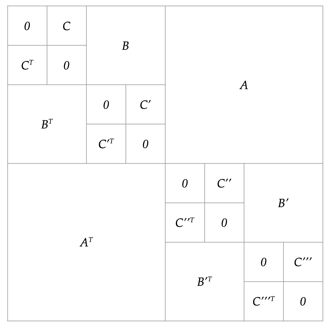
Figure 2: An element of $C_{\mathrm{Fractal}}$ for $h=3$. Note that $A\in G_{1},B,B^{\prime}\in G_{2},C,C^{\prime},C^{\prime\prime},C^{\prime\prime\prime}\in G_{3}$

Theorem 5.2.

Let $n\in\mathbb{N},h\in\mathbb{Z}^{+}$, and $\delta$ be such that $0<\delta<\frac{1}{2^{h}}$, then $C_{\mathrm{Fractal}}(n,h,\delta)$ is a strongly explicit code linear code with distance $\delta$, and rate $1-2^{-h}-h\delta$.

Proof.

Let $C=C_{\mathrm{Fractal}}$. First, note that $C$ is strongly explicit since each of the component Gabidulin codes are strongly explicit.

Distance.

Let $A$ be any non-zero codeword. Then $A$ has some non-zero vertex-induced bipartite subgraph with bi-adjacency matrix coming from one of the Gabidulin codes $G_{1},...,G_{h}$. Since we defined $\delta_{i}=\delta 2^{i}$, each of the $G_{i}$ is a rank metric code with absolute distance at least $\delta n$. Thus, by Lemma 4.4, $\operatorname{d_{graph}}(A,\mathbf{0})\geq\delta$.

Rate.

Any codeword in $C$ is made from exactly $2^{i-1}$ codewords from $G_{i}$, and $|G_{i}|=2^{\left(n/2^{i}\right)^{2}(1-\delta_{i})}$. Thus the total number of codewords in $C$ is

$$\prod_{i\in[h]}\left(2^{\left(n/2^{i}\right)^{2}(1-\delta_{i})}\right)^{2^{i-1}}=2^{n^{2}\sum_{i\in[h]}2^{-i-1}(1-\delta_{i})}.$$

The rate (as a graph code) is then at least

$$\sum_{i\in[h]}2^{-i}(1-\delta_{i}) =\sum_{i\in[h]}2^{-i}(1-\delta 2^{i})$$

$$=\sum_{i\in[h]}\left(2^{-i}-\delta\right)$$

$$=1-2^{-h}-h\delta.$$

∎

Taking $h=O(\log(1/\delta))$, $C_{\mathrm{Fractal}}(n,h,\delta)$ has a rate distance tradeoff of $R=1-O(\delta\log(1/\delta))$.

This code is strongly explicit and can get rate very close to $1$ by picking large $h$ and small $\delta$. On the other hand, this code can only be constructed for $\delta<1/2$. Next, we will see constructions for $\delta=1-o(1)$, and asymptotically good codes for constant $\delta$ close to $1$.

6 Explicit graph codes for high distance: Concatenated Codes

We now turn to constructing asymptotically good graph codes with relative distance $\delta>1/2$.

Instead of getting graph distance via the rank metric, in this section, we show that it is also possible to get graph distance from Hamming distance. To do this, we will use the Tensor Product Code introduced by [Wol65], where elements of the code are matrices where all rows and columns are codewords over some base code. Since, eventually, we need to obtain matrices that are adjacency matrices for undirected graphs, we will also need the matrices to be symmetric and zero-diagonal.

Definition 6.1.

[Symmetric Tensor Code with Zeros on the Diagonal] Let $C$ be a code over $\mathbb{F}_{q}$. The symmetric tensor code with zeros on the diagonal built on $C$ denoted $\mathrm{STCZD}(C)$ is the set of matrices $A$ over $\mathbb{F}_{q}^{n\times n}$ such that (1) $A$ is symmetric, (2) the rows and columns of $A$ are codewords of $C$, and (3) the entries on the diagonal are all 0.

Properties of elements of Tensor Product Codes that are symmetric and zero-diagonal were also previously studied, in the context of constructing a gap-preserving reduction from SAT to the Minimum Distance of a Code problem, by Austrin and Khot [AK14].

We will also define another notion of distance that will be useful later on.

Definition 6.2 (Directed graph distance).

Let $A$, and $B$ be $n\times n$ matrices over some field. Define the directed graph distance denoted $\operatorname{d_{directed}}(G,H)$ to be the minimum $d$ such that there exists sets $S,T\subseteq[n]$ of size $d$ where $(A-B)_{\overline{S},\overline{T}}=\mathbf{0}$.

For weighted, directed graphs, $G$, and $H$, abbreviate $\operatorname{d_{directed}}(A_{G},A_{H})=\operatorname{d_{directed}}(G,H)$. To better distinguish between $\operatorname{d_{directed}}$ and $\operatorname{d_{graph}}$, we sometimes refer to $\operatorname{d_{graph}}$ as the undirected graph distance.

When $G$ and $H$ are weighted directed graphs, $\operatorname{d_{directed}}(A_{G},A_{H})$ can be viewed as the minimum $d$ such that you can go from $G$ to $H$ by editing the incoming edges of $d$ vertices and the outgoing edges of $d$ vertices.

The main difference between directed and undirected graph distance is that directed graph distance allows the subset of rows and the subset of columns to be edited to be different. Insisting that $S=T$ in the definition for directed graph distance, recovers the undirected graph distance. From this, it easily follows that if $G$ and $H$ are undirected graphs, then $\operatorname{d_{directed}}(G,H)\leq\operatorname{d_{graph}}(G,H)$. Thus, to find codes with high graph distance, it suffices to find codes with large directed graph distance, where all the elements are adjacency matrices of undirected, unweighted graphs (i.e., 0/1 matrices that are symmetric and zero diagonal). Note that when discussing rate directed graph codes $C$, we are referring to the quantity $\log_{q}(|C|)/n^{2}$ instead of $\log_{q}(|C|)/\binom{n}{2}$.

In the next lemma, we show several properties of $\mathrm{STCZD}(C)$. Most importantly, the Hamming distance of $C$ translates to the directed graph distance of $\mathrm{STCZD}(C)$.

Lemma 6.3.

Let $C$ be a linear $[n,k,d]_{q}$-code, then $\mathrm{STCZD}(C)\subseteq\mathbb{F}_{q}^{n\times n}$ is linear, has dimension at least $\binom{k+1}{2}-n$, and has directed graph distance $d$.

Proof.

Let $C$ be a linear $[n,k,d]_{q}$-code, and let $C^{\prime}=\mathrm{STCZD}(C)$. $C^{\prime}$ is linear because $C$ is linear, and the sum of symmetric matrices is symmetric.

WLOG, we assume that $C$ is systematic, i.e., it has $k\times n$ generator matrix $G=[I|A]$, where $I$ is the $k\times k$ identity and $A$ is a $k\times(n-k)$ matrix. Then, for every $X\in\mathbb{F}_{q}^{k\times k}$, the following has rows and columns belonging to $C$

$$G^{T}XG=\begin{bmatrix}X&XA\\ A^{T}X&A^{T}XA\\ \end{bmatrix}.$$

Furthermore, $G^{T}XG$ is symmetric and has zeros on the diagonal iff $X$ is symmetric, $X$ has zeros on the diagonal, and $A^{T}XA$ has zeros on the diagonal. This imposes $\binom{k+1}{2}+(n-k)$ linear constraints on the entries of $X$. Thus, the subspace of $X$ for which $G^{T}XG\in C^{\prime}$ has dimension at least $k^{2}-\binom{k+1}{2}-(n-k)=\binom{k+1}{2}-n$.

Since $C^{\prime}$ is linear, to show the distance property, it suffices to show that $\operatorname{d_{directed}}(A,\mathbf{0})\geq d$ for every non-zero $A\in C^{\prime}$. Let $A\in C^{\prime}$ be a non-zero element of $C^{\prime}$, we’ll show that for any $S,T\subseteq[n]$, with $|S|<d$, and $|T|<d$, $A_{\overline{S},\overline{T}}\neq\mathbf{0}$.

Since $A$ is non-zero, there is some non-zero entry $A_{ij}$. Since the rows are elements of a linear code of distance $d$, the Hamming weight of the $i$th row is at least $d$. Since $|T|<d$, there is some $j^{\prime}\notin T$ such that $A_{ij^{\prime}}$ is non-zero. Then, the $j^{\prime}$th column is also a non-zero codeword of $C$, so it also has Hamming weight at least $d$. Since $|S|<d$, there is some $i^{\prime}\notin S$ such that $A_{i^{\prime}j^{\prime}}$ is non-zero. Thus, $A_{\overline{S},\overline{T}}\neq\mathbf{0}$. ∎

Remark 1.

A simple calculation shows that if $C$ has constant rate , $R$, then $\mathrm{STCZD}(C)$ has rate $R^{2}/2-o(1)$ as a directed graph code.

Given this lemma (and using the fact that $\operatorname{d_{graph}}\geq\operatorname{d_{directed}}$), for any binary code $C\subseteq\mathbb{F}_{2}^{n}$ with rate $R$ and relative distance $\delta$, $\mathrm{STCZD}(C)$ is a (undirected) graph code with rate $R^{2}-o(1)$, and relative distance $\delta$. Thus, if $C$ has rate distance trade off $R=f(\delta)$, then $\mathrm{STCZD}(C)$ has rate distance trade off $R=f(\delta)^{2}-o(1)$. Immediately, we get that taking the $\mathrm{STCZD}$ of any asymptotically good binary code, yields an asymptotically good graph code.

There are two problems with this construction. Firstly, these codes may not be strongly explicit, and secondly, the Plotkin bound [Plo60] implies that any binary code with distance $>1/2$ has vanishing rate. So this falls short of our goal of obtaining strongly explicit, asymptotically good codes with $\delta>1/2$.

We will address the the first problem by showing that if the base code is a Reed Solomon code [RS60], then there is a large subcode that is strongly explicit.

Code 6.4 (Reed Solomon Code $\mathrm{RS}(n,R,q)$ [RS60]).

The Reed Solomon Code with parameters $n$, $R$, and $q$, where $q\geq n$, is a code over $\mathbb{F}_{q}^{n}$ with rate $R$ and distance $1-R$.

Lemma 6.5.

Let $C\in\mathrm{RS}(n,R,q)$ where $Rn=k-1$. Then, there exists a strongly explicit subcode $S\subseteq\mathrm{STCZD}(C)$ such that the dimension of $S$ is at least $\binom{k-1}{2}$.

Proof.

Essentially, we will evaluate symmetric polynomials that are a multiple of $(X-Y)^{2}$ on a $n\times n$ grid.

Suppose $h(X,Y)$ is a symmetric polynomial of individual degree at most $k-3$, and let $M$ be the evaluations of $f(X,Y)=(X-Y)^{2}h(X,Y)$ on a $n\times n$ grid. $M$ is symmetric and has zeros on the diagonal. Furthermore, for a fixed value, $y$, $f(X,y)$ is a univariate polynomial in $X$ of degree at most $k-1$, and hence the column indexed by $y$ is an element of a Reed Solomon code of dimension $k$, and block length $n$. Similarly, the rows are also elements of the same code. Thus $M\in\mathrm{STCZD}$.

Let $S$ be the space of bivariate symmetric polynomials of degree at most $k-3$. For $a,b\in\mathbb{N}$, define polynomials $p_{a,b}(X,Y)=X^{a}Y^{b}+X^{b}Y^{a}$. Notice that $p_{a,b}$ is symmetric, and furthermore the set

$$\{p_{a,b}:0\leq a<b\leq k-3\}\cup\{X^{i}Y^{i}:i\in\{0,1,...,k-3\}\},$$

is linearly independent. Thus $\dim(S)=\binom{k-2}{2}+k-2=\binom{k-1}{2}$, as desired.

∎

To extend this construction to the setting of $\delta>1/2$, we use the concatenation paradigm from standard error-correcting code theory, initially introduced by Forney [For65].

We will start with a code over a large alphabet and then concatenate with an inner code, which will be an optimal directed graph code.

Lemma 6.6.

For any $\epsilon>0$, and sufficiently large $n$, for any $k<\epsilon^{2}n^{2}-2n$, there exists a linear directed graph code over $\mathbb{F}_{2}$ of dimension $k$ and distance at least $(1-\epsilon)n$.

The proof is standard and similar to that of Proposition 3.1. So we will omit it.

Code 6.7 (Optimal Directed Graph Code $\mathrm{Opt}(\epsilon,n,k)$).

Require $k<\epsilon^{2}n^{2}-2n$. Refer to a code with the properties in Lemma 6.6 as $\mathrm{Opt}(\epsilon,n,k)$.

6.1 Symmetric concatenation

Since our inner code is not guaranteed to be symmetric, simply replacing each field element in the outer code with its encoding might result in an asymmetric matrix. To remedy this, we transpose the encoding for entries below the diagonal. This is made formal below.

Definition 6.8 (Symmetric Concatenation).

Let $q,Q$ be prime powers, and $n,N$ be positive integers. Let $C_{out}\subseteq\mathbb{F}_{Q}^{N\times N}$ and $C_{in}\subseteq\mathbb{F}_{q}^{n\times n}$ such that $|C_{in}|=Q$. Define $C_{in}\circ C_{out}\subseteq\mathbb{F}_{q}^{nN\times nN}$ to be the code obtained by taking codewords of $C_{out}$ and replacing each symbol of the outer alphabet with by their encodings under $C_{in}$ if they lie above or on the diagonal, and with the transpose of their encodings if they lie below the diagonal.

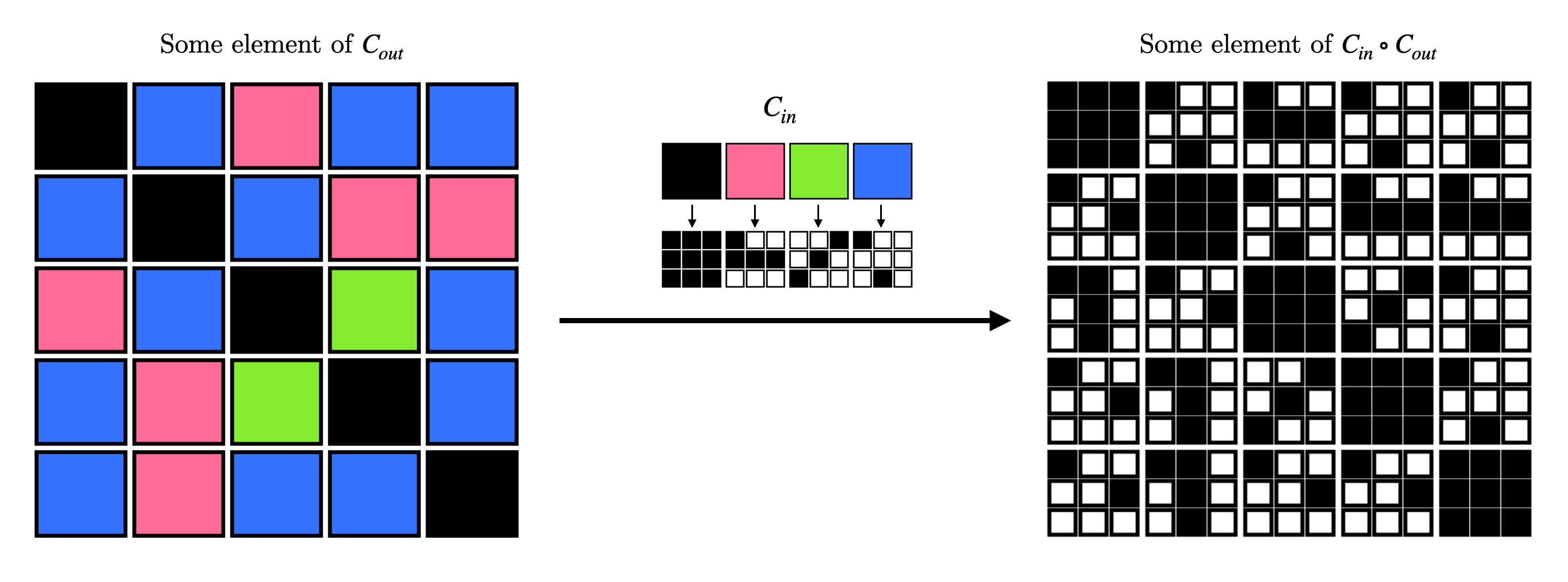
Figure 3: Example of symmetric concatenation. An outer code word is shown on the left, with field elements represented as different colors. The concatenation with the inner code is shown to the right. Black squares represent $0$, and white squares represent $1$s.

Figure 3 visualizes an example of symmetric concatenation. We now show that distance and dimension concatenate exactly like it does for standard error-correcting codes.

Lemma 6.9.

Suppose $C_{in}$ and $C_{out}$ are linear codes as in the previous definition with directed graph distance $d$ and $D$, respectively. Let $k$ be the dimension of $C_{in}$, and $K$ be the dimension of $C_{out}$. Note $|C_{in}|=q^{k}=Q$. Then $C_{in}\circ C_{out}$ is linear and has distance at least $dD$, and dimension $kK$.

Proof.

Let $C=C_{in}\circ C_{out}$. First note that $C_{in}\circ C_{out}$ can be made linear by using a $\mathbb{F}_{q}$-linear map from $\mathbb{F}_{q^{k}}$ to $\mathbb{F}_{q}^{k}$ before encoding with the inner code.

Consider a non-zero outer codeword $O$, and let $A$ be the codeword after concatenation. Let $S,T\subseteq[nN]$ be of size less than $dD$. We’ll show that $A_{\overline{S},\overline{T}}\neq\mathbf{0}$. Partition $A$ into $N\times N$ blocks, where the $(I,J)$’th block for $I,J\in[N]$, is the $n\times n$ matrix encoding the symbol at $O_{IJ}$. Identify the indices $[nN]$ with $[N]\times[n]$ where the tuple $(I,i)$ corresponds to the $i$’th index in the $I$’th block.

For $I\in[N]$, let $S_{I}=\{i\in[n]:(I,i)\in S\}$ be the set rows in $S$ in the $I$’th block. Define $T_{J}$ similarly. Let $S_{\geq}=\left\{I\in[N]:|S_{I}|\geq d\right\}$, be the set of blocks in which there are at least $d$ elements in $S$, and similarly define $T_{\geq}$, $S_{<}$, and $T_{<}$.

Since $\sum_{I\in[N]}|S_{I}|<dD$, $\sum_{J\in[N]}|T_{J}|<dD$, we have $|S_{\geq}|<D$, and $|T_{\geq}|<D$. Since the outer code has directed distance $D$, $O_{S_{<},T_{<}}\neq\mathbf{0}$, so there exists $I\in S_{<}$, and $J\in T_{<}$ such that $O_{I,J}$ is non-zero. So, the $(I,J)$’th block of $A$ is a non-zero codeword or the transpose of a non-zero codeword of $C_{in}$. Let us call it $X$, and suppose that $X\in C_{in}$.

Since $|S_{I}|<d$, and $|T_{J}|<d$, and the inner code has distance at least $d$, we have that $X_{\overline{S_{I}},\overline{T_{J}}}\neq\mathbf{0}$. To finish the proof, note that $\operatorname{d_{directed}}(X,\mathbf{0})=\operatorname{d_{directed}}(X^{T},\mathbf{0})$ by switching the roles of $S$ and $T$ in the definition of directed graph distance.

For the claim about dimension, note that the number of codewords in $C$ is the number of codewords in $C_{out}$, which is $Q^{K}$. The dimension of $C$ is then $K\log_{q}(Q)=Kk$. ∎

Additionally, it is clear from the definition of symmetric concatenation that if $C_{out}$ is symmetric and zero-diagonal, so is $C_{in}\circ C_{out}$.

Remark 2.

Lemma 6.9 also holds for the standard definition of concatenation (without transposing blocks below the diagonal). However, we will not need this fact.

6.2 Concatenated graph codes

We can instantiate the concatenated code using Reed Solomon codes.

Code 6.10 (Concatenated Code $C_{\mathrm{RS}}(\epsilon,n,k,N,\rho)$).

Let $Q=2^{k}$ be the size of the alphabet of the outer code. Let $\epsilon,\rho\in(0,1)$, and $n,k,N$, to be integers satisfying $k<\epsilon^{2}n^{2}-2n$, and $N\leq Q$. Then,

$$C_{\mathrm{RS}}=\mathrm{Opt}(\epsilon,n,k)\circ\mathrm{STCZD}(\mathrm{RS}(N,\rho,Q)).$$

The following theorem follows directly from Lemmas 6.3 and 6.9. As a reminder, here we are considering the rate of the codes as a (undirected) graph code.

Theorem 6.11.

Let $\epsilon,n,k,N,\rho$ be parameters satisfying the requirements listed in 6.10.

Then $C_{\mathrm{RS}}(\epsilon,n,k,N,\rho)$ is a graph code with rate $\epsilon^{2}\rho^{2}-o(1)$, and relative distance $(1-\epsilon)(1-\rho)$.

Note that using this construction, we can get asymptotically good codes for any constant rate and distance - including for distances $>1/2$, which was not obtained in any of the previous constructions. We get $R=(1-\sqrt{\delta})^{4}+o(1)$ by setting $\epsilon=\rho$.

One drawback of this construction is that it is not strongly explicit or even explicit. The outer code can be made strongly explicit using Lemma 6.5, however, the inner code was an optimal code which we obtained by a randomized construction. The complexity of searching for such a code by brute force is too large. In particular, the optimal code has dimension $\epsilon^{2}n^{2}$, and block length $n^{2}$. Since we need the size of the code to be equal to the size of the outer alphabet, we have $N=2^{\epsilon^{2}n^{2}}$, so $n=\sqrt{\log(N)}/\epsilon$. Then, there are at least $2^{\epsilon^{2}n^{4}}=2^{\log(N)^{2}/\epsilon^{2}}$ generator matrices to search over. Thus, we cannot find such a code efficiently.

To address this, we reduce the search space by concatenating multiple times. The resulting code will have a slightly worse distance/rate trade-off but will still be asymptotically good for any constant distance or rate.

We also note that $C_{\mathrm{RS}}$ can also be made strongly explicit using a Justensen-like construction. However, although this code is again asymptotically good, it has distance bounded away from 1. We present this construction in the Appendix.

6.3 Multiple concatenation

While concatenating twice suffices to obtain an explicit code, it is not clear that the obtained code is strongly explicit. This may be addressed by concatenating three times, at the cost of slightly weaker parameters. Here, we will also use the tensor product code as a building block. For any linear code $C\subseteq\mathbb{F}_{q}^{n}$, let $\mathrm{TC}(C)$ be the tensor product code of $C$. As a reminder, $\mathrm{TC}(C)$ is the code consisting of matrices $A\in\mathbb{F}_{q}^{n\times n}$ such that each row and each column of $A$ are elements of $C$.

Remark 3.

Suppose $C$ is a linear code with distance $d$ and rate $R$. Then, it follows from the proof of Lemma 6.3 that $\mathrm{TC}(C)$ has directed graph distance at least $d$. It is also well known that $\mathrm{TC}(C)$ has rate $R^{2}$.

Below we present the analysis for triple concatenation.

Code 6.12 (Triple Concatenation $\mathrm{C_{Trip}}(\rho,N)$).

For $\rho\in(0,1)$ and an integer $N$, let $C$ be the subcode of $\mathrm{STCZD}(\mathrm{RS}(N,\rho,N))$ in Lemma 6.5. Then

$$\mathrm{C_{Trip}}=\mathrm{Opt}(N_{3},\rho)\circ\mathrm{TC}(\mathrm{RS}(N_{2},\rho,N_{2}))\circ\mathrm{TC}(\mathrm{RS}(N_{1},\rho,N_{1}))\circ C,$$

where $N_{1},N_{2}$ and $N_{3}$ are picked to make the concatenation work, i.e., $|\mathrm{Opt}(N_{3},\rho)|\geq N_{2}$, and so on.

Notice that only the outer-most code needs to be symmetric and have zero diagonal since we use the symmetric concatenation operation (entries below the diagonal will be transposed). Thus, using the Tensor Product Code for the two middle codes (instead of STCZD) is sufficient and saves a factor of 2 (each time) on the rate.

Theorem 6.13.

Let $N$ be a positive integer and $\rho\in(0,1)$. Then $\mathrm{C_{Trip}}(\rho,N)$ has distance at least $(1-\rho)^{4}$, and rate $\rho^{8}$. Furthermore, $\mathrm{C_{Trip}}(\rho,N)$ is strongly explicit.

Proof.

The claims about rate and distance follow directly from Lemma 6.9.

We’ll now show that this code is strongly explicit. The outermost code $C$ is strongly explicit, and the two codes in the middle built on Reed Solomon codes are also strongly explicit. The idea is that the concatenation steps middle allow us to shrink the alphabet size from $N$ to (less than) $\log(\log(N))$. Searching for optimal codes of this size can be done easily by brute force.

The dimension of $\mathrm{TC}(\mathrm{RS}(N_{1},\rho,N_{1}))$ is $(\rho N_{1})^{2}$, so the number of codewords is $N_{1}^{(\rho_{1}N_{1})^{2}}$, and for the concatenation to work, we need this to be at least $N$. That is, we need $(\rho_{1}N_{1})^{2}\log(N_{1})\geq\log(N)$, which we can get easily by setting $N_{1}=O(\log(N))$. For the same reason, we can take $N_{2}=O(\log\log(N))$.

This is now small enough to do a brute force search for an optimal code. The inner-most code has dimension $\rho^{2}N_{3}^{2}$, so we need $2^{\rho^{2}N_{3}^{2}}=N_{2}$, or $N_{3}=O(\sqrt{\log(N_{2})})$. There are then $\rho^{2}N_{3}^{4}$ possible generator matrices to search over. So the total number of codes we will need to search over is at most $2^{\rho^{2}n^{4}}=2^{O(\log\log\log(N)^{2})}=2^{o(\log\log(N))}=O(\log(N))$. ∎

The tradeoff for this code is then

$$R=(1-\delta^{1/4})^{8}.$$

Thus, we get strongly explicit asymptotically good codes for any constant distance or rate.

If we just wanted explicit codes (instead of strongly explicit), concatenating twice suffices. In particular, the search space for the inner-most code has size

$$2^{O(\log\log(N)^{2})}=2^{o(\log(N))},$$

which is smaller that any polynomial in $N$, but not polylogarithmic. The corresponding tradeoff for the double concatenated code is $R=(1-\delta^{1/3})^{6}$.

7 Explicit graph codes with very high distance: dual-BCH Codes

In this section, we give explicit constructions of graph codes for the setting of very high distance ($\delta=1-o(1)$). As noted earlier, when the complete graph and the empty graph are part of the code, this is a generalization of the problem of constructing explicit Ramsey graphs (i.e., graphs with no large clique or independent set), which corresponds to graph codes of size at least $3$.

Our main result here is an explicit construction of a graph code with distance $1-\frac{n^{\epsilon}}{n^{1/2}}$ and dimension $\Omega(n^{\epsilon}\log n)$, for all $\epsilon\in[0,1/2)$.

Theorem 7.1.

For all $d$, there is a strongly explicit construction construction of a code with dimension $\Omega(d\log n)$ and distance $n-O(d\sqrt{n})$.

In analogy with the situation for Hamming-distance codes, these are the dual-BCH codes of the graph-distance world.

7.1 Warmup: a graph code with dimension $\Omega(\log n)$

As a warmup, we first construct code with distance $1-\frac{1}{n^{\epsilon}}$ with growing dimension.

Let $n=2^{t}$. Let $\mathsf{Tr}:\mathbb{F}_{2^{t}}\to\mathbb{F}_{2}$ denote the finite field trace map. Concretely, it is given by:

$$\mathsf{Tr}(x)=x+x^{2}+x^{4}+\ldots+x^{2^{i}}+\ldots+x^{2^{t-1}}$$

For each $\alpha\in\mathbb{F}_{2^{t}}$, consider the matrix $M_{\alpha}\in\mathbb{F}_{2}^{n\times n}$, where the rows and columns of $M_{\alpha}$ are indexed by elements of $\mathbb{F}_{2^{t}}$, given by:

$$\left(M_{\alpha}\right)_{x,y}=\mathsf{Tr}(\alpha\cdot(x+y)^{3}).$$

Note that each $M_{\alpha}$ is symmetric. Consider the code

Code 7.2.

For $n$ of the form $2^{t}$, let us define the family of codes

$$C_{\mathrm{Warmup}}=\{M_{\alpha}\mid\alpha\in\mathbb{F}_{2^{t}}\}.$$

We have that $C_{\mathrm{Warmup}}$ is a linear code of dimension $t=\log_{2}n$.

Theorem 7.3.

The distance of $C_{\mathrm{Warmup}}$ is at least $1-O(n^{-1/2})$.

Proof.

Fix any $\alpha\in\mathbb{F}_{2^{t}}$. Let $S\subseteq\mathbb{F}_{2^{t}}$ be an arbitrary subset of vertices. It suffices to show that if $S$ is bigger than $\Omega(n^{1/2})=\Omega(2^{t/2})$, then there exist some $x,y\in S$ such that

$$\mathsf{Tr}(\alpha\cdot(x+y)^{3})=1.$$

Suppose not. Then we have:

$$\sum_{x,y\in S}(-1)^{\mathsf{Tr}(\alpha(x+y)^{3})}=|S|^{2}.$$

By Cauchy-Schwarz, we get:

$$|S|^{4} =\left(\sum_{x\in S}\sum_{y\in S}(-1)^{\mathsf{Tr}(\alpha(x+y)^{3})}\right)^{2}$$

$$\leq\left(\sum_{x\in S}\left(\sum_{y\in S}(-1)^{\mathsf{Tr}(\alpha(x+y)^{3})}\right)^{2}\right)\cdot|S|$$

$$\leq\left(\sum_{x\in\mathbb{F}_{2^{t}}}\left(\sum_{y\in S}(-1)^{\mathsf{Tr}(\alpha(x+y)^{3})}\right)^{2}\right)\cdot|S|$$

$$=\left(\sum_{x\in\mathbb{F}_{2^{t}}}\sum_{y_{1},y_{2}\in S}(-1)^{\mathsf{Tr}(\alpha((x+y_{1})^{3}+(x+y_{2})^{3}))}\right)\cdot|S|$$

$$\leq\left(\sum_{y_{1},y_{2}}\left|\sum_{x\in\mathbb{F}_{2^{t}}}(-1)^{\mathsf{Tr}(\alpha((x+y_{1})^{3}+(x+y_{2})^{3}))}\right|\right)\cdot|S|.$$

For $y_{1},y_{2}\in\mathbb{F}_{2^{t}}$, let $P_{y_{1},y_{2}}(X)$ be the polynomial

$$P_{y_{1},y_{2}}(X) =\alpha\cdot\left((X+y_{1})^{3}+(X+y_{2})^{3}\right)$$

$$=\alpha\cdot\left((y_{1}+y_{2})X^{2}+(y_{1}^{2}+y_{2}^{2})X+(y_{1}^{3}+y_{2}^{3})\right).$$

The key observation is that for most $(y_{1},y_{2})\in S^{2}$, the trace of the polynomial $P_{y_{1},y_{2}}(X)$ is a nonconstant $\mathbb{F}_{2}$-linear function, and thus the inner sum:

$$\sum_{x\in\mathbb{F}_{2^{t}}}(-1)^{\mathsf{Tr}(P_{y_{1},y_{2}}(x))}$$

equals $0$.

Lemma 7.4.

If $P(X)=aX^{2}+bX+c\in\mathbb{F}_{2^{t}}[X]$, then

$$\mathsf{Tr}\circ P:\mathbb{F}_{2^{t}}\to\mathbb{F}_{2}$$

is a nonconstant $\mathbb{F}_{2}$-linear function unless $a=b^{2}$.

The proof is standard, and we omit it.

By the lemma, we get that there are at most $4|S|$ choices of $(y_{1},y_{2})$ such that the inner sum is non-zero (namely those $(y_{1},y_{2})\in S^{2}$ for which $\alpha(y_{1}+y_{2})=\left(\alpha(y_{1}^{2}+y_{2}^{2})\right)^{2}$, which are few in number by the Schwartz-Zippel lemma).

Thus we get:

$$|S|^{4}\leq 4|S|^{2}\cdot 2^{t},$$

from which we get $|S|\leq O(2^{t/2})$, as desired. ∎

7.2 Larger dimension

We now see how to get graph codes of distance $1-\frac{1}{n^{\epsilon}}$ with $\epsilon<\frac{1}{2}$ and larger rate.

For a polynomial $f(X)\in\mathbb{F}_{2^{t}}[X]$, let $M_{f}$ be $n\times n$ matrix with rows and columns indexed by $\mathbb{F}_{2^{t}}$ for which:

$$\left(M_{f}\right)_{x,y}=\mathsf{Tr}(f(x+y)).$$

Let $W_{d}$ be the $\mathbb{F}_{2^{t}}$-linear space of all polynomials $f(X)$ of the form:

$$f(X)=\sum_{3\leq 2i+1\leq d}\alpha_{i}X^{2i+1},$$

where the $\alpha_{i}\in\mathbb{F}_{2^{t}}$.

Then, let us define our construction.

Code 7.5.

For $n$ of the form $2^{t}$ and $d\leq n^{1/2}$, let us define the family of codes

$$C_{\mathrm{DualBCH}}(n,d)=\{M_{f}:f\in W_{d}\}.$$

Theorem 7.6.

We have that $C_{\mathrm{DualBCH}}(n,d)$ is a linear graph code of distance $1-O\left(dn^{-1/2}\right)$ and dimension $\Omega(dt)=\Omega(d\log n)$.

Proof.

The proof is very similar to the proof of Theorem 7.3. Consider any $M_{f}\in C_{\mathrm{DualBCH}}(n,d)$ with $f\neq 0$. It suffices to show that the independence number of $M_{f}$ is $O(dn^{1/2})$.

Assume that $S\subseteq\mathbb{F}_{2^{t}}$ is an independent set in $M_{f}$. Then

$$|S|^{2}=\sum_{x,y\in S}(-1)^{\mathsf{Tr}(f(x+y))}.$$ (1)

As in the proof of Theorem 7.3, by the Cauchy-Schwartz inequality and some simple manipulations, we get:

$$|S|^{4} \leq\left(\sum_{y_{1},y_{2}\in S}\left|\sum_{x\in\mathbb{F}_{2^{t}}}(-1)^{\mathsf{Tr}(P_{y_{1},y_{2}}(x))}\right|\right)\cdot|S|,$$ (2)

where:

$$P_{y_{1},y_{2}}(X)=f(X+y_{1})-f(X+y_{2}).$$

At this point, we need an upper bound in the inner sum:

$$U_{y_{1},y_{2}}=\left|\sum_{x\in\mathbb{F}_{2^{t}}}(-1)^{\mathsf{Tr}(P_{y_{1},y_{2}}(x))}\right|.$$

To get this, we will invoke the deep and powerful Weil bound:

Theorem 7.7 ([Sch76], Chapter II, Theorem 2E).

Suppose $P(X)\in\mathbb{F}_{2^{t}}(X)$ is a nonzero polynomial of odd degree with degree at most $d$. Then:

$$\left|\sum_{x\in\mathbb{F}_{2^{t}}}(-1)^{\mathsf{Tr}(P(x))}\right|\leq O(d2^{t/2}).$$

We will use this to show that all but a few pairs $(y_{1},y_{2})\in S^{2}$, $U_{y_{1},y_{2}}$ is small.

Lemma 7.8.

For all but $d|S|$ pairs $(y_{1},y_{2})\in S^{2}$,

$$U_{y_{1},y_{2}}\leq O(d2^{t/2}).$$

is at most $d|S|$.

Assuming this for the moment, we can proceed with Equation (2):

$$|S|^{4} \leq\left(d|S|\cdot 2^{t}+|S|^{2}\cdot O(d\cdot 2^{t/2})\right)\cdot|S|$$

$$=d|S|^{2}2^{t}+O(d|S|^{3}2^{t/2}).$$

Thus:

$$|S|^{2}\leq d2^{t}+O(d|S|2^{t/2}),$$

which implies that $|S|\leq O\left(d\cdot 2^{t/2}\right)$, as desired.

∎

Proof of Lemma 7.8

Proof.

Theorem 7.7 only applies to polynomials with odd degree. We first recall a standard trick involving the $\mathsf{Tr}$ map to deduce consequences for arbitrary degree polynomials.

Note that $\mathsf{Tr}(a^{2})=\mathsf{Tr}(a)$ for all $a\in\mathbb{F}_{2^{t}}$, and that every element of $\mathbb{F}_{2^{t}}$ has a square root. Thus for any positive degree monomial $M(X)=\alpha X^{i}$, where $i=j\cdot 2^{k}$ with $j$ odd, the equality:

$$\mathsf{Tr}(M(x))=\mathsf{Tr}(\widetilde{M}(x))$$

for each $x\in\mathbb{F}_{2^{t}}$, where $\widetilde{M}(X)$ is the odd degree monomial given by:

$$\widetilde{M}(X)=\alpha^{1/2^{k}}X^{j}.$$

Extending by linearity, this allows us to associate, to every polynomial $P(X)\in\mathbb{F}_{2^{t}}[X]$, a polynomial $\widetilde{P}(X)$ with

$$\mathsf{Tr}(P(x))=\mathsf{Tr}(\widetilde{P}(x))$$

for all $x\in\mathbb{F}_{2^{t}}$, and where every monomial of $\widetilde{P}(X)$ (except possibly the constant term) has odd degree.

The key observation is that whenever $\widetilde{P}_{y_{1},y_{2}}(X)$ is nonconstant, it has odd degree, and so we can apply the Weil bound. In this case, since:

$$\mathsf{Tr}(P_{y_{1},y_{2}}(x))=\mathsf{Tr}(\widetilde{P}_{y_{1},y_{2}}(x))$$

for each $x\in\mathbb{F}_{2^{t}}$, we get:

$$U_{y_{1},y_{2}} =\left|\sum_{x\in\mathbb{F}_{2^{t}}}(-1)^{\mathsf{Tr}(\widetilde{P}_{y_{1},y_{2}}(x))}\right|$$ (3)

$$\leq O(d\cdot 2^{t/2}),$$ (4)

where the last step follows from the Weil bound (Theorem 7.7).

Thus we simply need to show that there are at most $d|S|$ pairs $(y_{1},y_{2})\in S^{2}$ for which $\widetilde{P}_{y_{1},y_{2}}(X)$ is a constant.

Suppose $f(X)$ has degree exactly $2e+1$. Let $\alpha$ be the coefficient of $X^{2e+1}$ in $f(X)$.

Define $\gamma_{i}(Y)\in\mathbb{F}_{q}[Y]$ by:

$$f(X+Y)=\sum_{j=0}^{2e+1}\gamma_{i}(Y)X^{i}.$$

Note that $\deg(\gamma_{i}(Y))\leq 2e+1-i$. It is easy to check that $\gamma_{2e+1}(Y)=\alpha$ and $\gamma_{2d}(Y)=\alpha Y$.

Then we have:

$$P_{y_{1},y_{2}}(X) =f(X+y_{1})-f(X+y_{2})$$

$$=\sum_{i\leq 2e}\left(\gamma_{i}(y_{1})-\gamma_{i}(y_{2})\right)X^{i}.$$

Then by definition,

$$\widetilde{P}_{y_{1},y_{2}}(X)=\sum_{\begin{subarray}{c}j\leq 2e-1\\ j\mbox{ odd }\end{subarray}}\left(\sum_{\begin{subarray}{c}k\geq 0\\ j2^{k}\leq 2e\end{subarray}}\left(\gamma_{j\cdot 2^{k}}(y_{1})-\gamma_{j\cdot 2^{k}}(y_{2})\right)^{\frac{1}{2^{k}}}\right)X^{j}.$$

We are trying to show that for most $y_{1},y_{2}$, this is nonconstant. We will do this by identifying a monomial of positive degree which often has a nonzero coefficient. Let $e=j_{0}\cdot 2^{k_{0}}$ with $j$ odd. We will focus on the coefficient of $X^{k_{0}}$. It equals:

$$\left(\gamma_{2e}(y_{1})-\gamma_{2e}(y_{2})\right)^{1/{2^{k_{0}+1}}}+\left(\sum_{0\leq k\leq k_{0}}\left(\gamma_{j\cdot 2^{k}}(y_{1})-\gamma_{j\cdot 2^{k}}(y_{2})\right)^{\frac{1}{2^{k}}}\right).$$

By linearity of the map $a\mapsto a^{1/2^{k}}$, this can be expressed in the form $Q(y_{1}^{1/2^{k_{0}+1}},y_{2}^{1/2^{k_{0}+1}})$, where $Q(Z_{1},Z_{2})$ is a bivariate polynomial of degree at most $2e$. Furthermore, using the fact that $\gamma_{2e}(Y)=\alpha Y$, the homogeneous part of $Q(Z_{1},Z_{2})$ of degree $1$ exactly equals:

$$\alpha^{1/2^{k_{0}+1}}(Z_{1}-Z_{2}),$$

which is nonzero. Thus $Q(Z_{1},Z_{2})$ is a nonzero polynomial.

Thus by the Schwartz-Zippel lemma, for $T=\{y^{1/2^{k_{0}+1}}\mid y\in S\}$, there are at most $2e|T|\leq d|S|$ values of $(z_{1},z_{2})\in T^{2}$ such that $Q(z_{1},z_{2})=0$. Thus there are at most $d|S|$ values of $(y_{1},y_{2})\in S^{2}$ for which the coefficient of $X^{k_{0}}$ in $\widetilde{P}_{y_{1},y_{2}}(X)$ is $0$. Whenever it is nonzero, Equation (4) bounding $U_{y_{1},y_{2}}$ applies, and we get the desired result.

∎

8 Appendix

8.1 Justensen-like code

The construction in this example is inspired by the Justensen code [Jus72], which uses an ensemble of codes for the inner code instead of a single inner code. Justensen uses an ensemble known as the Wozencraft Ensemble [Mas63] with the following properties.

Theorem 8.1 (Wozencraft Ensemble).

For every large enough $k$, there exists codes $C^{(1)},C^{(2)},...,C^{(2^{k}-1)}$ over $\mathbb{F}_{2}^{2k}$ with rate $1/2$, where $1-\epsilon$ fraction of them have distance at least $H^{-1}_{2}(1/2-\epsilon)$.

Since our goal is graph distance, we use the $\mathrm{STCZD}$ operation to covert the Wozencraft Ensemble from codes over strings with good Hamming distance to codes of matrices with good graph distance.

Lemma 8.2 (Wozencraft Ensemble Modification).

For any $\epsilon>0$, and large enough $k$, there exists codes $D^{(1)},D^{(2)},...,D^{(2^{k}-1)}$ over $\mathbb{F}_{2}^{2k\times 2k}$. View these as directed graph codes. Then these codes have rate $1/8$, and at least a $1-\epsilon$ fraction of them have distance at least $H^{-1}_{2}(1/2-\epsilon)$.

Proof.

Let $C^{(1)},C^{(2)},...,C^{(N)}$ be the Wozencraft Ensemble. For each $I\in[N]$, define $D^{(I)}=\mathrm{STCZD}(C^{(I)})$. Note that each $D^{(I)}$ is a code over $\mathbb{F}_{2}^{2k\times 2k}$. Note that by lemma Lemma 6.3, each of the codes has rate $1/8$. Since the $\mathrm{STCZD}$ operation translates Hamming distance to directed graph distance, we also have the same guarantee as the original Wozencraft Ensemble - at least $(1-\epsilon)$ fraction of the codes have distance at least $H^{-1}_{2}(1/2-\epsilon)$. ∎

Concatenating $\mathrm{STCZD}(RS)$ with the modified Wozencraft Ensemble in a particular arrangement yields our next construction.

Code 8.3 (Justensen-like $C_{\mathrm{Justensen}}(\epsilon,k,\rho)$).

Require $\epsilon,\rho\in(0,1)$. Let $Q=2^{k}$, and $N=2^{k}-1$.

Let $D^{(1)},D^{(2)},...,D^{2^{k}-1}$ be the modified Wozencraft Ensemble Lemma 8.2.

Then $C_{\mathrm{Justensen}}$ is the code where for each element of $A\in\mathrm{STCZD}(\mathrm{RS}(N,\rho,Q))$, for each $I,J\in[N]$, we replace the symbol at $A_{IJ}$ with its encoding under $D^{(\min(I,J))}$. If $J<I$, we transpose the encoding (to keep the matrix symmetric).

Figure 4 shows where each inner code is applied.

$$\begin{bmatrix}-&D^{(1)}&D^{(1)}&D^{(1)}&D^{(1)}&D^{(1)}\\ D^{(1)T}&-&D^{(2)}&D^{(2)}&D^{(2)}&D^{(2)}\\ D^{(1)T}&D^{(2)T}&-&D^{(3)}&D^{(3)}&D^{(3)}\\ D^{(1)T}&D^{(2)T}&D^{(3)T}&-&D^{(4)}&D^{(4)}\\ D^{(1)T}&D^{(2)T}&D^{(3)T}&D^{(4)T}&-&D^{(5)}\\ D^{(1)T}&D^{(2)T}&D^{(3)T}&D^{(4)T}&D^{(5)T}&-\end{bmatrix}$$

Figure 4: Inner code arrangement for $C_{\mathrm{Justensen}}$

Theorem 8.4.

For any $\epsilon,\rho\in(0,1)$, and $k$, a sufficiently large integer, $C_{\mathrm{Justensen}}(\epsilon,\rho,k)$ is a strongly explicit linear graph code with rate $\rho^{2}/8-o(1)$, and distance at least $(1-\rho-\epsilon)H^{-1}(1/2-\epsilon)$.

Proof.

Let $N=2^{k}-1$, and $n=2k$ be the side lengths of the inner and outer codes, respectively. First note that $C_{\mathrm{Justensen}}$ is a linear graph code over $\mathbb{F}_{2}^{nN\times nN}$, since both the inner and outer codes are linear, and we can apply a $\mathbb{F}_{2}$ linear map from $\mathbb{F}_{2^{k}}\to\mathbb{F}_{2}^{k}$ before encoding with the inner code.

Rate. By Lemma 6.3, the outer code, $\mathrm{STCZD}(\mathrm{RS}(N,\rho,Q))$, has rate $\rho^{2}/2-o(1)$, and by Lemma 8.2, the inner codes have rate $1/8-o(1)$. Thus, the rate is $\rho^{2}/8-o(1)$ as an undirected graph code.

Distance. Let $O$ be a non-zero outer codeword. For convenience, let $d=H^{-1}(1/2-\epsilon)$, and $n=2k$ be the side length of the inner code. We claim the distance is at least $(1-\rho-\epsilon)d$.

Call $I\in[N]$, bad if the distance of $D^{(I)}<d$, and good otherwise. Let $B\subseteq[N]$ be the subset of bad indices. By the guarantee of the Wozencraft ensemble, we know that $|B|<\epsilon N$. Since $O_{IJ}$ gets encoded with $\min(I,J)$, if $I,J\notin B$, then $O_{IJ}$ is encoded with an inner code of distance at least $d$.

Define $S_{I},T_{J}$ as in the proof of Lemma 6.9. Let $S_{\geq}=\{I:|S_{I}|\geq d_{in}\text{ and }I\notin B\}$. Similarly, define $T_{\geq}$. Then $|S_{\geq}|,|T_{\geq}|<(1-\rho-\epsilon)N$. Then $|S_{\geq}\cup B|,|T_{\geq}\cup B<(1-\rho)N$. Since this is less than the outer distance of the code, we have that $O_{IJ}\neq 0$ for some $I\notin S_{\geq}\cup B$, and $J\notin T_{\geq}\cup B$. In other words, $|S_{I}|<d$, $|T_{J}|<d_{in}$, and $O_{IJ}$ is encoded with a code of directed graph distance at least $d$. Thus, by the inner distance, there remains a non-zero element in the $(I,J)$th block outside of $S_{I}$, and $T_{J}$. ∎

References

- [Plo60] M. Plotkin “Binary Codes with Specified Minimum Distance” In IRE Transactions on Information Theory 6.4, 1960, pp. 445–450 DOI: 10.1109/TIT.1960.1057584
- [RS60] I.. Reed and G. Solomon “Polynomial Codes Over Certain Finite Fields” In Journal of the Society for Industrial and Applied Mathematics 8.2, 1960, pp. 300–304 DOI: 10.1137/0108018
- [Mas63] James L Massey “Threshold Decoding”, 1963
- [For65] G David Forney “Concatenated Codes.”, 1965
- [Wol65] J. Wolf “On Codes Derivable from the Tensor Product of Check Matrices” In IEEE Transactions on Information Theory 11.2, 1965, pp. 281–284 DOI: 10.1109/TIT.1965.1053771
- [Jus72] J. Justesen “Class of Constructive Asymptotically Good Algebraic Codes” In IEEE Transactions on Information Theory 18.5, 1972, pp. 652–656 DOI: 10.1109/TIT.1972.1054893
- [Sch76] Wolfgang M. Schmidt “Equations over Finite Fields: An Elementary Approach”, 1976 URL: https://api.semanticscholar.org/CorpusID:119017517
- [Gab85] Ernst Gabidulin “Theory of Codes with Maximum Rank Distance (Translation)” In Problems of Information Transmission 21, 1985, pp. 1–12
- [AK14] Per Austrin and Subhash Khot “A Simple Deterministic Reduction for the Gap Minimum Distance of Code Problem” In IEEE Transactions on Information Theory 60.10, 2014, pp. 6636–6645 DOI: 10.1109/TIT.2014.2340869
- [Alo23] Noga Alon “Connectivity Graph-Codes” In arXiv preprint arXiv:2308.07653, 2023
- [Alo23a] Noga Alon “Graph-codes” In arXiv preprint arXiv:2301.13305, 2023
- [Alo+23] Noga Alon et al. “Structured codes of graphs” In SIAM Journal on Discrete Mathematics 37.1 SIAM, 2023, pp. 379–403
- [Dev] Pat Devlin, Personal Communication