AI-Assisted Dynamic Port and Waveform Switching for Enhancing UL Coverage in 5G NR

Abstract

The uplink of 5G networks allows selecting the transmit waveform between cyclic prefix orthogonal frequency division multiplexing (CP-OFDM) and discrete Fourier transform spread OFDM (DFT-S-OFDM), which is appealing for cell-edge users using high-frequency bands, since it shows a smaller peak-to-average power ratio, and allows a higher transmit power. Nevertheless, DFT-S-OFDM exhibits a higher block error rate (BLER) which complicates an optimal waveform selection. In this paper, we propose an intelligent waveform-switching mechanism based on deep reinforcement learning (DRL). In this proposal, a learning agent aims at maximizing a function built using available throughput percentiles in real networks. Said percentiles are weighted so as to improve the cell-edge users’ service without dramatically reducing the cell average. Aggregated measurements of signal-to-noise ratio (SNR) and timing advance (TA), available in real networks, are used in the procedure. Results show that our proposed scheme greatly outperforms both metrics compared to classical approaches.

I Introduction

To overcome the limited transmission power and power backoff of the user equipment’s (UEs) power amplifiers (PAs), the 3GPP specifications introduced two possible waveforms in the uplink (UL) of 5G: cyclic prefix orthogonal frequency division multiplexing (CP-OFDM) and discrete Fourier transform spread OFDM (DFT-S-OFDM) [1]. The former leads to higher spectral efficiency and better performance of multiple input multiple output (MIMO) techniques whereas the latter leads to a smaller peak-to-average power ratio (PAPR). As shown in preliminary studies [2], in the presence of non-linear PAs and UL power control, DFT-S-OFDM leads to fewer errors and higher throughput compared to CP-OFDM for UEs placed at distant locations from its serving base station (BS), whereas CP-OFDM offers a higher throughput for the rest of UEs. The fact that out-of-band emissions are smaller with DFT-S-OFDM implies that it is possible to transmit with a higher power than with CP-OFDM while fulfilling the same transmission spectral mask. Hence, the 3GPP NR specifications define a maximum transmit power of DFT-S-OFDM, which is between $1.5$ and $2.5$ dB greater than that of CP-OFDM, depending on the bandwidth and constellation [1]. This higher transmit power extends the cell coverage when DFT-S-OFDM is used, which can potentially increase the low percentiles of the throughput distribution in a cell.

This potential benefit is exploited in [3], where a mechanism for waveform switching is proposed to optimize the power consumption of the UE. This invention, named Dynamic Port and Waveform Switching (DPWS), relies on the transmission of Radio Resource Control (RRC) configuration messages to switch the UL waveform. Nevertheless, this switching mechanism has a cost in terms of time, since the communication is interrupted during a guard time after every switch. Therefore a mechanism based on counters and timers is proposed to avoid a ping-pong effect for UEs whose performance is similar with both waveforms. By intelligently selecting the UL waveform, the proposed solution can potentially boost the UEs’ power efficiency while improving throughput and error rate. However, it also poses the challenge of selecting the switching parameters, which is still an open research problem.

In this context, deep reinforcement learning (DRL) appears as a promising branch of artificial intelligence (AI) that has the potential to overcome such complex interplays between different metrics, offering real-time inference capabilities [4]. DRL frameworks allow for an optimization of an arbitrary objective, namely a reward function, by using a fitting policy for a particular problem. In the context of this paper, the suitableness of DRL comes from the fact that said policy can be learned while interacting with the system by applying changes and observing its effects. Thanks to these benefits DRL techniques have been recently applied to optimize the UL of 5G networks, e.g., in [5] DRL is used to determine an optimal user clustering for non-orthogonal access that maximizes the throughput, whereas in [6] and [7] DRL is used to determine the optimal UL control commands to maximize the throughput and reduce delay respectively.

Despite of their relevance, previous works related to UL optimization do not treat the problem of waveform switching. The only exceptions are [1][2], but they fail to provide a mechanism to select the switching configuration autonomously. To the authors’ knowledge, there is no proposal in the literature presenting an autonomous waveform switching optimization mechanism for the UL of 5G and 6G systems.

In this paper, we present a novel solution, named artificial intelligence-assisted dynamic port and waveform switching (AI-DPWS), whose objective is to find the optimal configuration parameters that govern the switching of the UE waveform and transmission antenna ports. The proposed AI-based framework finds optimal values for the signal-to-noise ratio (SNR) threshold and the appropriate SNR hysteresis that maximize the cell’s performance in terms of UL throughput.

More precisely, AI-DPWS aims to improve the throughput of the cell-edge UEs, i.e., those associated with a lower percentile of the cell´s throughput cumulative distribution function (CDF), without sacrificing the throughput of the cell-interior UEs (higher percentiles). This is achieved through key performance indicators (KPIs) that are available in real-world networks, such as histograms of the throughput, UL SNR, and timing advance (TA), which are collected during real-life network operation. The aim of considering these realistic metrics is to offer a solution that can be deployed in real cells.

II System Model

For each UL transmission, we investigate a link between a single cell and a single user in the UL direction, i.e. without interfering UL transmission, considering the 3GPP specifications for the physical and medium access control (MAC) layers of 5G. Therefore the transmission chain uses the low-density parity-check codes (LDPC) for the physical uplink shared channel (PUSCH). The proposed system allows selecting between two different UL waveforms: i) DFT-S-OFDM waveform with 1 antenna port and 1 data layer, and ii) CP-OFDM waveform with 2 antenna ports and 1 data layer. It is worth noting that the DFT-S-OFDM scheme only makes use of 1 antenna port. This design decision was taken due to the moderate to low compatibility of DFT-S-OFDM with multiple-input multiple-output (MIMO) [8]. Both modulation schemes use demodulation reference signals (DMRS) to perform channel estimation for symbol detection (i.e., equalization). DMRS signals might be precoded by a transmit precoding matrix in the case of CP-OFDM. Nevertheless, we also consider the periodic transmission of sounding reference signals (SRS), which are not precoded, to estimate the SNR for waveform selection.

Fig. 1 and Fig. 2 show the digital base-band transmitter structure of CP-OFDM and DFT-S-OFDM, respectively, being the elements of vector $\mathbf{d}\in\mathbb{C}^{1\times N_{d}}$ a set of complex data symbols to be transmitted, with $N_{d}$ the number of symbols.

As shown in Fig. 1, for the CP-OFDM signal generation, data symbols are transformed via a precoding matrix $\mathbf{W}\in\mathbb{C}^{N_{\rm tx}\times 1}$ where $N_{\rm tx}$ is the number of antenna ports. This precoding matrix maps data layers onto the number of antenna ports. After the multiplication with the matrix $\mathbf{W}$, the resulting data symbols are transposed. Then, the precoded and transposed symbols are passed through a subcarrier mapping matrix $\mathbf{T}\in\mathbb{C}^{N\times N_{d}}$, being $N$ the number of subcarriers. Finally, the output of the matrix $\mathbf{T}$ is converted to the time domain via $\mathbf{F}^{H}$ where $\mathbf{F}^{H}\in\mathbb{C}^{N\times N}$ is an inverse discrete Fourier transform (IDFT). The final signal $\mathbf{x}\in\mathbb{C}^{N\times N_{\rm tx}}$ in the time domain is generated as following: $\mathbf{x}=\mathbf{F^{H}T(Wd)^{T}}$. Afterward, a cyclic prefix is added to the resulting time signal before being fed into the non-linear PA.

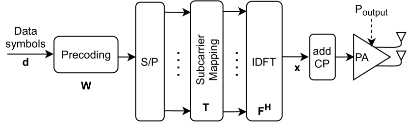
Figure 1: Digital base-band transmitter structure of CP-OFDM.

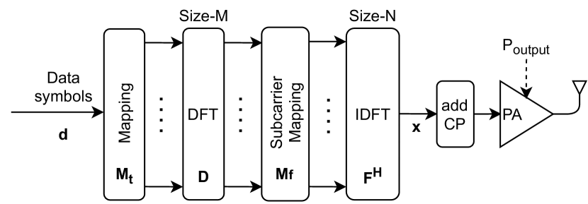
Figure 2: Digital base-band transmitter structure of DFT-S-OFDM.

Regarding the DFT-S-OFDM signal generation (Fig. 2), data symbols are mapped onto a DFT matrix denoted by $\mathbf{D}\in\mathbb{C}^{M\times M}$ via a mapping matrix $\mathbf{M_{t}}\in\mathbb{C}^{M\times N_{d}}$, where $M$ is the DFT size. Then, the output of the DFT is mapped onto a set of subcarriers in the frequency domain through another mapping matrix $\mathbf{M_{f}}\in\mathbb{C}^{N\times M}$. Finally, the output of the matrix $\mathbf{M_{f}}$ is converted to time domain via $\mathbf{F}^{H}$, where $\mathbf{F}^{H}\in\mathbb{C}^{N\times N}$ is the IDFT matrix and $N$ is the number of subcarriers. The final signal $\mathbf{x}\in\mathbb{C}^{N\times 1}$ in the time domain is generated as follows: $\mathbf{x}=\mathbf{F}^{H}\mathbf{M_{f}D_{t}M_{t}d}$. Then, a CP is added to the resulting time signal before being fed into the non-linear PA.

In both cases, output signals are amplified by a non-linear PA, which is assumed to be memory-less with amplitude-to-amplitude distortion only. In particular, a Rapp model is considered [9], whose amplitude-to-amplitude conversion function is given by:

$$g(v,A)=vA\left({1+{\rm{abs}}\left({\frac{{vA}}{{A_{{\rm{sat}}}}}}\right)^{2p}}\right)^{\frac{{-1}}{{2p}}},$$ (1)

where $v$ is the gain of the small-signal, $A$ is the amplitude of the input signal, $A_{\rm sat}$ is the limiting output amplitude, and $p$ controls the smoothness of the transition from the linear region to the saturation regime.

A closed-loop power control mechanism is used in the UL [10], which considers that the BS decides a transmit power, $P_{\rm tx}$, to compensate for the path loss, $\mathrm{PL}$. This transmit power can be expressed in decibels as $P_{\rm tx}=P_{0}+\alpha\mathrm{PL}$ dB, being $P_{0}$ a target received power at the BS, and $\alpha\in[0,1]$ the fractional compensation factor. An Urban Macro (UMa) model has been considered for computing the path loss component, PL.

Restrictions on the maximum transmit power supported by the UE and also out-of-band emissions, impose further limits on the transmitted power. The maximum power reduction (MPR) [1] specifies the decrease in the maximum power transmitted in order to enable the device to fulfill the requirements of the transmitter adjacent channel leakage ratio. This value imposes a maximum transmit power to guarantee that the out-of-band emission is below a given threshold. Since these out-of-band emissions depend on the waveform, modulation level and channel bandwidth, the possible MPR values also depend on such parameters. Finally, the final power transmitted by the UE, $P_{\mathrm{output}}$, can be defined as $P_{\rm output}=\min(P_{\rm decided},P_{\rm max}^{{}^{\prime}})$, where $P_{\rm max}^{{}^{\prime}}=P_{\rm max}-\mathrm{MPR}$.

The SNR is computed as follows:

$$\mathrm{SNR}=P_{\rm output}-\mathrm{PL}+10\,\text{log}_{10}\left(\sum_{i=1}^{N_{\mathrm{rx}}}|h_{i}|^{2}\right)-N_{0}\quad\mathrm{[dB]},$$ (2)

where $N_{\mathrm{rx}}$ is the number of receiver antennas, and $h_{i}$ is the effective channel of the $i$-th receiver antenna after precoding (in case of CP-OFDM). The term $N_{0}$ represents the thermal noise in the band assigned to the user, given by $N_{0}=-204+10\,\text{log}_{10}\left(12\times\Delta f\times N_{\rm RB}\right)+N_{\rm fig}\quad\mathrm{[dBW]}$, where $\Delta f$ is the subcarrier spacing in Hz, $N_{\rm RB}$ is the number of physical resource blocks (PRBs) assigned to the user and $N_{\rm fig}$ is the noise figure at the BS.

III Dynamic Port and Waveform Switching

DPWS feature is targeted to switch between CP-OFDM and DFT-S-OFDM to enhance the UL coverage. In order to achieve that, it uses the following parameters:

• Threshold ($\zeta$): it determines switching occasions from CP-OFDM to DFT-S-OFDM when the following inequality is fulfilled $\mathrm{SNR}<\zeta$.

• Hysteresis ($\xi$): it determines the switching occasions from DFT-S-OFDM to CP-OFDM as follows $\mathrm{SNR}>\zeta+\xi$.

• Counter ($C$): it counts for the number of switching occasions in order to trigger a waveform switching.

• Timer ($T$): it determines the time window to account for switching occasions. To trigger a waveform switch the number of switching occasions must be equal to $C$ within a time window that is smaller than $T$. This time window is expressed as a number of SRS receptions.

The switching mechanism also takes into consideration the SNR estimated with the SRS $(\gamma)$ and the current waveform, as follows. If the transmission is done with CP-OFDM, then a switching occasion is counted if the SNR falls below $\zeta$. However, if the transmission is done with DFT-S-OFDM, then a switching occasion is counted if the SNR raises above $\zeta+\xi$. The switching mechanism is detailed in Algorithm 1, which is executed for each SRS reception.

Input: $\zeta$, $\xi$, C, T, $\gamma$, CurrentWaveform
Initialize: $c=0$, $t=0$

1:  if ($t<T$) then

2:     if CurrentWaveform == CP-OFDM and $\gamma<\zeta$  then

3:        $c=c+1$

4:     else if  CurrentWaveform == DFT-S-OFDM and $\gamma>\zeta+\xi$  then

5:        $c=c+1$

6:     else

7:        $c=0,\,t=0$

8:     end if

9:     if $c\geq{C}$  then

10:        Perform waveform and port switching

11:     end if

12:     $t=t+1$

13:  else

14:     $c=0,\,t=0$

15:  end if

Algorithm 1 DPWS algorithm

The waveform switch is signaled via an RRC reconfiguration message, that changes the UL waveform from CP-OFDM to DFT-S-OFDM and vice-versa. Since the RRC reconfiguration message can change any parameter of the UL transmission, the 3GPP specifications reserve a guard time that allows the UE to prepare for transmission according to the new configuration. According to [10], this guard time depends on the numerology, $\mu$, and on the UE category, but it ranges from $16.75$ ms ($\mu=3$, type 1 category) to $19$ ms ($\mu=0$, type 2 category). Therefore, each switch has a cost in performance since it involves an interruption in the UL transmission, which must be considered by the agent.

IV Proposed Deep Reinforcement Learning Dynamic Switching

Our proposed framework, AI-DWPS, is based on a DRL algorithm. In particular, a Deep Q-Learning (DQL) approach is used, where the Q-Table typically used in classical RL algorithms is substituted by a neural network called Q-Network. This Q-Network is implemented by a Multi-Layer Perceptron (MLP) with a number of nodes in the input layer that matches the cardinality of the state space whereas the number of nodes in the output layer matches the cardinality of the action space. It has a single hidden layer with $n_{\mathrm{hidden}}$ nodes.

In this paper, we propose to optimize the most important DPWS parameters, namely SNR threshold ($\zeta$) and SNR hysteresis ($\xi$). These parameters are controlled by a DRL agent, that can decide to modify them. The DPWS configuration of each cell can be changed based on the actions suggested by the DRL agent. The DRL is located in a central network element, e.g., operations support systems (OSS), or in an external server.

IV-A States, actions, and reward

IV-A1 States

Given the nature of the problem, we have chosen to report statistics about two realistic uplink measurements available in actual networks: the SNR and the TA distrubutions. The throughput metric is defined as the rate of correctly decoded bits per second, whereas the TA indicates how distant is the UE from the serving BS. Both SNR and TA metrics are not reported on a per-connection (i.e., per-user) basis but as a histogram of all connections in a given time window. We have considered $L=12$ bins for TA and SNR. The SNR histogram has the following bins’ limits (in dB): $[-\infty,-5,-2,1,4,7,10,13,16,19,22,25,\infty]$; whereas, the bins’ limits for the TA histogram are (in $\%$): $[5,15,25,35,45,55,65,75,85,95,105,115,\infty]$. Note that the TA bins’ limits are expressed in terms of percentages, being $100\%$ the TA associated with the propagation delay at the maximum range of the cell. This cell range is a network parameter representing the maximum distance (in meters) at which a given BS provides coverage. Due to the channel delay spread, the instantaneous measurement of the TA may provide a value above $100\%$ for cell edge users.

To compress the information given by these histograms we define the following descriptors for the TA and SNR metrics:

$$R_{\ell,{\Psi}}=\frac{\sum_{i=\ell}^{L}\mathrm{BINS}_{i,{\Psi}}}{\sum_{i=1}^{\ell-1}\mathrm{BINS}_{i,{\Psi}}},\;D_{\ell,{\Psi}}=\frac{\sum_{i=\ell}^{L}\mathrm{BINS}_{i,{\Psi}}}{\sum_{i=1}^{\max}\mathrm{BINS}_{i,{\Psi}}},$$ (3)

where $\Psi$ stands for a given metric, i.e., either the SNR or TA, $L$ is the number of bins, and $\mathrm{BINS}_{i,{\Psi}}$ stands for the number of UEs whose metric (TA or SNR) falls within the $i$-th bin interval, which is expressed as $\left[\psi^{-}_{i},\psi^{+}_{i}\right]$.

These metrics inform about the SNR and TA histograms while giving information about their shapes. More specifically, $D_{\ell,\mathrm{metric}}$ represents an estimation of the complementary CDF (CCDF), which represents the probability that the random metric, $\Psi$, is higher than the smaller limit of the $\ell$-th bin, i.e., $\hat{\Pr}(\Psi>\psi_{\ell}^{-})$. Thus, for instance, a value of $D_{9,\mathrm{TA}}\simeq 1$ indicates that almost all UEs in the cell are positioned in the cell edge. On the other hand, $R_{\ell,\mathrm{metric}}$, can be understood as the ratio between the number of occurrences of the random metric being above the smaller edge of the $\ell$-th bin, $\psi_{\ell}^{-}$, and the number of occurrences below such edge of the $\ell$-th bin. Therefore this statistics can be understood as an estimation of this quotient of probabilities, $\hat{\Pr}\left(\Psi\geq\psi_{\ell}^{-}\right)/\hat{\Pr}\left(\Psi<\psi_{\ell}^{-}\right)$.

Let $\mathcal{S}$ be the state space, with $s[n]\in\mathcal{S}$ the instantaneous state at step $n$. The instantaneous state for the DLR algorithm is defined as:

$$s[n]=\{ \zeta[n],\xi[n],\bar{\gamma}[n],R_{6,\mathrm{SNR}},R_{5,\mathrm{SNR}},R_{6,\mathrm{TA}},R_{3,\mathrm{TA}},D_{5,\mathrm{SNR}}\},$$ (4)

being $\bar{\gamma}$ the average SNR across the cell’s UEs and slots related to a given step, $\zeta[n]$ the SNR threshold at step $n$ and $\xi$ the SNR hysteresis at step $n$.

IV-A2 Actions

Let $\mathcal{A}$ be the action space, with $a[n]\in\mathcal{A}$ being the action chosen by the agent at step $n$. The action defines the decision made for each optimizable parameter: SNR threshold $(\zeta)$ and SNR hysteresis $(\xi)$. Both parameters are subjected to 3 possible options: i) decrease the value of the parameter by a certain step, ii) keep the existing value, or iii) increase value by the same step. The decrease/increase step is fixed to $\Delta\zeta=1$ dB and $\Delta\xi=0.5$ dB. $\mathcal{A}$ is therefore comprised of 9 possible actions. Notice that the use of small changes of $\zeta$ and $\xi$ reduces the impact of wrong decisions made by the agent, and allows to reach smoothly optimal values through several iterations.

IV-A3 Reward

To accurately capture the performance of the users in the cell, the reward function is composed of a set of $K$ reward factors, $G_{k},k\in[1,K]\subset\mathbb{N}$, each one corresponding to a certain percentile, $p_{k}$, of the throughput of the cell.

The reward function at step $n$ is given by

$$r[n] =\theta\cdot\mathbf{B}\cdot\left(\Delta G_{1},\Delta G_{2},...,\Delta G_{k}\right)^{t},$$ (5)

$$\Delta G_{k} =\frac{G_{k}[n]-G_{k}[n-1]}{G_{k}[n-1]},$$ (6)

where $\Delta G_{k}$ represents the relative gain of the reward factor $k$ in the cell, $\mathbf{B}=\left(B_{1},..,B_{K}\right)$ is the vector of weights with length $K$ and $\theta$ is a scale factor meant to expand the value range of the reward to help with training. Additionally, to help stabilize the training, the reward peak values are limited by the factor $r_{\mathrm{clip}}$ as follows:

$$r[n]=\mathrm{max}(\mathrm{min}(-|r_{\mathrm{clip}}|,r[n]),\lvert r_{\mathrm{clip}}\rvert).$$ (7)

V Simulation results

The environment has been simulated using the 5G toolbox of MATLAB, whereas the DRL agent has been implemented in Keras & Tensorflow. The detailed parameters of the DRL training are summarized in Table I. During the length of the transmission, the UEs are bounded to the DPWS following the procedure described in Algorithm 1 according to the values of $\zeta$ and $\xi$ of the step. UEs are also subjected to adaptive modulation and coding (AMC), therefore the employed MCS is susceptible to change as the SNR evolves. At any given slot, UEs reporting SNR values below the threshold of the lowest MCS will fall into outage. UEs resulting in outage for the complete duration of the transmission were not scheduled thus not considered in the derived metrics.

During CP-OFDM tranmissions, the precoding matrix W is selected by the BS from the corresponding codebook according to the SRS signal received in order to maximize the received SNR. RL-related parameters can be found in Table I. All UEs share the same configuration parameters, which are summarized in Table II.

TABLE I: RL parameters setting

Parameter	Value
$[\epsilon_{0},\epsilon_{\mathrm{min}}]$	[1, 0.01]
Learning rate	0.05
Training steps per episode	75
# of training episodes	$43$
Evaluation steps per episode	20
# of evaluation episodes	$16$
UEs per episode	50
$n_{\mathrm{hidden}}$	60
Optimizer	Adam
Discount factor	0.01
Batch size	350
Experience buffer size	750
Default threshold, $\zeta$ (dB)	0
Default hysteresis, $\xi$ (dB)	5
$(\theta,r_{\mathrm{clip}})$	$(50,2)$

TABLE II: Network parameters setting

Parameter	Value
$N$ (RBs)	$20$
Transmission length (slots)	$1000$
Carrier frequency (GHz)	$28$
Subcarrier Spacing (kHz)	$15$
User speed (km/h)	$0.4$ (stationary)
Delay Spread (ns)	$30$
Channel Delay Profile	CDL-A
Pathloss model	Urban Macro
SRS Periodicity (ms)	$2$
Min/max UE to BS distance (m)	$25/300$
$(A_{\mathrm{sat}},p)$	$(24$ dBm, $2)$
$P_{\mathrm{max}}$	$23$ dBm

To accurately capture the performance in the edge cell, the reward includes $K$ reward factors, $G_{k}$, associated with low throughput percentiles. More specifically, we have considered $K=8$ reward factors, where the reward factor $G_{1}$ is associated with the $10\%$ percentile, $G_{2}$ with $15\%$ percentile, and so on up to $G_{8}$ with $45\%$ percentile (see Table III). Some bigger percentiles closer to the median are also included as reward factors to avoid harming the average throughput excessively. It was observed during training that relative gains in the lower percentiles were disproportionately bigger compared to those closer to the median. The use of bigger weights for bigger percentiles in the reward function prevents the agent from excessively favoring the lower percentiles and damaging the average cell throughput in the process. Table III summarizes all selected reward factors $G_{k}$ and their associated weights $B_{k}$.

TABLE III: Reward factors and their corresponding weights

$G_{k}$	p10	p15	p20	p25	p30	p35	p40	p45	Avg
$B_{k}$	0.02	0.04	0.06	0.08	0.10	0.12	0.14	0.16	0.18

After the training stage was completed, the agent was evaluated on 16 different episodes. Given the incremental nature of the action space, the agent was given $20$ steps to reach the solution for each episode. It is worth noting that while the UEs in the evaluation stage are drawn from the same configuration as the training stage, the drops, and therefore their positions and channel realizations, are completely independent.

Table IV summarizes the achieved throughput gains of the AI-DPWS waveform switching in contrast to fixed waveform schemes. Throughput gains are expressed in relative and absolute terms for all reward factors $G_{k}$. These results are drawn from the cumulative metrics of all UEs in the 16 evaluation episodes. From the presented table it is easy to observe that the proposed scheme is able to achieve higher throughput for almost all the different reward factors across both fixed waveform schemes. It is worth noting that the bigger relative performance gains are observed towards the lower percentiles even if the absolute gains of all reward factors are comparable. Interestingly, these gains in the lower percentiles do not come as a performance loss in the average throughput of the cell.

TABLE IV: Evaluation results

	Mean throughput gain over:
	CP-OFDM		DFT-S-OFDM
$G_{k}$	%	Abs (Mbps)	%	Abs (Mbps)
p10	297.9299	0.0049	216.8994	0.0046
p15	42.393	0.0159	-16.6991	-0.0125
p20	27.2969	0.0129	7.5623	0.0086
p25	7.9753	0.0122	10.9392	0.0173
p30	8.7799	0.0129	2.0228	0.0046
p35	3.6767	0.0048	3.1608	0.0198
p40	2.3618	0.0067	4.9113	0.0311
p45	-0.2176	-0.0028	6.4336	0.0584
Avg	0.116	0.002	3.3794	0.0603

Finally, to better visualize the impact of AI-DPWS across all UEs in the cell, Fig. 3 (a) and (b) illustrate the achieved throughput of both fixed waveforms and AI-DPWS for low and high throughput percentiles respectively.

As expected, for the lower percentiles, i.e., the cell-edge UEs, DFT-S-OFDM outperforms CP-OFDM. However, AI-DPWS outperforms DFT-S-OFDM by taking into account the conditions of the channel and switching the waveforms accordingly. For higher percentiles, i.e. cell-interior UEs, CP-OFDM outperforms DFT-S-OFDM and in this case, AI-DPWS can only match the performance of the best fixed waveform scheme.

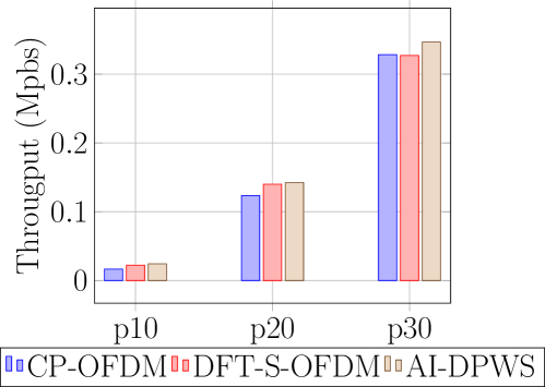
(a)

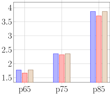
(b)

Figure 3: Achieved throughput with both fixed waveforms and with AI-assisted switching for: (a) low percentiles; and (b) high percentiles.

VI Conclusions

In this paper, a DRL-based framework is proposed to dynamically select the optimal threshold and hysteresis for UL waveform selection based on the DPWS scheme. By using a realistic 5G simulator and realistic measurements available in current networks, it is shown that the proposed scheme outperforms fixed schemes where the waveforms are selected in a static manner. Such performance improvements are exhibited across a wide range of throughput percentiles, showing bigger gains in the lower percentiles, which accounts for the cell-edge UEs. These improvements come without any harm to the average or even top-performing UEs in the cell.

References

- [1] 3GPP, User Equipment (UE) radio transmission and reception; Part 2: Range 2 Standalone (Release 17), 3rd Generation Partnership Project (3GPP) TS 38.101-2, Rev. 17.9.0, April 2023.
- [2] K. Zheng and et al., “Impacts of amplifier nonlinearities on uplink performance in 3g lte systems,” in 2009 Fourth International Conference on Communications and Networking in China, 2009.
- [3] R. Ramirez-Gutierrez and A. Nader, “Switching waveforms for uplink transmission in nr network,” Mar 2021, patent number US2022376965A1.
- [4] A. Feriani and E. Hossain, “Single and multi-agent deep reinforcement learning for ai-enabled wireless networks: A tutorial,” IEEE Communications Surveys & Tutorials, vol. 23, no. 2, pp. 1226–1252, 2021.
- [5] W. Ahsan and et al., “Resource allocation in uplink noma-iot networks: A reinforcement-learning approach,” IEEE Trans. on Wireless Comm., vol. 20, no. 8, 2021.
- [6] N. Costa and et al., “Uplink power control framework based on reinforcement learning for 5g networks,” IEEE Trans. on Vehicular Technology, vol. 70, no. 6, 2021.
- [7] Y. Teng and et al., “Distributed learning solution for uplink traffic control in energy harvesting massive machine-type communications,” IEEE Wireless Communications Letters, vol. 9, no. 4, 2020.
- [8] A. A. Zaidi and et al., “A preliminary study on waveform candidates for 5G mobile radio communications above 6 GHz,” in 2016 IEEE 83rd Vehicular Technology Conference (VTC Spring), 2016.
- [9] C. Rapp, “Effects of HPA-nonlinearity on a 4-DPSK/OFDM-signal for a digital sound broadcasting signal,” in ESA Special Publication, ser. ESA Special Publication, B. Kaldeich, Ed., vol. 332, Oct. 1991, pp. 179–184.
- [10] 3GPP, Technical Specification Group Radio Access Network; NR; Radio Resource Control (RRC) protocol specification (Release 17), 3rd Generation Partnership Project (3GPP) TS 38.331, Rev. 17.4.0, May 2023.