Entangled Matter-waves for Quantum Enhanced Sensing
John Drew Wilson
0000-0001-6334-2460JILA, NIST, and Department of Physics, University of Colorado, 440 UCB, Boulder, CO 80309, USA
Jarrod T. Reilly
0000-0001-5410-089XJILA, NIST, and Department of Physics, University of Colorado, 440 UCB, Boulder, CO 80309, USA
Haoqing Zhang
0000-0002-2481-2412JILA, NIST, and Department of Physics, University of Colorado, 440 UCB, Boulder, CO 80309, USA
Center for Theory of Quantum Matter, University of Colorado, Boulder, CO 80309, USA
Chengyi Luo
0000-0002-9470-5815JILA, NIST, and Department of Physics, University of Colorado, 440 UCB, Boulder, CO 80309, USA
Anjun Chu
0000-0001-8489-9831JILA, NIST, and Department of Physics, University of Colorado, 440 UCB, Boulder, CO 80309, USA
Center for Theory of Quantum Matter, University of Colorado, Boulder, CO 80309, USA
James K. Thompson
0000-0003-1160-5112JILA, NIST, and Department of Physics, University of Colorado, 440 UCB, Boulder, CO 80309, USA
Ana Maria Rey
0000-0001-7176-9413JILA, NIST, and Department of Physics, University of Colorado, 440 UCB, Boulder, CO 80309, USA
Center for Theory of Quantum Matter, University of Colorado, Boulder, CO 80309, USA
Murray J. Holland
0000-0002-3778-1352JILA, NIST, and Department of Physics, University of Colorado, 440 UCB, Boulder, CO 80309, USA
Abstract
The ability to create and harness entanglement is crucial to the fields of quantum sensing and simulation, and ultracold atom-cavity systems offer pristine platforms for this undertaking.
Recently, an experiment demonstrated an effective momentum-exchange interaction between atoms in a common cavity mode [1].
Here, we derive this interaction from a general atom-cavity model, and discuss the role of the cavity frequency shift in response to atomic motion.
We show the cavity response leads to many different squeezing interactions between the atomic momentum states.
Furthermore, when the atoms form a density grating, the collective motion leads to one-axis twisting, a many-body energy gap, and metrologically useful entanglement even in the presence of noise.
This system offers a highly tunable, many-body quantum sensor and simulator.
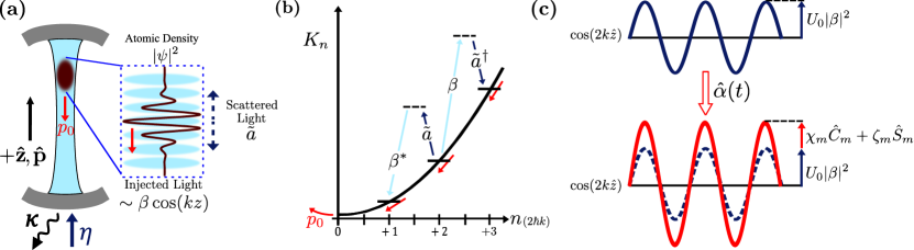
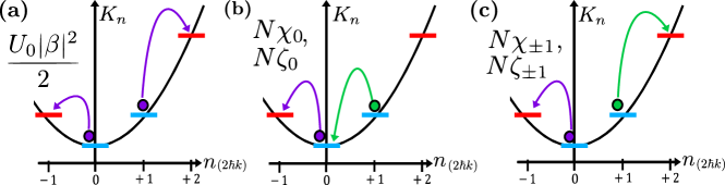
Figure 1:
Experimental scheme for direct generation of entanglement in momentum degrees of freedom for a matterwave interferometer.
(a) The atoms are well confined radially and allowed to move along with a mean momentum of .
The cavity is pumped by a coherent drive such that photons enter the cavity at a rate and leak out at rate .
In the experiment in Ref. [1], a Bragg pulse is applied to prepare into a collective density grating, shown schematically in the inset.
(b) The quadratic kinetic energy spectrum for momentum labeled by , for , and two example interactions with cavity photons in the displaced picture.
Two example processes are shown.
Each transition labeled by the corresponding coherent field (or scattered photon) response for absorption of a photon, (), and for emission, ().
These processes act as a pump for the scattered photons.
(c) The effects of the scattered photons on the atoms.
Where the atoms previously felt a standing field of strength , they now feel a standing field dependent on all other atomic momentum of strength .
For the past century, our ever-growing understanding and control of quantum mechanics has changed the way we design crucial technologies such as atomic clocks [2, 3], biosensors [4], and inertial sensors [5, 6, 7].
These technologies have, in turn, set the stage for major advances in science, allowing for quantum mechanical tests of general relativity [8] and direct observation of gravitational waves [9, 10, 11, 12].
In recent decades, it has been realized that the laws of quantum mechanics fundamentally constrain the levels of precision achievable in experiments on all scales [13], but also that these same laws may be used to benefit sensing experiments [14, 15, 16, 9, 17].
In particular, experiments have demonstrated growing mastery over entanglement as a resource for precision measurement platforms [18, 10, 19, 20] and quantum simulation [21, 22, 23, 24].
A foundational method to generate useful entanglement is that of spin squeezing [17] where atom-atom correlations decrease uncertainty in one phase quadrature by increasing noise in an orthogonal quadrature [16].
This allows sensing protocols to surpass the standard quantum limit (SQL) dictated by wavefunction collapse of unentangled particles, which bounds the uncertainty of an inferred parameter to for constituent particles.
Spin squeezing is primarily done using fine or hyperfine states of atoms [25, 26, 27], which require internal level dynamics to play a major role.
Oftentimes, this means one must transfer the entanglement to another degree of freedom prior to sensing.
This is often the case for atomic clocks [17] where one requires an optical clock transition, and in gravity gradiometry where one requires spatial or kinetic separation.
If one could directly create entanglement among matter-waves similar to a spin-squeezing process, it would create the opportunity for measurements of gravitational effects through matter-wave interferometry with a true quantum advantage.
So far however, generating entangled matter-waves has always involved atomic internal levels as a proxy for the necessary dynamics [19, 20].
Past theoretical works have suggested a myriad of techniques to couple spin squeezing dynamics to the momentum states, such as through the recoil due to absorption and emission of photons [28, 29], two counter-propagating modes of a ring cavity [30], or by using conditional measurements on electronic states to replicate spin squeezing on momentum states in a ring cavity [31].
Recently, an experiment demonstrated One-Axis Twisting (OAT) dynamics between momentum states only through cavity mediated exchange interactions [1].
In this work, we provide a more detailed derivation of this interaction, and carefully discuss the role of the cavity response to atomic motion.
The cavity response to atomic motion is reflected back on the atoms as a dipole force, thereby allowing atoms to self-interact.
This creates the possibility for a different paradigm of entanglement enhanced matter-waves.
Furthermore, when the atoms form a density grating, and their collective motion leads to a pseudo-spin exchange interaction that may be used to realize OAT dynamics and a many-body energy gap.
We show that, in the proper limits, these exchange interactions generate metrologically useful entanglement which could be used to surpass the SQL.
Notably, entanglement is generated between solely the momentum degrees of freedom, which differs from previous works [19, 28, 29, 31, 32, 33].
Self-Interaction via Cavity Frequency Modulation. —
In order to study the effects that drive entanglement, we consider an atomic cloud inside an optical cavity with one relevant mode, as shown in Fig. 1(a).
There are of mass and two relevant internal states, labeled and for the excited and ground states respectively, that are separated by an optical frequency .
The atoms travel along the cavity with mean momentum .
The cavity mode has frequency , which is far detuned from the atomic transition.
The cavity mode has a wavenumber and the atoms have a recoil frequency of due to absorption and emission of cavity photons.
At the anti-node, the atoms have a maximum coupling of to the cavity.
The cavity is pumped by a coherent laser with amplitude and frequency , which is also far detuned from the atomic transition.
The cavity decays at rate , while the atoms spontaneously emit light into free space at a rate .
The system’s density matrix evolves under the Born-Markov master equation,
(1)
where is the system Hamiltonian, is the commutator, the Lindbladian superoperator is given by summed over all jump operators .
Prior to any simplifications, the Hamiltonian is given by the Tavis-Cummings model [34, 35] with a cosine spatial dependence.
The full Hamiltonian and and jump operators for this system are shown in the Supplemental Material (SM) [36].
To recover momentum-only dynamics, we use the fact that the cavity photon frequency and the laser pump frequency are both far detuned from the atomic transition frequency, such that , with being the pump detuning from the atomic transition frequency.
This allows us to adiabatically eliminate the excited state [36].
After elimination, the atom-field Hamiltonian is
(2)
where () is the vertical momentum (position) operator for atom parallel to the cavity axis, is the pump detuning from the dressed cavity photon frequency, and is the effective coupling strength.
Photon leakage from the cavity leads to a jump operator , and spontaneous emission from atom leads to , where is the operator representing the atomic recoil following the dipole radiation pattern , for being the angle between the emitted photon and the positive -axis [37, 38].
The spontaneous emission is now understood as a photon initially being absorbed from the cavity field through at rate , and subsequently emitted through at rate .
The relevant physical mechanism that leads to entanglement is the spatially dependent frequency shift on the cavity induced by the atomic motion.
To illuminate this effect, we consider the displaced reference frame of the cavity field, with , where is the coherent field injected by the pump and is the annihilation operator on the scattered photon field.
The atom-cavity Hamiltonian in this reference frame is
(3)
Now, the spatially dependent frequency shift explicitly shows up in the scattered photons through the first term in the second line of Eq. (3).
This process may be equivalently understood through the two-photon absorption and emission process, shown in Fig.1(b).
The scattered photon have a new frequency corresponding to the Doppler shift of the atomic motion.
In Ref. [1], two momentum states were considered via a pseudo-spin mapping.
Here, we consider a generalized treatment of all momentum states through a second quantization approach in the momentum basis [36].
Later, we will restrict to only two momentum states to find the effective OAT interaction and momentum-exchange.
We label momentum states by integer multiples, for integer , where the annihilation (creation) operator for an atom in the state is ().
This requires that the atoms initially have a narrow spread in momentum about [36] less than one .
This allows us to define the quadratic raising and lowering operators , so that .
Additionally, we define and so that and .
This means , where is the kinetic energy for the momentum state and is the mean momentum state such that .
We integrate out the cavity response [36] following Ref. [39] based on assumptions of a small coupling, .
This is equivalent to solving the equations of motion for in the displaced reference frame, where the scattered photons adiabatically follow the atomic motion.
This yields the effective replacement where is an atomic operator defined as
(4)
where the amplitude depends on the required change in kinetic energy due to the two photon transition.
This yields a Hamiltonian that only involves momentum degrees of freedom
(5)
where
(6)
are the rates for the cosine and sine non-linear interactions, with and being the real and imaginary parts of , respectively.
The jump operators in this framework are given by the same collective atomic recoil due to cavity decay, now , and a single atomic recoil term, which is not simply expressed in the second quantization approach, but is treated explicitly in the SM [36].
The two decay processes are understood simply as follows: the collective atomic recoil occurs when a photon entangled to the atomic motion is lost out of the cavity, through with rate . The individual atomic recoil, meanwhile, occurs when an atom directly scatters a photon from the coherent field, at rate , out of the cavity at angle , at rate .
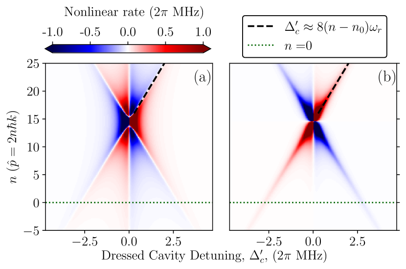
Figure 2:
(a) for all momentum states .
(b) for all momentum states .
For both plots, sets the resonance.
The black dashed line represents one of the resonances in for .
There is a corresonding line of negative slope for the other resonance, not explicitly labeled.
The green dotted line for , denotes the rate , matching the one for the momentum states prepared in Ref. [1].
The cut off of MHz was chosen to show contrast near , but not cut off the features near .
The two non-linear terms, and , generate a type of generalized squeezing dynamics [40].
The cosine-cosine non-linearity, , is the modification of the optical lattice due to scattered photons.
The sine-cosine non-linearity, , is due to the fact that the scattered photons cause the cosine and sine quadrature to no-longer be perfectly orthogonal, and we note is nearly zero unless near a resonance in .
As a function of momentum and pump detuning from the dressed cavity photon frequency, the two rates and are shown in Fig. 2 with the physical parameters given in the SM [36], where one of the two resonances is shown as a black dashed line.
In the rest of this paper we study the entanglement generation in a simple regime of Eq. (5), where we restrict to only two momentum states.
There, the non-linear interactions in Eq. (5) yield OAT dynamics on the two-level manifold, which we show leads to an effective momentum exchange [1] and metrologically useful entanglement.
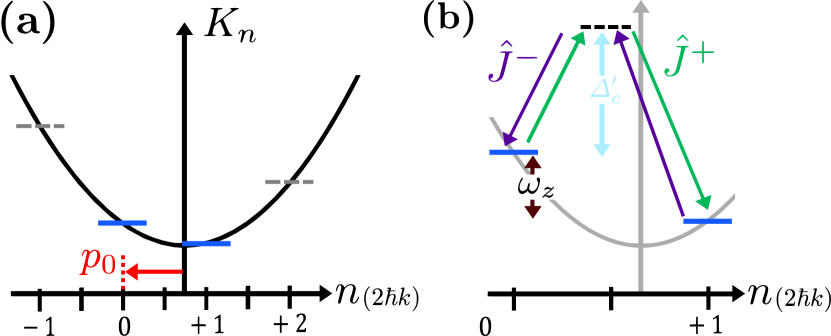
Formation of a Density Grating. —
When the atoms occupy just the two momentum states, and . they form a density grating.
This may be achieved physically by selecting an appropriate and applying a Bragg pulse, such as is done in Ref. [1].
The choice of translates the kinetic energy spectrum in momentum, shown in Fig. 3 (a), thereby allowing the momentum states and to be addressed independently by tuning the dressed cavity-pump detuning, , as is shown in Fig. 3 (b).
By restricting to these two-levels, we are left with only two-level operators shown schematically in Fig. 3 (b).
For brevity, we drop the subscripts; and , and .
These two momentum states are separated by a kinetic energy .
The interference pattern of the two momentum states forms a density grating composed of all atoms.
The motion of this density grating modifies the dressed cavity frequency, and drives scattered photons according to
,
with the now collective amplitudes .
These substitutions give a typical OAT Hamiltonian;
(7)
where and have taken the place of cosine and sine, respectively.
For clarity, non-linear rates on this two-level manifold simplify to
and
.
Notably, is the same as the spin exchange rate given in Ref. [1], and matches the slice at of Fig. 2 (a).
The two non-linearities in Eq. (7) arise from the cosine-cosine and cosine-sine modulation in Eq. (5), where now the motion of the atomic ensemble acts in unison rather than in many different momentum states, leading to an effective collective enhancement of on the non-linear rates.
With these rates defined, we now discuss the conditions for energetically isolating these two momentum states from the rest of the momentum basis.
We require that higher momentum states aren’t excited via either Bragg scattering off the coherent field, , or non-linear interactions, in Eq. (5).
These restrictions ensure the dynamics remain in the two-level manifold, and give limits on the rates , and , in Eq. (7);
(8)
The explicit calculation of these is given in the SM [36], and it is important to note that the inequalities in Eq. (8) only guarantees unitary dynamics won’t drive higher momentum states– quantum jumps may still drive higher momentum states.
The first of these terms is the condition that the atoms are well into the conduction band of the optical lattice–meaning they translate smoothly over the lattice.
The second term is the condition that the nonlinear effects aren’t driven so strongly that they couple to higher momentum states.
Figure 3:
(a) The kinetic energy spectrum, with the translation due to shown in red.
(b) The kinetic energy spectrum zoomed in to only show the two-level approximation.
Here, we’ve shown .
In the two-level approximation, the effects of the pseudo-spin raising (green) and lowering (purple) operators are shown with energy between and , and the meta-state (dotted line) with the energy of a dressed cavity photon, .
Lastly, we consider the regime where the atoms are fast moving, or the pump is far detuned from the cavity.
In Fig. 2 we see that either of these conditions, large or large , will yield a small and .
Here, becomes large compared to all other frequencies, such as , , and .
We take an interaction picture with and drop terms which are fast rotating.
Mathematically, this is a rotating wave approximation and physically, this means the rate of single atom interactions with the optical lattice is small compared to the kinetic energy.
This means , so we approximate that , and .
Lastly, the decay due to collective emission in the Born Markov master equation splits such that , where and , with .
This regime represents an effective momentum exchange between the atoms, and this interaction drives the effects studied in Ref. [1], where
the Hamiltonian simplifies to
(9)
In this dispersive regime, only the energy conserving interactions of affect the unitary dynamics, where one atom exchanges its momentum state with another via a dispersive cavity photon.
Through this energy conservation, a strong bias appears against effects which would take the atoms out of a symmetric configuration.
This leads to a large many-body energy gap of the form , which is a pseudo-spin length that biases against dynamics between states with different eigenvalues, i.e., between states of different permutational symmetry.
This many-body energy gap leads to a further suppression of single atom effects by slowing down the effective rate of single particle decoherence effects such as Doppler broadening [1, 41].
Spin Squeezing with Decoherence. —
To calculate the usefulness in the presence of noise we consider the atomic species 87Rb, and the initial state (a eigenstate).
We use the numerical parameters given in the SM [36].
Collective emission through the cavity is the biggest barrier to achieving a quantum advantage through this momentum squeezing, unless the pump is far detuned cavity.
In this regime, single particle emission becomes relevant, which causes atoms to be lost from the two-level manifold at a rate
(10)
which is explicitly calculated in the SM [36].
In order to study the generation of entanglement in the presence of decoherence, we calculate the Dicke spin squeezing parameter [42];
(11)
where is the variance, is the pseudo-spin tilted at angle and perpendicular to the average spin length, .
Notably, and therefore, indicates better than SQL certainty and the presence of metrologically useful entanglement [29].
We assume that the squeezing is done for short times, such that , and collective decoherence doesn’t drive atoms out of the two-level manifold.
This assumption allows dissipative dynamics to be treated independently of the OAT dynamics, so we add uncertainty due to collective emission in quadrature to variance of the squeezed state.
We calculate the mean-field dynamics [36], where we find
(12)
where is the contribution due to collective decoherence.
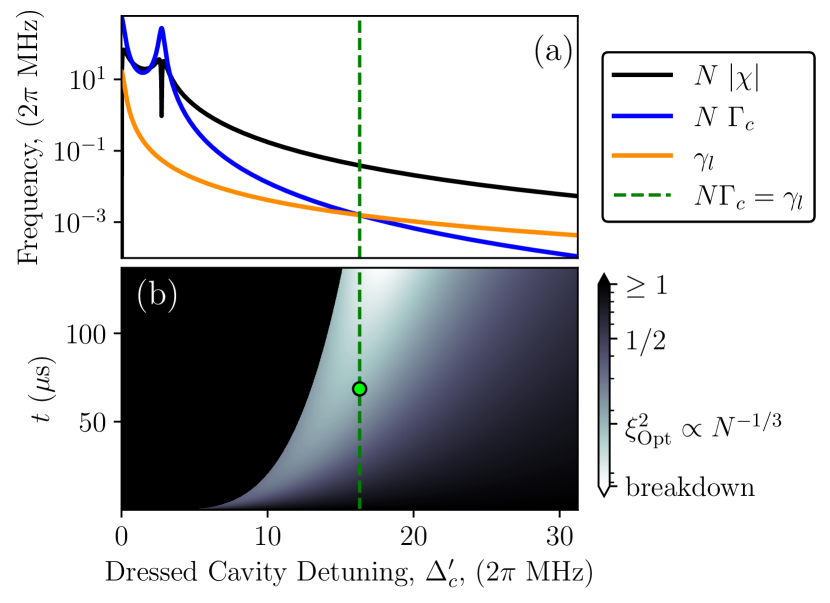
In Fig. 4 (a) we show these four rates, for 87Rb atoms.
The spin squeezing parameter is minimized as a function of squeezing time, , and detuning of the pump from the dressed cavity detuning, .
First, if one tunes the pump laser frequency such that the dressed cavity detuning, , is too near the resonance in , then collective decay dominates, , and we ignore single particle decoherence.
Here, it has been shown [36, 43] that the spin squeezing parameter is limited to at the optimal squeezing time.
This corresponds to , which is proportional to the SQL, at best.
In order to achieve better than SQL sensitivity, we consider the far detuned regime where collective decay is smaller, and single particle effects limit the squeezing time.
By balancing the single particle decoherence and collective decoherence, we find such that , shown in Fig. 4(a) and (b) by the green dashed vertical line.
To highest order in , we find an optimal squeezing time and dressed cavity detuning of
(13)
and an optimal spin squeezed parameter of
(14)
which corresponds to and is better than SQL scaling.
Lastly, if using the fact that , we have , and
(15)
where is an effective single atom co-operativity.
In Fig. 4 (b), we show that for an atomic detuning of MHz, and a pump rate of MHz, the optimally squeezed state is reached in a time of 150 s.
Figure 4:
(a) Collective rates that appear in the optimized spin squeezing parameter.
(b) Eq. (11) as a function of squeezing time, , and Dressed cavity detuning, .
We note that while values of lower than are found, these values are in the regime where the assumption that noise adds in quadrature is close to breaking down, i.e. where the assumptions that , are close to breaking down.
Conclusion. —
In this work, we provided a detailed derivation of the momentum exchange interaction in Ref. [1], and discussed its connection to the frequency shift of an optical cavity mode due to atomic motion.
We have introduced a method which may be used to realize momentum based entanglement independent of electronic degrees of freedom with many possible squeezing interactions, shown in Eq. (5).
These squeezing interactions are generated from the cavity field’s response to the atomic motion.
We showed that, in proper limits, the momentum states may be truncated to form an effective two-level system to the momentum states and , which form a density grating inside the cavity.
Using this effective two-level system, we have demonstrated that entanglement is generated even in the presence of noise.
Here, we’ve limited the discussion of entanglement generation to an effective two-level truncation, but one could go further to realize multi-level squeezing dynamics from Eq. (5).
Of particular interest is the use of these additional states to realize multi-level dynamics via the use of additional dressing lasers to drive higher order interactions.
Furthermore, these momentum states provide a promising opportunity for realizing spin squeezing via two-axis counter twisting effects [44, 45], which can be achieved by periodically modulating the amplitude injected field at a parametric resonance [44] or injecting a second pump [45].
Lastly, future work could include using measurements on the light field exiting the cavity.
This light is highly entangled to the atoms, and measurements would, in principle, allow one to induce a back-action on the atomic cloud.
This creates the opportunity for quantum non-demolition measurements similar to those presented in Ref. [19], or even for extending methods of continuous phase tracking [46] directly to matter-wave interferometry.
Acknowledgments. —
The authors thank Simon B. Jäger, Maya Miklos, Tyler Sterling, and John Cooper for helpful conversations.
This material is based upon work supported by the U.S. Department of Energy, Office of Science, National Quantum Information Science Research Centers, Quantum Systems Accelerator. We acknowledge additional funding support from the National Science Foundation under Grant Numbers PHY 2317149; OMA 2016244; PHY 2317149; PHY 2207963; and 2231377, NIST, and DARPA/ARO W911NF-19-1-0210; and W911NF-16-1-0576, AFOSR grants FA9550-18-1-0319; and FA9550-19-1-0275.
References
Luo et al. [2024a]C. Luo, H. Zhang, V. P. Koh, J. D. Wilson, A. Chu, M. J. Holland, A. M. Rey, and J. K. Thompson, Science 384, 551 (2024a).
Richardson et al. [2020]L. Richardson, A. Hines, A. Schaffer, B. Anderson, and F. Guzmán, Applied Optics 59 (2020).
Templier et al. [2022]S. Templier, P. Cheiney, Q. d’Armagnac de Castanet, B. Gouraud, H. Porte, F. Napolitano, P. Bouyer, B. Battelier, and B. Barrett, Science Advances 8, eadd3854 (2022).
Bothwell et al. [2022]T. Bothwell, C. J. Kennedy, A. Aeppli, D. Kedar, J. M. Robinson, E. Oelker, A. Staron, and J. Ye, Nature 602, 420 (2022).
Aasi et al. [2013]J. Aasi, J. Abadie, B. Abbott, R. Abbott, T. Abbott, M. Abernathy, C. Adams, T. Adams, P. Addesso, R. Adhikari, et al., Nature Photonics 7, 613 (2013).
Pedrozo-Peñafiel et al. [2020a]E. Pedrozo-Peñafiel, S. Colombo, C. Shu, A. F. Adiyatullin, Z. Li, E. Mendez, B. Braverman, A. Kawasaki, D. Akamatsu, Y. Xiao, and V. Vuletic̀, Nature 588, 414–418 (2020a).
Greve et al. [2022]G. P. Greve, C. Luo, B. Wu, and J. K. Thompson, Nature 610, 10.1038/s41586-022-05197-9 (2022).
Malia et al. [2022]B. K. Malia, Y. Wu, J. Martínez-Rincón, and M. A. Kasevich, Nature 612, 661 (2022).
Georgescu et al. [2014]I. M. Georgescu, S. Ashhab, and F. Nori, Reviews of Modern Physics 86, 153 (2014).
Mei et al. [2022]Q.-X. Mei, B.-W. Li, Y.-K. Wu, M.-L. Cai, Y. Wang, L. Yao, Z.-C. Zhou, and L.-M. Duan, Phys. Rev. Lett. 128, 160504 (2022).
Steinert et al. [2023]L.-M. Steinert, P. Osterholz, R. Eberhard, L. Festa, N. Lorenz, Z. Chen, A. Trautmann, and C. Gross, Phys. Rev. Lett. 130, 243001 (2023).
Cao et al. [2023]M.-M. Cao, K. Li, W.-D. Zhao, W.-X. Guo, B.-X. Qi, X.-Y. Chang, Z.-C. Zhou, Y. Xu, and L.-M. Duan, Phys. Rev. Lett. 130, 163001 (2023).
Pedrozo-Peñafiel et al. [2020b]E. Pedrozo-Peñafiel, S. Colombo, C. Shu, A. F. Adiyatullin, Z. Li, E. Mendez, B. Braverman, A. Kawasaki, D. Akamatsu, Y. Xiao, and V. Vuletic̀, Nature 588, 414–418 (2020b).
Norcia et al. [2018]M. A. Norcia, R. J. Lewis-Swan, J. R. Cline, B. Zhu, A. M. Rey, and J. K. Thompson, Science 361, 259 (2018).
Muniz et al. [2020]J. A. Muniz, D. Barberena, R. J. Lewis-Swan, D. J. Young, J. R. Cline, A. M. Rey, and J. K. Thompson, Nature 580, 602 (2020).
Tavis and Cummings [1968]M. Tavis and F. W. Cummings, Physical Review 170, 379 (1968).
Dong et al. [2022]Z. Dong, G. Zhang, A.-G. Wu, and R.-B. Wu, IEEE Transactions on Automatic Control 68, 2048 (2022).
Note [1]See Supplemental Material. Here, we write down the full Hamiltonian from which we start this work, eliminate the excited state, second quantize the momentum degree of freedom, eliminate the cavity, put bounds on the two level approximation, and optimize the spin squeezing parameter through semi-classical treatment.
Bartolotta [2021]J. Bartolotta, Advances in Laser Slowing, Cooling, and Trapping using Narrow Linewidth Optical Transitions, Ph.D. thesis, University of Colorado Boulder, Boulder (2021).
Jäger et al. [2022]S. B. Jäger, T. Schmit, G. Morigi, M. J. Holland, and R. Betzholz, Physical Review Letters 129, 063601 (2022).
The full Hamiltonian and jump operators from the main text is given by
(16)
where () is the photon creation (annihilation) operator of the cavity mode, () is the momentum (position) operator for the th atom parallel to the cavity axis, , are Pauli matrices for the atom, and is the operator representing the atomic recoil following the dipole radiation pattern.
The dipole radiation pattern is calculated by considering a specific dipole radiation pattern.
As an example, in simulations we consider the rubidium dipole allowed transition from to and tracing out the and degrees of freedom [37, 38].
This yields
(17)
where is the angle between the emitted photon and the positive -axis [37, 38].
If we had considered states with another angular momentum difference, this would lead to a different dipole radiation pattern.
The full term in the Lindblad equation is then integrated over :
(18)
A.1 Numerical Simulation Parameters
For the two relevant atomic levels we consider the cycling transition, with a transition wavelength of nm and a decay rate of MHz [47].
The single relevant mode of the cavity couples to the atoms with a single-atom coupling strength of MHz and decays at a rate MHz.
The atom-pump detuning is MHz with a pump coupling rate of MHz, corresponding to the rate at which pump photons make it through the mirror.
The atoms are accelerated to have a mean momentum of , which provides an energy splitting of MHz, which matches Ref. [1] to an order of magnitude.
Appendix B Adiabatic Elimination of the Excited State
From Eq. (16) we transform the system’s original density matrix, into a rotating frame, with the unitary .
We eliminate the excited state based on the assumption , with .
Subject to the above constraints , which is equivalent to solving .
We solve this using the Heisenberg picture of Eq. (16):
(19)
Using yields
(20)
and therefore
(21)
To reconstruct the correct Hamiltonian and jump operators, we consider the time evolution of the cavity operator , and of the momentum operator :
(22)
where includes integration about as in Eq. (18).
We replace with the right hand side of Eq. 21 to find the atom-field Hamiltonian and jump operators
(23)
with being the dressed cavity detuning.
The state is now represented by the density matrix , where is the trace over the atomic degrees of freedom.
Appendix C Discretized Momentum Space
We note that the single particle jump operator does not fit conveniently in this formalism, but later when considering squeezing we treat single particle decoherence explicitly.
The entire Hamiltonian now contains only collective momentum physics, which we second quantize via
(24)
so that each sum over all particles is replaced by an integral over an operator valued measure.
We also impose that , ie there are total atoms.
We additionally assume the particles have near zero-momentum width, so that
(25)
for .
This means that in terms like the kinetic energy.
Going term by term, this yields;
(26)
where is the kinetic energy for the momentum state and is the mean momentum state such that .
Each of the trigonometric operators is simply expressed in this formalism as well;
(27)
which we use to write
(28)
and
(29)
We note that , following from an commutation relation.
This means the Hamiltonian after displacement is
(30)
Appendix D scattered photons in the cavity
Now, we eliminate the cavity scattered photons.
We identify as the momentum only Hamiltonian, and as the fluctuation only Hamiltonian.
To eliminate fluctuations, we use a displacement
(31)
where is a position/momentum operator.
We solve for the equations of motion of following Ref. [39];
(32)
Here, we observe that .
Dropping this term is equivalent to dropping the next order of modulation, i.e. the frequency shift of the quantum degrees of freedom by the atoms.
In other words, we only solve for the central cavity peak interacting with the atoms (first order), the frequency modulation of the central cavity peak (second order), and the interaction of the atoms with that peak (third order), and not the fourth order modulation of these scattered photons–which is the same order as the modulation due to spontaneous emission that we already dropped.
All together, we must solve
(33)
We can make the ansatz that
(34)
where the amplitude carries the time and momentum dependence for photon absorption in the direction, and is the corresponding momentum kick direction in that direction.
We note that
(35)
This ansatz yields two uncoupled differential equations;
(36)
which have solutions
(37)
where we’ve dropped the initial time dependent decay from the pump being turned on.
Now, we note that and substitute this back into the Hamiltonian;
(38)
where we write in the real (hermitian) and imaginary (anti-hermitian) components:
(39)
We also note that .
Therefore
(40)
This yields
(41)
where
(42)
are the rates for the cosine and sine non-linear interactions.
This also yields the collective jump operator
Appendix E Two Level Mapping
Figure 5: (a) Single atom processes which break the two-level assumption, due to Bragg scattering off of the optical lattice.
(b) and (c) Multi-atom process which break the two-level approximation.
(b) An example transition which occurs with rate or , where one atom (purple) leaves the two-level manifold but the other atom (green) does not.
This is the multi-atom process which pre-dominantly breaks the two-level approximation.
(c) An example transition which occurs with rate or , where both atom (purple and green) leave the two-level manifold.
This the multi-atom process has a higher energy barrier than if one atom stayed in the manifold.
Now, we restrict ourselves to just (the and states).
By restricting to these two levels, we are left with only two-level operators;
(43)
These two momentum states are separated by a kinetic energy .
Now, we use the following:
(44)
This means
(45)
where the terms labeled for break the two-level approximation;
(46)
if we only keep the terms that keep us in the two-level manifold we get, and gauge transform away terms proportional to , then we find
(47)
where we drop the subscript in the main text: and .
E.1 Restrictions on the Two-Level Mapping
Separating these two momentum states requires that none of the terms drive atoms out of this two level manifold.
These terms amount to Bragg scattering, , and the nonlinear cosine-cosine and cosine-sine interactions, , , and .
The first term, Bragg scattering, could break the two level approximation by allowing the following single particle transition:
(48)
through the transition elements;
(49)
shown schematically in Fig. 5 (a).
These single particle terms come with the energy condition:
(50)
Using this, we can consider the effective Rabi-oscillation between and or and , which yields the energy condition the maximum probability of excitation [48]:
(51)
for being the smaller of the two energy gaps.
This yields the condition that
(52)
In the limit that that atoms are fast moving, , this yields
(53)
which means that the standing field will also have low probability of driving as well.
The second set of terms, , , and correspond to non-linear interactions.
These drive two atom transitions, such as the two examples in Fig. 5 (b) and (c) and therefore have many more ways to break the two-level approximation.
For two atomic states labeled by the pair with the symmetrizer and momentum states , the transitions which break the two level approximation are
(54)
Each of these have a corresponding matrix element, such as in the case.
However, the transitions and from will always have the lowest energy cost with .
Furthermore, we care about maximizing and to optimize squeezing on this two level manifold, so we only bound these two rates.
In principle, this process provides bounds for every rate appearing in .
This gives:
(55)
So, these two restrictions together are
(56)
E.2 Single Particle Decay
In the two-state approximation for momentum, the spontaneous emission breaks permutational symmetry.
To calculate the final jump operators in the two mode picture, we preemptively define single particle pseudo-spin operators;
(57)
Furthermore, single particle spontaneous emission doesn’t stay on the momentum grid like coherent dynamics or collective decay.
To treat this, we assume that
(58)
for and where and are chosen such that the first and second moments of the momentum-recoil matches the continuous case [38, 37].
With two free variables, and , this is the best we can do.
This yields and , which means the original spontaneous emission operator in Eq. (18) becomes
(59)
where
(60)
After eliminating the excited state we find
(61)
but we assume that spontaneous emission is only due to absorption from the coherent field, so that .
This yields
(62)
which, in the discrete momentum family, becomes
(63)
Here, we note that acting on the state or always leads to atom loss from the 2-level manifold.
, however, does not:
(64)
and, therefore,
(65)
where represents atom loss into states like .
The approximation that an atom in these states is lost is valid for short times because while these states remain relatively un-populated.
Appendix F Optimal Spin Squeezing Parameter
We take the one axis twisting Hamiltonian from the main text, and ignore the many-body energy gap, ;
(66)
where
(67)
for particle loss rate found in Eq. (65).
As an aside, we have assumed that all three decay channels lead to particle loss–which strictly over-estimates the total decay.
The squeezing parameter is given by:
(68)
For short squeezing times the average pseudo-spin is in the -direction, and the length goes as, , for being the total initial pseuo-spin length.
We note that .
The minimum over is the smallest eigenvalue of the covariance matrix;
(69)
for and .
The state is initially polarized in and therefore over short times.
The eigenvalues of C are:
(70)
where
(71)
For short times, the OAT dynamics can be treated independently of collective decay, and fluctuations from collective emission are added in quadrature to the fluctuations due to squeezing.
We first solve for the spin squeezing parameter in the collcetive case, , and then add the effects of collective decay back in by modifying , with an additional term for each collective decay channel:
For intermediate times, we have that , and therefore
(74)
so
(75)
Now, since we are considering short squeezing times we have small , and approximate .
We also use large to drop terms for half or whole small integer .
(76)
We identify as a small unitless parameter and series expand to .
(77)
This all yields
(78)
and
(79)
Now, we collect terms and drop them according to for strongly squeezed quadratures, yielding
(80)
where, because we aren’t near the limit of oversqueezed states, we don’t have the typical curvature term .
Lastly, we add back in the term for collective emission.
In the limit of large , we have that , and therefore
(81)
where is the spin squeezing parameter without collective decay.
This yields
(82)
Where, lastly, we series expand to first order in .
(83)
yielding, as a final expression,
(84)
where is the collective decay defined in the main text.