Inferring kinetics and entropy production from observable transitions in partially accessible, periodically driven Markov networks

Abstract

For a network of discrete states with a periodically driven Markovian dynamics, we develop an inference scheme for an external observer who has access to some transitions. Based on waiting-time distributions between these transitions, the periodic probabilities of states connected by these observed transitions and their time-dependent transition rates can be inferred. Moreover, the smallest number of hidden transitions between accessible ones and some of their transition rates can be extracted. We prove and conjecture lower bounds on the total entropy production for such periodic stationary states. Even though our techniques are based on generalizations of known methods for steady states, we obtain original results for those as well.

1 Introduction

The framework of stochastic thermodynamics provides rules to describe small physical systems that are embedded into a thermal reservoir but remain out of equilibrium due to external driving [1, 2, 3]. If the relevant degreees of freedom can be described by a memoryless, i.e., Markovian dynamics on a discrete set of states, the time-evolution of the system is governed by the network structure and the transition rates between the states. In the case of periodically driven transition rates, such a dynamics relaxes into a periodic stationary state (PSS) [4, 5, 6, 7], which, as a special case, becomes a non-equilibrium steady state (NESS) [8, 9, 10, 11] for constant transition rates.

Since a model is fully specified only if all transition rates are known, practically relevant scenarios in which parts of the model remain hidden [12, 13] require methods to recover, e.g., hidden transition rates on the basis of observable data of a particular form. The combination of such methods with the physical constraints provided by the rules of stochastic thermodynamics comprises the field of thermodynamic inference [14]. With a focus on quantities that have a thermodynamic interpretation, recent works in the field obtain bounds on entropy production [15, 16, 17, 18, 19, 20] or affinities [19, 21, 22, 23], which are complemented with techniques to recover topological information [24, 25] and speed limits [26, 27, 28].

Many of the methods discussed above apply to the case of time-independent driving and cannot straightforwardly be generalized to a PSS. For one of the standard methods of estimating entropy production, the thermodynamic uncertainty relation [29, 30], generalizations to PSSs exist [31, 32, 33, 34], which require more input than their time-independent counterparts in general.

For the purpose of estimating entropy production, the usual rationale if given information about residence in states is to identify appropriate transitions or currents, since such time-antisymmetric data allow one to infer the entropy production. When observing transitions, one can ask the converse question: Can we infer information about states, which are time-symmetric, from antisymmetric data like transitions? We will address in this work how observing transitions allows us to recover occupation probabilites in states if the system is in a PSS. In addition, we will generalize and extend methods from [19] to the periodically driven case to infer transition rates and the number of hidden transitions between two observable ones. We also formulate and compare different lower bounds on the mean total entropy production. These entropy estimators are either proved or supported with strong numerical evidence.

The paper is structured as follows. In Section 2, we describe the setting and identify waiting-time distributions between observed transitions as the basic quantities we use to formulate our results. In Section 3, we investigate how these quantities can be used to infer kinetic information about the hidden part of a system in a PSS or NESS. Estimators for the mean entropy production are discussed in Section 4. We conclude and give an outlook on further work in Section 5.

2 General setup

We consider a network of $N$ states $i\in\left\{1,\dots,N\right\}$ that is periodically driven. The system is in state $i(t)$ at time $t$ and follows a stochastic description by allowing transitions between states sharing an edge in the graph. A transition from $k$ to $l$ happens instantaneously with rate $k_{kl}(t)$, which has the periodicity of the driving. To ensure thermodynamic consistency, we assume the local detailed balance condition [1, 2, 3]

$$\frac{k_{kl}(t)}{k_{lk}(t)}=e^{F_{k}(t)-F_{l}(t)+f_{kl}(t)}$$ (1)

at each link, i.e., for each transition and its reverse. The driving with period $\mathcal{T}$ may change the free energy $F_{k}(t)$ of states $k$ or act as a non-conservative force along transitions from $k$ to $l$ with $f_{kl}(t)=-f_{lk}(t)$. Energies in this work are given in units of thermal energy so that entropy production is dimensionless.

The dynamics of the probability $p_{k}(t)$ to occupy state $k$ at time $t$ obeys the master equation

$$\partial_{t}p_{k}(t)=\sum_{l}\left[-p_{k}(t)k_{kl}(t)+p_{l}(t)k_{lk}(t)\right].$$ (2)

In the long-time limit $t\to\infty$, these networks approach a periodic stationary state (PSS) $p^{\text{pss}}_{k}(t)$. The transition rates and these probabilities $p^{\text{pss}}_{k}(t)$ determine the mean entropy production rate in the PSS [1, 2, 3]

$$\left\langle\sigma\right\rangle_{\text{pss}}\equiv\frac{1}{\mathcal{T}}\int_{0}^{\mathcal{T}}\sum_{kl}p^{\text{pss}}_{k}(t)k_{kl}(t)\ln\frac{p^{\text{pss}}_{k}(t)k_{kl}(t)}{p^{\text{pss}}_{l}(t)k_{lk}(t)}\differential{t}.$$ (3)

In this work, we assume that at least one pair of transitions of a Markov network in its PSS or NESS is observable for an external observer while other transitions and all states are hidden, i.e., not directly accessible for the observer. We illustrate this with graphs of two exemplary Markov networks in Figure 1. States with an observable transition between them will be called boundary states. If two boundary states are connected with one hidden transition, these transitions and the boundary states form the boundary of the hidden network. Additionally, we assume the period $\mathcal{T}$ of the driving to be known.

The task is to determine hidden quantities like the probabilities $p^{\text{pss}}_{k}(t)$ of such partially accessible networks as well as to estimate the overall entropy production.

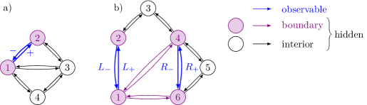
Figure 1: Graphs of partially observable, periodically driven Markov networks. Observable transitions are labeled and displayed in blue. All states and the remaining transitions are assumed to be hidden. Purple states and purple transitions form the boundary of the hidden network. In a), only one pair of transitions can be observed. In b), the two pairs $1\leftrightarrow 2$ and $4\leftrightarrow 6$ are observable. The whole network consists of the observable transitions, the boundary of the hidden network and its interior.

In such a network, we can determine distributions of waiting times $t$ between two successive observable transitions $I=(ij)$ and $J=(kl)$, whereas observing the full microscopic dynamics is impossible. These waiting-time distributions are of the form

$$\psi_{I\to J}(t|t_{0}) \equiv\sum_{\gamma_{I\to J}(t,t_{0})}\mathcal{P}\left[\gamma_{I\to J}(t,t_{0})\middle|I,t_{0}\right].$$ (4)

They depend on the time $t_{0}\in[0,\mathcal{T}]$ at which transition $I$ occurs within one period of the PSS. Since an arbitrary number of hidden transitions occurs between $I$ and $J$, the distributions are given by the sum of conditional path weights $\mathcal{P}\left[\gamma_{I\to J}(t,t_{0})\middle|I,t_{0}\right]$ corresponding to all microscopic trajectories $\gamma_{I\to J}(t,t_{0})$ that start directly after a transition $I$ at $t_{0}$ and end with the next observable transition $J$ after waiting time $t$.

Furthermore, we define

$$\Psi_{I\to J}(t)=\int_{0}^{\mathcal{T}}p^{\text{pss}}(t_{0}|I)\psi_{I\to J}(t|t_{0})\differential{t_{0}},$$ (5)

where we use the conditional probability $p^{\text{pss}}(t_{0}|I)$ to detect a particular transition $I$ at a specific time $t_{0}\in[0,\mathcal{T})$ within the period. Due to effectively marginalizing $t_{0}$ like in Equation (5) when using trajectories with uncorrelated $t_{0}$, e.g., observed trajectories for unknown $\mathcal{T}$ in which we discard a sufficient number of successive waiting times between two saved ones, we can always get these waiting-time distributions from measured waiting times. In the special case of a NESS,

$$\psi_{I\to J}(t|t_{0})=\Psi_{I\to J}(t)\equiv\psi_{I\to J}(t)$$ (6)

holds for an arbitrarily assigned period $\mathcal{T}$, which we emphasize by using $\psi_{I\to J}(t)$.

3 Shortest hidden paths, transition rates and occupation probabilities

We first generalize methods to infer the number of hidden transitions in the shortest path between any two observable transitions from a NESS [19, 24] to a PSS. For any two transitions $I,J$ for which the waiting-time distribution does not vanish, the number of hidden transitions $M_{IJ}$ along the shortest path between $I$ and $J$ is given by

$$M_{IJ} =\lim_{t\to 0}\left(t\derivative{t}\ln\left[\psi_{I\to J}(t|t_{0})\right]\right)=\lim_{t\to 0}\left(t\derivative{t}\ln\left[\Psi_{I\to J}(t)\right]\right),$$ (7)

which can be derived following an idea adopted in reference [19] for systems in a NESS. For systems in a PSS, the waiting-time distributions $\psi_{I\to J}(t|t_{0})$ and $\Psi_{I\to J}(t)$ are interchangeable since both of their short-time limits are proportional to $t^{M_{IJ}}$, i.e., are dominated by the shortest path between $I$ and $J$. Since this shortest path between $I$ and $J$ consists of the same number of transitions, no matter at what time $t_{0}$ a trajectory starts, the expression in the middle of Equation (7) is independent of $t_{0}$. In the example of Figure 1 a), with $I=+$ and $J=+$, we get $M_{++}=2$ since the two transitions $(23)$ and $(31)$ form the corresponding shortest hidden path. For the graph shown in Figure 1 b) with $I=L_{-}$ and $J=R_{+}$, we find $M_{L_{-}R_{+}}=1$ since $(16)$ is the transition inbetween $L_{-}$ and $R_{+}$.

The rates of observable transitions can be recovered from waiting-time distributions. Given a transition $J=(kl)$ and its reverse $\tilde{J}=(lk)$, we obtain the corresponding rate $k_{kl}$ through

$$\lim_{t\to 0}\psi_{\tilde{J}\to J}(t|t_{0}) =\lim_{t\to 0}k_{kl}(t+t_{0})p_{k}(t|\tilde{J},t_{0})=k_{kl}(t_{0}),$$ (8)

where we use that the short-time limit is dominated by the path with the fewest transitions, which, in this case, is $\tilde{J}$ followed by $J$ without any hidden intermediate transitions. Moreover, the state of the system is known immediately after the initial transition $\tilde{J}$ at time $t_{0}$ within the period, which leads to $p_{k}(t=0|\tilde{J},t_{0})=1$.

Further transition rates are inferable for any combination of transitions $I$ and $J$ with $M_{IJ}=1$, i.e., whenever the shortest path between $I=(ij)$ and $J=(kl)$ consists of only one hidden transition. For $t\to 0$, its transition rate $k_{jk}(t_{0})$ then follows from a Taylor expansion as

$$k_{jk}(t_{0})=\lim_{t\to 0}\frac{\psi_{I\to J}(t|t_{0})}{k_{kl}(t_{0}+t)t}$$ (9)

with $k_{kj}(t_{0})$ following analogously. As an example, we get the transition rates $k_{14},\,k_{16},\,k_{41}$ and $k_{61}$ for the network shown in Figure 1 b) even though the related links are hidden.

Occupation probabilities of boundary states of the hidden network can be inferred as follows. During a measurement of length $M\mathcal{T}$ with large $M\in\mathbb{N}$, we count the number $N_{I}(t_{0}\leq\tau\leq t_{0}+\Delta t)$ of transitions $I=(ij)$ that occur during the infinitesimal interval $[t_{0},t_{0}+\Delta t]$, where we map all times at which transitions happen into one period of the PSS using a modulo operation. We, therefore, obtain the rate of transitions $I$ at time $t_{0}\in[0,\mathcal{T})$ within one period of the PSS as

$$n_{I}(t_{0})=\lim_{M\to\infty}\lim_{\Delta t\to 0}\frac{N_{I}(t_{0}\leq\tau\leq t_{0}+\Delta t)}{M\Delta t}=p_{i}^{\text{pss}}(t_{0})k_{ij}(t_{0}).$$ (10)

As the transition rate $k_{ij}(t_{0})$ can be determined as described above, we can thus infer $p_{i}^{\text{pss}}(t_{0})$ from experimentally accessible data. Knowing the occupation probabilities of all boundary states of the hidden network allows us to calculate instantaneous currents along single transitions between them using the corresponding inferred transition rates.

These results can be specialized to NESSs, where, to the best of our knowledge, they have not been reported yet either. In this special case, dropping the irrelevant $t_{0}$ in Equations (8) and (9) leads to constant transition rates. Moreover, in a NESS, the mean rate of transitions $I$, $\left\langle n_{I}\right\rangle_{\text{ss}}$, can directly be obtained from the total number $N_{I,T}$ of observed transitions $I$ along a measured trajectory of length $T$. Inferring occupation probabilities $p_{i}^{\text{ss}}$ then only requires dividing through the already calculated transition rate $k_{ij}$, i.e.,

$$p_{i}^{\text{ss}}k_{ij}=\left\langle n_{I}\right\rangle_{\text{ss}}=\lim_{T\to\infty}\frac{N_{I,T}}{T}.$$ (11)

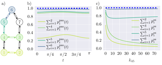
Figure 2: Inference of occupation probabilities of boundary states. a) Network with hidden states and hidden (black) transitions. Beginning with the light green transitions $(12)$ and $(21)$ in a), darker colored transitions are successively considered as observable. b) The sums of occupation probabilities of states within the boundary of each hidden network in the PSS are shown in the respective color. The time-dependent transition rates are given in Appendix A.1. c) As in b) but for constant driving, i.e., for a NESS as a function of $k_{45}$ with the other rates given in Appendix A.1.

Through equations (10) and (11) we show how to infer occupation probabilities of boundary states of the hidden network. Given the inferable quantities $p_{i}^{\text{pss}}(t_{0})$ or $p_{i}^{\text{ss}}$, we can calculate how much probability rests on states in the network beyond the so identified boundary states. As an example, Figures 2 b) and c) illustrate the probability to find the network shown in Figure 2 a) in its boundary states rather than in states within the interior of the hidden network. In both figures, different sets of observable transitions lead to different boundaries of the hidden network. Figure 2 b) displays sums of probabilities for these systems in a PSS, while Figure 2 c) gives an example for NESSs. Each sum of inferable occupation probabilities quantifies the probability of finding the system in the boundary of the hidden network. The closer this sum is to one, the less relevant the inaccessible states in the interior of the hidden network are for the dynamics.

4 Three estimators for entropy production in PSSs

In this section, we estimate irreversibility via the entropy production rate in a PSS. We have seen above how waiting-time distributions contain information on the hidden dynamics of a network. Thus, it seems sensible to expect that these quantities can be used as entropy estimator to infer irreversibility in both the observable and the hidden parts of the network.

For a trajectory $\Gamma$ of length $T$, reversing the driving protocol leads to transition rates $\tilde{k}_{ij}(t)=k_{ij}(T-t)$. The corresponding waiting-time distributions $\tilde{\psi}_{\tilde{J}\to\tilde{I}}(t|t_{0}+t)$ for reversed paths $\tilde{J}\to\tilde{I}$ are the time-reversed versions of $\psi_{I\to J}(t|t_{0})$. Once waiting-time distributions of the form $\tilde{\psi}_{\tilde{J}\to\tilde{I}}(t|t_{0}+t)$ have been determined, the fluctuation relation

$$\hat{\sigma}_{\psi}\equiv\lim_{T\to\infty}\frac{1}{T}\ln\frac{\mathcal{P}\left[\Gamma\right]}{\widetilde{\mathcal{P}}[\widetilde{\Gamma}]}$$ (12)

for a trajectory $\Gamma$ of length $T$ and its time-reverse $\widetilde{\Gamma}$ allows us to derive an estimator $\left\langle\hat{\sigma}_{\psi}\right\rangle_{\text{pss}}$ that fulfills

$$\left\langle\sigma\right\rangle_{\text{pss}}\geq\left\langle\hat{\sigma}_{\psi}\right\rangle_{\text{pss}}=\sum_{I,J}\int_{0}^{\infty}\int_{0}^{\mathcal{T}}\frac{n_{I}(t_{0})}{\mathcal{T}}\psi_{I\to J}(t|t_{0})\ln\frac{\psi_{I\to J}(t|t_{0})}{\tilde{\psi}_{\tilde{J}\to\tilde{I}}(t|t_{0}+t)}\differential{t_{0}}\differential{t}\geq 0.$$ (13)

Here, the index $\psi$ of the estimator highlights the type of waiting-time distribution that enters its expression in the above inequality. We prove this inequality in Appendix B as a generalization of the trajectory-based entropy estimator $\left\langle\hat{\sigma}\right\rangle$ introduced in [19] for NESSs.

For time-symmetric driving, estimating $\left\langle\sigma\right\rangle_{\text{pss}}$ with $\left\langle\hat{\sigma}_{\psi}\right\rangle_{\text{pss}}$ does not require to reverse the driving protocol in an experiment. In this case, $\tilde{\psi}_{\tilde{J}\to\tilde{I}}(t|t_{0}+t)$ results from $\psi_{I\to J}(t|t_{0})$ by exploiting the symmetry $k_{ij}(t_{*}+t_{0})=k_{ij}(t_{*}-t_{0})$ of the protocol for all transitions $(ij)$ after finding $t_{*}\in[0,\mathcal{T})$. In the next paragraphs, we discuss experimentally accessible entropy estimators that do not require waiting-time distributions of the time-reversed process regardless of symmetry properties of the driving.

We have performed extensive numerical computations of random, periodically driven Markov networks corresponding to different underlying graphs to compute

$$\left\langle\hat{\sigma}_{\Psi}\right\rangle_{\text{pss}}\equiv\sum_{I,J}\left\langle n_{I}\right\rangle_{\text{pss}}\int_{0}^{\infty}\Psi_{I\to J}(t)\ln\frac{\Psi_{I\to J}(t)}{\Psi_{\tilde{J}\to\tilde{I}}(t)}\differential{t},$$ (14)

where the index $\Psi$ indicates the type of waiting-time distribution used. Here, $\left\langle n_{I}\right\rangle_{\text{pss}}$ is the mean of $n_{I}(t_{0})$ in one period $t_{0}\in[0,\mathcal{T}]$ that results from measured data. For over $10^{5}$ randomly chosen systems from unicyclic graphs of three states, diamond-shaped graphs as displayed in Figure 1 a) and more complex underlying graphs, the inequalities

$$\left\langle\sigma\right\rangle_{\text{pss}}\geq\left\langle\hat{\sigma}_{\Psi}\right\rangle_{\text{pss}}\geq 0$$ (15)

hold true as shown in the scatter plot in Figure 3 a). Therefore, we conjecture inequality (15) to hold true for periodically driven Markov networks, so that $\left\langle\hat{\sigma}_{\Psi}\right\rangle_{\text{pss}}$ is a thermodynamically consistent estimator of $\left\langle\sigma\right\rangle_{\text{pss}}$.

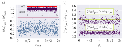
Figure 3: Ratios $\left\langle\sigma\right\rangle_{\text{pss}}/\left\langle\hat{\sigma}_{\Psi}\right\rangle_{\text{pss}}$ and $\left\langle\hat{\sigma}_{pk}\right\rangle_{\text{pss}}/\left\langle\hat{\sigma}_{\Psi}\right\rangle_{\text{pss}}$ involving entropy estimators in scatter plots. a) Quality factor $\left\langle\hat{\sigma}_{\Psi}\right\rangle_{\text{pss}}/\left\langle\sigma\right\rangle_{\text{pss}}$ for two data sets of networks with diamond-shaped graph as shown in Figure 1 a). b) Comparison between $\left\langle\hat{\sigma}_{pk}\right\rangle_{\text{pss}}$ and $\left\langle\hat{\sigma}_{\Psi}\right\rangle_{\text{pss}}$ for unicyclic three-state systems. The ratios in both scatter plots are plotted against the random angle $\varphi_{0}$ that is part of the free energy parametrization as detailed in Appendix A.2.

Furthermore, transition rates and occupation probabilities that are inferred as described in Section 3 allow us to prove another lower bound on the entropy production rate of a Markov network in a PSS which complements the previous two. The estimator

$$\left\langle\hat{\sigma}_{pk}\right\rangle_{\text{pss}}\equiv\int_{0}^{\mathcal{T}}\sum_{ij\in\mathcal{V}}\frac{p^{\text{pss}}_{i}(t)k_{ij}(t)}{\mathcal{T}}\ln\frac{p^{\text{pss}}_{i}(t)k_{ij}(t)}{p^{\text{pss}}_{j}(t)k_{ji}(t)}\differential{t}$$ (16)

adds up the contributions to entropy production along transitions of the set $\mathcal{V}$ containing all transitions that are either observable or within the boundary of the hidden network. As $\left\langle\hat{\sigma}_{pk}\right\rangle_{\text{pss}}$ solely depends on inferable probabilities and rates, its index is $pk$. Since each of the terms in Equation (16) is non-negative for all $t$ and part of $\left\langle\sigma\right\rangle_{\text{pss}}$ as given in Equation (3), $\left\langle\hat{\sigma}_{pk}\right\rangle_{\text{pss}}$ constitutes a lower bound on the total entropy production rate of the system. This bound may often be less tight than the conjectured bound (14) for periodically driven Markov networks though this ordering does not hold in general as shown in Figure 3 b).

In the special case of a NESS, the last bound (16) acquires the familiar form

$$\left\langle\hat{\sigma}_{pk}\right\rangle_{\text{pss}}\overset{\text{NESS}}{=}\sum_{ij\in\mathcal{V}}p^{\text{ss}}_{i}k_{ij}\ln\frac{p^{\text{ss}}_{i}k_{ij}}{p^{\text{ss}}_{j}k_{ji}}.$$ (17)

The crucial part is that here the entropy estimator $\left\langle\hat{\sigma}_{pk}\right\rangle_{\text{pss}}$ is based on occupation probabilities and transition rates inferred from distributions of waiting times between observable transitions as described in Section 3. Although the term (17) shows superficial similarities to the main result of reference [35] interpreted as an entropy estimator, our estimator $\left\langle\hat{\sigma}_{pk}\right\rangle_{\text{pss}}$ differs in two ways. First, $\left\langle\hat{\sigma}_{pk}\right\rangle_{\text{pss}}$ can be used for partially accessible Markov networks in a PSS, which include systems in a NESS as special cases. Second, the sum in Equations (16) and (17) includes contributions of both observable transitions and transitions within the boundary of the hidden network. These additional contributions allow for a more accurate estimate of the entropy production rate.

5 Concluding perspective

In this paper, we have introduced inference methods based on distributions of waiting times between consecutive observed transitions in partially accessible, periodically driven Markov networks. Successive use of these methods yields information about the kinetics of such a Markov network as well as its underlying topology, including hidden parts, as summarized in Figure 4.

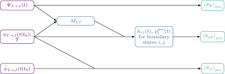
Figure 4: Summary of the inference scheme. Starting from waiting-time distributions and the known period $\mathcal{T}$ of the driving, the number of hidden transitions $M_{IJ}$ along the shortest path between two observable transitions $I$ and $J$, the occupation probabilities of boundary states $p_{i}^{\text{pss}}(t)$ as well as the rates $k_{ij}(t)$ of transitions between boundary states are inferable. These quantities enter the three lower bounds on entropy production.

We have first shown how to infer the number of hidden transitions along the shortest path between two observable transitions. We have then derived methods to infer transition rates between boundary states of the hidden network. Occupation probabilities of these boundary states then follow by discerning when the observable transitions happen within one period. Consequently, we find the total probability resting on the hidden states in the interior of the hidden network.

In addition, we have presented three entropy estimators enabling us to estimate irreversibility of a driven Markov network based on observed transitions during a partially accessible dynamics. The first and third one are proven to be lower bounds of the mean entropy production rate, whereas we conjecture the second estimator to have this property too. Its proof remains as open theoretical challenge. The second and third estimator have the advantage of not requiring control of the driving since its time reversal is not needed. Furthermore, we emphasize that even for the simpler NESS most of these results are original as well.

Finally, it will be interesting to explore whether and how such an approach can be adapted to continuous systems described by a Langevin dynamics. We also hope that our non-invasive method yielding time-dependent transition rates and occupation probabilities will be applied to experimental data of periodically driven small systems.

Appendix A Parameters used for numerical data

A.1 Parameters for data shown in Figure 2

For the network shown in Figure 2 a), the PSS is generated with transition rates

$$k_{ij}(t)=\kappa_{ij}e^{\left(F_{i}(t)-F_{j}(t)+f_{ij}\right)/2} k_{ji}(t)=\kappa_{ij}e^{-\left(F_{i}(t)-F_{j}(t)+f_{ij}\right)/2}.$$ and (18)

Therein, we set all $\kappa_{ij}=1$ as well as $f_{12}=f_{23}=f_{34}=f_{41}=2$ and $f_{45}=f_{56}=f_{67}=f_{73}=20/3$. Furthermore, we choose the free energies

$$F_{1}(t) =1.0+0.3\cos{2t}, F_{2}(t) =1.9+0.5\sin{2t},$$

$$F_{3}(t) =1.4+0.4\sin{2t}, F_{4}(t) =1.0+0.7\sin{2t},$$

$$F_{5}(t) =3.1+0.1\sin{2t}, F_{6}(t) =1.8+0.3\sin{2t},$$

$$F_{7}(t) =2.5$$ (19)

and solve the master equation (2) of the network for the occupation probabilities $p_{i}^{\text{pss}}(t)$.

The NESSs for this network as shown in Figure 2 c) are generated with the non-zero transition rates $k_{12}=1.7,\ k_{14}=0.4,\ k_{21}=0.6,\ k_{23}=3.5,\ k_{32}=0.3,\ k_{34}=3.3,\ k_{37}=0.02,\ k_{41}=5.7,\ k_{43}=0.3,\ k_{54}=0.1,\ k_{56}=0.7,\ k_{65}=0.2,\ k_{67}=0.8,\ k_{73}=4.6,\ k_{76}=0.05$ and $k_{45}\in[0.2,75]$.

A.2 Parameters for data shown in Figure 3

For Figure 3 a), we have used diamond-shaped networks as shown in Figure 1 a) but with observable transitions $1\leftrightarrow 2$ and $1\leftrightarrow 4$. For Figure 3 b), we have used unicyclic three-state systems with observable transitions $1\leftrightarrow 2$. All transition rates are parameterized as in Equation (18) with $\kappa_{ij}=1$ unless otherwise specified.

All diamond-shaped systems are characterized by $f_{12}=f_{14}=f_{23}=f_{31}=f_{43}=2$. The free energies of the states in each simulated diamond network are given by

$$F_{1}(t) =F_{c1}+F_{a1}\sin{\omega t}$$ (20)

$$F_{2}(t) =F_{c2}+F_{a2}\sin(n_{\omega,2}\omega t+\varphi_{0,2})$$ (21)

$$F_{3}(t) =F_{c3}+F_{a3}\sin(n_{\omega,3}\omega t+\varphi_{0,3})$$ (22)

$$F_{4}(t) =F_{c4}+F_{a4}\sin(n_{\omega,4}\omega t+\varphi_{0,4}),$$ (23)

where constant energies $F_{ci}$, energy amplitudes $F_{ai}$ and the angles $\varphi_{0,i}$ are randomly picked from normal distributions with mean and variance as given in Table 1.

Table 1: Mean and variance of the normal distribution corresponding to the two parameter sets, indigo and blue, defining all systems with diamond-shaped graph used for the scatter plot in Figure 3 a).

	$F_{c1}$	$F_{c2}$	$F_{c3}$	$F_{c4}$	$F_{a1}$	$F_{a2}$	$F_{a3}$	$F_{a4}$	$\varphi_{0,2}$	$\varphi_{0,3}$	$\varphi_{0,4}$
mean	1.58	3.05	1.84	1.64	$-0.01$	$-0.04$	0.05	0.11	4.39	4.79	$-17.93$
variance	0.5				0.005				5
mean	1.25	2.75	1.24	1.34	$-0.01$	$-0.27$	$-0.02$	$-0.01$	2.62	3.51	$-13.29$
variance	0.5				2.5				5

For $j\in\{1,\dots 4\}$, normally distributed $r_{j}\sim\mathcal{N}(0,1)$ define

$$\omega =25.27+5\absolutevalue{r_{1}} \omega=24.67+5\absolutevalue{r_{1}}$$ or (24)

for the data set plotted in indigo and in blue, respectively, and for both data sets

$$n_{\omega,i}=\lfloor 1+1.5\absolutevalue{r_{i}}\rfloor.$$ (25)

With the exception $k_{13}=1$ and $k_{31}=\exp\left[-F_{1}(t)+F_{3}(t)+f_{31}\right]$, the transition rates of the three-state networks used for Figure 3 b) are given by Equation (18) with $\kappa_{ij}=1$ and $f_{12}=f_{23}=f_{31}=2$. Moreover, the parameters in the free energies

$$F_{1}(t) =F_{c1}+F_{a1}\sin{\omega t}$$ (26)

$$F_{2}(t) =F_{c2}+F_{a2}\sin(n_{\omega}\omega t+\varphi_{0})$$ (27)

$$F_{3}(t) =F_{c3}$$ (28)

are normally distributed with mean and variance as listed in Table 2.

Table 2: Mean and variance of the normal distribution corresponding to the parameters defining the systems used for the scatter plot in Figure 3 b).

	$F_{c1}$	$F_{c2}$	$F_{c3}$	$F_{a1}$	$F_{a2}$	$\varphi_{0}$
mean	1.493	0.728	1.568	0.835	$-0.349$, $-3.49$	23.2
variance	0.5					5

The normally distributed $r_{j}\sim\mathcal{N}(0,1)$ for $j=1,2$ define

$$\omega =3.815+5\absolutevalue{r_{1}} n_{\omega}=\lfloor 1+1.5\absolutevalue{r_{2}}\rfloor.$$ and (29)

In all cases, we have computed the entropy production rate $\left\langle\sigma\right\rangle_{\text{pss}}$ through equation (3). For Figure 3 b), we have also calculated $\left\langle\hat{\sigma}_{pk}\right\rangle_{\text{pss}}$ via Equation (16), to which only transitions $(12)$ and $(21)$ contribute. Integrating initial value problems of the absorbing network, where observed transitions are redirected into auxiliary states [19, 36], yields waiting-time distributions $\psi_{I\to J}(t|t_{0})$. Using the previously obtained probabilities and transition rates, the estimator $\left\langle\hat{\sigma}_{\Psi}\right\rangle_{\text{pss}}$ can be determined after integrating out the phase-like time on which all waiting-time distributions depend.

Appendix B Proof for the entropy estimator (13)

The observed pairs of directed transitions yield coarse-grained trajectories $\Gamma(t)$

$$(I_{0},t_{0_{0}}=0)\overset{\Delta t_{1}}{\longrightarrow}(I_{1},t_{0_{1}}=t_{0}+\Delta t_{1}\mod\mathcal{T})\overset{\Delta t_{2}}{\longrightarrow}(I_{2},t_{0_{2}})\dots\overset{\Delta t_{N}}{\longrightarrow}(I_{N},t_{0_{N}})$$ (30)

of length $T$ in time, where we choose the starting time of a period such that we observe the first transition at $t_{0_{0}}=0$. A trajectory consists of tuples of observed transition $I_{i}$ and the phase-like time $t_{0_{i}}$ of its observation as well as of waiting times $\Delta t_{i}$ inbetween. During $\Delta t_{i}$, an arbitrary number of hidden transitions can occur. Moreover, as we know $\mathcal{T}$, we know the state of the network directly after each instantaneous transition. Thus, the next observable transition is independent of the past, i.e., the system has the Markov property at observable transitions. Therefore, the path weight of coarse-grained trajectories $\Gamma(t)$ factors into

$$\mathcal{P}\left[\Gamma(t)\right]=\mathcal{P}(I_{0},0)\psi_{I_{0}\to I_{1}}(\Delta t_{1}|0)\psi_{I_{1}\to I_{2}}(\Delta t_{2}|t_{0_{1}})\dots\psi_{I_{N-1}\to I_{N}}(\Delta t_{N}|t_{0_{N-1}}).$$ (31)

This factoring introduces waiting-time distributions of the form

$$\psi_{I\to J}(\Delta t|t_{0})\equiv\mathcal{P}\left[\Gamma_{I\to J}(\Delta t,t_{0})\middle|I,t_{0}\right]=\sum_{\gamma_{I\to J}\in\Gamma_{I\to J}}\mathcal{P}\left[\gamma_{I\to J}(\Delta t,t_{0})\middle|I,t_{0}\right]$$ (32)

defined in Equation (4) in terms of conditional path weights of microscopic trajectories $\gamma_{I\to J}(\Delta t,t_{0})$ that start right after an observed transition $I$ and end with the next observed transition $J$.

The time-reversed process results from reversing the protocol, the trajectory and the time. For a trajectory $\Gamma(t)$ of length $T$ that starts at the phase-like time $t_{0}$, the time-reversed transition rates read $\tilde{k}_{ij}(t)=k_{ij}(T-t)$ while the time transforms as $\tilde{t}=T-t$. Similarly, all quantities obtained by time-reversal will be marked with a tilde. The path weight of the time-reversed trajectory $\widetilde{\Gamma}$ is, in analogy to Equation (31), given by

$$\widetilde{\mathcal{P}}\left[\widetilde{\Gamma}(t)\right] =\widetilde{\mathcal{P}}\left(\tilde{I}_{N+1},T\right)\tilde{\psi}_{\tilde{I}_{N}\to\tilde{I}_{N-1}}(\Delta t_{N}|t_{0_{N-1}}+\Delta t_{N})\dots\tilde{\psi}_{\tilde{I}_{1}\to\tilde{I}_{0}}(\Delta t_{1}|0+\Delta t_{1}).$$ (33)

Similar to reference [37], we estimate the entropy production rate $\left\langle\sigma\right\rangle_{\text{pss}}$ using the log-sum inequality (see, e.g., [38]) as

$$T\left\langle\sigma\right\rangle_{\text{pss}} =\sum_{\zeta}\mathcal{P}\left[\zeta(t)\right]\ln\left(\frac{\mathcal{P}\left[\zeta(t)\right]}{\widetilde{\mathcal{P}}\left[\tilde{\zeta}(t)\right]}\right)$$

$$=\sum_{\zeta,\Gamma}\mathcal{P}\left[\Gamma(t)\middle|\zeta(t)\right]\mathcal{P}\left[\zeta(t)\right]\ln\left(\frac{\mathcal{P}\left[\Gamma(t)\middle|\zeta(t)\right]\mathcal{P}\left[\zeta(t)\right]}{\widetilde{\mathcal{P}}\left[\widetilde{\Gamma}(t)\middle|\tilde{\zeta}(t)\right]\widetilde{\mathcal{P}}\left[\tilde{\zeta}(t)\right]}\right)$$

$$\geq\sum_{\zeta,\Gamma}\mathcal{P}\left[\Gamma(t)\middle|\zeta(t)\right]\mathcal{P}\left[\zeta(t)\right]\ln\left(\frac{\sum_{\zeta}\mathcal{P}\left[\Gamma(t)\middle|\zeta(t)\right]\mathcal{P}\left[\zeta(t)\right]}{\sum_{\tilde{\zeta}}\widetilde{\mathcal{P}}\left[\widetilde{\Gamma}(t)\middle|\tilde{\zeta}(t)\right]\widetilde{\mathcal{P}}\left[\tilde{\zeta}(t)\right]}\right)$$

$$\equiv T\left\langle\hat{\sigma}_{\psi}\right\rangle_{\text{pss}}.$$ (34)

Here, $\mathcal{P}\left[\Gamma(t)\middle|\zeta(t)\right]=1=\widetilde{\mathcal{P}}\left[\widetilde{\Gamma}(t)\middle|\tilde{\zeta}(t)\right]$ holds if $\Gamma(t)$ is the correct coarse-grained trajectory onto which $\zeta(t)$ is mapped under coarse-graining. Otherwise, these conditional path weights vanish.

Replacing the sums of conditional path weights in the logarithm of the second line of inequality (34) with waiting-time distributions as in Equations (31) and (33) yields

$$\ln\left(\frac{\mathcal{P}\left[\Gamma(t)\right]}{\widetilde{\mathcal{P}}\left[\widetilde{\Gamma}(t)\right]}\right) =\underbrace{\ln\left(\frac{\mathcal{P}\left(I_{0},t_{0_{0}}\right)}{\widetilde{\mathcal{P}}\left(\tilde{I}_{N},T\right)}\right)}_{\equiv\delta(T,t_{0_{0}})}+\sum_{j=1}^{N}\ln\left(\frac{\psi_{I_{j-1}\to I_{j}}(\Delta t_{j}|t_{0_{j-1}})}{\tilde{\psi}_{\tilde{I}_{j}\to\tilde{I}_{j-1}}(\Delta t_{j}|t_{0_{j}}=t_{0_{j-1}}+\Delta t_{j})}\right).$$ (35)

The first term on the right hand side, $\delta(T,t_{0_{0}})$, is periodic when varying one of the fixed times $t_{0_{0}}$ and $T$. Hence $\absolutevalue{\delta(T,t_{0_{0}})}\leq c$ holds for a constant $c\in\mathbb{R}^{+}$.

To reformulate the sum on the right hand side of Equation (35), we define the conditional counter

$$\nu_{J|I}(t,t_{0})\equiv\frac{1}{T}\sum_{j=1}^{N}\delta(t-\Delta t_{j})\delta(t_{0}-t_{0_{j-1}})\delta_{I,I_{j-1}}\delta_{J,I_{j}}.$$ (36)

It sums all terms of trajectories that start with $I$ at $t_{0}$ and end with the succeeding observable transition $J$ after waiting time $t$. Substituting the conditional counter into Equation (35) leads to

$$\ln\left(\frac{\mathcal{P}\left[\Gamma(t)\right]}{\widetilde{\mathcal{P}}\left[\widetilde{\Gamma}(t)\right]}\right)=\delta(T,t_{0_{0}})+T\int_{0}^{\infty}\int_{0}^{\mathcal{T}}\sum_{I,J}\nu_{J|I}(t,t_{0})\ln\left(\frac{\psi_{I\to J}(t|t_{0})}{\tilde{\psi}_{\tilde{J}\to\tilde{I}}(t|t+t_{0})}\right)\differential{t_{0}}\differential{t}.$$ (37)

With $\lim_{T\to\infty}\absolutevalue{\delta(T,t_{0_{0}})}/T=0$, the calculation of the expectation value of Equation (37) reduces to determining the expectation value of the conditional counter. Following Ref. [19], we argue that

$$\nu_{J|I}(t,t_{0})\Delta t =\frac{\text{No. of transitions $(IJ)$ per $\mathcal{T}$ after $I$ at $t_{0}$ and waiting time $t\in[0,\Delta t]$}}{T}$$

$$=\frac{\text{No. of transitions $I$ per $\mathcal{T}$ at $t_{0}$}}{T}P(\text{$J$ after waiting time $t\in[0,\Delta t]$}|I,t_{0})$$ (38)

holds true. Together with $n_{I}(t_{0})/\mathcal{T}=\left\langle n_{I}\right\rangle_{\text{pss}}p^{\text{pss}}(t_{0}|I)$, this results in

$$\left\langle\nu_{J|I}(t,t_{0})\right\rangle =\sum_{\Gamma}\nu_{J|I}(t,t_{0})\mathcal{P}\left[\Gamma(t)\right]$$

$$=\frac{\left\langle\text{No. of transitions $I$ at $t_{0}$}\right\rangle/\mathcal{T}}{T}P(\text{$J$ after waiting time $t\in[0,\Delta t]$}|I,t_{0})$$

$$=\frac{n_{I}(t_{0})}{\mathcal{T}}\psi_{I\to J}(t|t_{0})=\left\langle n_{I}\right\rangle_{\text{pss}}p^{\text{pss}}(t_{0}|I)\psi_{I\to J}(t|t_{0}).$$ (39)

In total, the estimator $\left\langle\hat{\sigma}_{\psi}\right\rangle_{\text{pss}}$ of the mean entropy production rate is given by

$$\left\langle\hat{\sigma}_{\psi}\right\rangle_{\text{pss}} =\left\langle\lim_{T\to\infty}\frac{1}{T}\ln\left(\frac{\mathcal{P}\left[\Gamma(t)\right]}{\widetilde{\mathcal{P}}\left[\widetilde{\Gamma}(t)\right]}\right)\right\rangle$$

$$=\int_{0}^{\infty}\int_{0}^{\mathcal{T}}\sum_{I,J}\left\langle\nu_{J|I}(t,t_{0})\right\rangle\ln\left(\frac{\psi_{I\to J}(t|t_{0})}{\tilde{\psi}_{\tilde{J}\to\tilde{I}}(t|t+t_{0})}\right)\differential{t_{0}}\differential{t}$$

$$=\sum_{I,J}\int_{0}^{\infty}\int_{0}^{\mathcal{T}}\frac{n_{I}(t_{0})}{\mathcal{T}}\psi_{I\to J}(t|t_{0})\ln\left(\frac{\psi_{I\to J}(t|t_{0})}{\tilde{\psi}_{\tilde{J}\to\tilde{I}}(t|t+t_{0})}\right)\differential{t_{0}}\differential{t},$$ (40)

where the second equality follows from the vanishing $\delta(T,t_{0_{0}})/T$ in the limit $T\to\infty$. The estimator is non-negative as its definition (34) has the form of a Kullback-Leibler divergence. In the special case of a NESS, rewriting $\left\langle\hat{\sigma}_{\psi}\right\rangle_{\text{pss}}$ using Equation (39) reveals that this estimator reduces to $\left\langle\hat{\sigma}_{\Psi}\right\rangle_{\text{pss}}$, which we define in Equation (14), since then $p^{\text{pss}}(t_{0}|I)=1/\mathcal{T}$ and the waiting-time distributions do not depend on $t_{0}$.

References

- \bibcommenthead
- Seifert [2012] Seifert, U.: Stochastic thermodynamics, fluctuation theorems, and molecular machines. Rep. Prog. Phys. 75, 126001 (2012) https://doi.org/10.1088/0034-4885/75/12/126001
- Peliti and Pigolotti [2021] Peliti, L., Pigolotti, S.: Stochastic Thermodynamics. An Introduction. Princeton Univ. Press, Princeton and Oxford (2021)
- Shiraishi [2023] Shiraishi, N.: An Introduction to Stochastic Thermodynamics. Fundamental Theories of Physics. Springer, Singapore (2023). https://doi.org/10.1007/978-981-19-8186-9
- Rahav et al. [2008] Rahav, S., Horowitz, J., Jarzynski, C.: Directed flow in nonadiabatic stochastic pumps. Phys. Rev. Lett. 101, 140602 (2008) https://doi.org/10.1103/PhysRevLett.101.140602
- Chernyak and Sinitsyn [2008] Chernyak, V.Y., Sinitsyn, N.A.: Pumping restriction theorem for stochastic networks. Phys. Rev. Lett. 101, 160601 (2008) https://doi.org/10.1103/PhysRevLett.101.160601
- Raz et al. [2016] Raz, O., Subasi, Y., Jarzynski, C.: Mimicking nonequilibrium steady states with time-periodic driving. Phys. Rev. X 6, 021022 (2016) https://doi.org/%****␣papier.bbl␣Line␣125␣****10.1103/PhysRevX.6.021022
- Rotskoff [2017] Rotskoff, G.M.: Mapping current fluctuations of stochastic pumps to nonequilibrium steady states. Phys. Rev. E 95, 030101 (2017) https://doi.org/10.1103/PhysRevE.95.030101
- Stigler et al. [2011] Stigler, J., Ziegler, F., Gieseke, A., Gebhardt, J.C.M., Rief, M.: The complex folding network of single calmodulin molecules. Science 334(6055), 512–516 (2011) https://doi.org/10.1126/science.1207598
- Roldan and Parrondo [2010] Roldan, E., Parrondo, J.M.R.: Estimating dissipation from single stationary trajectories. Phys. Rev. Lett. 105, 150607 (2010) https://doi.org/10.1103/PhysRevLett.105.150607
- Muy et al. [2013] Muy, S., Kundu, A., Lacoste, D.: Non-invasive estimation of dissipation from non-equilibrium fluctuations in chemical reactions. The Journal of Chemical Physics 139(12), 124109 (2013) https://doi.org/10.1063/1.4821760
- Ge et al. [2012] Ge, H., Qian, M., Qian, H.: Stochastic theory of nonequilibrium steady states. part ii: Applications in chemical biophysics. Physics Reports 510(3), 87–118 (2012) https://doi.org/10.1016/j.physrep.2011.09.001 . Stochastic theory of nonequilibrium steady states (Part II): Applications in chemical biophysics
- Esposito [2012] Esposito, M.: Stochastic thermodynamics under coarse-graining. Phys. Rev. E 85, 041125 (2012) https://doi.org/10.1103/PhysRevE.85.041125
- Ariga et al. [2018] Ariga, T., Tomishige, M., Mizuno, D.: Nonequilibrium energetics of molecular motor kinesin. Phys. Rev. Lett. 121, 218101 (2018) https://doi.org/10.1103/PhysRevLett.121.218101
- Seifert [2019] Seifert, U.: From stochastic thermodynamics to thermodynamic inference. Ann. Rev. Cond. Mat. Phys. 10(1), 171–192 (2019) https://doi.org/10.1146/annurev-conmatphys-031218-013554
- Martínez et al. [2019] Martínez, I.A., Bisker, G., Horowitz, J.M., Parrondo, J.M.R.: Inferring broken detailed balance in the absence of observable currents. Nature Communications 10, 3542 (2019) https://doi.org/10.1038/s41467-019-11051-w
- Dechant and Sasa [2021] Dechant, A., Sasa, S.I.: Improving thermodynamic bounds using correlations. Phys. Rev. X 11, 041061 (2021) https://doi.org/10.1103/PhysRevX.11.041061
- Skinner and Dunkel [2021] Skinner, D.J., Dunkel, J.: Improved bounds on entropy production in living systems. Proc. Natl. Acad. Sci. U.S.A. 118(18) (2021) https://doi.org/10.1073/pnas.2024300118
- Harunari et al. [2022] Harunari, P.E., Dutta, A., Polettini, M., Roldan, E.: What to learn from a few visible transitions’ statistics? Phys. Rev. X 12, 041026 (2022) https://doi.org/10.1103/PhysRevX.12.041026
- van der Meer et al. [2022] van der Meer, J., Ertel, B., Seifert, U.: Thermodynamic inference in partially accessible markov networks: A unifying perspective from transition-based waiting time distributions. Phys. Rev. X 12, 031025 (2022) https://doi.org/10.1103/PhysRevX.12.031025
- van der Meer et al. [2023] van der Meer, J., Degünther, J., Seifert, U.: Time-resolved statistics of snippets as general framework for model-free entropy estimators. Phys. Rev. Lett. 130, 257101 (2023) https://doi.org/10.1103/PhysRevLett.130.257101
- Ohga et al. [2023] Ohga, N., Ito, S., Kolchinsky, A.: Thermodynamic bound on the asymmetry of cross-correlations. Phys. Rev. Lett. 131, 077101 (2023) https://doi.org/10.1103/PhysRevLett.131.077101
- Liang and Pigolotti [2023] Liang, S., Pigolotti, S.: Thermodynamic bounds on time-reversal asymmetry. Phys. Rev. E 108, 062101 (2023) https://doi.org/10.1103/PhysRevE.108.L062101
- Degünther et al. [2023] Degünther, J., van der Meer, J., Seifert, U.: Fluctuating entropy production on the coarse-grained level: Inference and localization of irreversibility (2023) arXiv:2309.07665 [cond-mat.stat-mech]. Phys. Rev. Res. in press
- Li and Kolomeisky [2013] Li, X., Kolomeisky, A.B.: Mechanisms and topology determination of complex chemical and biological network systems from first-passage theoretical approach. The Journal of Chemical Physics 139(14), 144106 (2013) https://doi.org/10.1063/1.4824392
- Van Vu and Saito [2023] Van Vu, T., Saito, K.: Topological speed limit. Phys. Rev. Lett. 130, 010402 (2023) https://doi.org/10.1103/PhysRevLett.130.010402
- Ito and Dechant [2020] Ito, S., Dechant, A.: Stochastic time evolution, information geometry, and the Cramér-Rao bound. Phys. Rev. X 10, 021056 (2020) https://doi.org/%****␣papier.bbl␣Line␣425␣****10.1103/PhysRevX.10.021056
- Shiraishi et al. [2018] Shiraishi, N., Funo, K., Saito, K.: Speed limit for classical stochastic processes. Phys. Rev. Lett. 121, 070601 (2018) https://doi.org/10.1103/PhysRevLett.121.070601
- Dechant et al. [2023] Dechant, A., Garnier-Brun, J., Sasa, S.-i.: Thermodynamic bounds on correlation times. Phys. Rev. Lett. 131, 167101 (2023) https://doi.org/10.1103/PhysRevLett.131.167101
- Barato and Seifert [2015] Barato, A.C., Seifert, U.: Thermodynamic uncertainty relation for biomolecular processes. Phys. Rev. Lett. 114, 158101 (2015) https://doi.org/10.1103/PhysRevLett.114.158101
- Gingrich et al. [2016] Gingrich, T.R., Horowitz, J.M., Perunov, N., England, J.L.: Dissipation bounds all steady-state current fluctuations. Phys. Rev. Lett. 116, 120601 (2016) https://doi.org/10.1103/PhysRevLett.116.120601
- Proesmans and van den Broeck [2017] Proesmans, K., van den Broeck, C.: Discrete-time thermodynamic uncertainty relation. EPL 119(2), 20001 (2017) https://doi.org/10.1209/0295-5075/119/20001
- Barato et al. [2018] Barato, A.C., Chetrite, R., Faggionato, A., Gabrielli, D.: Bounds on current fluctuations in periodically driven systems. New J. Phys. 20, 103023 (2018) https://doi.org/10.1088/1367-2630/aae512
- Koyuk and Seifert [2019] Koyuk, T., Seifert, U.: Operationally accessible bounds on fluctuations and entropy production in periodically driven systems. Phys. Rev. Lett. 122(23), 230601 (2019) https://doi.org/10.1103/PhysRevLett.122.230601
- Barato et al. [2019] Barato, A.C., Chetrite, R., Faggionato, A., Gabrielli, D.: A unifying picture of generalized thermodynamic uncertainty relations*. Journal of Statistical Mechanics: Theory and Experiment 2019(8), 084017 (2019) https://doi.org/10.1088/1742-5468/ab3457
- Shiraishi and Sagawa [2015] Shiraishi, N., Sagawa, T.: Fluctuation theorem for partially masked nonequilibrium dynamics. Phys. Rev. E 91, 012130 (2015) https://doi.org/10.1103/PhysRevE.91.012130
- Sekimoto [2022] Sekimoto, K.: Derivation of the first passage time distribution for markovian process on discrete network (2022) arXiv:2110.02216 [cond-mat.stat-mech]
- Gomez-Marin et al. [2008] Gomez-Marin, A., Parrondo, J.M.R., Van den Broeck, C.: Lower bounds on dissipation upon coarse-graining. Phys. Rev. E 78, 011107 (2008) https://doi.org/10.1103/PhysRevE.78.011107
- Cover and Thomas [2006] Cover, T.M., Thomas, J.A.: Elements of Information Theory. Telecommunications and signal processing. Wiley, Hoboken, NJ, and Canada (2006)