Exponential Error Reduction for Glueball Calculations Using a Two-Level Algorithm in Pure Gauge Theory
Abstract
This study explores the application of a two-level algorithm to enhance the signal-to-noise ratio of glueball calculations in four-dimensional pure gauge theory. Our findings demonstrate that the statistical errors exhibit an exponential reduction, enabling reliable extraction of effective masses at distances where current standard methods would demand exponentially more samples. However, at shorter distances, standard methods prove more efficient due to a saturation of the variance reduction using the multi-level method. We discuss the physical distance at which the multi-level sampling is expected to outperform the standard algorithm, supported by numerical evidence across different lattice spacings and glueball channels. Additionally, we construct a variational basis comprising 35 Wilson loops up to length 12 and 5 smearing sizes each, presenting results for the first state in the spectrum for the scalar, pseudoscalar, and tensor channels.
I Introduction
One consequence of confinement of quarks and gluons by the strong force in quantum chromodynamics (QCD) is the possible existence of glueballs [1, 2], states predominantly made of gluons. These hypothetical composites have been studied widely within a range of theoretical frameworks, such as the bag model [3, 4, 5, 6], flux-tube model [7, 8] and QCD sum rules [9, 10, 11, 12] and have been investigated from first principles since the development of lattice QCD methods [13, 14, 15, 16, 17]. Finding experimental evidence for glueballs remains a challenge [18] as the lightest candidates suggested by theoretical studies are rather massive, approaching twice the mass of a nucleon and have quantum numbers in common with some quark-model mesons. As a result, physical states at this energy scale are mixtures of conventional isoscalar mesons and glueballs and have large phase-space for decay to multiple light mesons [19, 20, 21, 22, 23]. Very little is known about the decay processes of the glueball in QCD, so reliable interpretation of resonances in collider experiments as glueballs is challenging. There have been a number of experimental observations of candidates [24], mostly identified as an over-population of resonances compared to quark model predictions, but their link to QCD remains unresolved. Recent experimental confirmation of pseudoscalar quantum numbers for the X(2370) [25] have given fresh incentive to these studies.
Lattice QCD calculations can provide a great deal of information to guide these searches from first principles. Ideally, the spectrum is computed on the lattice, including the dynamics of the quark and gluon fields [26, 27, 28, 29, 30, 31, 32] which causes both mixing of quark-model mesons with the glueballs and their strong decays. Then, widths of the resulting resonances can be studied following ideas introduced by Lüscher [33] which relate the energy spectrum in a finite volume to certain scattering phase shifts. Developing this framework beyond two-body elastic scattering is a very active research topic [34], but the input which lattice calculations must provide remains the accurate determination of a complete low-energy spectrum of QCD in a finite volume. This can only be computed in practice by determining two-point correlation functions between a broad range of creation and annihilation operators resembling glueballs, quark-model isoscalar mesons, two-pion states, and so on.
One difficulty with these calculations arises from use of importance-sampling Monte Carlo estimates. The spectrum is extracted from the Euclidean-time dependence of correlation functions, which fall exponentially with a rate governed by the energies of the states under investigation. In glueball calculations, the relevant scale is typically beyond 1.5 GeV. The Monte Carlo estimators have high statistical variance, roughly independent of the Euclidean time separation. As a result, the signal-to-noise ratio falls rapidly [35, 36] and very large statistical ensembles, typically with samples, are needed for high precision.
This study tests and models the behavior of improved Monte Carlo methods offering better signal-to-noise performance. Our investigation is restricted to the pure Yang-Mills theory; there is active research [37, 38, 39, 40, 41] into extensions of these techniques to QCD, including the dynamics of the quark fields outside the scope of this paper. Calculations with fermions present significant technical challenges as the resulting path integrals cannot be computed directly by Monte Carlo. Locality of the Yang-Mills action along with bosonic statistics of gluons allows factorization of the observables of the lattice field theory into sub-volume integrals, which can be sampled independently by drawing random field variables from the appropriate conditional distributions and constructing full observables with smaller variance from products of these independent samples. The first use of this factorization was the multi-hit algorithm [42], introduced in computations of the string tension. The algorithm was subsequently extended to multi-level methods [43], achieving exponential error reduction for certain observables. Later work [44, 45, 46, 47] investigated these schemes for glueball calculations where the temporal extent of the lattice is divided into nested subdomains and expectation values estimated by hierarchical Markov chain Monte Carlo calculations inside these layers.
The paper extends earlier work [48] testing these schemes in detail and is organized as follows. Section 2 reviews the multi-level sampling algorithm, focussing on determinations of glueball correlation functions. Section 3 presents the findings of our calculation, including detailed analysis of the performance of the method when using a large basis of operators suitable for spectrum calculations based on solving a generalized eigenvalue problem (GEVP) [49, 50, 51]. These techniques are the key to reliable studies when mixing with quarkonia or decays into multiple hadrons are investigated. Comparisons with state-of-the-art calculations are made, and statistical precision is studied in detail. Our conclusions are presented in Section 4.
II The multi-level sampling algorithm
Energy eigenstates can be investigated using two-point correlation functions of quantum fields on an Euclidean lattice. Their efficient determination in Monte Carlo calculation using a multi-level algorithm proceeds as follows.
II.1 Algorithmic details
The correlation function of two operators and is defined as
| (1) | ||||
where is the partition function, and is the Euclidean action. This integral can be estimated numerically with Monte Carlo techniques, by generating an ensemble of gauge configurations , drawn from a sample distribution with probability . We then estimate the correlation by computing
| (2) |
with the associated standard error
| (3) |
which depends on the decorrelated sample size and variance
| (4) |
Multi-level simulations, [42, 43, 44] were introduced after observing the path integral of the correlation function in a pure gauge theory factorizes into subdomains
| (5) | ||||
where we are using, in addition to the established expectation , the sub-average as defined in [43]
| (6) |
with
| (7) |
Here, we denote as gauge fields on fixed boundaries, while and are gauge fields whose dynamics are determined by the conditional actions and . The superscripts of and refer to the two different regions.
This decomposition splits the lattice into two independent domains depending on the fixed boundary separating them. The path integrals on the subdomains can then be approximated by simulating only the subdomain with fixed boundary conditions. In practice, we initially generate a regular Monte Carlo chain of configurations, denoted as for . These are referred to as level-0 configurations. The fields restricted to are subsequently distributed according to the marginal probability density in the integration in Eq. (5).
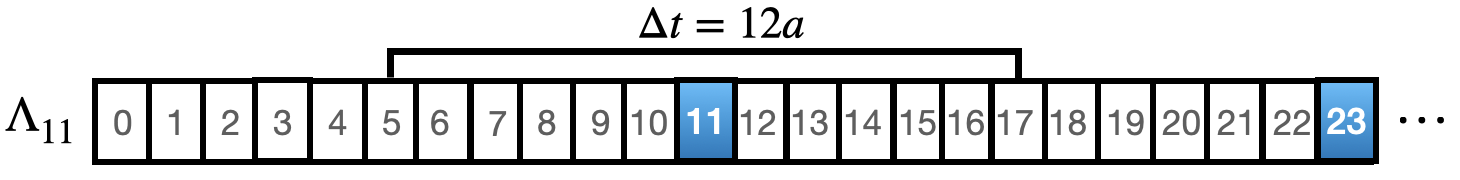
From each of these level-0 configurations, we generate a sub-chain of configurations updated in each sweep only on partial domains but left unchanged on the remaining temporal domains. These sub-chains are generated with fixed boundary conditions, drawn from the conditional probability density in the -integrals in Eq. (5). We refer to the updated domains as the dynamical regions, while the other time slices are the fixed regions, which separate two different dynamical ones. We use the notation to refer to the specific sub-lattice decomposition in dynamical and frozen regions of the sub-chains. In Fig. 1, there is one example of sub-lattice decompositions adopted in this work. The blue-shaded regions at , , (, ) are the fixed regions, consisting of only one time slice each, and the other time slices are the dynamical regions, where the fields are updated along the level-1 chain. The temporal gauge links connecting the fixed with the dynamical regions are updated. We label these level-1 configurations, using a second index to indicate the trajectory time along the sub-chains, while indicates the initial level-0 configuration. Thus we generate gauge configurations, labelled . Using the Wilson plaquette action, fixed regions comprised of a single time slice are sufficient to separate the dynamical regions such that gauge updates are independent, whereas for improved gauge actions which include larger Wilson loops such as the Lüscher-Weisz, the width of the frozen regions must be increased.
When the operators are in two different dynamical regions, the multi-level estimator reads
| (8) | |||
which corresponds to a combination of two independent level-1 averages followed by a level-0 average. We will confirm that this reduces noise sufficiently to make it equivalent to a standard measurement with samples up to boundary corrections. Then the error scales ideally like , as one can guess from the scaling of this estimator with and . Corrections to this ideal scaling are discussed in the following subsection. The factorization in Eq. (5) applies only when the operators are in two different regions.
When the operators are in the same region, and therefore when and belong to the same domain, the level-1 and level-0 measurements give a unique sample, and we have to employ the standard estimator
| (9) | |||
where at best the error scales like as in Eq. (3).
II.2 The noise-to-signal ratio
The spectral decomposition of the correlation functions, estimated with Monte Carlo algorithms using Eq. (2), exhibits an exponential decay of the signal over time as
| (10) | ||||
with , the energy of a state with the quantum numbers of the zero-momentum operator , and , the ground-state mass. Since in our investigation is a glueball operator, is the mass of the ground-state glueball.
The variance of a glueball correlation function computed with traditional algorithms is approximately constant [36, 35] as the source-sink separation varies. Thus, its noise-to-signal ratio increases exponentially as
| (11) |
and to keep the relative precision constant at all time separations, one must record measurements. However, if the correlation function is estimated with multi-level algorithms using Eq. (8), the noise-to-signal ratio becomes
| (12) |
where clearly, performing the additional sub-measurements keeps the relative error fixed much more efficiently. Indeed, performing more sub-measurements for each operator keeps the error fixed, as opposed to with the traditional algorithm. There is a clear exponential improvement.
However, the expression in Eq. (12) is correct up to fluctuations arising from the boundaries, i.e., the fixed regions, but will still be enough to keep the relative error constant, as we discuss below. In general, by taking into account fluctuations from the fixed boundaries, one can derive the expression for the variance of the multi-level correlation function [52], which reads
| (13) | ||||
with of similar order of magnitude. In this formula, and denote the distance of the operators at or respectively to the nearest boundaries at .
Eq. (13) contains important information on the dependence of multi-level algorithm performance on the parameter choice. The time-independent term of the multi-level error scales with , up to exponential fluctuations induced by the fixed boundaries. The multi-level error decreases with the number of sub-measurements until the last term in Eq. (13), which is independent of , becomes relevant. Note the formula in Eq. (13) accounts only for fluctuations from one nearest boundary for each operator, while in general, one has to consider all the boundary fluctuations.
We must emphasize an important caveat: Numerically, we find that the mass in the exponent of the boundary fluctuations corresponds to twice the mass of a glueball state, , in that particular glueball channel . In all glueball channels, we expect states with vacuum quantum numbers to contribute at long distances and to be suppressed at short distances due to small overlap. Unfortunately, we do not have sufficient data to show this.
II.3 Saturation of the variance reduction
The multi-level error reduction is explicitly dependent on the level-1 sub-measurements and the distance of the operators from the nearest boundaries. In particular, there is a critical number of sub-measurements , above which the multi-level error does not reduce further with . This saturation point is reached when the first two terms in Eq. (13) become the same order of magnitude as the last.
As a result, for operators symmetrically distant from the boundaries, i.e. , with and , the multi-level error decreases exponentially like and consequently the relative error stays constant with increasing . As noted in section II.2, we see here again the origin of the noise reduction: For the standard Monte Carlo method, we need to rescale the number of measurements with while now we need only more measurements in a multi-level simulation to achieve a constant relative error.
However, at short distance, this represents a limitation compared to the traditional error scaling. While the multi-level error is independent of for , the traditional scaling decreases as , modulo exponential fluctuations from the boundaries. Therefore, at short distance, it is better to measure the correlations between operators located in the same dynamical regions, whose error scales like the traditional scaling. There is an intermediate distance where the saturated multi-level starts to outperform the standard scaling. This occurs when
| (14) |
is satisfied. Our simulations confirm this behavior, as shown in the next section. For instance, on the ensemble gb62, it is clear from Figs. 3-4 the transition point for the channel with and is between .
The variance of the correlation function is clearly not the same for each , even at fixed . To take advantage of all the measurements for a given distance , we consider the weighted average
| (15) |
where we choose the weights . This weighted average selects the best correlation from either the standard correlation of operators in the same domain for short distances or multi-level correlations of operators separated equally from a fixed boundary in different domains for long distances. There is more discussion on optimum weighting for multi-level algorithms in [53].
Due to the weighted average, there is a transition between different error scalings: At sufficiently long distance , which depends on the glueball channel, c.f. Eq. (14), from Eq. (13) we expect the variance-to-signal ratio of the weighted average in Eq. (15) for a specific glueball channel to be
| (16) | ||||
where the term increasing exponentially with is divided by rather than , thus rendering a substantial improvement at large distance. At short distance, the noise-to-signal ratio of the weighted average is expected to scale like
| (17) |
where , c.f. Eq. (3). Thus, the weighted average exhibits two different scalings at short and long distances, and the transition between the two behaviors occurs when Eq. (14) is fulfilled.
III Simulations
The performance of the multi-level method was examined in several numerical computations of a lattice discretisation of SU(3) Yang-Mills theory as described in this section.
III.1 Details
We simulate the Wilson pure gauge action
| (18) |
with periodic boundary conditions, and we investigate , , with a physical volume kept roughly constant to using a modified version of OpenQCD [54, 55]. See Tab. 1 for an overview of the ensembles analyzed in this work.
| Name | Level-1 decomposition | ||||
|---|---|---|---|---|---|
| gb62 | 48 | 24 | 6.2 | ||
| gb608 | 40 | 20 | 6.08 | ||
| gb58 | 24 | 12 | 5.8 |
For each , we generate gauge configurations with the traditional HMC algorithm, i.e., the gauge configurations are updated on the entire volume. We choose well spaced configurations such that the autocorrelations are negligible. For each of these level-0 configurations, a new, independent Monte Carlo chain is generated using HMC, as discussed in section II.1. In particular, on the ensemble gb62 at , with , , the level-1 gauge configurations are kept fixed on time slices , while updated everywhere else. This way, there are four regions where the gauge fields are updated independently. This decomposition is labelled since the dynamic regions comprise lattice sites, corresponding to each, as seen in Fig. 1. Since we are interested in the glueball spectrum, the observable is a glueball operator, which in pure gauge theory can be constructed from Wilson loops. Appendix A gives more detail on constructing glueball operators projected onto a specific lattice irreducible representation of the group of rotations of the cube with parity and charge conjugation . This work investigates , and . For each operator we estimate the correlation function using Eq. (8) when the operators are in two different regions, while when the operators are in the same region, we estimate the correlation function using Eq. (9). When the two operators are in different dynamic regions, the error should scale according to Eq. (13). However, if the operators are in the same region, the error is almost constant over time and should scale like , see Eq. (3).
III.2 Analysis of the statistical precision
Fig. 2 shows the standard error of the correlation function for at (top), and (bottom) for different values of . The source operator is fixed at while the sink operator at is moved to determine the dependence of the error on the distance of the sink from the boundaries.
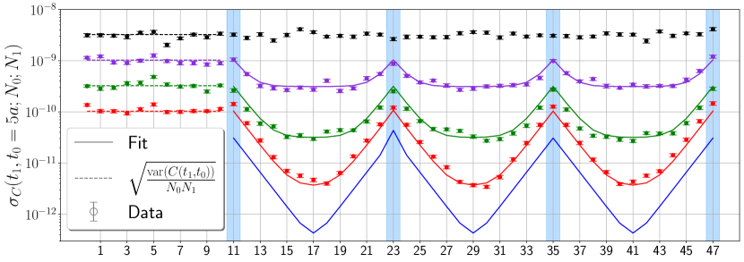
The correlation function is computed on the ensemble gb62 using the level-1 decomposition , see Fig. 1. When the two operators are measured in different regions, the statistical uncertainty follows a behavior as the operator moves between adjacent boundaries. As the large limit is approached, the error decreases exponentially according to when . In contrast, when the operators are in the same dynamical region , statistical fluctuations are independent of separation, so the uncertainty falls only in inverse proportion to . Using a global fit of the data to Eq. (13), we find . This model behavior is compared to our data on the figure along with the limiting behavior when . In this limit, the third term in the expression, independent of , persists, which suggests sub-sampling more than measurements does not improve precision any further.
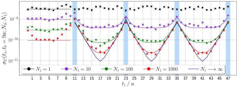
The four panels of Fig. 3 show the dependence of the error on the operator location relative to the boundaries for different values of , for and . As before, for certain values of , the two operators are in the same sampling region, so the error is proportional to . In contrast, for values of where the operators are in different regions, the error behaves according to Eq. (13). The x-axis is chosen so operators symmetrically distant from the boundaries are horizontally aligned, emphasizing the error reduction at different values of . At short distance, the multi-level error saturates at . For the channel on ensemble gb62, this corresponds to and for , respectively. Note the largest error reduction occurs when the two operators are at equal distances from the boundaries (). This is seen in Fig. 3, where the multi-level error saturates at the red dashed line for . As a result, it is more efficient to determine the correlation function at short distances from operator pairs in the same dynamical region rather than adopting the multi-level since the standard error reduction, is larger than the multi-level reduction after saturation. Beyond , Fig. 3 shows that the multi-level scheme is more efficient than standard Monte Carlo.
III.3 Universal scaling toward the continuum limit
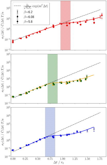
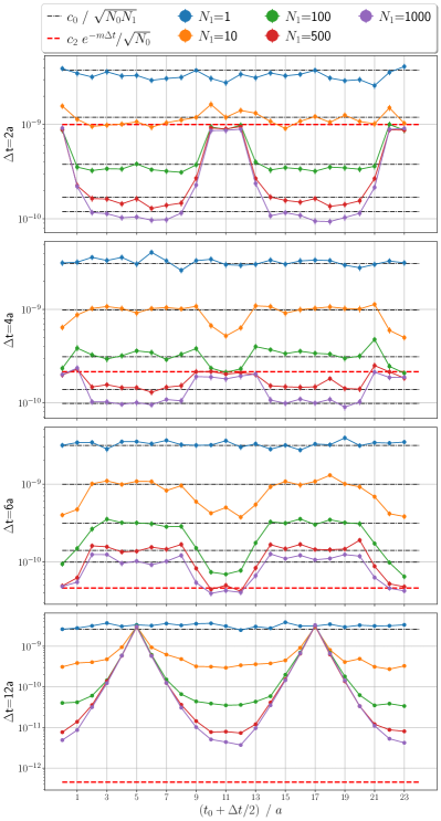
We investigate the scaling of the multi-level algorithm toward the continuum limit ( and ) for the glueball channels , , , and . For each correlator computed at different and , we consider the weighted average in Eq. (15). Fig. 4 shows the noise-to-signal ratio of the weighted average glueball correlation functions in units of for a single glueball operator in all four channels. The data shows that at small distance () the noise-to-signal ratio increases exponentially like , which is the standard scaling with traditional algorithms. The reason is at short distance, the multi-level error reduction is not large, as observed in Fig. 3, so operators located in the same region contribute more to the weighted average, because their statistical errors are smaller. It is important to mention that if one considers only operators located in two different dynamic regions, the resulting relative errors of the weighted average would be constant from to or depending on the channel. This is because the multi-level error saturates at large at a value of , which is also how the signal drops over time. At intermediate time separations (), there is a change of scaling where the noise-to-signal ratio is almost constant. This region is highlighted by the shaded blue band in Fig. 4. The physical distance where the transition occurs is universal for each channel, as expected from Eq. (14) because does not depend on . The dependence on the mass can be observed between the channel and the other channels, the former contains the lightest state in the spectrum, thus requiring slightly larger time separations for the change of scaling. After this transition, the noise-to-signal ratio follows the multi-level scaling, i.e. the square root of Eq. (16), which is observed until the error of the error becomes too large. Thus, to keep the relative error constant over time at large separations, one has to set .
III.4 Spectrum results
To determine the glueball spectrum, we construct a basis consisting of Wilson loops with different shapes, as discussed in Appendix A, some of which can be projected onto the channels of interest , , , and as shown in [13, 57]. Each of these Wilson loops is built from links smeared with different APE smearing levels [58] to construct an efficient variational basis made of up to operators.
For each operator in this basis, we estimate the matrix of correlation functions
| (19) |
with a total of sub-measurements and denotes the number of distinct operators formed from combinations of Wilson loops projected onto irrep . We estimate the weighted average as discussed in the previous section, see Eq. (15). We then solve for the GEVP
| (20) | ||||
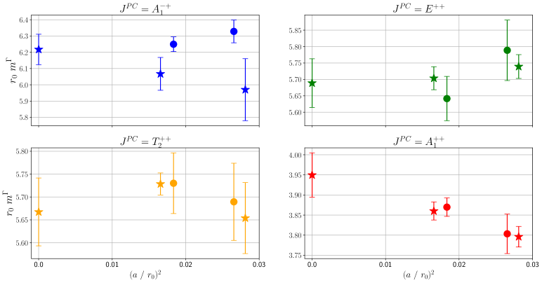
where and are the matrices of generalized eigenvalues and eigenvectors, respectively. The GEVP effective masses of ground state and further excitations can be extracted from the eigenvalues as for the channels [59, 60]. Some operators with different shapes might be degenerate at large enough smearing radii, as observed in Fig. 8 of [61], and thus some careful choice must be made for the optimal variational basis. Thus, we do not employ the full operator basis for each channel and, in practice, use operators for each glueball channel. We adopt the two-level algorithm on configurations with up to sub-measurements to compute these correlation functions and solve the GEVP. In Fig. 5, we present results at for the ground state of the different channels. The small irregularity at in the channel is a statistical fluctuation and is due to the loss of translational invariance of the error after combining multi-level with standard measurements. In particular, if the statistical error is slightly underestimated, it will enhance some correlators in the weighted average, as the weights are the inverse of the variance, see Eq. (15). A comparison with state-of-the-art results of [17] at similar values but slightly different volumes shows that the multi-level results have smaller errors at large source-sink separations due to better scaling, as shown in Fig. 4. In particular, in Fig. 6, we show a comparison between our multi-level results at , and the state-of-the-art results in [17] at , . The results agree within the errors, and the statistical uncertainty is also very similar.
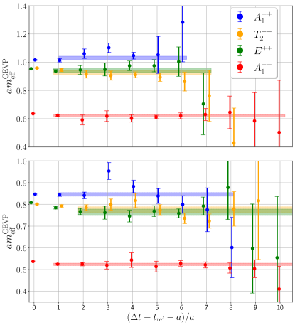
The statistics used in the two calculations are roughly the same (), along with the computational cost of all the updates ( MDUs), and we also adopt a large variational basis. Although the multi-level improves the noise-to-signal at large distance, c.f. Fig. 4, the algorithm does not improve the final uncertainty of the glueball effective masses. Glueball masses are extracted from a fit that starts at short distance, where the multi-level does not work efficiently. This explains why the uncertainty for the final value of the glueball effective masses is roughly similar to [17], see Fig. 6. However, the multi-level signal is determined to much longer distances where the ground state dominates, which gives more confidence in the reliability of the plateau estimated at short distance. The multi-level algorithm will be necessary for investigations of glueball mixing with quark-anti-quark mesons when dynamical fermions are included as the signal drops quickly and it is challenging to understand the gluonic content of the mixed states [62].
IV Conclusions
We have investigated the efficiency of a two-level algorithm for determining the glueball mass spectrum in various channels toward the continuum limit. It was not a priori clear that the method would be efficient. As we demonstrated, the standard estimator outperforms the two-level measurements at short distances. This is primarily due to the breaking of the translational invariance by the fixed boundaries and the effect of the fixed fields on them, which limit the exploration of field space in their vicinity. With the standard method, the noise-to-signal ratio deteriorates exponentially, and the signal could be lost before the two-level estimator becomes efficient. This is complicated further because state-of-the-art analyses combine correlation functions at various source-sink separations using a sizeable variational basis with a GEVP to extract effective masses. We have demonstrated that in this setting the two-level method works. The deterioration is stopped, and the noise-to-signal ratio stays constant for a certain time interval.
The results agree very well with state-of-the-art analyses that adopt the traditional Monte Carlo. The overall statistical uncertainty is not improved; however, the GEVP masses are extracted from fits starting at short time separation, where the two-level is ineffective. Still, with the same cost as traditional Monte Carlo, the two-level algorithm can render correlation functions at long distance with an exponentially reduced error, giving more confidence in the plateau estimate.
Depending on the channel, the two-level method is more efficient for source-sink separations above fm to fm, and we can extend the plateau region by roughly fm using sub-measurements. We can reliably model the performance of the algorithm depending on the source and sink position as well as the resulting weighted averages. This allows us to understand the transition in the dominance in the average from the standard to the two-level measurements with increasing time.
The two-level Monte Carlo is an expensive method. To offset the reduced averaging in time due to the fixed regions, the number of sub-measurements needs to be large, where the full power is only reached at significant source-sink separations. To ensure a reliable error analysis, boundary fields must be sampled with at least measurements. This requirement translates to a cost equivalent to taking measurements on gauge field configurations for .
Our study has been performed in pure gauge theory, where an operator basis can be found that allows plateau fits from very short time separations. In the presence of fermions, this is no longer possible. The large separations that can be reached with the two-level algorithm will become essential, for instance, in studies of glueball-charmonium mixing. Here standard algorithms cannot reach trustworthy plateau regions such that reliable computations need improved methods like the one investigated here.
Acknowledgements.
The work is supported by the German Research Foundation (DFG) research unit FOR5269 ”Future methods for studying confined gluons in QCD.” The authors thank all the members of the research unit for useful discussions. L. B. is grateful to J. Frison and A. Risch for discussions. S. M. received funding from the European Union’s Horizon 2020 research and innovation program under the Marie Skłodowska-Curie grant agreement №813942. This work was supported by the STRONG-2020 project, funded by the European Community Horizon 2020 research and innovation programme under grant agreement 824093. The authors gratefully acknowledge the scientific support and HPC resources provided by the Erlangen National High Performance Computing Center (NHR@FAU) of the Friedrich-Alexander-Universität Erlangen-Nürnberg (FAU) under the NHR project k103bf.Appendix A Construction of the glueball operators
The starting point to build the glueball operators used in this work is a given loop shape, e.g. the 22 different ones presented in [13] of lengths 4, 6 and 8. A 3D Wilson loop of fixed shape starting at spatial point and Euclidean time is denoted as , where the index labels the shape. Elements of the cubic group can act on such a Wilson loop when it is represented as a tuple of unitary displacements equivalent under cyclic permutations thanks to the projection to zero spatial momentum [13]. The loop obtained after acting with group element , , on is denoted as . Considering only the index and not any degeneracies between loops, these 24 loops form a basis which generates the regular (or permutation) representation of the cubic group, and therefore there exist linear combinations of them which transform according to any of the five irreps of this group [57, 63]. A glueball operator with zero spatial momentum which transforms according to a given irrep can be written as
| (21) |
where denotes the copy of irrep which appears in the regular representation and are the projection coefficients coefficients for copy of irrep . These coefficients can be calculated via projection methods [57, 63]. In this work we consider only one copy per irrep so we omit the index from now on. Parity is fixed by considering the sum or difference of each loop with its parity twin, i.e. the loop under the action of a parity transformation. The parity twin of will be denoted as . Charge conjugation symmetry is fixed by taking the real or imaginary part of the trace. A glueball operator which transforms according to a fixed irrep , is given by
| (22) | ||||
| (23) | ||||
Since this construction is independent of the link smearing use, we can introduce a single index which accounts for both the loop shape and smearing used to define a given glueball operator in the basis. In this manner, the glueball operators are denoted as as used in Eq. (19). Once the projection coefficients are known, operators for all 20 symmetry channels can be built using the above expressions for a choice of shape; however, several of them could yield zeros. This is because not all irreps of the cubic group extended to include parity and charge conjugation are contained in the reducible representation which a given shape generates. It is the effect of taking into account the possible degeneracies between the loops under the action of the extended cubic group, which can reduce the dimension of the generated representation. For example, the plaquette cannot be used to build an operator which transforms according to any . To avoid getting these zeros, one first checks which irreps are accessible for each loop shape and only builds their corresponding operators. Tables including this irreducible content for loops of up to length 8 are given in [13]. As a final remark, only 5 out of the 22 shapes presented in [13] can be used to access the irrep. To increase the number of operators for this channel, we use 13 additional loop shapes shown in Fig. 7. Out of these, 8 have length 10 and 5 have length 12. They are chosen such that they all can be used to access the irrep as well as the , and .
References
- [1] Harald Fritzsch and Murray Gell-Mann. Current algebra: Quarks and what else? eConf, C720906V2:135–165, 1972.
- [2] Harald Fritzsch and Peter Minkowski. Psi Resonances, Gluons and the Zweig Rule. Nuovo Cim. A, 30:393, 1975.
- [3] A. Chodos, R. L. Jaffe, K. Johnson, C. B. Thorn, and V. F. Weisskopf. New extended model of hadrons. Phys. Rev. D, 9:3471–3495, Jun 1974.
- [4] R. L. Jaffe and K. Johnson. Unconventional States of Confined Quarks and Gluons. Phys. Lett. B, 60:201–204, 1976.
- [5] R. L. Jaffe, K. Johnson, and Z. Ryzak. Qualitative Features of the Glueball Spectrum. Annals Phys., 168:344, 1986.
- [6] Michael S. Chanowitz and Stephen R. Sharpe. Hybrids: Mixed States of Quarks and Gluons. Nucl. Phys. B, 222:211–244, 1983. [Erratum: Nucl.Phys.B 228, 588–588 (1983)].
- [7] Nathan Isgur and Jack Paton. Flux-tube model for hadrons in qcd. Phys. Rev. D, 31:2910–2929, Jun 1985.
- [8] Masaharu Iwasaki, Shin-Ichi Nawa, Takayoshi Sanada, and Fujio Takagi. A Flux tube model for glueballs. Phys. Rev. D, 68:074007, 2003.
- [9] J. Joseph Coyne, Paul M. Fishbane, and Sydney Meshkov. Glueballs: Their Spectra, Production and Decay. Phys. Lett. B, 91:259, 1980.
- [10] Stephan Narison. Spectral Function Sum Rules for Gluonic Currents. Z. Phys. C, 26:209, 1984.
- [11] Tao Huang, Hong-Ying Jin, and Ai-Lin Zhang. Determination of the scalar glueball mass in QCD sum rules. Phys. Rev. D, 59:034026, 1999.
- [12] Hsiang-nan Li. Dispersive analysis of glueball masses. Phys. Rev. D, 104(11):114017, 2021.
- [13] B. Berg and A. Billoire. Glueball Spectroscopy in Four-Dimensional SU(3) Lattice Gauge Theory. 1. Nucl. Phys. B, 221:109–140, 1983.
- [14] G. S. Bali, K. Schilling, A. Hulsebos, A. C. Irving, Christopher Michael, and P. W. Stephenson. A Comprehensive lattice study of SU(3) glueballs. Phys. Lett. B, 309:378–384, 1993.
- [15] Colin J. Morningstar and Mike J. Peardon. The Glueball spectrum from an anisotropic lattice study. Phys. Rev. D, 60:034509, 1999.
- [16] Y. Chen et al. Glueball spectrum and matrix elements on anisotropic lattices. Phys. Rev. D, 73:014516, 2006.
- [17] Andreas Athenodorou and Michael Teper. The glueball spectrum of SU(3) gauge theory in 3 + 1 dimensions. JHEP, 11:172, 2020.
- [18] M. F. M. Lutz et al. Physics Performance Report for PANDA: Strong Interaction Studies with Antiprotons. 3 2009.
- [19] Alexey A. Petrov. Glueball-meson molecules. Phys. Lett. B, 843:138030, 2023.
- [20] Eberhard Klempt and Andrey V. Sarantsev. Singlet-octet-glueball mixing of scalar mesons. Phys. Lett. B, 826:136906, 2022.
- [21] Claude Amsler and Frank E. Close. Is (1500) a scalar glueball? Phys. Rev. D, 53:295–311, Jan 1996.
- [22] John F. Donoghue, K. Johnson, and Bing An Li. Low Mass Glueballs in the Meson Spectrum. Phys. Lett. B, 99:416–420, 1981.
- [23] Simon Kiesewetter and Vicente Vento. glueball mixing. Phys. Rev. D, 82:034003, 2010.
- [24] V. Crede and C. A. Meyer. The Experimental Status of Glueballs. Prog. Part. Nucl. Phys., 63:74–116, 2009.
- [25] M. Ablikim et al. Determination of Spin-Parity Quantum Numbers of as from . Phys. Rev. Lett., 132:181901, May 2024.
- [26] E. Gregory, A. Irving, B. Lucini, C. McNeile, A. Rago, C. Richards, and E. Rinaldi. Towards the glueball spectrum from unquenched lattice QCD. JHEP, 10:170, 2012.
- [27] A. Hart and M. Teper. On the glueball spectrum in O(a) improved lattice QCD. Phys. Rev. D, 65:034502, 2002.
- [28] Gunnar S. Bali, Bram Bolder, Norbert Eicker, Thomas Lippert, Boris Orth, Peer Ueberholz, Klaus Schilling, and Thorsten Struckmann. Static potentials and glueball masses from QCD simulations with Wilson sea quarks. Phys. Rev. D, 62:054503, 2000.
- [29] A. Hart, C. McNeile, C. Michael, and J. Pickavance. Lattice study of the masses of singlet mesons. Phys. Rev. D, 74:114504, Dec 2006.
- [30] Long-Cheng Gui, Ying Chen, Gang Li, Chuan Liu, Yu-Bin Liu, Jian-Ping Ma, Yi-Bo Yang, and Jian-Bo Zhang. Scalar Glueball in Radiative Decay on the Lattice. Phys. Rev. Lett., 110(2):021601, 2013.
- [31] Yi-Bo Yang, Long-Cheng Gui, Ying Chen, Chuan Liu, Yu-Bin Liu, Jian-Ping Ma, and Jian-Bo Zhang. Lattice Study of Radiative Decay to a Tensor Glueball. Phys. Rev. Lett., 111:091601, Aug 2013.
- [32] Long-Cheng Gui, Jia-Mei Dong, Ying Chen, and Yi-Bo Yang. Study of the pseudoscalar glueball in radiative decays. Phys. Rev. D, 100:054511, Sep 2019.
- [33] M. Luscher. Volume Dependence of the Energy Spectrum in Massive Quantum Field Theories. 2. Scattering States. Commun. Math. Phys., 105:153–188, 1986.
- [34] Raul A. Briceno and Zohreh Davoudi. Three-particle scattering amplitudes from a finite volume formalism. Phys. Rev. D, 87(9):094507, 2013.
- [35] G. Parisi. The Strategy for Computing the Hadronic Mass Spectrum. Phys. Rept., 103:203–211, 1984.
- [36] G. Peter Lepage. The Analysis of Algorithms for Lattice Field Theory. In Theoretical Advanced Study Institute in Elementary Particle Physics, 6 1989.
- [37] Marco Cè, Leonardo Giusti, and Stefan Schaefer. Domain decomposition, multi-level integration and exponential noise reduction in lattice QCD. Phys. Rev. D, 93(9):094507, 2016.
- [38] Marco Cè, Leonardo Giusti, and Stefan Schaefer. A local factorization of the fermion determinant in lattice QCD. Phys. Rev. D, 95(3):034503, 2017.
- [39] Leonardo Giusti, Marco Cè, and Stefan Schaefer. Multi-boson block factorization of fermions. EPJ Web Conf., 175:01003, 2018.
- [40] Marco Cè, Leonardo Giusti, and Stefan Schaefer. Local multiboson factorization of the quark determinant. EPJ Web Conf., 175:11005, 2018.
- [41] Marco Cè. Locality and multi-level sampling with fermions. Eur. Phys. J. Plus, 134(6):299, 2019.
- [42] G. Parisi, R. Petronzio, and F. Rapuano. A measurement of the string tension near the continuum limit. Physics Letters B, 128(6):418–420, 1983.
- [43] Martin Lüscher and Peter Weisz. Locality and exponential error reduction in numerical lattice gauge theory. JHEP, 09:010, 2001.
- [44] Harvey B. Meyer. Locality and statistical error reduction on correlation functions. JHEP, 01:048, 2003.
- [45] Harvey B. Meyer. The Yang-Mills spectrum from a two level algorithm. JHEP, 01:030, 2004.
- [46] M. Hasenbusch and S. Necco. SU(3) lattice gauge theory with a mixed fundamental and adjoint plaquette action: Lattice artifacts. JHEP, 08:005, 2004.
- [47] Pushan Majumdar, Nilmani Mathur, and Sourav Mondal. Noise reduction algorithm for Glueball correlators. Phys. Lett. B, 736:415–420, 2014.
- [48] Lorenzo Barca, Francesco Knechtli, Michael Peardon, Stefan Schaefer, and Juan Andrés Urrea-Niño. Performance of two-level sampling for the glueball spectrum in pure gauge theory. 12 2023.
- [49] C. Michael and I. Teasdale. Extracting glueball masses from lattice QCD. Nuclear Physics B, 215(3):433–446, 1983.
- [50] Benoit Blossier, Michele Della Morte, Georg von Hippel, Tereza Mendes, and Rainer Sommer. On the generalized eigenvalue method for energies and matrix elements in lattice field theory. JHEP, 04:094, 2009.
- [51] John Bulava, Michael Donnellan, and Rainer Sommer. On the computation of hadron-to-hadron transition matrix elements in lattice QCD. JHEP, 01:140, 2012.
- [52] Miguel García Vera and Stefan Schaefer. Multilevel algorithm for flow observables in gauge theories. Phys. Rev. D, 93:074502, 2016.
- [53] Ben Kitching-Morley and Andreas Jüttner. A numerical and theoretical study of multilevel performance for two-point correlator calculations. PoS, LATTICE2021:133, 2022.
- [54] Martin Lüscher et al. OpenQCD. https://luscher.web.cern.ch/luscher/openQCD/.
- [55] Martin Luscher and Stefan Schaefer. Lattice QCD with open boundary conditions and twisted-mass reweighting. Comput. Phys. Commun., 184:519–528, 2013.
- [56] Silvia Necco and Rainer Sommer. The heavy quark potential from short to intermediate distances. Nucl. Phys. B, 622:328–346, 2002.
- [57] Howard Georgi. Lie Algebras in Particle Physics: From Isospin to Unified Theories. CRC Press, May 2018.
- [58] M. Falcioni, M.L. Paciello, G. Parisi, and B. Taglienti. Again on SU(3) glueball mass. Nuclear Physics B, 251:624–632, 1985.
- [59] Martin Lüscher and Ulli Wolff. How to calculate the elastic scattering matrix in two-dimensional quantum field theories by numerical simulation. Nuclear Physics B, 339(1):222–252, 1990.
- [60] Benoit Blossier, Michele Della Morte, Georg von Hippel, Tereza Mendes, and Rainer Sommer. On the generalized eigenvalue method for energies and matrix elements in lattice field theory. Journal of High Energy Physics, 2009(04):094–094, apr 2009.
- [61] Keita Sakai and Shoichi Sasaki. Glueball spectroscopy in lattice QCD using gradient flow. Phys. Rev. D, 107(3):034510, 2023.
- [62] Juan Andrés Urrea-Niño, Jacob Finkenrath, Roman Höllwieser, Francesco Knechtli, Tomasz Korzec, and Michael Peardon. Charmonium spectroscopy with optimal distillation profiles. In 40th International Symposium on Lattice Field Theory, 12 2023.
- [63] P R Bunker and P Jensen. Molecular symmetry and spectroscopy. NRC Press, Ottawa, ON, Canada, 2 edition, January 1998.