1]\orgdivFachbereich Physik, \orgnameFreie Universität Berlin, \orgaddress \postcode14195 \cityBerlin, \countryGermany
2]\orgdivFachbereich Mathematik und Informatik, \orgnameFreie Universität Berlin, \orgaddress \postcode14195 \cityBerlin, \countryGermany
3]\orgdivDepartment of Chemistry, \orgnameRice University, \orgaddress \postcode77005 \cityHouston, \countryUnited States
4]\orgdivMicrosoft Research AI4Science, \orgaddress \postcode10178 \cityBerlin, \countryUnited Germany
5]\orgdivDepartment of Chemistry, \orgnameNew York University, \orgaddress \city New York, \postcodeNY 10003, \countryUnited States
Efficient mapping of phase diagrams with conditional normalizing flows
Abstract
The accurate prediction of phase diagrams is of central importance for both the fundamental understanding of materials as well as for technological applications in material sciences. However, the computational prediction of the relative stability between phases based on their free energy is a daunting task, as traditional free energy estimators require a large amount of simulation data to obtain uncorrelated equilibrium samples over a grid of thermodynamic states. In this work, we develop deep generative machine learning models for entire phase diagrams, employing normalizing flows conditioned on the thermodynamic states, e.g., temperature and pressure, that they map to. By training a single normalizing flow to transform the equilibrium distribution sampled at only one reference thermodynamic state to a wide range of target temperatures and pressures, we can efficiently generate equilibrium samples across the entire phase diagram. Using a permutation-equivariant architecture allows us, thereby, to treat solid and liquid phases on the same footing. We demonstrate our approach by predicting the solid-liquid coexistence line for a Lennard-Jones system in excellent agreement with state-of-the-art free energy methods while significantly reducing the number of energy evaluations needed.
1 Introduction
When studying or designing materials, it is crucial to understand their phase diagrams, that is the relative stability of different phases as a function of temperature and pressure. Experimentally, the measurement of phase diagrams is challenging and often it remains uncertain whether the observed phases are truly the most stable ones and whether all possible phases have been discovered. The accurate and efficient prediction of phase diagrams is, therefore, one of the central challenges in computational materials science [1, 2].
The determination of relative stability requires the evaluation of the free energies of all phases over the entire range of thermodynamic states of interest, which is a computationally complex and demanding task. Ideally, free energy calculations should be performed with ab initio accuracy of interatomic interactions using large enough simulation cells and an exhaustive sampling of the phase space. Each of these factors, highly accurate interactions, large number of particles, and extensive sampling, can render the calculations prohibitively expensive and, in general, at least one of them needs to be compromised in order to make the approach computationally feasible. On the sampling side, an accurate estimate of the equilibrium distributions requires the exploration of the phase space with correct probability, which is generally achieved through the use of trajectory-based molecular simulation techniques such as Markov chain Monte Carlo (MC) and molecular dynamics (MD). These methods sample the equilibrium distribution by gradually changing the system configuration, thus requiring a large number of simulation steps for generating a sufficient number of statistically independent samples. Furthermore, traditional estimators for free energy differences, such as free energy perturbation (FEP) [3] and its multistate extension, the multistate Bennet acceptance ratio (MBAR) [4], require sufficient overlap in phase space between adjacent states for convergence. Therefore, a grid of simulation points needs to be defined over the relevant range of thermodynamic conditions, leading to a large number of simulations, all of which must be run until convergence. The required number of grid points for such thermodynamic integration is strongly system and state dependent, making the choice of a suitable grid a tedious trial-and-error procedure [5]. Targeted free energy perturbation (TFEP) [6] tackles the overlap problem by defining an invertible map on the configuration space. A suitable map increases the phase space overlap between states which reduces the number of required simulations points. However, defining a suitable map is far from trivial and TFEP has mostly been applied to simple problems where physical intuition was key to identifying such a map [7].
In recent years, machine learning (ML) models have found broad use in molecular simulations. ML interatomic potentials have been shown to strongly reduce the cost of ab initio MD simulations while retaining an accuracy comparable to density functional theory or other quantum chemistry methods [8, 9, 10]. Lately, these potentials have also been applied in the calculation of phase diagrams [11, 12] providing faster energy evaluations while the sampling challenge remains. Complementary, deep generative models are being developed to generate uncorrelated samples of molecular structures in one go, with the aim of overcoming the sampling problem typical of MD and MC. In particular, the Boltzmann Generator approach [13] leverages a combination of highly expressive invertible coordinate transformations, such as normalizing flows [14, 15], and statistical mechanics methods such as importance sampling or Metropolis-Hastings Monte Carlo, to generate independent identically distributed samples of the targeted equilibrium distribution. This approach has emerged both in the molecular sciences [13] as well as in lattice field theory [16, 17]. Within the TFEP-based learned free energy perturbation (LFEP), using flows enables to learn flexible mappings for systems where physical intuition is insufficient [18]. This approach has successfully been applied to sample small solvation systems [19], monoatomic solids [20, 21, 22], and small molecules with complex quantum-mechanical potentials based on cheaper potentials [23] or at different temperatures to overcome slow modes [24]. However, while LFEP offers an elegant way to learn a mapping between two specific thermodynamic states, it cannot be used efficiently for the calculation of phase diagrams since a new flow model needs to be trained for each thermodynamic state.
In this work, we generalize the LFEP and Boltzmann Generator approaches by employing normalizing flows conditioned on the target thermodynamic states. This conditional flow is capable of mapping MD samples from only one reference thermodynamic state across the entire -range of the phase diagram with a single trained model. By training to match the equilibrium distributions at all thermodynamic states and appropriately reweighting the generated samples, free energy differences can be very efficiently computed for any temperature and pressure. In this way, the coexistence line between phases can be mapped out with only minimal prior knowledge of its location, while avoiding the need to conduct numerous MD simulations across a grid of thermodynamic states. Using a permutation-equivariant architecture [18], our approach further treats ordered and disordered phases on the same footing. We demonstrate our developed framework by determining the coexistence line between solid and liquid phases of a Lennard-Jones (LJ) system consisting of 180 interacting particles, achieving highly accurate free energy estimates for both phases over the entire range of temperatures and pressures.
2 Results
2.1 Conditioning normalizing flows on temperature and pressure
Normalizing flows [14, 15] are a class of invertible deep generative models that, given samples from a prior distribution, generate samples from a new distribution. In contrast to other generative models, the use of invertible transformations allows to evaluate the generated distribution using the change-of-variables technique. By minimizing the Kullback-Leibler (KL) divergence between the generated and target distribution, flows can be trained to produce samples from this target distribution. Flows can further be trained in a conditional setting which allows the modeling of conditional target distributions. While originally developed in the context of image generation tasks [25, 26], the idea of conditioning flows has recently been applied to the sampling of rare events and to lattice field theories [27, 28]. Within LFEP, parametrizing the configurational mapping as a normalizing flow allows to sample the target state given samples from the prior state together with the subsequent evaluation of the free energy difference between the two states.
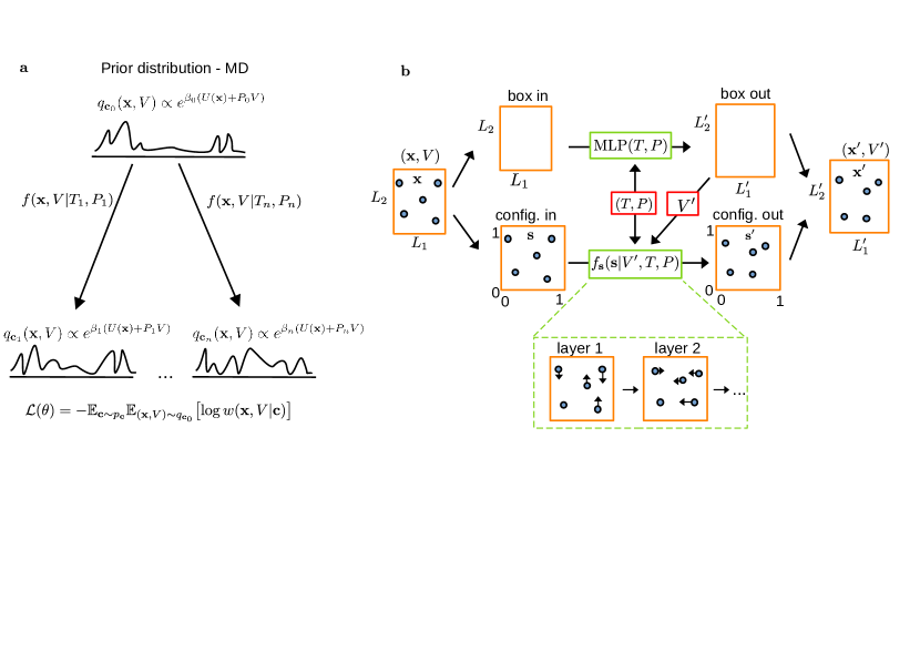
The key idea behind our approach is to compute free energy differences over a wide range of thermodynamic states without the need to run MD simulations at each state point. This is achieved by training a normalizing flow conditioned on temperature and pressure, which learns the mapping from a prior distribution at a reference thermodynamic state to a whole family of target distributions across thermodynamic space. Figure 1 a) illustrates the workflow of our approach. We first sample the prior distribution at the reference state in the ensemble with MD and save samples consisting of the atomic configuration and the box volume . In this work, we consider rectangular boxes and only allow for isotropic scaling, but the proposed approach is completely general and can easily be extended to fully triclinic simulation boxes. Samples from the prior distribution of the reference state with temperature and pressure are transformed by the flow to a generated configuration and volume in order to approximate equilibrium distributions at multiple different thermodynamic conditions. While the volume is updated using an affine transformation conditioned on the thermodynamic state, the configuration is first scaled to fractional coordinates and then transformed by a flow conditioned on the updated volume as well as on the thermodynamic state. For both transformations, the conditioning is achieved by feeding the thermodynamic state as an additional input to the model during training (Fig. 1 b) [25].
To optimize the flow parameters, we employ conditional energy-based training, avoiding the need to sample the target distributions. In particular, the average of the KL divergences between the generated and the target distributions conditioned on each target state over the entire range of thermodynamic states is evaluated, yielding the following loss function (see 4.2 for a derivation):
| (1) | ||||
Here, and denote the potential energy and inverse temperature, respectively. The conditioning states are drawn from the distribution , and is the sample generated by the conditional flow with parameters and Jacobian . After training, equilibrium expectation values of an observable can be computed as
| (2) |
using the conditional importance weights (Eq. (10)). Compared to temperature steerable flows [29], the proposed workflow is more general and allows for more flexible models, as no requirements need to be placed on the architecture or the prior.
The evaluation of Eq. (1) involves the average of the KL divergences over multiple thermodynamic target states. One option to choose these target states is to define a set of discrete points which are used throughout training [25, 27]. However, for conditioning points this results in times the number of energy evaluations per sample. In addition, the spacing between the points has to be small enough such that the flow is able to efficiently interpolate between them. We overcome these limitations by randomly drawing from a uniform distribution defined over the range of thermodynamic conditions of interest and transforming each sample with an individual -value. This approach is computationally more efficient and also allows to condition over a continuous range rather than for a fixed number points.
As condensed phase systems can exist in the liquid as well as in the solid phase, it is crucial to treat both phases on the same footing. We therefore build upon the coupling flow architecture originally proposed in Ref. 18 and refined in Refs. 19, 21 which allows to model ordered and disordered systems, such as solids and liquids, with the same architecture. Concretely, periodic boundary conditions can be respected utilizing circular splines [30], bijective transformations defined on a torus, whereas invariance under particle permutation can be achieved using (by construction) permutation-equivariant transformers [31] (see Sec. 4.3 for details).
2.2 Training efficiency of conditioned and single-point normalizing flows
The conditioning framework introduced in the previous section has the advantage that samples can be generated over a continuous range of thermodynamic conditions. It requires, however, to train a conditional flow which might converge slower than a single-point flow trained only for one specific temperature and pressure. To compare the convergence of the two flow types, we train both a conditional and single-point flow to transform samples of a 180 particle Lennard-Jones (LJ) face-centred cubic (FCC) crystal from a prior thermodynamic state at with (in reduced LJ units, see Supplementary Information (SI) for computational details). While the single-point flow is trained to generate samples of the equilibrium distribution at an evaluation point with , the conditional flow is trained to generate samples for and . Extensive statistics over the training process is collected by running 10 independent models (see SI for details).
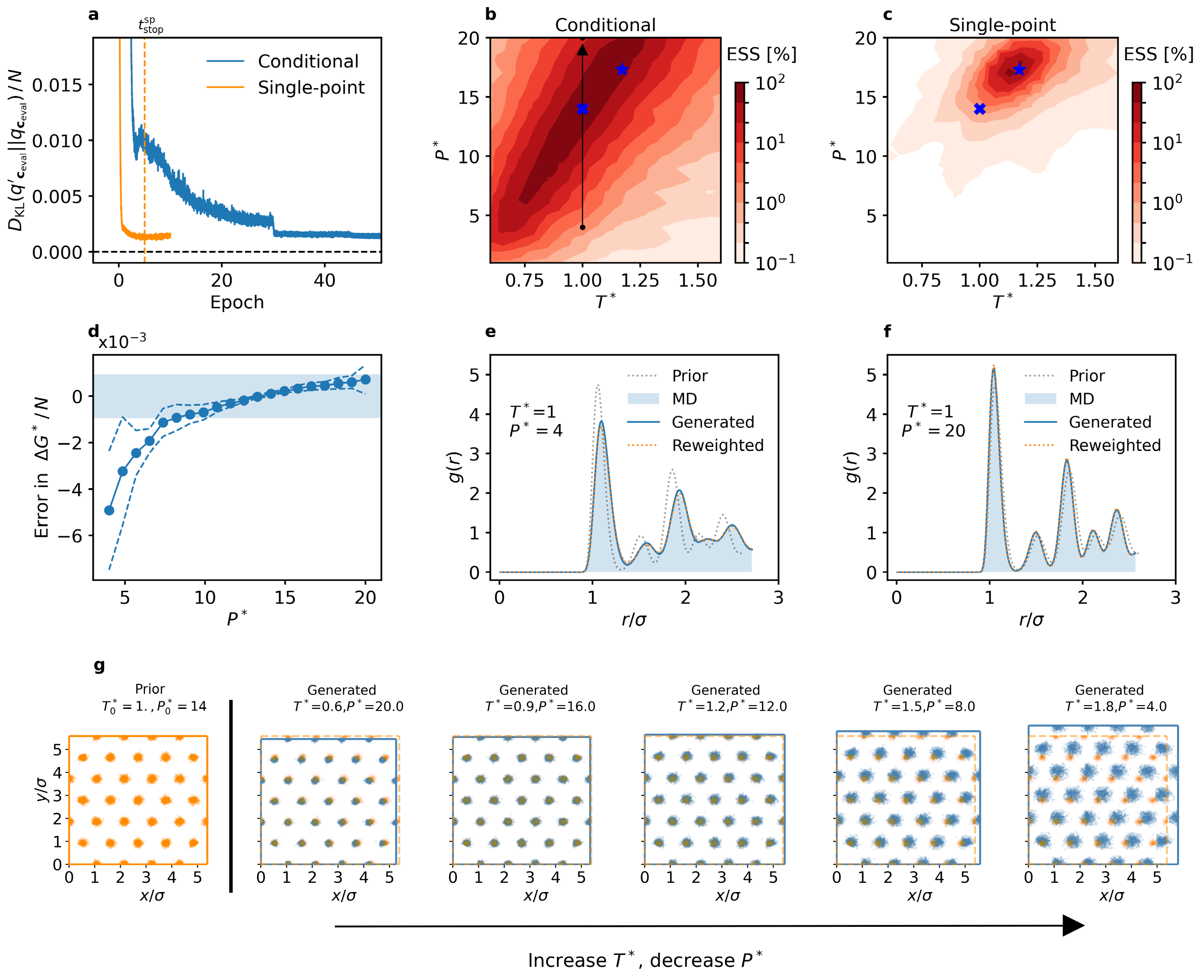
To measure the performances of the two flow types over training time, we evaluate the KL divergence (Eq. (12), with from standard MD+MBAR simulations) between the generated distribution and the target distribution at the evaluation point (Fig. 2 a). The KL divergence of the single-point flow quickly converges within a few epochs, after which an increase in divergence indicates the onset of overfitting. The KL divergence of the conditional flow is much more noisy in the first 20 epochs of training, with a temporary increase before continuing to decrease. The convergence behavior can be explained by the fact that the conditional flow requires more training steps as it learns a whole family of mappings simultaneously. After applying a learning rate reduction, becomes less noisy and converges to a similar value as the single-point flow. Even though training the conditional flow until convergence requires approximately 10 times more epochs than training the single-point flow, the additional training cost is amortized by the wide range of thermodynamic states covered by the conditional flow.
This becomes evident when comparing the statistical performance of the two flow types over the entire -range, which is evaluated using the effective sampling size (ESS) [32] (Eq. (11)). The ESS over the entire -range for the conditional and single-point flows is shown in Fig. 2 b and c, respectively. While the single-point flow reaches high efficiencies close to the evaluation point, the efficiency quickly decays and is close to zero for all other -conditions. In contrast, the conditional flow has a very high sampling efficiency of more than 60% over a wide range of thermodynamic states. We found that within LFEP already a few tens of effective samples are sufficient to obtain an accurate estimate of free energy differences. Within the regions of largest efficiencies, highly accurate free energy predictions can already be achieved evaluating only around 100 samples. Similarly, using 2 000 test samples, efficiencies as low as 1 % are sufficient to compute free energy differences with high accuracy. Remarkably, similar observations regarding sampling efficiency and free energy differences hold for the liquid phase, although the range of large sampling efficiencies was slightly smaller. For the corresponding efficiency map of the liquid, we refer to the SI.
The sampling efficiency in Fig. 2 b is almost constant along a diagonal line in crossing the prior state. This may reflect the fact that along this line the flow has to learn only a small transformation, as an increase in temperature leads to an increase in the atomic displacements and volume, whereas an increase in pressure has the opposite effect.
To assess the accuracy of the flow as free energy estimator, using 2 000 test samples, we compute the Gibbs free energy difference (Eq. (18)) with respect to the prior along the path for a fixed and evaluate the error compared to results obtained with MBAR used across a set of MD simulations (Fig. 2 d). Overall, we observe that both methods are in excellent agreement over the entire range. The accuracy only decreases slightly with increasing distance from the prior and decreasing sampling efficiency. Nevertheless, even for the furthest point, , the mean deviation per particle is only , while the absolute value in between and is around 14.5 per particle, that is the maximum relative error along the line is less than 0.05%. This demonstrates that the conditional flow can be used for the efficient evaluation of free energy differences also for states far away from the prior.
Furthermore, we illustrate the ability of the model to accurately capture pairwise correlations over varying thermodynamic conditions by computing the radial distribution function (RDF) [5] for configurations at the start and end point of the path (Fig. 2 e and f) and compare to MD. For both -conditions, the RDFs resulting from samples of the generated distributions are nearly indistinguishable from the MD results, even before reweighting, while samples from the prior distribution clearly yield different RDFs. Any remaining deviations between the mapped and MD results are resolved by reweighting the generated samples (Eq. (2)). The ability of the conditional flow model to generate samples with varying displacements and volumes is further illustrated in Fig. 2 g, where 2D-projections of 500 generated configurations with increasing temperature and decreasing pressure are shown.
2.3 Mapping out coexistence lines
Having demonstrated the efficiency of the conditional flow for accurately computing free energy differences over a wide range of thermodynamic states, we now apply this methodology to the exploration of the phase diagram of the LJ system.
Determining the coexistence line requires to find the thermodynamic states of equal free energy. As discussed in the introduction, this is a tedious and expensive task using traditional free energy estimators as a suitable set of discrete thermodynamic states needs to be identified and full MD/MC simulations, including potentially large equilibration times, need to be executed at each point [33]. In the case of liquid-solid coexistence lines, an additional complication arises from the fact that suitable states, in which both the solid and the liquid phase can be simulated and no phase transition occurs during the simulation time, need to be selected by hand.
Using the LJ system as an example, we demonstrate that our framework based on -conditioned flows can alleviate these issues. Specifically, we compute the coexistence line between the solid FCC and liquid phase. The only user-defined input to our workflow consists in choosing appropriate locations of the prior states for the two phases of interest. If a point of coexistence is already known, this point is a good choice as the sampling efficiency is highest close to the prior location (see Fig. 2) which allows to compute the coexistence line with only a small number of samples. To emphasize that our approach works without explicit knowledge of the coexistence region, we define a broad range of thermodynamic states with and in which the coexistence line is expected [34]. Based on physical intuition, we place the prior for the solid at low temperature and high pressure , and for the liquid at high temperature and low pressure . Conditional flows for both phases are trained over the expected region of coexistence (details are given in the SI). After training, we define a grid of points in the diagram with a spacing of =(0.05,1.4) and use the flows to evaluate the relative free energies to the respective prior based on 2000 samples.
To obtain the difference in free energy between the two phases, the absolute free energies at the prior locations are required. These are determined by evaluating the free energy difference to analytically or numerically tractable reference systems. For the solid phase, this could also be achieved using normalizing flows, as shown in Ref. 21. Here, we instead chose the more traditional and computationally more efficient approach of MBAR together with MD simulations. For the solid phase, the Einstein crystal [2] serves as a reference, while the liquid phase is connected to the Uhlenbeck-Ford model [35] (see Sec. 4.5 for details).
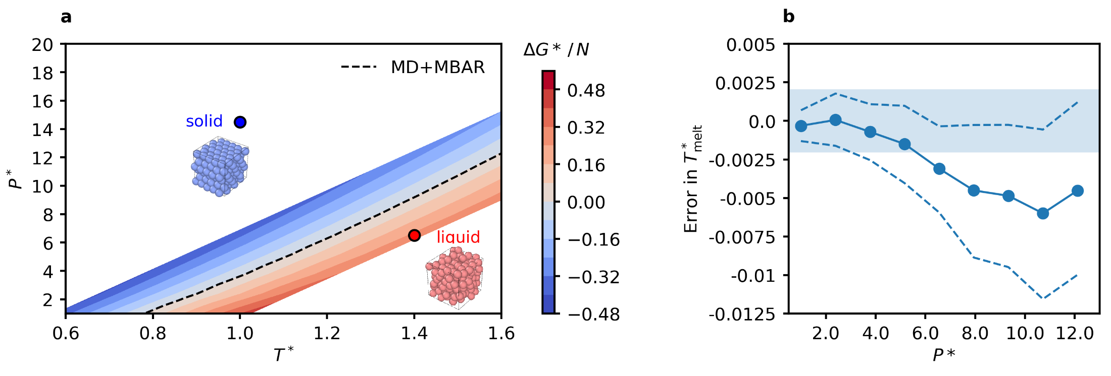
In Fig. 3 a, the free energy difference between the solid and liquid phase around the coexistence line is shown as a function of temperature and pressure (see SI for free energy differences over the entire -range considered during training). The coexistence line predicted by the flow is in excellent agreement with the reference values, obtained from high-accuracy MD+MBAR simulations (dashed line in Fig. 3 a), with only small deviations in the high-temperature region. In Fig. 3 b, the error in the melting temperatures as a function of pressure are shown as determined by the flow in comparison to MD+MBAR. For the low-pressure regions, the melting temperatures predicted by the flow are well within the error bars of the reference calculations. Only for higher pressures, deviations become slightly larger. Overall, the point of equal free energy, and therefore the melting temperatures, can be determined with a maximum (mean) deviation accuracy of less than .
2.4 Computational efficiency
A direct comparison of the computational costs for mapping out an entire phase diagram is not entirely straightforward as it depends on a variety of factors. Here, we focus on the number of required energy evaluations which will dominate our flow-based approach as well as traditional free energy estimators for more accurate and expensive interaction models, including ML potentials and ab initio approaches.
For MBAR, the number of energy evaluations is determined by the discretization of the -range and the number of samples needed for convergence at a given grid density. For the flow, generating a sufficient number of prior samples constitutes the main computational investment. The LJ solid in this study melts when the coexistence line is overstepped by around 0.1 or 1 . Consequently, the grid spacing for MBAR should be at maximum =(0.05 ,0.5) resulting in a total of 800 simulation points per phase. At this grid spacing, at least 100 MD samples per state separated by 500 decorrelation steps need to be collected for MBAR to converge the coexistence line with similar accuracy as the flow, where each MD simulation additionally requires at least 20 000 initial equilibration steps. In total, this amounts to 56 million energy evaluations per phase. For the chosen flow architecture, including more than 20 000 prior samples does not substantially improve the sampling efficiency. Generating these MD samples with the same number of decorrelation steps requires around 10 million energy evaluations, while training for 50 epochs adds less than one million. The final evaluation of 2000 samples on the grid of 800 points adds 1.6 million energy evaluations. Within this rough estimate, the number of required energy evaluation is already reduced by a factor of 5 for the system presented here. In addition, flow-based generation of samples does not require the evaluation of forces which, for expensive potentials, constitutes an additional advantage.
3 Discussion
The introduced framework based on conditional normalizing flows provides a novel approach to efficiently calculate differences in free energies over a wide range of thermodynamic states. Contrary to traditional approaches, such as thermodynamic integration or expanded ensembles, it does not require an explicit discretization of the temperature and pressure space. For both solid and liquid phases, flows trained in a conditional fashion achieve large sampling efficiencies even far away from the prior states. As a consequence, only minimal prior knowledge about the system and the melting region is required to map out coexistence lines between two phases with high accuracy. Our workflow, therefore, constitutes a first step towards the efficient and simple calculation of phase diagrams using normalizing flows.
The combination of MD prior data with normalizing flows and the subsequent connection to tractable reference systems allows to compute -dependent absolute free energies of the solid phase much more efficiently than purely flow-based approaches [19, 21]. In addition, our approach is equally applicable to evaluate absolute free energies of the liquid phase which is currently out of reach with purely flow-based methods [36]. Nevertheless, the connection to the tractable reference systems remains computationally expensive. As a next step, a flow-based framework to directly compute free energy differences between phases, ideally utilizing the prior samples of the two phases, would be desirable.
A second direction concerns the system sizes which can be tackled with our approach. In our studies as well as in previous research [37], it was found that the sampling efficiency decreases significantly with increasing system sizes. For the application to realistic systems, thousands of atoms may be required to accurately reproduce experimental results which is unfeasible using current flow-based sampling methodologies. A possible solution could consist in training a transferable model on small systems that can then efficiently be applied to larger ones. With an increase in sampling efficiency, the application of our approach to more accurate potentials as well as the inclusion of molecular crystals [38] becomes feasible and is planned in future work. By advancing the aforementioned fields, we aim to improve the utility and applicability of our approach to enhance the understanding of complex phase behaviour in realistic systems.
4 Methods
4.1 Traditional free energy estimators
We consider the isothermal-isobaric () ensembles, for which the reduced potential of a configuration is defined as [4]
| (3) |
where is the potential energy, is the volume of the simulation box at configuration , and denotes the inverse temperature. The reduced potential defines the equilibrium distribution
| (4) |
where is the configurational partition function given by the integral over the configuration space .
From the partition function, the dimensionless configurational free energy can be obtained as
| (5) |
Since evaluating the integral over configuration space is unfeasible for most interaction potentials, evaluating the absolute free energy is usually impossible. A more tractable approach is to evaluate the difference in free energy between two states and , , as
| (6) |
with the difference in the reduced potential . Eq. (6) is known as Zwanzig identity [3], which is a central result of Free Energy Perturbation (FEP) and constitutes the foundation of many free energy estimators. While being formally exact, the convergence of FEP crucially depends on the overlap between the corresponding configurational distributions and , making it a highly biased and noisy estimator in practical calculations, even for small molecules [39].
A statistically more optimal estimator can be obtained using samples from both states of interest as done in the Bennett Acceptance Ratio (BAR) and its multistate extension MBAR [4]. Nevertheless, the overlap problem remains which is commonly solved by defining a sequence of intermediate Hamiltonians between the two states of interest. However, such multi-staged approaches require samples from all intermediate states and it is not clear how best to define the intermediate stages.
Targeted free energy perturbation (TFEP) [6] tackles the problem of having intermediate states by defining an invertible map transforming samples from to samples from a new target distribution which shares a larger overlap with than . For a perfect map, . Similarly, the inverse map transforms samples from to and for a perfect map. Using the Jacobian of the mapping, , the generated distribution can be computed analytically using the change of variable theorem
| (7) |
Samples drawn from the generated distribution can be reweighted to the target distribution by assigning a statistical weight , which can be computed using various algorithms [40]. Here, we follow Ref. 13 and define the importance weights of the generated samples as
| (8) |
The dimensionless free energy difference between and can then be obtained as
| (9) |
For the probability distributions of interest (Eq. (4)), the importance weights are given by
| (10) | ||||
The weights can further be utilized to evaluate how well the learned distribution approximates the target distribution through the Kish effective sample size (ESS) [32]
| (11) |
The ESS provides a rough measure for how many uncorrelated samples would result in a Monte-Carlo estimator of the same statistical performance (typically reported relative to the total number of generated samples).
4.2 Conditioning normalizing flows on temperature and pressure
Normalizing flows are a class of deep generative models which are able to generate samples from a target distribution [14, 42]. Normalizing flows aim to learn the optimal set of parameters of an invertible function that maps samples from a prior distribution into samples from a target distribution . In practice, the learned set of parameters will be different from and the flow is trained to minimize the Kullback-Leibler (KL) divergence between the generated distribution and . For physical systems with an equilbirium distribution defined in Eq. (4), the KL divergence can be expressed as [13, 18]:
| (12) |
where the importance weights are defined similarly to Eq. (8) and is the free energy difference between and . Since is independent of the trainable weights, the loss function simplifies to
| (13) |
For efficient training, the determinant of the Jacobian of the transformation must be easy to calculate (see Eq. (8)). For this purpose, coupling layers [43, 44] were designed which split the input data into two channels and transform one of the channels conditioned on the other. This yields a triangular Jacobian whose determinant can be evaluated analytically. The entire input vector can be transformed by stacking several coupling layers, whereby the channel to be transformed changes.
A conditional normalizing flow can be trained to learn a mapping between a prior distribution and a conditional target distribution for a vector of conditioning variables [25, 26]. In this case, the change of variable reads
| (14) |
For energy-based training, the trainable parts of the conditional KL divergence are given by [25, 27]
| (15) |
with the conditional importance weights defined as . In Eq. (15), we used the single-point loss from Eq. (13) and defines the distribution of the conditional variable. In practice, conditioning a coupling flow architecture can be easily achieved by concatenating the conditioning variable to the unchanged part before transforming the other part [25].
For the application to free energy sampling within TFEP in the isobaric-isothermal () ensemble, we aim to train a normalizing flow to learn a mapping conditioned on temperature and pressure () between equilibrium distributions of the form (see Eq. (3))
| (16) |
For brevity, we use in the following. In this notation, we want to learn a mapping between a prior distribution , sampled with MD, and the conditional target distribution . For training the flow, we minimize the conditional loss function (Eq. (15)) using the importance weights defined in Eq. (10):
| (17) |
which results in the loss function Eq. (1). Once the flow is trained, the free energy difference between the prior distribution and the target distribution is obtained from TFEP (Eq. (9))
| (18) |
4.3 Flow architecture
As sketched in Fig. 1, our flow is based on a shape-conditional architecture [21]. Here, the volume is updated by an affine transformation, while the atomic configurations are first scaled to fractional coordinates and then updated conditioned on the volume and the thermodynamic state.
Our flow transforms a sample of the prior distribution to , where the volume is connected to the box dimensions by . In this work, we focus on the simulation of solids and liquids and therefore apply certain restrictions regarding the shape of the simulation box. We use orthorhombic simulation boxes with and further only allow for an isotropic scaling of the box (), such that the box is fully characterized by its volume .
The volume transformation and the transformation of the position of particle can be written as
| (19) | ||||
| (20) | ||||
| (21) | ||||
| (22) |
Here, and are the output of a multilayer perceptron taking as input pressure and temperature, where is bounded below by -1. and denote element-wise multiplication and division, respectively. The transformed box dimensions are given by . is the output for particle of a -conditional coupling flow over configurations (see following paragraph for details), operating on fractional coordinates. After the transformation, are transformed to physical coordinates by multiplying with the new box lengths.
The procedure just described gives rise to three contributions to the Jacobian, , , and . arises from Eq. (19) and is given by . accounts for the initial global scaling of the coordinates to fractional coordinates and the final scaling of the flow output to physical coordinates (Eqs. (20) and (22)) and is given by . Finally, accounts for the transformation in Eq. (21) and can be obtained from .
4.4 Conditional coupling layer
To be applicable to condensed phase system, must respect periodic boundary conditions and invariance under particle permutation. In addition, the center of mass needs to be fixed to prevent uncontrolled errors in the free energy prediction due to rigid translations [20].
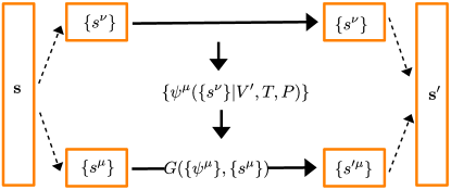
To achieve these requirements, we extend the coupling layer originally proposed in [18] and refined in [19] to the case of conditional sampling. Figure 4 shows our implementation of a conditional coupling layer. The -particle configuration is split over cartesian coordinates into two subsets and , e.g. . First, all coordinates indexed by remain unchanged while the coordinates of atom carrying index are transformed according to
| (23) |
with
| (24) |
Here, is a circular spline [30], which naturally accounts for the periodicity of the problem. The parameters of the spline are obtained as the output of a transformer [31] for the coordinates indexed by of particle , which takes as input circular encodings of the coordinates and is conditioned on ,, and . The partitioning of and is changed between layers such that each coordinate gets transformed (see [18, 19] for details).
The invariance of the target density with respect to particle permutation is ensured due to permutation-equivariance of the transformer update [45]. In order to prevent the flow from learning a global shift, we fix one of the atoms and transform the coordinates of the remaining particles.
4.5 Computing coexistence lines
The coexistence line in the diagram of two phases of a system is defined by equal total Gibbs free energies including the kinetic contribution. For a given state (), is the sum of the configurational contribution (Eq. (5)) and the kinetic contribution:
| (25) |
Here, is the thermal De-Broglie wavelength .
For each phase, the configurational contribution can be obtained by combining relative differences within phases with the absolute free energy at a reference state .) Using the difference in the dimensionless free energy between the reference point and a state , , and writing it explicitly as
| (26) |
the absolute Gibbs free energy can be obtained as
| (27) |
The differences can be obtained from free energy estimators such as MBAR and TFEP (Eq. (9)) after performing simulations of the physical system.
is not directly available from simulations of the system of interest. Instead, it can be obtained by connecting the physical system to a model system whose Helmholtz free energy at the reference point, with , can be computed analytically. Then, the reference free energy can be computed as
| (28) |
with being the difference in Helmholtz free energy between the model and the physical system at the reference temperature. This quantity can be computed defining a set of intermediate Hamiltonians between physical and model system for which MD simulations are performed. The resulting energy histograms serve as input for MBAR. In this work, we use as reference systems for the solid and the liquid phase the Einstein crystal [5] and the Uhlenbeck-Ford (UF) model [35], respectively (see SI for details).
In principle, a flow can be used to determine as well as . However, it has been shown that obtaining is computationally much more expensive than an MD+MBAR based approach [19]. For a flow-based calculation of the coexistence line, we therefore decide to determine using MD+MBAR and to use our conditional flow approach to obtain .
Code availability
The flow models developed in this work are available on GitHub at https://github.com/maxschebek/flow_diagrams. Models were built and trained using JAX [46], equinox [47], and jax-md [48].
References
- \bibcommenthead
- Chew and Reinhardt [2023] Chew, P.Y., Reinhardt, A.: Phase diagrams—Why they matter and how to predict them. J. Chem. Phys. 158(3), 030902 (2023) https://doi.org/10.1063/5.0131028
- Vega et al. [2008] Vega, C., Sanz, E., Abascal, J.L.F., Noya, E.G.: Determination of phase diagrams via computer simulation: methodology and applications to water, electrolytes and proteins. J. Phys. Condensed Matter 20(15), 153101 (2008) https://doi.org/10.1088/0953-8984/20/15/153101
- Zwanzig [2004] Zwanzig, R.W.: High‐Temperature Equation of State by a Perturbation Method. I. Nonpolar Gases. J. Chem. Phys. 22(8), 1420–1426 (2004) https://doi.org/10.1063/1.1740409
- Shirts and Chodera [2008] Shirts, M.R., Chodera, J.D.: Statistically optimal analysis of samples from multiple equilibrium states. J. Chem. Phys. 129(12), 124105 (2008) https://doi.org/10.1063/1.2978177
- Frenkel and Smit [2002] Frenkel, D., Smit, B.: Understanding Molecular Simulation: From Algorithms to Applications, 2nd edn. Computational Science Series, vol. 1. Academic Press, San Diego (2002)
- Jarzynski [2002] Jarzynski, C.: Targeted free energy perturbation. Phys. Rev. E 65, 046122 (2002) https://doi.org/10.1103/PhysRevE.65.046122
- Schieber and Shirts [2019] Schieber, N.P., Shirts, M.R.: Configurational mapping significantly increases the efficiency of solid-solid phase coexistence calculations via molecular dynamics: Determining the FCC-HCP coexistence line of Lennard-Jones particles. J. Chem. Phys. 150(16), 164112 (2019) https://doi.org/10.1063/1.5080431
- Schütt et al. [2018] Schütt, K.T., Sauceda, H.E., Kindermans, P.-J., Tkatchenko, A., Müller, K.-R.: SchNet – A deep learning architecture for molecules and materials. J. Chem. Phys. 148(24), 241722 (2018) https://doi.org/10.1063/1.5019779
- Batzner et al. [2022] Batzner, S., Musaelian, A., Sun, L., Geiger, M., Mailoa, J.P., Kornbluth, M., Molinari, N., Smidt, T.E., Kozinsky, B.: E(3)-equivariant graph neural networks for data-efficient and accurate interatomic potentials. Nature Communications 13(1) (2022) https://doi.org/10.1038/s41467-022-29939-5
- Zhang et al. [2018] Zhang, L., Han, J., Wang, H., Car, R., E, W.: Deep potential molecular dynamics: A scalable model with the accuracy of quantum mechanics. Phys. Rev. Lett. 120, 143001 (2018) https://doi.org/10.1103/PhysRevLett.120.143001
- Niu et al. [2020] Niu, H., Bonati, L., Piaggi, P.M., Parrinello, M.: Ab initio phase diagram and nucleation of gallium. Nat. Commun. 11(1), 2654 (2020) https://doi.org/10.1038/s41467-020-16372-9
- Zhang et al. [2021] Zhang, L., Wang, H., Car, R., E, W.: Phase diagram of a deep potential water model. Phys. Rev. Lett. 126, 236001 (2021) https://doi.org/10.1103/PhysRevLett.126.236001
- Noé et al. [2019] Noé, F., Olsson, S., Köhler, J., Wu, H.: Boltzmann generators: Sampling equilibrium states of many-body systems with deep learning. Science 365(6457) (2019) https://doi.org/10.1126/science.aaw1147
- Tabak and Vanden-Eijnden [2010] Tabak, E., Vanden-Eijnden, E.: Density estimation by dual ascent of the log-likelihood. Communications in Mathematical Sciences 8(1), 217–233 (2010) https://doi.org/10.4310/CMS.2010.v8.n1.a11
- Rezende and Mohamed [2015] Rezende, D.J., Mohamed, S.: Variational inference with normalizing flows. In: Proceedings of the 32nd International Conference on International Conference on Machine Learning - Volume 37. ICML’15, pp. 1530–1538 (2015). https://arxiv.org/abs/1505.05770
- Albergo et al. [2019] Albergo, M.S., Kanwar, G., Shanahan, P.E.: Flow-based generative models for markov chain monte carlo in lattice field theory. Phys. Rev. D 100, 034515 (2019) https://doi.org/10.1103/PhysRevD.100.034515
- Nicoli et al. [2021] Nicoli, K.A., Anders, C.J., Funcke, L., Hartung, T., Jansen, K., Kessel, P., Nakajima, S., Stornati, P.: Estimation of thermodynamic observables in lattice field theories with deep generative models. Phys. Rev. Lett. 126, 032001 (2021) https://doi.org/10.1103/PhysRevLett.126.032001
- Wirnsberger et al. [2020] Wirnsberger, P., Ballard, A.J., Papamakarios, G., Abercrombie, S., Racanière, S., Pritzel, A., Jimenez Rezende, D., Blundell, C.: Targeted free energy estimation via learned mappings. J. Chem. Phys. 153(14), 144112 (2020) https://doi.org/%****␣article.bbl␣Line␣325␣****10.1063/5.0018903
- Wirnsberger et al. [2022] Wirnsberger, P., Papamakarios, G., Ibarz, B., Racanière, S., Ballard, A.J., Pritzel, A., Blundell, C.: Normalizing flows for atomic solids. Mach. Learn. Sci. Technol. 3(2), 025009 (2022) https://doi.org/10.1088/2632-2153/ac6b16
- Ahmad and Cai [2022] Ahmad, R., Cai, W.: Free energy calculation of crystalline solids using normalizing flows. Model. Simul. Mat. Sci. Eng. 30(6), 065007 (2022) https://doi.org/10.1088/1361-651X/ac7f4b
- Wirnsberger et al. [2023] Wirnsberger, P., Ibarz, B., Papamakarios, G.: Estimating gibbs free energies via isobaric-isothermal flows. Mach. Learn. Sci. Technol. 4(3), 035039 (2023) https://doi.org/10.1088/2632-2153/acefa8
- van Leeuwen et al. [2023] Leeuwen, S., Ortíz, A.P.d.A., Dijkstra, M.: A Boltzmann generator for the isobaric-isothermal ensemble (2023) https://doi.org/10.48550/arXiv.2305.08483
- Rizzi et al. [2023] Rizzi, A., Carloni, P., Parrinello, M.: Free energies at qm accuracy from force fields via multimap targeted estimation. Proceedings of the National Academy of Sciences 120(46), 2304308120 (2023) https://doi.org/%****␣article.bbl␣Line␣400␣****10.1073/pnas.2304308120
- Invernizzi et al. [2022] Invernizzi, M., Krämer, A., Clementi, C., Noé, F.: Skipping the replica exchange ladder with normalizing flows. J. Phys. Chem. Lett. 13(50), 11643–11649 (2022) https://doi.org/10.1021/acs.jpclett.2c03327
- Ardizzone et al. [2019] Ardizzone, L., Lüth, C., Kruse, J., Rother, C., Köthe, U.: Guided Image Generation with Conditional Invertible Neural Networks (2019). https://doi.org/10.48550/arXiv.1907.02392
- Winkler et al. [2019] Winkler, C., Worrall, D., Hoogeboom, E., Welling, M.: Learning Likelihoods with Conditional Normalizing Flows (2019). https://doi.org/10.48550/arXiv.1912.00042
- Falkner et al. [2023] Falkner, S., Coretti, A., Romano, S., Geissler, P.L., Dellago, C.: Conditioning boltzmann generators for rare event sampling. Mach. Learn. Sci. Technol. 4(3), 035050 (2023) https://doi.org/10.1088/2632-2153/acf55c
- Gerdes et al. [2023] Gerdes, M., Haan, P., Rainone, C., Bondesan, R., Cheng, M.C.N.: Learning lattice quantum field theories with equivariant continuous flows. SciPost Phys. 15, 238 (2023) https://doi.org/10.21468/SciPostPhys.15.6.238
- Dibak et al. [2021] Dibak, M., Klein, L., Krämer, A., Noé, F.: Temperature Steerable Flows and Boltzmann Generators. Phys. Rev. Res. 4(4), 042005 (2021) https://doi.org/10.1103/PhysRevResearch.4.L042005
- Rezende et al. [2020] Rezende, D.J., Papamakarios, G., Racaniere, S., Albergo, M., Kanwar, G., Shanahan, P., Cranmer, K.: Normalizing flows on tori and spheres. In: III, H.D., Singh, A. (eds.) Proceedings of the 37th International Conference on Machine Learning. Proceedings of Machine Learning Research, vol. 119, pp. 8083–8092 (2020). https://doi.org/10.48550/arXiv.2002.02428
- Vaswani et al. [2017] Vaswani, A., Shazeer, N., Parmar, N., Uszkoreit, J., Jones, L., Gomez, A.N., Kaiser, L., Polosukhin, I.: Attention is all you need. In: Proceedings of the 31st International Conference on Neural Information Processing Systems, pp. 6000–6010 (2017). https://doi.org/10.48550/arXiv.1706.03762
- Kish [1965] Kish, L.: Sampling organizations and groups of unequal sizes. Am. Sociol. Rev. 30(4), 564–572 (1965)
- [33] A simple method for automated equilibration detection in molecular simulations. J. Chem. Theory Comput. 12(4), 1799–1805 (2016) https://doi.org/10.1021/acs.jctc.5b00784
- Bizjak et al. [2009] Bizjak, A., Urbič, T., Vlachy, V.: Phase diagram of the lennard-jones system of particles from the cell model and thermodynamic perturbation theory. Acta Chim. Slov. 56, 166–171 (2009)
- Paula Leite et al. [2016] Paula Leite, R., Freitas, R., Azevedo, R., Koning, M.: The uhlenbeck-ford model: Exact virial coefficients and application as a reference system in fluid-phase free-energy calculations. J. Chem. Phys. 145(19) (2016) https://doi.org/10.1063/1.4967775
- Coretti et al. [2022] Coretti, A., Falkner, S., Geissler, P., Dellago, C.: Learning Mappings between Equilibrium States of Liquid Systems Using Normalizing Flows (2022) https://doi.org/%****␣article.bbl␣Line␣600␣****10.48550/arXiv.2208.10420
- Abbott et al. [2022] Abbott, R., Albergo, M.S., Botev, A., Boyda, D., Cranmer, K., Hackett, D.C., Matthews, A.G.D.G., Racanière, S., Razavi, A., Rezende, D.J., Romero-López, F., Shanahan, P.E., Urban, J.M.: Aspects of scaling and scalability for flow-based sampling of lattice QCD (2022) https://doi.org/10.48550/arXiv.2211.07541
- Köhler et al. [2023] Köhler, J., Invernizzi, M., De Haan, P., Noé, F.: Rigid body flows for sampling molecular crystal structures. In: Proceedings of the 40th International Conference on Machine Learning. Proceedings of Machine Learning Research, vol. 202, pp. 17301–17326 (2023). https://proceedings.mlr.press/v202/kohler23a.html
- Mey et al. [2020] Mey, A.S.J.S., Allen, B.K., Bruce McDonald, H.E., Chodera, J.D., Hahn, D.F., Kuhn, M., Michel, J., Mobley, D.L., Naden, L.N., Prasad, S., Rizzi, A., Scheen, J., Shirts, M.R., Tresadern, G., Xu, H.: Best practices for alchemical free energy calculations. Living J. Comp. Mol. Sci. 2(1), 18378 (2020) https://doi.org/10.33011/livecoms.2.1.18378
- Olehnovics et al. [2024] Olehnovics, E., Liu, Y.M., Mehio, N., Sheikh, A.Y., Shirts, M., Salvalaglio, M.: Assessing the accuracy and efficiency of free energy differences obtained from reweighted flow-based probabilistic generative models (2024) https://doi.org/10.26434/chemrxiv-2024-z9g39
- Rizzi et al. [2021] Rizzi, A., Carloni, P., Parrinello, M.: Targeted free energy perturbation revisited: Accurate free energies from mapped reference potentials. J. Phys. Chem. Lett. 12(39), 9449–9454 (2021) https://doi.org/10.1021/acs.jpclett.1c02135
- Papamakarios et al. [2021] Papamakarios, G., Nalisnick, E., Rezende, D.J., Mohamed, S., Lakshminarayanan, B.: Normalizing flows for probabilistic modeling and inference. J. Mach. Learn. Res. 22(1) (2021) http://jmlr.org/papers/v22/19-1028.html
- Dinh et al. [2014] Dinh, L., Krueger, D., Bengio, Y.: Nice: Non-linear independent components estimation (2014). https://arxiv.org/abs/1410.8516
- Dinh et al. [2017] Dinh, L., Sohl-Dickstein, J., Bengio, S.: Density estimation using real NVP. In: International Conference on Learning Representations (2017). https://arxiv.org/abs/1605.08803
- Köhler et al. [2020] Köhler, J., Klein, L., Noe, F.: Equivariant flows: Exact likelihood generative learning for symmetric densities. In: III, H.D., Singh, A. (eds.) Proceedings of the 37th International Conference on Machine Learning. Proceedings of Machine Learning Research, vol. 119, pp. 5361–5370 (2020). https://proceedings.mlr.press/v119/kohler20a.html
- Bradbury et al. [2018] Bradbury, J., Frostig, R., Hawkins, P., Johnson, M.J., Leary, C., Maclaurin, D., Necula, G., Paszke, A., VanderPlas, J., Wanderman-Milne, S., Zhang, Q.: JAX: Composable Transformations of Python+NumPy programs
- Kidger and Garcia [2021] Kidger, P., Garcia, C.: Equinox: neural networks in JAX via callable PyTrees and filtered transformations. Differentiable Programming workshop at Neural Information Processing Systems 2021 (2021) https://doi.org/10.48550/arXiv.2111.00254
- Schoenholz and Cubuk [2020] Schoenholz, S.S., Cubuk, E.D.: JAX M.D.: A framework for differentiable physics. In: Advances in Neural Information Processing Systems, vol. 33 (2020). https://papers.nips.cc/paper/2020/file/83d3d4b6c9579515e1679aca8cbc8033-Paper.pdf
Acknowledgements
MS and JR acknowledge financial support from Deutsche Forschungsgemeinschaft (DFG) through grant CRC 1114 \ldqScaling Cascades in Complex Systems\rdq, Project Number 235221301, Project B08 \ldqMultiscale Boltzmann Generators\rdq. JR acknowledges financial support from DFG through the Heisenberg Programme project 428315600. MI acknowledges support from the Humboldt Foundation for a Postdoctoral Research Fellowship. We thank Leon Klein for insightful discussions.