Entanglement swapping in critical quantum spin chains

Abstract

The transfer of quantum information between many-qubit states is a subject of fundamental importance in quantum science and technology. We consider entanglement swapping in critical quantum spin chains, where the entanglement between the two chains is induced solely by the Bell-state measurements. We employ a boundary conformal field theory (CFT) approach and describe the measurements as conformal boundary conditions in the replicated field theory. We show that the swapped entanglement exhibits a logarithmic scaling, whose coefficient takes a universal value determined by the scaling dimension of the boundary condition changing operator. We apply our framework to the critical spin-$\frac{1}{2}$ XXZ chain and determine the universal coefficient by the boundary CFT analysis. We also numerically verify these results by the tensor-network calculations. Possible experimental relevance to Rydberg atom arrays is briefly discussed.

Quantum information transfer and teleportation are central themes in quantum science and technology [1, 2]. One of the key concepts there is entanglement swapping, a process that entangles two systems solely by quantum measurements [3, 4, 5, 6, 7, 8, 9, 10, 11, 12, 13, 14]. After two decades from its first realization [15], recent advances [16, 17, 18, 19, 20] have now enabled quantum information transfer over distances exceeding $1000$ km with high fidelity [21, 22], showing great promise for realizing quantum cryptography [23] and quantum networks [24, 25, 26, 27].

Transfer of quantum information has also been an intriguing theoretical subject, dating back to the pioneering works on the Bell inequality [28] and the Lieb-Robinson bound [29]. An early study [4] has highlighted the possible advantage of entanglement swapping in multiparticle setups, and subsequent studies have explored the potential of using many-body systems for quantum information transfer [30, 31, 32, 33, 34]. From a broader perspective, previous studies have revealed various aspects of many-body states subject to measurement backaction; examples include measurement-induced phase transitions in quantum circuits [35, 36, 37, 38, 39, 40, 41, 42, 43, 44] and monitored fermions/bosons [45, 46, 47, 48, 49, 50, 51, 52, 53, 54, 55, 56, 57, 58], long-range entangled state preparation [59, 60, 61, 62, 63, 64, 65], measurement-enhanced entanglement [66, 67, 68, 69], and critical states under measurements or decoherence [70, 71, 72, 73, 74, 75, 76, 77, 78, 79, 80, 81, 82, 83, 84, 85, 86, 87]. In particular, it has been demonstrated in Refs. [79, 80, 81, 82, 83, 84, 85, 86, 87] that the effects of measurements on critical spin chains can be described by using the boundary conformal field theory (CFT) approach [88, 89, 90, 91, 92].

Despite these remarkable developments, our understanding of how measurements enable quantum information transfer between many-body states is still in its infancy. Quantum critical states are particularly interesting in this context since they possess large entanglement originating from long-range correlations [93]. Motivated by this, we consider entanglement swapping in critical quantum spin chains. There, the entanglement between the chains occurs without direct interactions but with measurements, and a number of fundamental questions arise. Does the swapped entanglement exhibit universality, and if yes, in what sense? How does it depend on the number of measured qubits? These questions are directly relevant to recent experiments realizing measurement and control of many-body systems at the single-quantum level [94, 95, 96, 97]. While the related questions have been recently addressed in Refs. [66, 33], theoretical understandings of quantum information transfer between critical chains induced solely by measurements are still lacking.

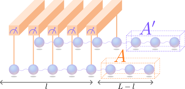
Figure 1: Schematic illustration of the setup. The initial state is a pair of independent identical critical ground states. The Bell-state measurements are performed on $l$ qubit pairs, rendering the unmeasured parts $A$ and $A^{\prime}$ entangled.

To address the above questions, we utilize a boundary CFT description and show that the swapped entanglement exhibits the universal logarithmic scaling as a function of the number of measured qubits. We point out that the Bell-state measurements can impose certain conformal boundary conditions on the time slice of the replicated CFT, leading to the universal coefficient determined by the scaling dimension of the boundary condition changing operator (BCCO). As a concrete example, we study the critical spin-$\frac{1}{2}$ XXZ chain described by the Tomonaga-Luttinger liquid (TLL) [98, 99] and determine the universal coefficient by the boundary CFT analysis. We numerically verify the field-theoretical results using the tensor-network calculations and discuss possible experimental relevance to Rydberg atom arrays.

Entanglement swapping in critical spin chains.— We consider two initially separable critical spin chains under periodic boundary conditions. Each of the chains consists of $L$ qubits labeled by $j,j^{\prime}{\in}\{1,2,{\ldots},L\}$ and is initially in the same critical ground state $\ket{\Psi_{0}}$. The entanglement swapping is achieved by performing the interchain Bell-state measurements (Fig. 1). Namely, two qubits across the initially independent chains are measured in the Bell basis, $\ket*{\mathrm{Bell}^{b_{1}b_{2}}}{=}(\ket*{0b_{1}}{+}(-1)^{b_{2}}\ket*{1\overline{b}_{1}})/\sqrt{2}$, which is labeled by the four binary numbers $b_{1}b_{2}\,{\in}\,\{0,1\}^{\otimes 2}$. The projection operator on the Bell basis in qubits $j,j^{\prime}$ is denoted by $P^{b_{1}b_{2}}_{jj^{\prime}}{=}|\mathrm{Bell}^{b_{1}b_{2}}_{jj^{\prime}}\rangle\langle\mathrm{Bell}^{b_{1}b_{2}}_{jj^{\prime}}|$. After obtaining measurement outcomes $\vec{m}\,{=}\,(m_{1},m_{2},\ldots,m_{l})\;(m_{j}\,{\in}\,\quantity{0,1}^{\otimes 2})$, the post-measurement state becomes

$$\ket*{\Psi^{\vec{m}}}=\frac{P^{\vec{m}}\ket*{\Psi_{0}}\!\otimes\!\ket*{\Psi_{0}}}{\sqrt{p_{\vec{m}}}}=\Biggl{[}\bigotimes_{j=j^{\prime}=1}^{l}\!\ket*{\mathrm{Bell}^{m_{j}}_{jj^{\prime}}}\Biggr{]}\otimes\!\ket*{\Psi^{\vec{m}}_{AA^{\prime}}},$$ (1)

where $P^{\vec{m}}=\prod_{j=j^{\prime}=1}^{l}P_{jj^{\prime}}^{m_{j}}$ is the projection operator corresponding to the outcome $\vec{m}$, $p_{\vec{m}}\,{=}\,\|P^{\vec{m}}\ket*{\Psi_{0}}\!\otimes\!\ket*{\Psi_{0}}\|^{2}$ is the Born probability, and the unmeasured region in each chain is denoted by $A,A^{\prime}$, respectively (cf. Fig. 1). The second expression in Eq. (1) follows from the fact that the projective measurements separate the measured qubits from the rest, rendering the unmeasured part a pure state $\ket{\Psi^{\vec{m}}_{AA^{\prime}}}$.

The key point is that the post-measurement state $\ket{\Psi^{\vec{m}}_{AA^{\prime}}}$ now possesses the interchain entanglement between $A$ and $A^{\prime}$, which is generated solely by the measurement. This measurement-induced entanglement, which we refer to as the swapped entanglement, can be quantified by the following entanglement entropy (EE),

$$S^{\vec{m}}_{A}=-\Tr[\rho^{\vec{m}}_{A}\ln\rho^{\vec{m}}_{A}],$$ (2)

where $\rho_{A}^{\vec{m}}\,{=}\,\Tr_{A^{\prime}}[\outerproduct*{\Psi^{\vec{m}}_{AA^{\prime}}}{\Psi^{\vec{m}}_{AA^{\prime}}}]$ is the reduced density matrix on $A$. For the sake of later convenience, we write $S^{\vec{m}}_{A}\,{=}\,S^{\vec{\mu}}_{A}$ in the case of uniform measurement outcomes where the outcomes for all the pairs coincide, i.e., $\vec{m}\,{=}\,\vec{\mu}\,{=}\,(\mu,\ldots,\mu)\;(\mu\,{\in}\,\{0,1\}^{\otimes 2})$. While $S^{\vec{m}}_{A}$ describes the entanglement properties specific to a measurement outcome $\vec{m}$, we will also analyze the following averaged EE as a quantity representing the typical behavior of the swapped entanglement:

$$\overline{S}_{A}=\sum_{\vec{m}}p_{\vec{m}}S^{\vec{m}}_{A}.$$ (3)

General field-theoretical approach.— The universality in the swapped entanglement can be understood by developing the CFT approach to the present problem. To this end, we employ the Euclidean path-integral representation and express the two spin chains by a two-component ($1{+}1$)-dimensional field $\bm{\phi}\,{=}\,(\phi,\phi^{\prime})$. The Euclidean action $\mathcal{S}[\bm{\phi}]$ in the bulk is simply the sum of CFT for each field. Meanwhile, the effects of measurements can be described as the boundary interaction between the two fields $\phi$ and $\phi^{\prime}$ [79], which, in the infrared limit, can lead to certain boundary conditions imposed on the fields. To analyze the swapped EE, we use the replica trick [100, 101, 102, 103, 104] and evaluate the EE by taking $n{\to}1$ in $-\partial_{n}\Tr[(\rho^{\vec{m}}_{A})^{n}]$. To calculate the latter quantity, we need to replicate the field $n$-times and sew them in region $A$, while the boundary conditions due to the measurement should be imposed on the spatial region in $0\leq x\leq l$; we here set the lattice constant to be $a\,{=}\,1$.

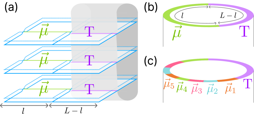
Figure 2: (a) Path-integral representation of $Z_{n}(A)$. A boundary condition $\vec{\mu}$ is imposed on the $n$-sheeted Riemann surface in $0\,{\leq}\,x\,{\leq}\,l$, and branch points are located at $x\,{=}\,l,L$. (b) Cylinder geometry under the periodic boundary conditions with the uniform measurement outcomes $\vec{\mu}$. (c) In general, there exist multiple domains $\vec{\mu}_{i\in\{1,2,\ldots\}}$ where the outcomes are uniform.

For the sake of simplicity, we shall first consider $S_{A}^{\vec{\mu}}$, the swapped EE in the case of the uniform outcomes. With proper normalization, the path integral of the corresponding replicated CFT reads (see Fig. 2 (a))

$$\Tr[(\rho^{\vec{\mu}}_{A})^{n}]=\frac{Z_{n}(A)}{Z^{n}}\equiv\frac{\int_{\vec{\mu},\mathrm{T}}\!\mathcal{D}\vec{\bm{\phi}}\;e^{-\sum_{k=1}^{n}\mathcal{S}[\bm{\phi}^{(k)}]}}{\quantity(\int_{\vec{\mu}}\mathcal{D}\vec{\bm{\phi}}\;e^{-\mathcal{S}[\bm{\phi}]})^{n}}.$$ (4)

Here, $\mathcal{D}\vec{\bm{\phi}}=\mathcal{D}\bm{\phi}^{(1)}\cdots\mathcal{D}\bm{\phi}^{(n)}$ is the measure of the path integral for replicated fields $\bm{\phi}^{(k)}$ ($k\,{\in}\,\{1,2,{\ldots},n\}$). The boundary conditions are denoted by $\vec{\mu}$ and $\mathrm{T}$, which correspond to the following conditions on the two-dimensional sheet $(x,\tau)\in[0,L]{\times}[0,\beta]$:

$$\vec{\mu} :\;\bm{\phi}^{(k)}(x,0)=\bm{\phi}^{(k)}(x,\beta)=\bm{\phi}^{\vec{\mu}}(x)\quad(0\leq x\leq l),$$ (5)

$$\mathrm{T} :\left\{\begin{aligned} \phi^{(k)}_{1}(x,\beta)&=\phi^{(k)}_{1}(x,0)&&(l<x\leq L)\\ \phi^{(k)}_{2}(x,\beta)&=\phi^{(k+1)}_{2}(x,0)&&(l<x\leq L)\end{aligned}\right..$$ (6)

Here, $\bm{\phi}^{\vec{\mu}}(x)$ is the field configuration that corresponds to the low-energy description of the product of Bell states $\bigotimes_{j=j^{\prime}=1}^{l}\!\ket*{\mathrm{Bell}^{\mu}_{jj^{\prime}}}$.

In general, a boundary of a CFT in the infrared limit is described by a conformally invariant boundary condition which is determined by the boundary condition imposed at the microscopic scale. When two neighboring segments of the boundary are subject to conformally invariant boundary conditions, we can interpret it as an insertion of BCCO at the point separating the two segments. In the present case, $Z_{n}(A)$ and $Z$ have the BCCOs from $\vec{\mu}$ to $\mathrm{T}$ and $\vec{\mu}$ to $\mathrm{F}$ at $x=l$, respectively. Here, $\mathrm{F}$ represents the free boundary conditions. Thus, if the boundary condition $\vec{\mu}$ is conformally invariant, the partition functions can be expressed as two-point correlation functions of the BCCOs,

$$Z_{n}(A)\!=\!\expectationvalue{\mathcal{B}_{\mathrm{T}|\vec{\mu}}(l)\mathcal{B}_{\vec{\mu}|\mathrm{T}}(0)}_{n},\;\;Z\!=\!\expectationvalue{\mathcal{B}_{\mathrm{F}|\vec{\mu}}(l)\mathcal{B}_{\vec{\mu}|\mathrm{F}}(0)}_{1},$$ (7)

where $\expectationvalue*{\cdots}_{n}$ denotes an expectation value with respect to the $n$ replicated fields, and $\mathcal{B}_{b|a}(x)$ is the BCCO that changes the boundary condition from $a$ to $b$ at point $x$.

Since two-point correlation functions in CFT can be determined from the scaling dimensions of the operators, we have $\expectationvalue*{\mathcal{B}_{\mathrm{T}|\vec{\mu}}(l)\mathcal{B}_{\vec{\mu}|\mathrm{T}}(0)}_{n}\,{=}\,l^{-2\Delta_{\mathrm{T}|\vec{\mu}}}$ and $\expectationvalue*{\mathcal{B}_{\mathrm{F}|\vec{\mu}}(l)\mathcal{B}_{\vec{\mu}|\mathrm{F}}(0)}_{1}\,{=}\,l^{-2\Delta_{\mathrm{F}|\vec{\mu}}}$, where $\Delta_{b|a}$ denotes the scaling dimension of $\mathcal{B}_{b|a}(x)$. More precisely, in the cylinder geometry considered here, the interval $l$ should be replaced by the chord length $l_{c}\,{=}\,(L/\pi)\sin(\pi l/L)$. Consequently, the swapped entanglement $S^{\vec{\mu}}_{A}$ obeys the logarithmic scaling

$$S^{\vec{\mu}}_{A}=-\lim_{n\to 1}\frac{\partial}{\partial n}\frac{Z_{n}(A)}{Z^{n}}\sim c_{\vec{\mu}}\ln\quantity[\frac{L}{\pi}\sin(\frac{\pi l}{L})].$$ (8)

Here, we introduce the universal coefficient,

$$c_{\vec{\mu}}=\lim_{n\to 1}\frac{2(\Delta_{\mathrm{T}|\vec{\mu}}-n\Delta_{\mathrm{F}|\vec{\mu}})}{n-1},$$ (9)

which is determined by the scaling dimensions of the BCCOs.

The above argument can be extended to the case of a general measurement outcome $\vec{m}$. Let $x_{i}$ denote the boundary condition changing points for $\vec{m}$. Suppose that the domains between those points, where the outcomes are the same, extend over the regions longer than the lattice constant so that the continuum description remains valid. The path-integral representation of $S^{\vec{m}}_{A}$ can then be obtained as a multipoint correlation function of the BCCOs as follows (Fig. 2 (c)):

$$\Tr[(\rho^{\vec{m}}_{A})^{n}]=\frac{\expectationvalue*{\prod_{i}\mathcal{B}_{b_{i+1}|b_{i}}(x_{i})}_{n}}{\expectationvalue*{\prod_{i}\mathcal{B}_{a_{i+1}|a_{i}}(x_{i})}_{1}^{n}}.$$ (10)

Here, $b_{i}$ is either the sewing condition ($\mathrm{T}$) or a boundary condition induced by any of the Bell bases ($\vec{\mu}$), and $a_{i}$ is the same as in $b_{i}$ except that $\mathrm{T}$ should be replaced by $\mathrm{F}$.

We may also express the averaged swapped EE $\overline{S}_{A}$ by employing the replica trick. To see this, we introduce the unnormalized density matrices $\tilde{\rho}^{\vec{m}}{=}\,p_{\vec{m}}\outerproduct*{\Psi^{\vec{m}}}{\Psi^{\vec{m}}}$ and $\tilde{\rho}^{\vec{m}}_{A}{=}\,p_{\vec{m}}\rho^{\vec{m}}_{A}$. The averaged one then reads

$$\overline{S}_{A}=\lim_{\begin{subarray}{c}n\to 1\\ s\to 0\end{subarray}}\sum_{\vec{m}}\frac{\Tr[\tilde{\rho}^{\vec{m}}]\Tr[(\tilde{\rho}^{\vec{m}}_{A})^{n}]^{s}-\Tr[\tilde{\rho}^{\vec{m}}]^{ns+1}}{s(1-n)}.$$ (11)

This expression corresponds to a path integral of $ns{+}1$ replicas with certain boundary interactions. When the boundary conditions are conformally invariant, the averaged swapped EE $\overline{S}_{A}$ also obeys the universal logarithmic scaling as demonstrated below.

Entanglement swapping in critical XXZ chains.— As a concrete example, we consider the entanglement swapping in the two copies of the spin-$\frac{1}{2}$ critical XXZ chain,

$$H=\sum_{j=1}^{L}(\sigma_{j}^{x}\sigma_{j+1}^{x}+\sigma_{j}^{y}\sigma_{j+1}^{y}+\Delta\sigma_{j}^{z}\sigma_{j+1}^{z}),\;\;\Delta\in(-1,1],$$ (12)

whose effective field theory is given by a $c\,{=}\,1$ CFT with the TLL parameter $K\,{=}\,\pi/(2\pi\,{-}\,2\cos^{-1}\Delta)$ [105]. We recall that the TLL is described by a boson field $\phi$ and its dual $\theta$, which are compactified as $\phi\,{\sim}\,\phi\,{+}\,\pi n,\theta\,{\sim}\,\theta\,{+}\,2\pi m\;(n,m\,{\in}\,\mathbb{Z})$. These fields can be related to the $j$-th qubit $\sigma_{j}^{\alpha}\;(\alpha\,{=}\,x,y,z)$ by

$$\sigma_{j}^{z} \simeq\frac{2}{\pi}\partial_{x}\phi+\frac{(-1)^{j}}{\pi\gamma}\cos(2\phi),$$ (13)

$$\sigma_{j}^{x}\pm i\sigma_{j}^{y} \simeq\frac{e^{\pm i\theta}}{\sqrt{\pi\gamma}}\quantity[(-1)^{j}+\cos(2\phi)],$$ (14)

where $\gamma$ is a nonuniversal constant of order unity. The bosonic fields corresponding to each of the two chains are denoted by $\phi,\phi^{\prime}$, respectively, and we write their duals as $\theta,\theta^{\prime}$.

To determine the universal coefficient $c_{\vec{\mu}}$ in Eq. (8), we first need to identify the conformal boundary conditions induced by the measurement operator $P^{\vec{\mu}}$. Using the path-integral representation and the bosonization relation, we can represent the Bell-state measurement as a boundary perturbation $P^{\vec{\mu}}\,{=}\,e^{-\delta\mathcal{S}}$ with the boundary action $\delta\mathcal{S}$ being given by

$$\delta\mathcal{S}=-\lim_{g\to\infty}g\int_{0}^{l}\!dx\int_{0}^{\beta}\!d\tau\delta(\tau)\Bigl{[}\;(-1)^{b_{2}}\cos\theta_{b_{1}}\\ +(-1)^{b_{1}}\frac{\cos(2\phi_{+})+\cos(2\phi_{-})}{2\pi\gamma}\Bigr{]},$$ (15)

where $\phi_{\pm}\,{=}\,\phi\pm\phi^{\prime}$, $\theta_{\pm}\,{=}\,\theta\pm\theta^{\prime}$, and $\theta_{b_{1}=0/1}$ represents $\theta_{+/-}$, respectively. The resulting boundary condition is the configuration that minimizes $\delta\mathcal{S}$. Consequently, there are four possible boundary conditions depending on the measurement outcomes, where the boson fields are locked at the boundary such that $(\phi_{-},\theta_{+}){=}(0,0)$, $(\phi_{-},\theta_{+}){=}(0,\pi)$, $(\phi_{+},\theta_{-}){=}(\pi/2,0)$, and $(\phi_{+},\theta_{-}){=}(\pi/2,\pi)$ for $\mu\,{=}\,00,01,10,11$, respectively. These mixed Dirichlet-Neumann conditions are known to be conformally invariant [91]. We note that the configuration corresponding to $\mu{=}10$ ($\mu{=}11$) has been also known to represent the rung singlet^∗ (rung singlet) phase in the spin-$\frac{1}{2}$ XXZ ladder [106, 107, 108, 109].

We next derive the scaling dimensions of the BCCOs $\mathcal{B}_{\mathrm{T}|\vec{\mu}}$ and $\mathcal{B}_{\mathrm{F}|\vec{\mu}}$. For this purpose, we note that the scaling dimension of $\mathcal{B}_{b|a}$ can be related to the ground-state energy of the corresponding CFT on a strip geometry where boundary conditions $a$ and $b$ are imposed on each side [110] (see Supplemental Material (SM) [111] for details). This correspondence allows us to obtain

$$\Delta_{\mathrm{T}|\vec{\mu}}=\frac{n}{6}-\frac{1}{24n},\;\Delta_{\mathrm{F}|\vec{\mu}}=\frac{1}{8}.$$ (16)

From Eq. (9), we thus have $c_{\vec{\mu}}\,{=}\,1/6$ as the universal coefficient in the entanglement swapping in TLLs.

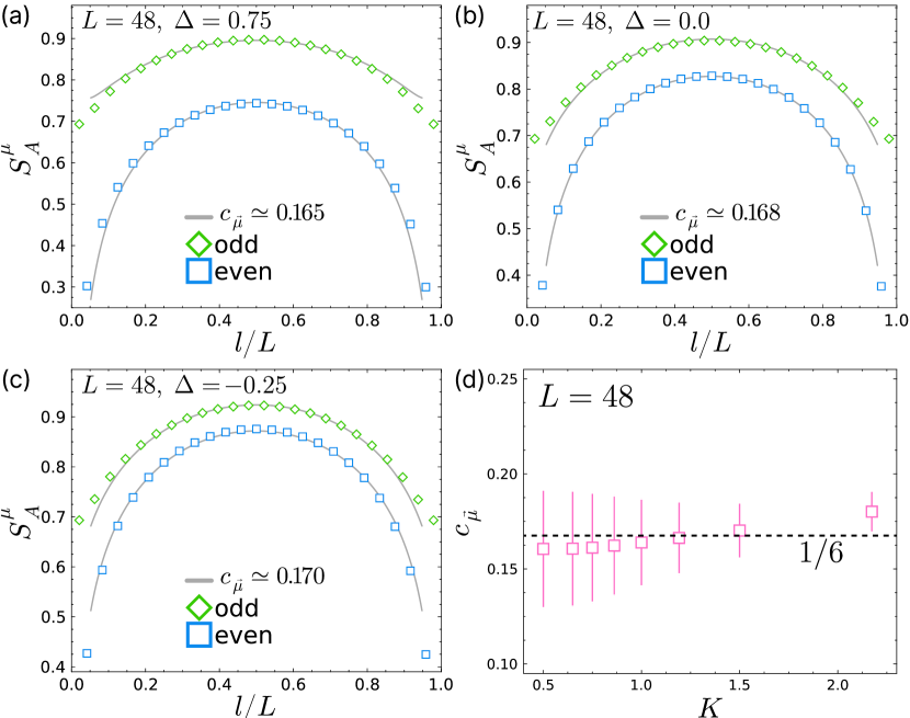
Figure 3: (a,b,c) Numerical results of $S^{\vec{\mu}}_{A}$ at different $\Delta$ plotted as a function of $l/L$. Markers are changed for $l$ even and odd. The black curves are obtained by fitting the results to Eq. (17). The fitting parameters at $\Delta\,{=}\,0.75$, $0.0$, and $-0.25$ are $(c_{\vec{\mu}},c_{1},c_{2})=(0.165,-0.44,0.05)$, $(0.168,-0.24,0.12)$, and $(0.170,-0.15,0.13)$, respectively. (d) The universal coefficient $c_{\vec{\mu}}$ plotted against $K$. Error bars indicate variations when the region used for the fitting is varied.

To numerically test the above results, we perform matrix product states (MPS) calculations of the entanglement swapping in the XXZ chains. Since the swapped entanglement $S_{A}^{\vec{\mu}}$ takes the same value for all four Bell bases $\vec{\mu}$ in the present case, it suffices to focus on a particular $\vec{\mu}$ here. This is because the Bell bases relate to each other by a qubit-wise unitary operator, and the initial state is invariant under this unitary operation due to the global $\mathbb{Z}_{2}$ symmetry. Figure 3 (a,b,c) verifies the predicted logarithmic scaling of $S^{\vec{\mu}}_{A}$ as a function of the number of measured qubits $l$. Additionally, we observe an even-odd oscillation depending on $l$. This parity effect is analogous to what has been found in the entanglement entropy of an XXZ chain with open boundary conditions [112, 113, 114], indicating that the projective measurements effectively create open ends in the chains. Following Refs. [112, 113, 114], we consider the fitting function that includes this oscillation term,

$$S^{\vec{\mu}}_{A}\!=\!c_{\vec{\mu}}\ln\quantity[\frac{L}{\pi}\sin(\frac{\pi l}{L})]\!+\!c_{1}(c_{2}+(-1)^{l})\quantity[\frac{L}{\pi}\sin(\frac{\pi l}{L})]^{-K},$$ (17)

where $c_{1},c_{2}$ are nonuniversal constants whose values are provided in the caption of Fig. 3. Figure 3 (d) shows the estimated value of the coefficient $c_{\vec{\mu}}$ at different $K$, which confirms the predicted universal value $c_{\vec{\mu}}\,{=}\,1/6$ within the error bars. We note that the data points close to the edges ($l\,{\sim}\,0,L$) are not included in the fitting since they substantially deviate from the logarithmic behavior due to the short-distance effect. The error bars in Fig. 3 (d) are mainly due to the fact that the estimated values of $c_{\vec{\mu}}$ exhibit relatively large fluctuations depending on whether the number of those excluded data points were even or odd.

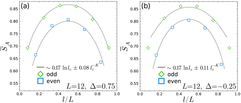
Figure 4: (a,b) Numerical results of the averaged swapped entanglement $\overline{S}_{A}$ at (a) $\Delta{=}0.75$ and (b) $\Delta{=}{-}0.25$. Fitting curves are shown in the legend as a function of $l_{c}{=}(L/\pi)\sin(\pi l/L)$. Statistical errors are small enough compared to the size of the markers.

We next numerically evaluate the averaged swapped entanglement $\overline{S}_{A}$, where the ensemble average is taken over all the possible measurement outcomes (see Eq. (3)). Interestingly, as shown in Fig. 4, we find that $\overline{S}_{A}$ again exhibits the logarithmic scaling and the parity effect, which are akin to what we find in the uniform outcome cases above. In particular, the estimated value of the coefficient in the logarithmic term ($0.17$) is close to that of the uniform case $c_{\vec{\mu}}\,{=}\,1/6$. These results suggest that the measurement-induced boundary interactions in the CFT of $ns{+}1$ replicas in Eq. (11) lead to certain conformal boundary conditions, and the scaling dimension of the corresponding BCCO should be the same as in the uniform case (see SM [111] for further discussions).

Experimental accessibility.— Our consideration should be relevant to current experiments. The key requirements for the entanglement swapping proposed in this paper are the preparation of the critical states, the Bell-state measurements, and the evaluation of the EE. All these techniques are within reach of current programmable quantum platforms [115, 116], such as Rydberg atom arrays [94, 95]. We note that our setup does not include mid-circuit measurements as in hybrid quantum circuits [97], and the post-measurement state is pure. Also, the signature of the universality in the swapped entanglement is appreciable even in a small system with, e.g., ten qubits. Thus, an experiment with brute-force postselections and/or quantum state tomography might be feasible. To circumvent the exponential overhead for a larger number of qubits, it might be useful to employ recent suggestions of mutually unbiased bases quantum state tomography [117], MPS tomography [118, 119], machine-learning approaches [120, 121], classical shadows technique [122, 123], and classical simulation-assisted schemes [124, 125].

Conclusion.— We have shown that the swapped entanglement in critical spin chains can exhibit the universal logarithmic behavior. We have provided a boundary CFT prescription for calculating the universal coefficient when the Bell-state measurement outcomes are uniform (cf. Eqs. (8) and (9)). The field-theoretical results have been confirmed in the case of critical XXZ chains through numerical calculations (cf. Fig. 3). A similar universal behavior has been observed numerically when the ensemble average is taken over all the measurement outcomes (cf. Fig. 4).

There are several intriguing directions for future studies. First, it merits further study to understand entanglement swapping of critical states in a different universality class, such as the Ising criticality. Our initial analysis suggests that the universal logarithmic behavior can also be found in the Ising class, while its full understanding requires a further investigation (see SM [111] and Refs. [126, 127]).

Secondly, it is of practical importance to identify what would be the most efficient entanglement swapping protocol. One can, for instance, optimize a choice of the type/number of the initial chains and/or the measurement basis to maximize the amount of the swapped entanglement. Our findings suggest that, among all the possible measurements that lead to the conformal boundary conditions, the one with the highest scaling dimension should be the optimal choice.

Lastly, it would be worthwhile to consider a possible extension of our boundary CFT analysis to the problem of quantum state learning [128, 129, 130, 131]. While there have been significant advances in our understanding of the effects of measurement backaction on critical states, their implications from a perspective of the learnability of quantum states is largely unexplored. Our approach allows for a quantitatively accurate characterization of long-distance entanglement properties in a post-measurement state, which might be useful also in this context. We hope that our study stimulates further studies in these directions.

Supplemental Material for “Entanglement swapping in critical spin chains”

SI Derivation of the scaling dimensions of the BCCOs

In this section, we derive the scaling dimensions of the BCCOs in the case of the entanglement swapping in the XXZ chains (Eq. (16) in the main text). To this end, we first review the procedure to calculate the scaling dimension of a BCCO. We then derive the logarithmic scaling of the entanglement entropy of a CFT from the viewpoint of the boundary CFT. Finally, we extend this method to the present case to determine the universal coefficient $c_{\vec{\mu}}$ in the main text.

SI.1 The scaling dimension of a BCCO

We first review the procedure to calculate the scaling dimension of a BCCO [110]. Consider a BCCO $\mathcal{B}_{b|a}(x)$ which changes the boundary condition from $a$ to $b$ on the upper half-plane ($\tau\geq 0$ with coordinates $z=x+i\tau$). If the boundary condition $b$ is imposed on the interval $[x_{1},x_{2}]$, the partition function of this theory is calculated from the two-point correlation function of the BCCOs as:

$$\expectationvalue*{\mathcal{B}_{b|a}(x_{1})\mathcal{B}_{a|b}(x_{2})}=\frac{1}{(x_{1}-x_{2})^{2\Delta_{b|a}}}.$$ (S1)

Under a conformal map $z=de^{\pi w/d}$ that maps the upper half-plane to an infinite strip with finite width $d$, the two-point correlation function (Eq. (S1)) transforms as:

$$\expectationvalue*{\mathcal{B}_{b|a}(u_{1})\mathcal{B}_{a|b}(u_{2})} =\quantity(\frac{dw}{dz})_{z=x_{1}}^{-\Delta_{b|a}}\quantity(\frac{dw}{dz})_{z=x_{2}}^{-\Delta_{b|a}}\frac{1}{(x_{1}-x_{2})^{2\Delta_{b|a}}}$$

$$=\quantity[\frac{2d}{\pi}\sinh\frac{\pi}{2d}(u_{1}-u_{2})]^{-2\Delta_{b|a}}$$

$$\to\quantity(\frac{\pi}{d})^{2\Delta_{b|a}}\exp(-\frac{\pi\Delta_{b|a}}{d}(u_{1}-u_{2}))\quad(u_{1}-u_{2}\to\infty).$$ (S2)

Here, $x_{1}=de^{\pi u_{1}/d}$ and $x_{2}=de^{\pi u_{2}/d}$. If we consider the quantization in such a way that the horizontal axis in the strip corresponds to the imaginary time (cf. Fig. S1), the two-point correlation function can be also calculated as follows:

$$\expectationvalue*{\mathcal{B}_{b|a}(u_{1})\mathcal{B}_{a|b}(u_{2})}=\expectationvalue*{\mathcal{B}_{b|a}(0)\mathcal{B}_{a|b}(\Delta u)} =\bra*{aa;0}\mathcal{B}_{b|a}(0)e^{-H_{ab}\Delta u}\mathcal{B}_{a|b}(0)e^{H_{aa}\Delta u}\ket*{aa;0}$$

$$=\sum_{n}\absolutevalue*{\bra*{aa;0}\mathcal{B}_{b|a}(0)\ket*{ab;n}}^{2}e^{-[E_{ab}^{n}(d)-E_{aa}^{0}(d)]\Delta u}$$

$$\to\absolutevalue*{\bra*{aa;0}\mathcal{B}_{b|a}(0)\ket*{ab;0}}^{2}e^{-[E_{ab}^{0}(d)-E_{aa}^{0}(d)]\Delta u}\quad(\Delta u=u_{1}-u_{2}\to\infty).$$ (S3)

Here, $H_{ab}$ ($H_{aa}$) is the Hamiltonian of the segment of length $d$ with boundary conditions $a$ and $b$ ($a$ and $a$) on each side, $E_{ab}^{n}(d)$ ($E_{aa}^{n}(d)$) is the $n$-th energy eigenvalue of this Hamiltonian, and $\ket*{ab;n}$ ($\ket*{aa;n}$) is the corresponding eigenstate (see Fig. S1). Comparing the two expressions (Eq. (SI.1) and Eq. (SI.1)) for the two-point correlation function, we obtain the following relation:

$$\frac{\pi\Delta_{b|a}}{d}=E_{ab}^{0}(d)-E_{aa}^{0}(d).$$ (S4)

Thus, we can calculate the scaling dimension $\Delta_{b|a}$ of a BCCO $\mathcal{B}_{b|a}$ from the ground-state energy of the CFT on an infinite strip of width $d$, where the boundary conditions $a$ and $b$ are imposed on each side. Determining the ground-state energy for a general geometry is not an easy task. However, if the CFT is on a cylinder (as will be discussed later), the ground-state energy is known to be the Casimir energy:

$$E=-\frac{\pi}{6}\frac{c}{L}.$$ (S5)

Here, $L$ is the circumference of the cylinder, and $c$ is the central charge.

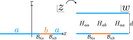
Figure S1: The upper half-plane maps to an infinite strip under a conformal map $z=de^{\pi w/d}$. Quantization along the strip gives two different Hamiltonians $H_{ab}$ and $H_{aa}$ depending on the boundary conditions.

SI.2 Entanglement entropy of a finite interval in a CFT

Here, we derive the well-known result [100, 101] on the entanglement entropy of a finite interval in a CFT, in terms of BCCOs. Although our derivation is essentially identical to the original ones, it is clarifying and also allows a systematic generalization to a variety of problems as we will discuss next in subsection SI.3. Let us assume that a CFT is described in terms of a field $\phi$. In the path-integral representation, the matrix element of the reduced density matrix of a finite interval $I$ reads:

$$\rho_{I}(\phi_{1}(x),\phi_{2}(x))\propto\int\mathcal{D}\vec{\phi}\;e^{-\mathcal{S}[\vec{\phi}]},$$ (S6)

where $\mathcal{S}[\vec{\phi}]$ is the action of the doubled CFT, which is described in terms of the two-component field $\vec{\phi}=(\phi_{1},\phi_{2})$ defined on the upper half-plane $\tau\geq 0$. In the bulk $\tau>0$, the action is just the sum of the actions for $\phi_{1}$ and $\phi_{2}$, i.e., the two fields are only coupled at the boundary $\tau=0$. Outside the interval $I$, the boundary condition $\phi_{1}=\phi_{2}$ is imposed, which corresponds to taking the partial trace over $\overline{I}$. For normalization of $\rho_{I}$, we need to divide the right hand side of Eq. (S6) with the partition function:

$$Z=\int\mathcal{D}\vec{\phi}\;e^{-\mathcal{S}[\vec{\phi}]}.$$ (S7)

Here, the boundary condition $\phi_{1}=\phi_{2}$ is imposed on the entire boundary. Since this does not contain any change to the boundary, it only gives a nonuniversal constant independent of the interval length.

The entanglement entropy $S_{I}=-\Tr[\rho_{I}\ln\rho_{I}]$ can be obtained from the $n{\to}1$ limit of $-\partial_{n}\Tr[(\rho_{I})^{n}]$. To calculate $\Tr[(\rho_{I})^{n}]$, we use the replica trick, i.e., we consider the partition function of $2n$ replicas as follows:

$$\Tr[(\rho_{I})^{n}]=\frac{Z_{n}(I)}{Z^{n}}.$$ (S8)

Here $Z_{n}(I)$ is the path integral of $2n$ replicas $(\phi_{1},\phi_{2},\ldots,\phi_{2n})$ with the boundary conditions

$$A :\quad\phi_{2j-1}=\phi_{2j}\;(x\notin I),$$ (S9)

$$B :\quad\phi_{2j}=\phi_{2j+1}\;(x\in I).$$ (S10)

Here, $\phi_{2n+1}\equiv\phi_{1}$. The partition function $Z_{n}(I)$ can be interpreted as a two-point function of BCCOs $\mathcal{B}_{A|B}$ inserted at the ends of $I$ (see Fig. S2).

As explained in the previous subsection, the scaling dimension of the BCCO $\mathcal{B}_{A|B}$ is related to the ground-state energy $E_{AB}^{0}(d)$ of the CFT on an infinite strip of width $d$, where the boundary conditions $A$ and $B$ are imposed on each side (see Fig. S2(a)). Suppose that we impose the boundary condition $A$ on the left and $B$ on the right. Let us start from $\phi_{1}$ and follow it to the left. At the left boundary, this is connected to $\phi_{2}$ as $\phi_{1}=\phi_{2}$. Now following $\phi_{2}$ to the right, it is connected to $\phi_{3}$. Repeating this process $2n$ times, we return to $\phi_{1}$. Namely, the replicas form a single loop. Thus, the ground-state energy $E_{AB}^{0}(d)$ is identical to the ground-state energy of the original (single-component) CFT on a cylinder of circumference $2dn$:

$$E_{AB}^{0}(d)=-\frac{\pi}{6}\frac{c}{2dn}=-\frac{\pi c}{12dn}.$$ (S11)

This is to be compared with the ground-state energy $E_{AA}^{0}(d)$ of the $2n$-component CFT on the same strip geometry with the boundary condition $A$ on both sides. Each component of the field is coupled to its partner ($\phi_{2j-1}$ and $\phi_{2j}$) at both sides. Now, the replicas form $n$ loops by paring up with partners. Thus, the ground-state energy $E_{AA}^{0}(d)$ is given by $n$ times the ground-state energy of the original CFT on a cylinder of circumference $2d$:

$$E_{AA}^{0}(d)=-\frac{\pi}{6}\frac{c}{2d}\times n=-\frac{\pi nc}{12d}.$$ (S12)

The scaling dimension $\Delta_{A|B}$ of the BCCO $\mathcal{B}_{A|B}$ is now calculated from Eq. (S4) as

$$\frac{\pi\Delta_{AB}}{d}=E_{AB}^{0}(d)-E_{AA}^{0}(d)=\frac{\pi c}{12d}\quantity(n-\frac{1}{n}),$$ (S13)

which implies

$$\Delta_{AB}=\frac{1}{12}\quantity(n-\frac{1}{n}).$$ (S14)

Using the BCCOs, the partition function $Z_{n}(I)$ reads

$$Z_{n}(I)=\expectationvalue*{\mathcal{B}_{AB}(l)\mathcal{B}_{BA}(0)}=l^{-2\Delta_{AB}}=l^{-\frac{1}{6}\quantity(n-\frac{1}{n})},$$ (S15)

leading to the well-known formula for general CFTs:

$$S_{I}=\lim_{n\to 1}-\frac{\partial}{\partial n}\ln\frac{Z_{n}(I)}{Z^{n}}=\frac{c}{3}\ln l+\text{const.}$$ (S16)

Note that since $Z$ is independent of the interval length $l$, the denominator only gives a nonuniversal constant to the entanglement entropy $S_{I}$. Although the normalization is relatively simple in this problem, it will be more nontrivial and interesting in our setup for the entanglement swapping.

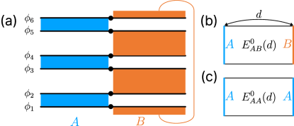
Figure S2: (a) The two boundary conditions $A$ and $B$. $A$ corresponds to taking the partial trace and $B$ is the sewing condition. (b) The strip of width $d$ with the boundary conditions $A$ and $B$ on each side. (c) The same strip geometry with the boundary condition $A$ on both sides.

SI.3 The swapped entanglement between two TLLs

We now extend the above discussion to the setup of the entanglement swapping in the two TLLs and derive the scaling dimensions of the BCCOs ($\mathcal{B}_{\mathrm{T}|\vec{\mu}}$ and $\mathcal{B}_{\mathrm{F}|\vec{\mu}}$ in the main text), which give the universal coefficient in the swapped entanglement. Consider two decoupled TLLs of length $L$. We measure $l$ qubits in the Bell basis, and the unmeasured intervals of length $l_{I}=L-l$ get entangled. If the measurement outcomes are uniform in one of the Bell bases, say $\ket*{\mathrm{Bell}^{00}}=(\ket*{00}+\ket*{11})/\sqrt{2}$, the following boundary condition is imposed on the measured interval:

$$\phi_{-} \equiv\phi_{1}-\phi_{2}=0,$$ (S17)

$$\theta_{+} \equiv\theta_{1}+\theta_{2}=0.$$ (S18)

Here, $\phi_{1}$ and $\phi_{2}$ are the boson fields describing the TLLs, and $\theta_{1}$ and $\theta_{2}$ are their duals.

In the doubled-Hilbert space formalism above, the density matrix for the present system is obtained by the partition function of a four-component free boson field theory. On the measured interval, the boundary conditions are

$$\phi_{1}-\phi_{2}=\phi_{3}-\phi_{4} =0,$$ (S19)

$$\theta_{1}+\theta_{2}=\theta_{3}+\theta_{4} =0.$$ (S20)

Here we adopt the convention that $\phi_{3,4}$ are the counterparts of $\phi_{1,2}$ in the doubled-Hilbert space. We note that the Dirichlet condition on $\theta_{+}$ is equivalent to the Neumann condition on $\phi_{+}$. Since the first condition in Eq. (S19) implies $\phi_{1}=\phi_{2}$ on the boundary, the Neumann condition on $\phi_{+}=\phi_{1}+\phi_{2}$ is the same as the Neumann condition on $\phi_{1}\;(=\phi_{2})$. Thus, we do not need to consider the conditions for $\theta$ explicitly when we formulate the problem in terms of $\phi$ fields. Let us denote this boundary condition in Eq. (S19) by $\vec{\mu}$.

To obtain the $n$-th power of the reduced density matrix $\Tr[(\rho^{\vec{\mu}}_{I})^{n}]$, we need the partition function of the replicas $Z_{n}(I)$ and the original partition function $Z$ for normalization. As mentioned above, we emphasize that the original partition function $Z$ also depends on the interval length $l_{I}$ nontrivially in the present case. We can calculate $Z$ by taking the trace over the unmeasured interval $I$, which is described by the following boundary conditions:

$$\phi_{1}-\phi_{3}=\phi_{2}-\phi_{4}=0.$$ (S21)

Let us denote this boundary condition by $\mathrm{F}$. Accordingly, $Z$ is given by a two-point function of the BCCO $\mathcal{B}_{\mathrm{F}|\vec{\mu}}$ inserted at the ends of the interval $I$. The scaling dimension of $\mathcal{B}_{\mathrm{F}|\vec{\mu}}$ is determined from the ground-state energy $E_{\mathrm{F}\vec{\mu}}^{0}(d)$ of the four-component boson field theory on a strip of width $d$ with boundary conditions $\mathrm{F}$ and $\vec{\mu}$ on each side (see Fig. S3). We see that the four boson fields form a closed loop of length $4d$. Thus

$$E_{\mathrm{F}\vec{\mu}}^{0}(d)=-\frac{\pi}{6}\frac{1}{4d}=-\frac{\pi}{24d}.$$ (S22)

When the boundary conditions are $\mathrm{F}$ on both sides, the four fields form two loops with their partners. Thus, the ground-state energy $E_{\mathrm{F}\mathrm{F}}^{0}(d)$ is two times the ground-state energy of the $c=1$ free boson CFT on a cylinder of circumference $2d$, namely,

$$E_{\mathrm{F}\mathrm{F}}^{0}(d)=-\frac{\pi}{6}\frac{1}{2d}\times 2=-\frac{\pi}{6d}.$$ (S23)

The scaling dimension $\Delta_{\mathrm{F}|\vec{\mu}}$ is then obtained from the following relation:

$$\frac{\pi\Delta_{\mathrm{F}|\vec{\mu}}}{d}=E_{\mathrm{F}\vec{\mu}}^{0}(d)-E_{\mathrm{F}\mathrm{F}}^{0}(d)=\frac{\pi}{8d},$$ (S24)

which implies $\Delta_{\mathrm{F}|\vec{\mu}}=1/8$. Thus, the original partition function $Z$ has a nontrivial dependence on the interval length as follows:

$$Z=\expectationvalue*{\mathcal{B}_{\mathrm{F}|\vec{\mu}}(l)\mathcal{B}_{\vec{\mu}|\mathrm{F}}(0)}_{1}\propto l^{-1/4}.$$ (S25)

In a system with finite size $L$ under the periodic boundary conditions, $l$ should be replaced by the chord length $l_{c}=(L/\pi)\sin(\pi l/L)$.

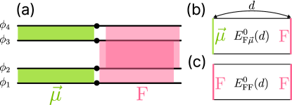
Figure S3: (a) Boundary conditions $\mathrm{F}$ and $\vec{\mu}$. $\mathrm{F}$ corresponds to taking the trace and $\vec{\mu}$ is the boundary condition induced by the measurements. (b) The strip of width $d$ with the boundary conditions $\mathrm{F}$ and $\vec{\mu}$ on each side. (c) The same strip geometry with the boundary condition $\mathrm{F}$ on both sides.

However, in the above analysis, the nonuniversal boundary energy density was not taken into account. The boundary condition $\mathrm{F}$ corresponds to just folding the bulk, so there should be no boundary energy. On the other hand, the boundary condition $\vec{\mu}$ can have a nonvanishing nonuniversal boundary energy $\epsilon_{\vec{\mu}}$ per unit length. Including this effect, we have

$$Z\sim e^{-\epsilon_{\vec{\mu}}l}\quantity(\frac{L}{\pi}\sin\frac{\pi l}{L})^{-1/4}.$$ (S26)

Note that we cannot replace $l$ by $l_{c}$ in the exponential factor. The original partition function calculated here is actually the Born probability $p_{\vec{\mu}}=\|P^{\vec{\mu}}\ket*{\Psi_{0}}\!\otimes\!\ket*{\Psi_{0}}\|^{2}$ for obtaining the uniform measurement outcomes. The above relation has been confirmed by the numerical calculations as shown in Fig. S4.

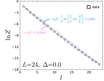
Figure S4: Numerical results of the $l$ dependence of the partition function $Z$, which corresponds to the Born probability of obtaining a uniform measurement outcome. The power-law correction to the exponential decay is crucial for the precise fitting. The fitting to Eq. (S26) leads to $\epsilon_{\vec{\mu}}=0.693(\approx\ln 2)$. This means that the probability of obtaining a uniform outcome is approximately $p_{\vec{\mu}}\approx 2^{-l}$.

We will now calculate $Z_{n}(I)$, which is the partition function of a $4n$-component free boson with certain boundary conditions. On the measured interval, the boundary conditions are

$$\phi_{4j-3}-\phi_{4j-2}=\phi_{4j-1}-\phi_{4j} =0,$$ (S27)

$$\theta_{4j-3}+\theta_{4j-2}=\theta_{4j-1}+\theta_{4j} =0,$$ (S28)

for $j\in\{1,2,\ldots,n\}$. This is just the boundary condition $\vec{\mu}$ imposed on each replica, and we use the same symbol $\vec{\mu}$ for this boundary condition. On the unmeasured interval, the boundary conditions are

$$\phi_{4j-2}=\phi_{4j},\;\phi_{4j-1}=\phi_{4j+1},$$ (S29)

for $j\in\{1,2,\ldots,n\}$ and $\phi_{4n+1}\equiv\phi_{1}$. This corresponds to taking the trace for the second TLL and sewing the replicas for the first TLL (see Fig. S5). Let us denote this boundary condition by $\mathrm{T}$.

Again, the scaling dimension of the BCCO $\mathcal{B}_{\mathrm{T}|\vec{\mu}}$ is obtained from the ground-state energy of the $4n$-component free boson field theory on an infinite strip of width $d$ with boundary conditions $\vec{\mu}$ and $\mathrm{T}$ on each side. We can see that $4n$ fields form a single loop. Thus, $E_{\vec{\mu}\mathrm{T}}^{0}(d)$ is given by the ground-state energy of the $c=1$ free boson CFT on a cylinder of circumference $4dn$:

$$E_{\vec{\mu}\mathrm{T}}^{0}(d)=-\frac{\pi}{6}\frac{1}{4dn}=-\frac{\pi}{24dn}.$$ (S30)

On the other hand, $E_{\vec{\mu}\vec{\mu}}^{0}(d)$ is given by $2n$ times the ground-state energy of the $c=1$ free boson CFT on a cylinder of circumference $2d$, since there are $2n$ loops formed by $2n$ pairs of boson fields $\phi_{2k-1}$ and $\phi_{2k}\;(k\in\{1,2,\ldots,2n\}$.

$$E_{\vec{\mu}\vec{\mu}}^{0}(d)=-\frac{\pi}{6}\frac{1}{2d}\times 2n=-\frac{\pi n}{6d}.$$ (S31)

The scaling dimension of the BCCO $\mathcal{B}_{\mathrm{T}|\vec{\mu}}$ is determined from

$$\frac{\pi\Delta_{\mathrm{T}|\vec{\mu}}}{d}=E_{\vec{\mu}\mathrm{T}}^{0}(d)-E_{\vec{\mu}\vec{\mu}}^{0}(d)=\frac{\pi n}{6d}-\frac{\pi}{24dn},$$ (S32)

and this implies $\Delta_{\mathrm{T}|\vec{\mu}}=n/6-1/24n$.

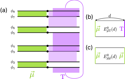
Figure S5: (a) Boundary conditions $\vec{\mu}$ and $\mathrm{T}$. $\vec{\mu}$ is the boundary condition induced by the measurements, and $\mathrm{T}$ corresponds to taking the trace on the second TLL, while sewing the replicas in the first TLL. (b) The strip of width $d$ with the boundary conditions $\vec{\mu}$ and $\mathrm{T}$ on each side. (c) The same strip geometry with the boundary condition $\vec{\mu}$ on both sides.

Altogether, we obtain

$$\Delta_{\mathrm{F}|\vec{\mu}} =\frac{1}{8},$$ (S33)

$$\Delta_{\mathrm{T}|\vec{\mu}} =\frac{n}{6}-\frac{1}{24n},$$ (S34)

$$\Tr[(\rho_{I}^{\vec{\mu}})^{n}]=\quad\frac{Z_{n}(I)}{Z^{n}} =\frac{\expectationvalue*{\mathcal{B}_{\mathrm{T}|\vec{\mu}}(l)\mathcal{B}_{\mathrm{T}|\vec{\mu}}(0)}_{n}}{\expectationvalue*{\mathcal{B}_{\mathrm{F}|\vec{\mu}}(l)\mathcal{B}_{\mathrm{F}|\vec{\mu}}(0)}_{1}^{n}}\sim l^{-2\Delta_{\mathrm{T}|\vec{\mu}}+2n\Delta_{\mathrm{F}|\vec{\mu}}}=l^{-\frac{1}{12}\quantity(n-\frac{1}{n})}.$$ (S35)

Therefore, the entanglement entropy of the swapped entanglement is

$$S_{I}=\frac{1}{6}\ln\quantity(\frac{L}{\pi}\sin\frac{\pi l}{L})+\text{const.}$$ (S36)

Additionally, the $n$-dependence of the Rényi entropy $S^{(n)}_{I}$ is apparent from this result:

$$S^{(n)}_{I}=\frac{1}{1-n}\ln\frac{Z_{n}(I)}{Z^{n}}=\frac{1}{12}\quantity(1+\frac{1}{n})\ln\quantity(\frac{L}{\pi}\sin\frac{\pi l}{L})+\text{const.}$$ (S37)

We confirmed this behavior by numerical calculations (see Fig. S6).

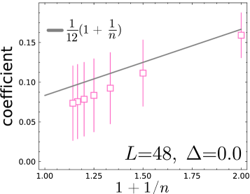
Figure S6: The $n$-dependence of the coefficient of the logarithmic scaling part of the Rényi entropy.

SII Details of numerical calculations

Our numerical calculations use matrix product states (MPS) to represent many-body wave functions. The measurement process is represented as a contraction of matrix product operators (MPOs) with MPS. The initial state $\ket*{\Psi_{0}}\!\otimes\!\ket*{\Psi_{0}}$ is prepared in $2L$-qubit MPS as shown in Fig. S7. This state is the ground state of the Hamiltonian $H\otimes H$, obtained by running the DMRG algorithm. Here, $H$ is the $L$-qubit Hamiltonian of the critical spin chain. We can use the same method for other models simply by changing the Hamiltonian.

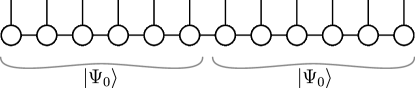
Figure S7: The initial state $\ket*{\Psi_{0}}\!\otimes\!\ket*{\Psi_{0}}$ represented as a $2L$-qubit MPS. This MPS is obtained by running the DMRG algorithm with the Hamiltonian $H\otimes H$.

Measurements are performed by expressing the projection operator $P^{b_{1}b_{2}}_{j,j^{\prime}}=\outerproduct*{\mathrm{Bell}^{b_{1}b_{2}}_{jj^{\prime}}}{\mathrm{Bell}^{b_{1}b_{2}}_{jj^{\prime}}}$ with an MPO. We measure the qubit pairs in the order $(L,L+1),(L-1,L+2),\ldots,(L-l+1,L+l)$, so that the subsystems $A$ and $A^{\prime}$ become $(1,2,\ldots,L-l)$ and $(L+l+1,\ldots,L)$, respectively. If we naively continue this procedure, the bond dimension between qubits $L$ and $L+1$ becomes exponentially large as $l$ increases, making the calculation very inefficient. This is because the entanglement between both sides is large due to the Bell states created by the measurements. To avoid this difficulty, we switch the site labels so that the center bond does not carry Bell states on both sides (see Fig. S8). Switching site labels in MPS can be done at an affordable cost with singular value decompositions (SVD).

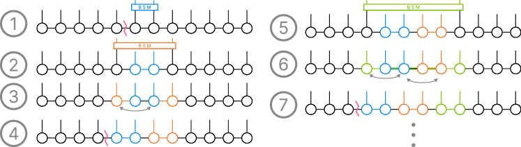
Figure S8: Steps to avoid the exponentially growing bond dimension in the center. After creating a Bell state with measurement, we switch site labels so that the Bell states do not overlap. The red zig-zag displays the bipartitioning point.

Finally, we calculate the entanglement entropy by bipartitioning the MPS into $A$ and the rest of the chain. Although this bipartition includes regions $\overline{A},\overline{A^{\prime}}$, it gives the same EE as $S^{\vec{m}}_{A}$. In this way, we can efficiently calculate the swapped entanglement while dealing with two spin chains.

SIII Boundary conditions for the averaged swapped entanglement

As discussed in the main text, the averaged swapped entanglement $\overline{S}_{A}$ can be calculated by the replica trick, where the measurement-induced boundary interactions are expected to lead to certain conformal boundary conditions. Here, we discuss the possible boundary condition realized in this replicated theory by focusing on the case of the XXZ critical chains.

To this end, we recall that the averaged swapped entanglement is expressed as follows:

$$\overline{S}_{A} =\lim_{n\to 1}\frac{1}{1-n}\sum_{\vec{m}}p_{\vec{m}}\ln\Tr[(\rho^{\vec{m}}_{A})^{n}]$$

$$=\lim_{n\to 1}\frac{1}{1-n}\sum_{\vec{m}}\Tr[\tilde{\rho}^{\vec{m}}]\quantity(\ln\Tr[(\tilde{\rho}_{A}^{\vec{m}})^{n}]-\ln(\Tr[\tilde{\rho}^{\vec{m}}])^{n})$$

$$=\lim_{n\to 1}\lim_{s\to 0}\frac{1}{s(1-n)}\sum_{\vec{m}}\Tr[\tilde{\rho}^{\vec{m}}]\quantity(\Tr[(\tilde{\rho}_{A}^{\vec{m}})^{n}]^{s}-\Tr[\tilde{\rho}^{\vec{m}}]^{ns})$$

$$=\lim_{n\to 1}\lim_{s\to 0}\frac{1}{s(1-n)}\sum_{\vec{m}}\quantity[\Tr[\tilde{\rho}^{\vec{m}}]\Tr[(\tilde{\rho}_{A}^{\vec{m}})^{n}]^{s}-\Tr[\tilde{\rho}^{\vec{m}}]^{ns+1}].$$ (S38)

The boundary action $\delta\mathcal{S}$ for the $R=ns{+}1$ replicated theory can be extracted from this expression as

$$e^{-\delta\mathcal{S}} =\sum_{\vec{m}}(P^{\vec{m}})^{\otimes R}=\sum_{m_{1},m_{2},\ldots,m_{l}}(P^{m_{1}})^{\otimes R}\cdots(P^{m_{l}})^{\otimes R}$$

$$\delta\mathcal{S} =-\sum_{j=1}^{l}\ln\quantity(\sum_{m_{j}}(P^{m_{j}})^{\otimes R}).$$ (S39)

We want to rewrite the sum of four operators $\sum_{m}(P^{m})^{\otimes R}$ into a single exponential. This can be done by expressing the operator $(P^{00})^{\otimes R}$ as a sum of the elements in a stabilizer group $\expectationvalue*{S}$, where the generator $S$ is

$$S=\{XX^{(1)},ZZ^{(1)},\ldots,XX^{(R)},ZZ^{(R)}\}.$$ (S40)

Here, $XX^{(k)},ZZ^{(k)}$ is the product of two Pauli matrices in the $k$-th replica. The other three operators ($m=01,10,11$) have the same stabilizer group, but with different signs for $XX$s and $ZZ$s. Thus, if we take the summation over the measurement outcomes, only the elements generated with an even number of $XX$s and $ZZ$s each can remain. The sum of the operators can then be expressed as a sum of the elements in a stabilizer group $\expectationvalue*{\tilde{S}}$, where the generator $\tilde{S}$ is

$$\tilde{S}=\{XX^{(1)}XX^{(2)},ZZ^{(1)}ZZ^{(2)},\ldots,XX^{(R-1)}XX^{(R)},ZZ^{(R-1)}ZZ^{(R)}\}.$$ (S41)

From this expression, we can rewrite the sum of the operators in a single exponential:

$$\sum_{m}(P^{m})^{\otimes R}=\frac{1}{2^{2R-2}}\sum_{M\in\expectationvalue*{\tilde{S}}}M=\prod_{s\in\tilde{S}}\frac{1+s}{2}\propto\lim_{g\to\infty}\exp(g\sum_{s\in\tilde{S}}s)$$ (S42)

This results in the following boundary action

$$\delta S=-\lim_{g\to\infty}g\int_{0}^{l}\!dx\int\!d\tau\delta(\tau)\;\quantity(XX^{(1)}XX^{(2)}+ZZ^{(1)}ZZ^{(2)}+\cdots+ZZ^{(R-1)}ZZ^{(R)}).$$ (S43)

To ensure the $U(1)$ symmetry, we can safely add the $YY^{(k)}YY^{(k+1)}$ term as adding this term does not alter the resulting operator in the limit $g\to\infty$. Using the bosonization relation:

$$XX^{(k)} \sim\cos\theta_{-}^{(k)}+\cos\theta_{+}^{(k)},$$ (S44)

$$YY^{(k)} \sim\cos\theta_{-}^{(k)}-\cos\theta_{+}^{(k)},$$ (S45)

$$ZZ^{(k)} \sim\cos 2\phi_{+}^{(k)}+\cos 2\phi_{-}^{(k)},$$ (S46)

we can write the boundary action in terms of the boson fields $\phi_{\pm}^{(k)},\theta_{\pm}^{(k)}$ as

$$XX^{(1)}XX^{(2)}+YY^{(1)}YY^{(2)}$$

$$\propto \cos\theta_{-}^{(1)}\cos\theta_{-}^{(2)}+\cos\theta_{+}^{(1)}\cos\theta_{+}^{(2)}$$

$$\propto \cos\theta_{-}^{(1)}{+}\theta_{-}^{(2)}+\cos\theta_{-}^{(1)}{-}\theta_{-}^{(2)}+\cos\theta_{+}^{(1)}{+}\theta_{+}^{(2)}+\cos\theta_{+}^{(1)}{-}\theta_{+}^{(2)}$$

$$= \cos(\theta_{1}{-}\theta_{2}{+}\theta_{3}{-}\theta_{4})+\cos(\theta_{1}{-}\theta_{2}{-}\theta_{3}{+}\theta_{4})+\cos(\theta_{1}{+}\theta_{2}{+}\theta_{3}{+}\theta_{4})+\cos(\theta_{1}{+}\theta_{2}{-}\theta_{3}{-}\theta_{4}),$$ (S47)

and

$$ZZ^{(1)}ZZ^{(2)}$$

$$\propto (\cos 2\phi_{+}^{(1)}+\cos 2\phi_{-}^{(1)})(\cos 2\phi_{+}^{(2)}+\cos 2\phi_{-}^{(2)})$$

$$\propto \cos 2(\phi_{1}{+}\phi_{2}{+}\phi_{3}{+}\phi_{4})+\cos 2(\phi_{1}{+}\phi_{2}{-}\phi_{3}{-}\phi_{4})+\cos 2(\phi_{1}{-}\phi_{2}{+}\phi_{3}{+}\phi_{4})+\cos 2(\phi_{1}{-}\phi_{2}{-}\phi_{3}{-}\phi_{4})$$

$$+\cos 2(\phi_{1}{+}\phi_{2}{+}\phi_{3}{-}\phi_{4})+\cos 2(\phi_{1}{+}\phi_{2}{-}\phi_{3}{+}\phi_{4})+\cos 2(\phi_{1}{-}\phi_{2}{+}\phi_{3}{-}\phi_{4})+\cos 2(\phi_{1}{-}\phi_{2}{-}\phi_{3}{+}\phi_{4}).$$ (S48)

Here, we wrote $\theta_{1}^{(1)}=\theta_{1},\theta_{2}^{(1)}=\theta_{2},\theta_{1}^{(2)}=\theta_{3},\theta_{2}^{(2)}=\theta_{4}$ and the same for $\phi$.

From the scaling dimensions ($2K$ for $\phi$ and $1/2K$ for $\theta$), we may argue that the condition on $\theta$ is the most relevant one. Thus, the resulting boundary condition should be $\theta_{1}^{(k)}=\theta_{2}^{(k)}=0$ for all the replicas. This is the Neumann boundary condition for $\phi$, which is conformally invariant. Interestingly, all the $\phi$ components end up completely decoupled through the interactions induced by the measurements. To test the above prediction, we need to determine the scaling dimensions of the corresponding BCCOs, which we leave to a future work.

SIV Case study of the transverse field Ising model

Another prototypical example of a critical spin chain is the critical transverse field Ising model (TFIM), which realizes a $c=1/2$ Ising CFT. The lattice Hamiltonian of the critical TFIM is given as

$$H=-\sum_{j=1}^{L}(\sigma_{j}^{z}\sigma_{j+1}^{z}+\sigma_{j}^{x}).$$ (S49)

The ground state of the TFIM respects the $\mathbb{Z}_{2}$ symmetry, i.e., $G\ket*{\Psi_{0}}=\ket*{\Psi_{0}}$ where $G=\prod_{j}\sigma_{j}^{x}$. Thus, the two pairs of the Bell bases $\mu=00,10$ and $\mu=01,11$ give the same swapped entanglement $S^{\vec{\mu}}_{A}$ because they can be related to each other by the unitary $I\otimes G$.

Numerical calculations of $S^{\vec{\mu}}_{A}$ for $\mu=00$ and $\mu=01$ are shown in Fig. S9. For $\mu=00$, the swapped entanglement scales logarithmically with $l$, implying that the boundary condition $\vec{\mu}$ for $\mu=00$ is conformally invariant. Meanwhile, for $\mu=01$, we find a qualitatively different behavior. Namely, when the number of measured qubits $l$ is odd, the swapped entanglement precisely takes a value of $S^{\vec{\mu}}_{A}=\ln 2$, while it saturates towards a constant for large $L$ when $l$ is even. This implies that boundary conditions induced by the measurement outcomes $\mu=01$ and $\mu=11$ are not likely to be conformally invariant.

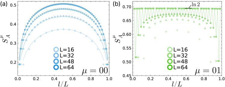
Figure S9: (a) Numerical results of $S^{\vec{\mu}}_{A}$ for $\mu=00$ in the TFIM. Data is fitted to the curve $S^{\vec{\mu}}_{A}=c_{\vec{\mu}}\ln[(L/\pi)\sin(\pi l/L)]+\text{const}$, leading to $c_{\vec{\mu}}=0.097$. The constant is the same for all four curves. (b) Numerical results of $S^{\vec{\mu}}_{A}$ for $\mu=01$.

We have also calculated the averaged swapped EE $\overline{S}_{A}$ as shown in Fig. S10. Despite the fact that the boundary conditions induced by the measurement outcomes $\mu=01$ and $\mu=11$ should not be conformally invariant, the averaged value $\overline{S}_{A}$ recovers the logarithmic scaling with $l$. Interestingly, the value of the coefficient in the logarithmic scaling is close to that of the uniform outcome case, in the same manner as in the case of the TLLs discussed in the main text.

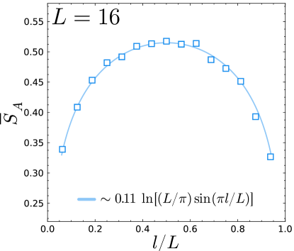
Figure S10: Numerical results of $\overline{S}_{A}$. Statistical errors are small compared to the size of the markers.

These numerical results strongly indicate that the swapped entanglement can exhibit the universal behavior also in the case of the TFIM. To understand its origin, one needs to identify the conformal boundary conditions realized by the Bell-state measurements. Here we shall give a brief discussion. Following the path-integral approach used in the main text, we can express the measurement operator $P^{\vec{\mu}}$ by the field operators. The measurement operator for $\mu=b_{1}b_{2}$ in terms of Pauli matrices reads:

$$P^{\vec{\mu}}=\lim_{g\to\infty}\frac{1}{4\cosh^{2}g}\exp[g\sum_{j=1}^{l}\quantity((-1)^{b_{2}}\sigma_{j}^{x}\sigma_{j^{\prime}}^{x}+(-1)^{b_{1}}\sigma_{j}^{z}\sigma_{j^{\prime}}^{z})\Bigr{]}.$$ (S50)

(We can add a term $-(-1)^{b_{1}+b_{2}}\sigma_{j}^{y}\sigma_{j^{\prime}}^{y}$ in the exponential, as done in the main text.) The Pauli matrices are related to the Ising CFT primary fields $\varepsilon,\sigma$ as follows:

$$\sigma_{j}^{x}-\expectationvalue*{\sigma^{x}} \sim\varepsilon,$$ (S51)

$$\sigma_{j}^{z} \sim\sigma.$$ (S52)

Here, $\expectationvalue*{\sigma^{x}}$ is the ground-state expectation value of $\sigma_{j}^{x}$. When there are two independent Ising CFTs, it can be bosonized into a single free boson $\varphi$ as follows [92, 126, 127]:

$$\varepsilon_{1}\varepsilon_{2} =(\partial_{x}\varphi)^{2}+(\partial_{\tau}\varphi)^{2},$$ (S53)

$$\varepsilon_{1}+\varepsilon_{2} =\cos(2\varphi),$$ (S54)

$$\sigma_{1}\sigma_{2} =\cos\varphi.$$ (S55)

Through this bosonization, the measurement operator can be rewritten as

$$P^{\vec{\mu}}\propto\lim_{g\to\infty}\exp\{g\int_{0}^{l}dx\int_{0}^{\beta}d\tau\delta(\tau)\Bigl{[}(-1)^{b_{2}}\quantity((\partial_{x}\varphi)^{2}+(\partial_{\tau}\varphi)^{2}+h\cos(2\varphi))+(-1)^{b_{1}}\cos\varphi\Bigr{]}\Bigr{\}}.$$ (S56)

Here, $h$ is a constant that corresponds to $\expectationvalue*{\sigma^{x}}$. This expression leads to the boundary action,

$$\delta S=-g\int_{0}^{l}dx\int_{0}^{\beta}d\tau\delta(\tau)\Bigl{[}(-1)^{b_{2}}\quantity((\partial_{x}\varphi)^{2}+(\partial_{\tau}\varphi)^{2}+h\cos(2\varphi))+(-1)^{b_{1}}\cos\varphi\Bigr{]}.$$ (S57)

Our numerical calculations indicate that if $b_{2}=0$, then the configuration that minimizes this boundary perturbation in the limit $g\to\infty$ should lead to a conformal boundary. Identifying this boundary condition as a known conformal boundary remains an open question.