Excitonic topology and quantum geometry in organic semiconductors

Abstract

Excitons drive the optoelectronic properties of organic semiconductors which underpin devices including solar cells and light-emitting diodes. We demonstrate that excitons can exhibit topologically non-trivial states and identify a family of organic semiconductors exhibiting the predicted excitonic topological phases. We also show that the topological phase can be controlled through chemical functionalisation and through the dielectric environment of the material. Appealing to quantum Riemannian geometry, we predict that topologically non-trivial excitons have a lower bound on their centre-of-mass spatial spread, which can significantly exceed the size of a unit cell. The discovery of excitonic topology and excitonic Riemannian geometry in organic materials brings together two mature fields and suggests many new possibilities for a range of future optoelectronic applications.

Introduction.— Topology is a versatile tool that drives the study of diverse condensed matter phenomena. Topological invariants arise due to phases acquired by wave functions when adiabatically transported around the Brillouin zone, and provide a classification of states of matter that has radically transformed our understanding of inorganic materials over the past few decades [1, 2]. This work has culminated in a rather complete understanding of free fermionic band structures, which can be characterised through the gluing together of eigenvalues, or irreducible representations, between high symmetry points in the momentum space Brillouin zone [3, 4, 5, 6]. Assessing whether this admits an exponentially localised Wannier representation in real space leads to their topological characterisation [7, 8]. Current efforts are moving from free fermion systems towards the question of how these ideas can drive new understanding in interacting systems. An example of an interacting system is that of electron-hole bound states, or excitons.

Excitons dominate the optoelectronic properties of a wide range of materials, particularly those made of weakly interacting organic molecules. Organic semiconductors possess excellent light-harvesting properties, driven by the formation of excitons [9, 10, 11, 12], while being chemically versatile [13, 11], cheap, and environmentally friendly to fabricate [14, 15]. These features make organic semiconductors one of the most promising material platforms in which to realise optoelectronic devices, from photovoltaics [16, 17] and light-emitting diodes [18, 19] to biosensors [20]. The electron-hole distance and the centre-of-mass location of excitons can differ greatly between materials, and delocalised excitons with high mobilities are particularly promising for applications [21].

Figure 1: Formation of topological excitons from electron and hole pairs in organic materials, induced by photoexcitation with light. Topological excitons exhibit a winding of the excitonic Bloch vectors $\ket{u^{\text{exc}}_{q}}$ as the momentum of the excitons is changed, which is captured by the excitonic Berry phases $\phi_{\text{exc}}$ and associated inversion symmetry-protected topological $\mathbb{Z}_{2}$ invariant $P_{\text{exc}}$.

In this work, we establish a link between the rich exciton phenomenology in organic semiconductors with novel topological insights of such phases, developing a promising platform in which these ideas could culminate in experimentally viable topological phases and phenomena. In particular, we fully characterise the inversion-symmetry-protected excitonic topology in one-dimensional systems in terms of the excitonic Berry phase and a $\mathbb{Z}_{2}$ excitonic topological invariant. Additionally, we derive a lower bound on the spread of the exciton centre-of-mass wavefunction arising from a non-trivial excitonic quantum metric induced by the excitonic topology.

We derive these results using model Hamiltonians and, importantly, we also predict their manifestation in the polyacene family of one-dimensional organic semiconductors. We identify material realisations of all predicted topological phases, which can be manipulated both chemically through the lateral size of the polyacene chains and externally through changes in the dielectric environment. Our findings of exotic excitonic states in organic materials bring together organic chemistry, semiconductor physics, and topological condensed matter.

Excitonic topology and Berry phases.— The topological character of excitons is fully encoded in the excitonic wavefunction $\ket{\psi^{\text{exc}}_{\textbf{q}}}$. In a periodic crystal, the excitonic wavefunction [22, 23, 24, 25] can be decomposed in terms of (i) electronic single-particle Bloch states ${\ket{\psi^{\text{e}}_{\textbf{k}}}=e^{i{\bf k}\cdot{\bf r}_{\text{e}}}\ket{u^{\text{e}}_{\textbf{k}}}}$, (ii) hole single-particle Bloch states ${\ket{\psi^{\text{h}}_{\textbf{k}}}=e^{i{\bf k}\cdot{\bf r}_{\text{h}}}\ket{u^{\text{h}}_{\textbf{k}}}}$, and (iii) an interaction-dependent envelope function $\psi_{\textbf{q}}({\bf k})$; leading to a coherent superposition of electron-hole pairs:

$$\ket{\psi^{\text{exc}}_{\textbf{q}}}=\sum_{\bf k}\psi_{{\bf q}}({\bf k})e^{i{\bf k}\cdot({\bf r}_{\text{e}}-{\bf r}_{\text{h}})}\ket{u^{\text{e}}_{\mathbf{k+q}/2}}\ket{u^{\text{h}}_{\mathbf{-k+q}/2}}.$$ (1)

We also introduce $\ket{u^{\text{exc}}_{\textbf{q}}}$ as the cell-periodic part of the excitonic Bloch state $\ket{\psi^{\text{exc}}_{\textbf{q}}}=e^{i{\bf q}\cdot{\bf R}}\ket{u^{\text{exc}}_{\textbf{q}}}$, where ${\bf R}=({\bf r}_{e}+{\bf r}_{h})/2$ is the centre-of-mass position of the exciton. Notably, the relative position ${\bf r}={\bf r}_{\text{e}}-{\bf r}_{\text{h}}$ of the electron and hole enters the excitonic state via phase factors weighted by the envelope amplitudes $\psi_{{\bf k}}(\textbf{q})$. The solutions of the single-particle electronic problem for electrons and holes, and of the Wannier equation for the envelope part, fully determine the excitonic wavefunction. The excitonic topology can then be studied from the cell-periodic part $\ket{u^{\text{exc}}_{\textbf{q}}}$, on eliminating the phase factor with the centre-of-mass momentum q coupling to the centre-of-mass position ${\bf R}$.

Consistently with K-theory [26, 5], which provides classifications that are stable up to adding an arbitrary number of trivial bands to the system, in the presence of inversion symmetry we can obtain an excitonic $\mathbb{Z}_{2}$ invariant $P_{\text{exc}}=\phi_{\text{exc}}/\pi\,\text{mod}\,2$ from a Berry phase defined in one spatial dimension [27]:

$$\phi_{\text{exc}}=\int_{\text{BZ}}\differential q~{}A_{\text{exc}}(q),$$ (2)

where $A_{\text{exc}}(q)=\mathrm{i}\bra{{u^{\text{exc}}_{q}}}\ket{\partial_{q}u^{\text{exc}}_{q}}$ is the excitonic Berry connection. Alternatively, the excitonic $\mathbb{Z}_{2}$ invariant can be re-written as [28]:

$$P_{\text{exc}}=\frac{1}{\pi}\int_{\text{hBZ}}\differential q~{}[A_{\text{exc}}(q)+A_{\text{exc}}(-q)],$$ (3)

with the integration performed over a half Brillouin zone (hBZ) because the inversion symmetry relates the excitonic bands at $q$ and $-q$. The $\mathbb{Z}_{2}$ nature of the invariant can be understood intuitively: at the inversion-symmetry-invariant momenta, $q=0$ and $q=\pi$, the excitonic eigenvectors $\ket{u^{\text{exc}}_{q}}$ have the same relative phase in the trivial excitonic regime, whereas in the topological regime these have opposite inversion eigenvalues related by a $\pi$ phase. The invariant $P_{\text{exc}}$ precisely distinguishes two different topologies which are not transversable from one to another without closing a gap in the excitonic bands, similarly to the inversion-protected topology of electrons necessitating a gap closure for a topological phase transition to occur.

Phase diagram.— To explore exciton topology in a one-dimensional setting, we consider the excitonic Wannier equation for the envelope function $\psi_{q}(k)$:

$$\sum_{k^{\prime}}h_{k,k^{\prime}}(q)\psi_{q}(k)=E(q)\psi_{q}(k),$$ (4)

where $E(q)$ is the exciton binding energy and $h_{k,k^{\prime}}(q)=(E^{e}_{k+q/2}-E^{h}_{k-q/2})\delta_{k,k^{\prime}}-W_{k,-k^{\prime},q}$ includes the single-particle energies for the electrons $E^{e}_{k+q/2}$ and holes $E^{h}_{k-q/2}$ and the electron-hole interaction $W_{k,-k^{\prime},q}$. For the single-particle electron and hole states we use the Su-Schrieffer-Heeger (SSH) model [29, 30]:

$$\begin{split}H=-t_{1}\sum_{j}c^{\dagger}_{B,j}c_{A,j}-t_{2}\sum_{j}c^{\dagger}_{{B+1},j}c_{A,j}+\text{h.c.},\end{split}$$ (5)

with $c^{\dagger}_{B,j}/c_{A,j}$ the creation/annihilation operators for the electrons at sublattices $A,B$, in unit cell $j$, and staggered hopping parameters $t_{1}$ and $t_{2}$, where we define the origin of a unit cell such that $t_{1}$ is the intracell hopping and $t_{2}$ is a hopping across the boundary of the unit cell. Importantly, we also identify a family of organic acene one-dimensional polymers as candidate materials [31, 32], to realise the predicted exciton topological phases, for which we describe the single-particle states using density functional theory [33, 34].

By numerically solving the Wannier equation, we construct the excitonic phase diagram as a function of single-particle states characterised by the hopping parameters $t_{1}$ and $t_{2}$, as shown in Fig. 2(a). The phase diagram exhibits three different regimes that are determined by the interplay between single-particle electronic and hole, and excitonic topological invariants. Additionally, we fit the Wannierised low-energy bands of multiple polyacenes to the tight-binding SSH model to identify their location on the phase diagram.

In region I, corresponding to $t_{1}>t_{2}$, we have trivial electrons and holes yielding trivial excitons. This is a consequence of the absence of winding in the vectors $\ket{u^{\text{e}}_{{\bf k}}}$ and $\ket{u^{\text{h}}_{{\bf k}}}$ that leads to a trivial electronic Berry phase with $\phi_{\text{e}}=0$ and to electronic Wannier centres localised at the centres of the unit cells [35]. In region II, corresponding to $t_{1}<t_{2}$, we have topological electrons and holes, resulting in topological excitons, whose topological character is inherited from the underlying electron and hole topology. Explicitly, we have $\phi_{\text{exc}}=\phi_{\text{e}}=\phi_{\text{h}}=\pi$, where $\phi_{\text{e}}$ and $\phi_{\text{h}}$ are single-particle Berry phases of electrons and holes, respectively. In region III, also corresponding to $t_{1}<t_{2}$, we obtain $\phi_{\text{exc}}=0$, despite the presence of non-trivial electrons and holes with $\phi_{\text{e}}=\phi_{\text{h}}=\pi$. In this regime, the electron-hole interaction is the dominant energy scale and it trivialises the excitonic topology, as explained below. Additionally, the excitons are shifted with respect to the electrons and holes constituting them [36]. Intuitively, electrons and holes from different unit cells combine to give excitons with the centre of mass in-between them, as manifested by the corresponding electron, hole, and excitonic Wannier centres given by the Zak phases (see Fig. 3).

In the phase diagram of Fig. 2(a), we indicate where polyanthracene ($N=3$) and polypentacene ($N=5$) lie, providing material realisation of both trivial and topological excitonic phases. Polyheptacene ($N=7$) also falls within region II, but it exhibits relatively flat bands with $t_{1}<0.2$ eV and therefore falls outside the range plotted in Fig. 2(a). Interestingly, the excitonic topology of the acenes can be controlled through the dielectric screening strength as illustrated for polypentacene in Fig. 2(b) and for polyheptacene in Fig. 2(c). Therefore, it should be possible to experimentally control exciton topological order by changing the dielectric environment of materials. For example, free standing polypentacene sits in the excitonic topological region II of the phase diagram, but increasing dielectric screening through a SiO₂ substrate or hBN encapsulation drives it towards the excitonic trivial phase in region III, as illustrated in Figure  2(b). In an experimental setting, the screening strength can be controlled through substrate choice, but also through chemical functionalisation and solution, providing readily available tools to explore the phase diagram in Fig. 2(a).

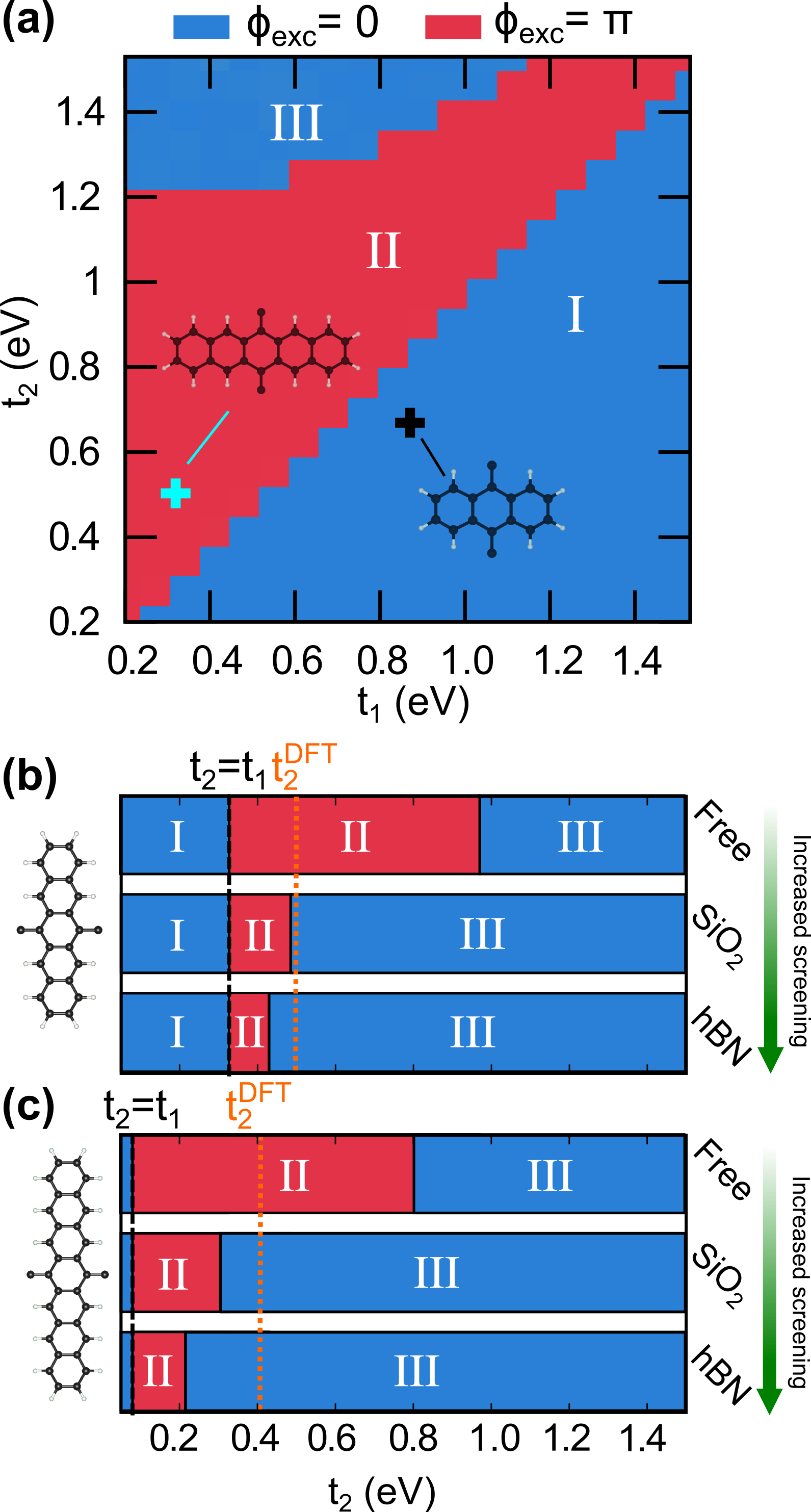
Figure 2: (a) Phase diagram showing excitonic topological phases as a function of $t_{1}$ and $t_{2}$, with $L=0.8$ nm and $\alpha_{\text{1D}}=0.05$ eVÅ. The phase regimes are defined as I, II, and III as discussed in the main text. We also indicate the location of polyanthracene (black cross) and polypentacene (cyan cross) in the phase diagram. (b,c) Phase diagram cuts for fixed $t_{1}$ for (b) polypentacene and (c) polyheptacene, on different background dielectrics. For these diagrams, we use material specific parameters $t_{1}$ and $L$ extracted from DFT, and $t_{2}$ is marked on the phase diagram with the orange dotted line.

Characterisation of topological excitons.— To gain a deeper understanding of the exciton topology and phase diagram presented in Fig. 2, we phenomenologically capture the electron-hole interaction through a dualisation picture using a SSH-Hubbard-like model with a hierarchy of electronic density-density interactions $U_{i}$, with ${i=1,2,3,\ldots}$ labelling interactions between $n^{\text{th}}$ order left neighbours for odd $i$, and right $n^{\text{th}}$ order neighbours for even $i$. We show that in the limits of vanishing interactions, as well as very high interaction strengths compared with the hopping energies, the physics is effectively captured by the above interacting SSH model either in terms of electronic degrees of freedom or in terms of “dual” density degrees of freedom.

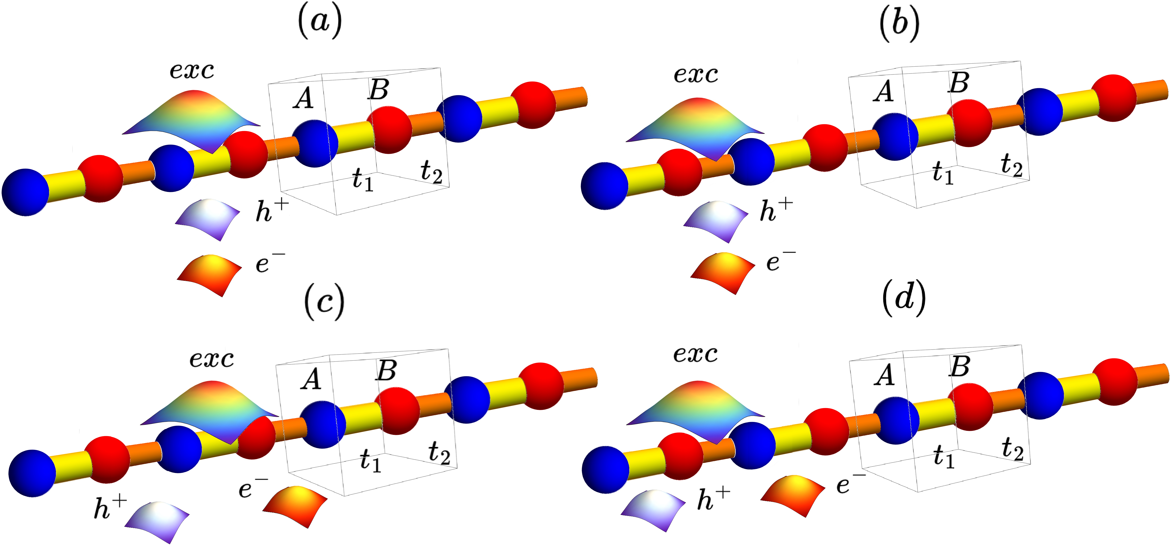
Figure 3: Real space realisation of different combinations of Wannier centre shifts corresponding to the Berry phases of electrons, holes, and excitons, with the interaction-driven mechanisms of the formation of topological and trivial excitons elucidated schematically. (a) Trivial electrons and holes forming trivial excitons ($P_{\text{exc}}=0$) in few-ring polyacenes. (b) Topological electrons and holes forming topological excitons ($P_{\text{exc}}=1$) in many-ring polyacenes. (c) Topological electrons and holes forming trivial excitons ($P_{\text{exc}}=0$) in largest-ring polyacenes with nearly-flat bands. In this case the excitons exhibit a trivialised excitonic Berry phase due to the interaction of obstructed electrons and holes shifted from the origin. (d) Topological excitons ($P_{\text{exc}}=1$) formed out of trivial electrons and holes. Cases (a)-(c) are realised in the lowest excitonic band of polyacenes, while (d) only appears for the higher excitonic bands.

To concretise this phenomenological picture for the bottom exciton band, two limits are of central importance. In the first limit, we consider an interaction smaller than the bandwidth $U_{i}\ll t_{1},t_{2}$, obtaining the standard SSH model [29, 30]. For $t_{2}<t_{1}$, we obtain vanishing Berry phases for electrons, holes, and excitons, with all of them localised at the origin of the unit cell [Fig. 3(a)], and corresponding to region I of Fig. 2. For $t_{2}>t_{1}$, and in this dispersive limit, the electrons, holes, and as a consequence, the excitons, all acquire $\pi$ Berry phases, which is also reflected by the inversion-symmetry protected shift of all with respect to the unit cell origin [Fig. 3(b)], corresponding to region II of Fig. 2.

The other limit corresponds to dominant interactions. This regime is characterised by flat bands ($t_{2}\gg t_{1}$ or $t_{2}\ll t_{1}$) and the interactions take the dominant role $U_{i}\gg t_{1},t_{2}$, for $i=1,2$. The electronic hopping terms become negligible and the nearest-neighbour interactions, modelled with the Hubbard terms, take over the role of the quasiparticle hoppings, with density operators taking the role of creation and annihilation operators after a particle-hole transformation ($h^{\dagger}_{A/B}=c_{A/B}$) and a bosonisation to the localised exciton basis (${b^{\dagger}_{A/B}=c^{\dagger}_{A/B}h^{\dagger}_{A/B}}$), as detailed in the Appendix. On relabelling the dominant nearest-neighbour interaction energies $U_{1}$ and $U_{2}$ as $2t^{\text{exc}}_{1}$ and $2t^{\text{exc}}_{2}$, the dual Hamiltonian takes an SSH form:

$$\begin{split}H=-t^{\text{exc}}_{1}\sum_{j}b^{\dagger}_{B,j}b_{A,j}-t^{\text{exc}}_{2}\sum_{j}b^{\dagger}_{{B+1},j}b_{A,j}+\text{h.c.}.\end{split}$$ (6)

Diagonalizing this effective dual Hamiltonian with excitonic states directly gives the excitonic eigenvectors $\ket{\psi^{\text{exc}}_{q}}$ without reference to the envelope function which results from the Wannier equation, and allowing us to directly compute the excitonic $\mathbb{Z}_{2}$ invariant $P_{\text{exc}}$ and the excitonic Berry phase $\phi_{\text{exc}}$.

With the dual Hamiltonian in Eq. (6), we obtain the topology of region III when $t_{2}\gg t_{1}$ and $t^{\text{exc}}_{1}>t^{\text{exc}}_{2}$, as well as the part of region I with $(t_{1}\ll t_{2})$. We stress that the rest of region I (where the bandwidth is larger than $U_{i}$) and region II are a consequence of the electronic SSH Hamiltonian in the opposite limit, where the excitons directly inherit the topology of electrons and holes, without any additional interaction-driven effects, which are negligible in these parts of the phase diagram.

The above arguments allow us to reconstruct the above limiting cases and thus the different sectors I, II, and III of the phase diagram relevant for a realistic $\mathbb{Z}_{2}$ excitonic topological organic semiconductor. We note that we do not retrieve a region with trivial electronic and hole Berry phases $(\phi_{\text{e}}=\phi_{\text{h}}=0)$ and topological excitons $\phi_{\text{exc}}=\pi$ in the lowest excitonic band. Interestingly, this regime can in principle be obtained in a similar model in the limit $U_{2}>U_{1}\gg t_{2}$, and with $t_{1}\gg t_{2}$, as demonstrated recently in Ref. [36]. However, in real materials, the single-particle parameters $t_{1}$ and $t_{2}$ and the exciton parameters $t^{\text{exc}}_{1}$ and $t^{\text{exc}}_{2}$ might not be independent, and we do not find this regime in our phase diagram in Fig. 2.

Additionally, we can utilise our model analysis to capture the phenomenology of the shifting of the boundary between region II and region III in the strong screening limit. The intuitive picture is that in the presence of a strongly polar substrate, the interaction between the electrons and holes within the organic material becomes screened, and the weakly interacting electrons and holes in different cells form excitons with the centre of mass residing centrally in-between, see Fig. 3(c). Effectively, the described pinning of the excitons is imposed by an external substrate, which we also quantitatively detail in the Appendix. As such, there is a mismatch between the Berry phases, or equivalently Wannier centre positions of the electrons and holes, known to reflect the electric polarisation associated with the charge distribution in the material [37], compared to the excitons. This culminates in the topology of region III, consistently with the numerical results. While the qualitative theoretical argument above does not require the numerical solution of the Wannier equation to deduce the topological structure of the excitonic phase diagram, a full numerical solution is however necessary to quantitatively build the topological excitonic phase diagram boundaries between regions II and III, as shown in Fig. 2.

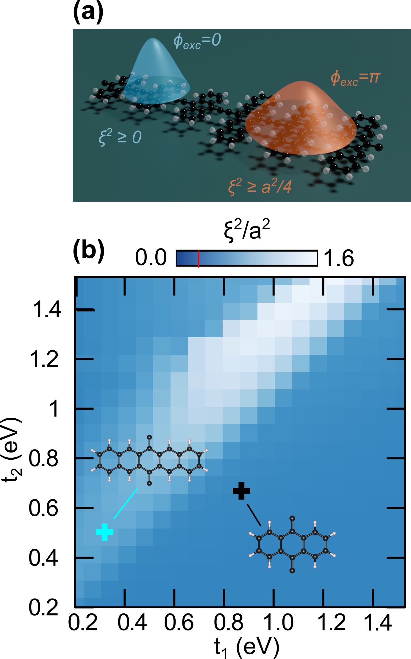
Figure 4: (a) Illustration of topological (orange) and trivial (blue) excitons in polyacenes with the corresponding excitonic Berry phases and excitonic Wannier state spreads bounded below by the excitonic quantum metric. (b) Spread of the excitonic Wannier states $\xi^{2}$ as a function of the single-particle hopping parameters $t_{1}$ and $t_{2}$, with the excitonic phase bounded by the excitonic quantum geometry (red line in gradient bar).

Excitonic quantum geometry.— The excitonic topology described above has a direct implication on a geometric property, the spread (variance) of the excitonic states in the centre-of-mass coordinate ${\bf R}$. To understand this relation, we consider the quantum metric $g_{ij}$ [38, 39], which is a tensor made of symmetrised derivatives of momentum-space Bloch states, and defined as:

$$g^{\text{exc}}_{ij}=\frac{1}{2}\Big{[}\bra{\partial_{q_{i}}u^{\text{exc}}_{\textbf{q}}}1-\hat{P}\ket{\partial_{q_{j}}u^{\text{exc}}_{\textbf{q}}}+\text{c.c.}\Big{]},$$ (7)

where $\hat{P}=\ket{u^{\text{exc}}_{\textbf{q}}}\bra{u^{\text{exc}}_{\textbf{q}}}$ is a projector onto the exciton band of interest. More generally, it can be considered to be the real part of a Hermitian quantum geometric tensor (QGT) [38, 40], which can be written as [38, 41]:

$$Q^{\text{exc}}_{ij}=\bra{\partial_{q_{i}}u^{\text{exc}}_{\textbf{q}}}1-\hat{P}\ket{\partial_{q_{j}}u^{\text{exc}}_{\textbf{q}}},$$ (8)

The imaginary part of the QGT corresponds to the Berry curvature, encoding the topology, which underlies quantum Hall phenomena, while the positive-semidefiniteness of the QGT equips the metric and the Berry curvature with a set of physical bounds related to optics, superconductivity, and quantum transport [40]. The geometric meaning of the metric can be further identified by defining a Fubini-Study metric [38] ${\differential s^{2}=1-\Big{|}\bra{u^{\text{exc}}_{\bf q}}\ket{u^{\text{exc}}_{{\bf q}+\differential{\bf q}}}\Big{|}^{2}}$ and recognizing that

$$\differential s^{2}=g^{\text{exc}}_{ij}\differential q^{i}\differential q^{j},$$ (9)

which is reminiscent of the well-known relation between the metric and the spacetime intervals in general relativity, and where the Einstein summation convention is implicitly assumed.

In the context of excitons, the metric maps to the variance of the maximally-localised excitonic Wannier functions (MLXWF) [42] in real space. In this regard, we numerically demonstrate the spread of the excitons in Fig. 4. We observe that whenever the topological excitonic invariant $P_{\text{exc}}$ is non-trivial, the diameter associated with the variance of the real space exciton wavefunctions necessarily needs to exceed the size of the unit cell due to the non-trivial topology set by the quantized Berry phase. Specifically, as illustrated in Fig. 3, we find that for an excitonic inversion invariant $P_{\text{exc}}=0$, the excitons are localised inside the unit cell at its centre and have no lower bound on their spread.

The connection between the exciton spread and the metric can be quantified by a bound set by an integral of the quantum metric, $\oint\differential q\,g^{\text{exc}}_{xx}$, where in one dimension, which we refer to as the $x$-direction, only the $g_{xx}$ component exists. Using a Cauchy-Schwartz type inequality, we find:

$$\xi^{2}\geq\frac{a^{2}P_{\text{exc}}^{2}}{4},$$ (10)

where $a$ is the unit cell length and $\xi^{2}\equiv\text{Var}\,R=\langle R^{2}\rangle-\langle R\rangle^{2}$ is the variance with respect to the MLXWF center. This relation explicitly shows that the size of topological excitons, as captured by the spread of the excitonic Wannier functions, should be comparable to, or even exceeding, the size of the unit cell, matching the numerical results. That is, topological excitons with $P_{\text{exc}}=1$ are shifted to the boundary of the unit cell $\langle R\rangle=a/2$ and their spread $\xi^{2}\equiv\text{Var}\,R=\langle R^{2}\rangle-\langle R\rangle^{2}$ is bound from below, resulting in the centre-of-mass $R$ of an exciton being localised within a characteristic length $\xi\sim a/2$. In the presence of a localised electron or hole (e.g. through defect pinning), the bound on the delocalisation of the centre-of-mass $R$ position also determines the effective size of the exciton characterised by the electron-hole distance $r$. This is consistent with the observed transition from localised “Frenkel” to spread out “Mott-Wannier” excitons in polyacenes [32]. Finally, we note that the quantum-geometric bound due to excitonic band topology persists in the higher excitonic bands, see Fig. 5. In the higher bands, quantum geometry takes a more dominant role, even without the presence of non-trivial topology, due to the contributions of alternating envelope functions of the weaker-bound higher energy excitonic states, as we describe in Appendix.

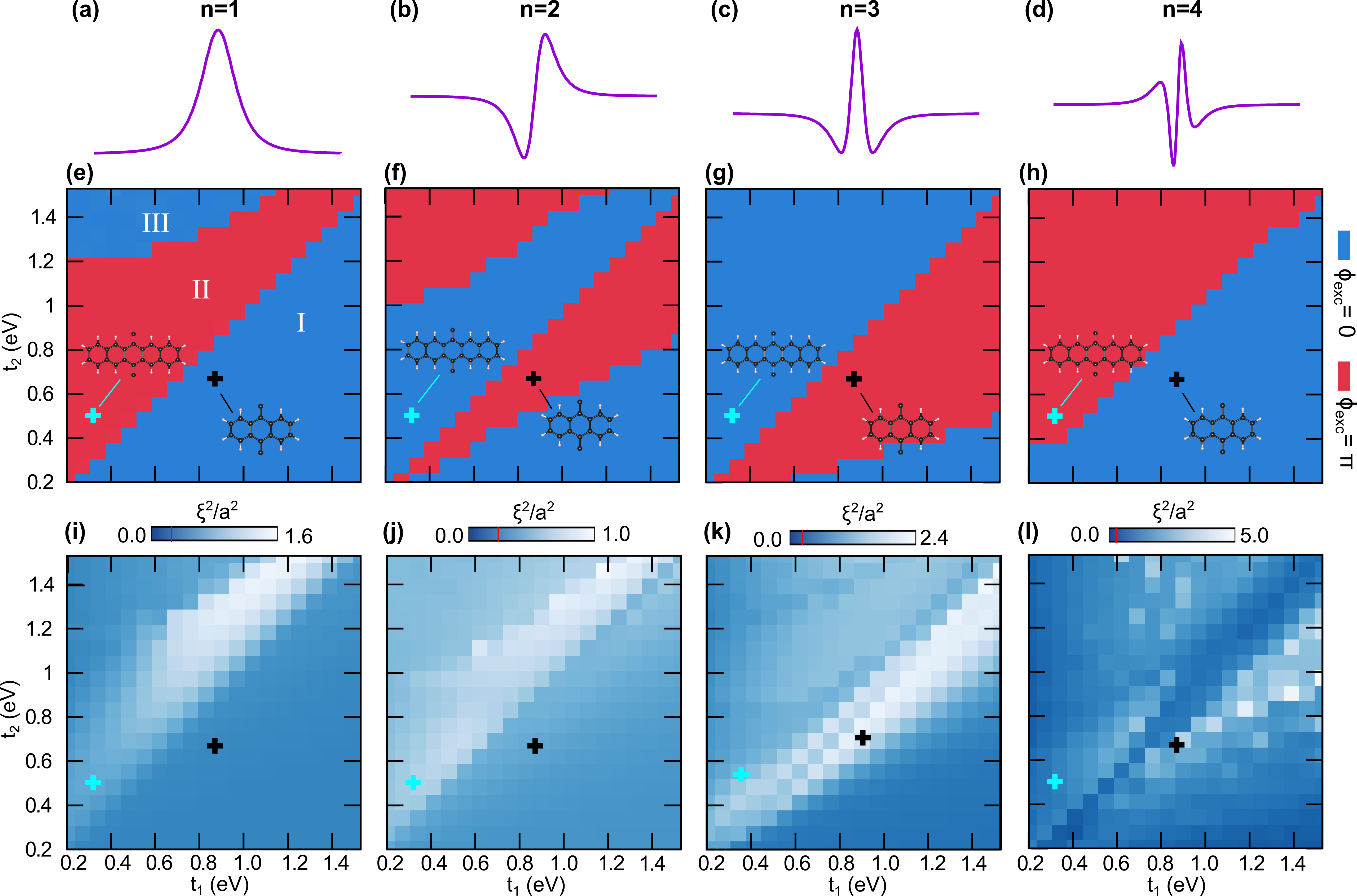
Figure 5: (a-d) Envelope functions $\psi_{q=0}(k)$ for different excitonic bands $n=1,2,3,4$, respectively. (e-h) Topological excitonic phase diagram as a function of the hopping parameters $t_{1}$ and $t_{2}$, highlighting regions with different invariant ${P_{\text{exc}}=\phi_{\text{exc}}/\pi~{}\text{mod}~{}2}$ and identifying the location of various polyacenes. The excitons in polypentacene (cyan cross) and polyheptacene (black cross) realise different excitonic topologies. (i-l) Spread of the excitonic Wannier states $\xi^{2}$, with the excitonic topological phases bounded by the excitonic quantum geometry (red line in gradient bar). Although the numerical results match the general theory and topological phase diagram intimately, we note that in higher excitonic bands $n=3,4$ (k-l) there is a larger spread in the excitonic wavefunctions due to the non-trivial quantum geometry induced by the more delocalised envelope function, even when the topology of the exciton is trivial (see main text).

Discussion.— Our findings open up multiple research avenues. From a theoretical point of view, the SSH-like topology discussed above, also referred to as obstructed insulators, is the simplest kind of topology. Extending the study of topological excitons to higher dimensional systems and to materials with different types of (crystalline) symmetries is expected to greatly expand excitonic topology and quantum geometry [24, 23, 25, 41, 36]. Another interesting research direction is to extend the discussion above to spinful systems, which would enable a distinction between singlet and triplet excitons.

Moreover, higher excitonic bands (see Fig. 5) in the studied polyacene systems also exhibit the excitonic topology and non-trivial quantum geometry. Here, the flipping of regions with $P_{\text{exc}}=0$ and $P_{\text{exc}}=1$ can be explained with the change of the shape of the excitonic envelope functions, as deduced from solving the Wannier equation. Namely, at the level of the Wannier equation, the envelope determines $U_{i}$, which in turn contribute to $\phi_{\text{exc}}$, as detailed in Appendix. For higher excitonic bands, the dualised theoretical picture still holds by the same argument as for the lowest excitonic bands, although the $U_{i}$ terms compare differently, which can change the excitonic topology and phase diagram. In particular, we note that unlike in the lowest excitonic band, a fourth region with trivial electrons and holes, but with topological excitons [36], emerges for the first higher excitonic bands ($n=2,3$), which is manifested in polyanthracene ($N=3$). Again, the dielectric screening can shift the excitonic phase diagram boundaries, showing that a modification of the substrate can also change the topology of higher excitonic bands in organic materials.

These potential theoretical extensions would naturally fit with active areas of experimental exciton research. Excitons are experimentally studied through their optical, dynamics, and transport properties, using techniques such as pump-probe experiments. The findings reported above already anticipate some potential experimental manifestations of exciton topology. First, the distinct excitonic topology exhibited by the different excitonic states (see Fig. 5) suggests that optical probes could selectively target different excitonic behaviour in the same material, as well as unusual dynamics as the excitons relax towards the lowest energy state following photoexcitation. Second, the lower bound set on the exciton size by quantum geometry (see Fig. 4) suggests that transport will be enhanced for topological excitons compared to their trivial counterparts. Third, a hallmark of topology is the so-called bulk-boundary correspondence, in which the bulk topology is associated with unusual boundary states that are often protected against scattering and support dissipationless transport. In the case of excitons, these boundary states should be manifested in terms of dipole currents.

From the materials point of view, the interplay between topology, excitons, and organic polyacenes reported above is only the starting point. Organic semiconductors provide a more general platform to explore exciton topology, with organic semiconductors in one, two, and three dimensions often exhibiting strongly bound excitons. Additionally, it should be possible to harness the decades of experience in organic chemistry to manipulate organic semiconductors to explore many potential different excitonic topological regimes, such as those described above (Fig. 2), but notably also richer topologies in higher dimensions. Beyond organic semiconductors, inorganic two-dimensional materials and van der Waals bonded layered materials also exhibit strongly bound excitons, providing additional materials platforms to explore excitonic topology.

Conclusions.— Overall, we establish a connection between topological ideas, common in the study of electronic phases, and the field of excitons in organic semiconductors. We describe a simple proof-of-principle for exciton topology in the form of one dimensional winding numbers, constructing a full exciton topology phase diagram with different regimes reflecting the interplay between the underlying (so-called obstructed) electron and hole topologies with the new exciton topology. We also present a family of organic polymers that host the predicted exciton topologies, and demonstrate the manipulation of this topology by controlling the dielectric screening through substrate choice. Finally, we discover that exciton topology is related to the spatial localisation of excitons, as determined by Riemannian metric identities. In particular, we find a lower bound on the exciton size for topologically non-trivial excitons. Our results set a benchmark for a potentially rich exploration of topological excitons in organic semiconductors and beyond.

Appendix

.1 First principles calculations

We perform density functional theory calculations using the Quantum Espresso package [43, 44] to study a family of polyacene chains. We use kinetic energy cutoffs of $80$ Ry and $500$ Ry for the wavefunction and charge density, respectively, and $12$ $k$-points to sample the Brillouin zone along the periodic direction. We use GGA (PBE) norm-conserving pseudopotentials which were generated using the code ONCVPSP (Optimized Norm-Conserving Vanderbilt PSeudoPotential) [45] and can be found online via the Schlipf-Gygi norm-conserving pseudopotential library [46]. We impose a vacuum spacing of $34.3$ Å in the planar direction perpendicular to the polymer chain, and a vacuum spacing of $27.52$ Å in the out-of-plane direction, to minimise interactions between periodic images of the polyacene chains. We perform a structural optimisation of the internal atomic coordinates to reduce the forces below $0.0015$ Ry/Å.

We calculate the band structures of several polyacenes, as shown in Fig. 6. The hopping parameters of the SSH tight-binding model were deduced from these calculations. The SSH sites, $A$ and $B$, on the molecular unit cell are illustrated with the red and blue boxes in Fig. 6(d), with the $t_{1}$ hopping between them and the $t_{2}$ hopping across the carbon link between unit cells [31]. While we do not employ GW calculations in our work, we note that the phase diagram in Fig. 2 would be quantitatively the same, and only the position of the individual molecules on the phase diagram could differ. In particular, it was found in previous works using GW [32] that the transition from trivial to topological electrons and holes could occur between the polypentacene ($N=5$) and polyheptacene ($N=7$) polymers, in contrast with our and previous [31] calculations, where the transition occurs between $N=3$ and $N=5$.

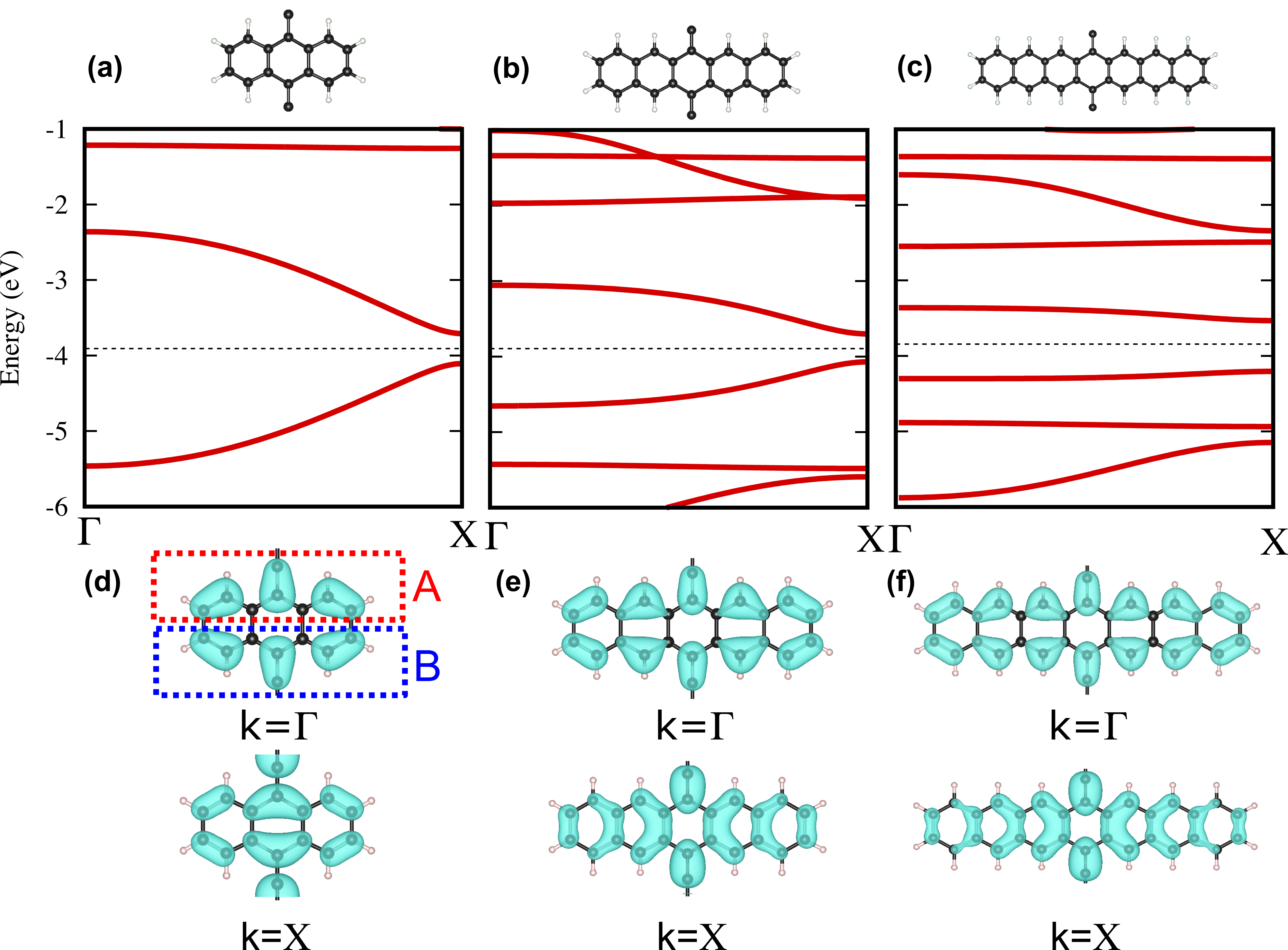
Figure 6: Electronic bands in (a) polyanthracene, (b) polypentacene, and (c) polyheptacene, calculated using DFT. (d-f) Plots of the electronic wavefunctions for the valence band in the polyacenes. The shift of the charge centre, as well as the change of the parity of the wavefunction, as indicated by the inversion symmetry eigenvalues (on changing $P_{\text{exc}}=0$ to $P_{\text{exc}}=1$) can be directly observed in the DFT result. The approximate $A$ and $B$ sublattice sites in the molecular unit cells are marked with the red and blue boxes, respectively.

.2 Wannier equation

We obtain the excitonic wavefuncions and associated bands by combining the electronic and hole states from the first principles DFT calculations with the envelope part of the excitonic wavefunction obtained by solving the Wannier equation.

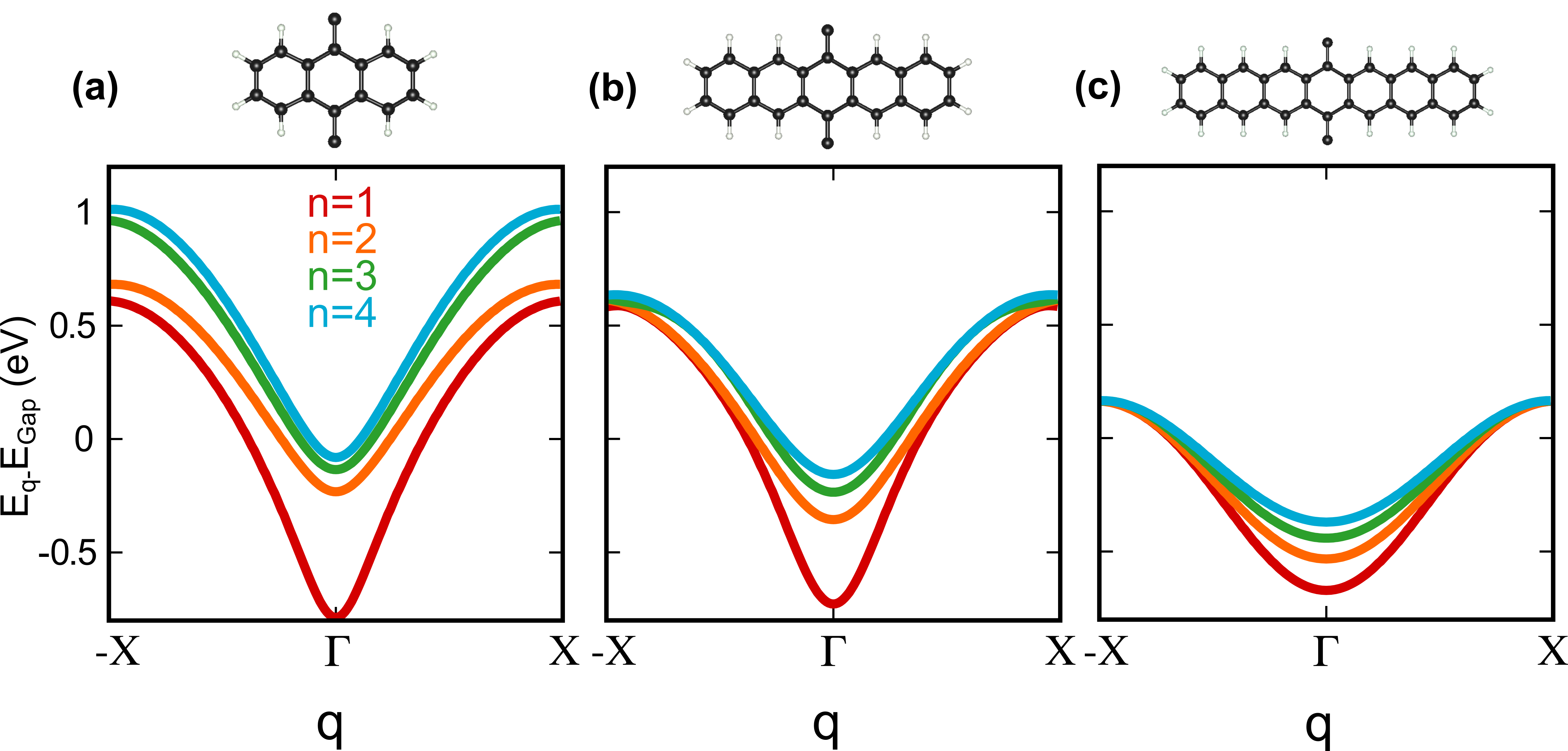
Figure 7: Excitonic bands obtained from DFT single-particle states and the solution of the Wannier equation for the envelope function. We show the dispersion of the excitonic bands $n=1,2,3,4$ of (a) polyanthracene ($N=3$), (b) polypentacene ($N=5$), and (c) polyheptacene ($N=7$). The excitonic bands are manifestly inversion-symmetric, while the excitonic bandwidths and dispersion decrease with increasing number of rings $N$ in the monomers. We also note that as the excitonic bands approach the zero energy level, they merge into the continuum of electronic energies.

We construct the electronic SSH Hamiltonian by Wannierising the electronic bands, from which $t_{1}$ and $t_{2}$ can be directly extracted. For each pair ($t_{1},t_{2}$) we solve the Wannier equation:

$$\sum_{k^{\prime}}h_{k,k^{\prime}}(q)\psi^{n}_{q}(k)=E_{n}(q)\psi^{n}_{q}(k),$$ (11)

where $\psi^{n}_{q}(k)$ is the envelope function of the $n$-th excitonic band. Moreover,

$$h_{k,k^{\prime}}(q)=(E^{e}_{k+q/2}-E^{h}_{k-q/2})\delta_{k,k^{\prime}}-W_{k,-k^{\prime},q},$$ (12)

with electron/hole energies $E^{e(h)}=E_{+(-)}$, and the interaction matrix defined as:

$$W_{k,-k^{\prime},q}= V_{\text{NR}}(k-k^{\prime})\sum_{i,j\in\{A,B\}}\varphi^{*}_{i,k+q/2}\varphi^{*}_{j,k-q/2}\varphi_{j,k+q/2}\varphi_{i,k-q/2},$$

where $\varphi_{i,k}$ is the wavefunction amplitude from the SSH model on site $i$ with momentum $k$, and $V_{\text{NR}}$ is the Coulomb potential for a one-dimensional system that describes the dielectric screening (see next Section for further details). We include the excitonic band dispersions for the lowest four excitonic bands $E_{n}(q)$ of different polyacenes, as addressed in the main text, see Fig. 7.

.3 Dielectric screening model

The Wannier equation is highly dependent on the dielectric screening, where an accurate screening model is paramount to adequately capture the excitonic physics. In the polyacene chains, the Coulomb potential corresponds to that of one-dimensional nanoribbons, and following Ref. [47] and solving Poisson’s equation, we arrive at the following form of the Coulomb potential:

$$V_{\text{NR}}(q)=\dfrac{e_{0}^{2}}{4\pi\epsilon_{0}}\dfrac{K_{0}(qL/2)}{\epsilon_{s}+8q^{2}\alpha_{\text{1D}}K_{0}(qL/2)},$$ (13)

where $L$ is the width of the ribbon, $\alpha_{\text{1D}}$ is the screening parameter (polarisability per unit length), $\epsilon_{s}$ is the background screening, and $K_{0}$ is a modified Bessel function of the second kind. We take $L$ to be the lateral size of the polyacene ribbon and fix $\alpha_{\text{1D}}=0.05$ nm${}^{-}2$ following previous work [47]. For small $q$, corresponding to long range interactions, the screening is dominated by the environment as determined by $V_{\text{NR}}(q\rightarrow 0)\sim-\log(qL/2)/\epsilon_{s}$. At large $q$, corresponding to short distances, the screening is approximately $V_{\text{NR}}(q\rightarrow 0)\sim 1/(\alpha_{\text{1D}}q^{2})$, resembling the Coulomb interaction in bulk systems. The background screening $\epsilon_{s}$, defined as the average of the dielectric above and below the organic layer, further modulates the Coulomb interaction. We consider common background dielectrics in this work: vacuum (${\epsilon_{s}=1}$), SiO₂ substrate ($\epsilon_{s}$= 2.45), and hBN encapsulation ($\epsilon_{s}$= 4.5) [48].

.4 Numerical excitonic Berry phases

To evaluate the excitonic Berry phases, we use a discretisation of the Brillouin zone $q=\left[q(1),q(2),\ldots,q(N_{q})\right]$, where we choose $q(1)=0$ and $q(N_{q})=2\pi/a-\Delta q$, with lattice parameter $a$ and grid spacing $\Delta q=2\pi/(N_{q}a)$. We use the parallel-transport gauge to numerically evaluate the Berry phase given by Eq. (2), following Ref. [49]:

$$\phi_{\text{exc}}=-\mathfrak{Im}~{}\text{log}\Big{[}\bra{u^{\text{exc}}_{q(1)}}\ket{u^{\text{exc}}_{q(2)}}\ldots\bra{u^{\text{exc}}_{q(N_{q})}}\ket{u^{\text{exc}}_{q(1)}}\Big{]}.$$ (14)

We use a $q$-grid of size $N_{q}=400$, with convergence within a numerical error of $\Delta\phi_{\text{exc}}\sim 10^{-3}$ for the excitonic Berry phase obtained above $N_{q}=200$.

.5 Decomposition of the excitonic Berry connection

To compute the excitonic invariant $P_{\text{exc}}$, we utilise Eq. (1) and decompose the excitonic Berry connection of Eq. (2) into an envelope part and a single-particle part as:

$$A_{\text{exc}}(q)=A_{\text{exc}}^{\text{en}}(q)+A_{\text{exc}}^{\text{sp}}(q).$$ (15)

The envelope part reads:

$$A_{\text{exc}}^{\text{en}}(q)=\mathrm{i}\sum_{k}\psi^{\ast}_{q}(k)\partial_{q}\psi_{q}(k),$$ (16)

and the single-particle part consists of the electron and hole contributions:

$$A_{\text{exc}}^{\text{sp}}(q)=\frac{1}{2}\sum_{k}|\psi_{q}(k)|^{2}\left[A^{\text{e}}(k+q/2)+A^{\text{h}}(k-q/2)\right].$$ (17)

In turn, the single-particle electron and hole Berry connections are given by $A^{\text{e}/\text{h}}(k\pm q/2)=\mathrm{i}\bra{u^{\text{e}/\text{h}}_{k\pm q/2}}\ket{\partial_{q}u^{\text{e}/\text{h}}_{k\pm q/2}}$.

We find that in the hopping and interaction regimes realised by the organic materials in regions I and II, the contribution to $\phi_{\text{exc}}$ due to the envelope part $A_{\text{exc}}^{\text{en}}(q)$ vanishes, whereas the single-particle contribution $A_{\text{exc}}^{\text{sp}}(q)$ due to the band geometry of the constituent electrons and holes (see “Riemmanian geometry of excitons” below), gives $\phi_{\text{exc}}=\pi$ on integrating. However, in the limit of flat bands (region III), we find that $A_{\text{exc}}^{\text{en}}(q)$ can provide an additional Berry phase contribution of $\pi$, trivialising the $P_{\text{exc}}$ invariant. To explain such change explicitly, we thus detail an analytical argument for the previously numerically found trivialisation in the lowest exciton band, which we obtain by constructing a dualisation of an interacting SSH model in the flat-band limit [36] (see “Dualisation of the interacting Hamiltonian” below).

Moreover, beyond the numerical evaluation of the excitonic Berry phase and the dualisation argument detailed further below, we analytically model the topology of excitonic wavefunctions within the phase diagram by asserting an effective form of the excitonic envelope function. Explicitly, the exciton envelope function for the $t_{2}>t_{1}$ regime, obtained by a qualitative fit to the Wannier equation solution, reads:

$$\psi_{q}(k)=\mathcal{N}\Big{[}\cos(k+q)e^{-(k+q/2)^{2}/2}+\cos(k-q)e^{-(k-q/2)^{2}/2}\Big{]},$$ (18)

with the normalisation constant $\mathcal{N}$. With this expression, we obtain a vanishing envelope contribution ${\oint\differential q~{}A^{\text{en}}_{\text{exc}}(q)=0}$, so that the excitonic topology is determined by the topology of the underlying electron and hole states.

For $t_{2}\gg t_{1}$, we interestingly obtain $\oint\differential q~{}A^{\text{en}}_{\text{exc}}(q)=\pi$, from an envelope function which was plotted in Fig. 8, a result we rationalise in the following theoretical modelling.

.6 Theoretical model

In this section we expand on the effective model discussed in the main text. We begin by building an electronic effective theoretical model based on the one-dimensional SSH Hamiltonian [29, 30]. We write Eq. (5) of the main text in the momentum-space Bloch orbital basis by introducing $c^{\dagger}_{Ak}/c_{Bk}$, on Fourier transforming the electronic creation and annihilation operators in the position basis $c^{\dagger}_{Ak}=\frac{1}{\sqrt{L}}\sum_{j=1}e^{\mathrm{i}k(r_{\mathrm{e}})_{j}}c^{\dagger}_{A,j}$,

$$H=\sum_{k;\alpha,\beta=A,B}\left[H^{\text{SSH}}(k)\right]_{\alpha\beta}c^{\dagger}_{\alpha k}c_{\beta k}.$$ (19)

with the electron position operator $(r_{\mathrm{e}})_{j}=ja$. In this basis, we have a Bloch Hamiltonian matrix which reads,

$$H^{\text{SSH}}(k)={\bf d}(k)\cdot\bm{\sigma},$$ (20)

where ${\bf d}(k)=(t_{1}+t_{2}\sin k,t_{2}\cos k,0)^{T}$, with $\bm{\sigma}=(\sigma_{x},\sigma_{y},\sigma_{z})$ the vector of Pauli matrices. The hopping parameters $t_{1}$ and $t_{2}$ can be retrieved to describe specific polyacenes by fitting them to the associated first principles calculations after Wannierisation. In this electronic model, the wavefunctions of electrons and holes take the compact form ${\ket{u^{\text{e}/\text{h}}_{k}}=\frac{1}{\sqrt{2|{\bf d}|^{2}}}({d_{x}}\pm\mathrm{i}{d_{y}},|d|)^{\text{T}}}$.

Having set up the electronic problem, we now elaborate on a theoretical model for the interaction-dependent excitonic topology. We start with a SSH-Hubbard-type model with up to the $n^{\text{th}}$ neighbor interactions $U_{i}$, with $i=1,2,3,\ldots,n$ in real space:

$$H=\sum_{j}\epsilon_{A}n_{A,j}+\sum_{j}\epsilon_{B}n_{B,j}-t_{1}\sum_{j}c^{\dagger}_{A,j}c_{B,j}+\text{h.c.}-t_{2}\sum_{j}c^{\dagger}_{A,j+1}c_{B,j}+\text{h.c.}$$ (21)

$$+\sum_{j}U_{A}n_{A,j}(n_{A,j}-1)+\sum_{j}U_{B}n_{B,j}(n_{B,j}-1)+\frac{1}{2}\sum_{j}\sum_{\alpha,\beta=A,B}\sum^{n}_{i=1}\Big{[}U^{\alpha\beta}_{2i-1}n_{\alpha,j-i}n_{\beta,j}+U^{\alpha\beta}_{2i}n_{\alpha,j+i}n_{\beta,j}\Big{]},$$

where the density operator reads, $n_{A,j}=c^{\dagger}_{A,j}c_{A,j}$, and within the tight-binding approximation for the Wannierised DFT-bands of the materials, we set the onsite energies to vanish, $\epsilon_{A}=\epsilon_{B}=0$. Similarly, the onsite interaction terms of strength $U_{A}$, $U_{B}$ vanish in a spin-polarised model, as no self-interactions should be included.

.7 Dualisation of the interacting Hamiltonian

To reflect the physics of the (screened) density-density interactions, we truncate the long-range interaction expansion at the level of the nearest-neighbor interactions $U_{1}\equiv U^{AB}_{1}$ and $U_{2}\equiv U^{AB}_{2}$ [36], assuming that $U_{1},U_{2}\gg U_{i>2}$. In the limit $t_{1},t_{2}\gg U_{1},U_{2}$, we obtain the standard SSH model for electronic bands, and $\oint\differential q\,A^{\text{en}}_{\text{exc}}(q)=0$. In this case, the entire contribution to excitonic topology can only emerge from the electrons and holes $\oint\differential q~{}A^{\text{sp}}_{\text{exc}}(q)=\pi$. Intuitively, this corresponds to the formation of excitons on the same site where the constituent electrons and holes reside.

In the opposite limit, $U_{1},U_{2}\gg t_{1},t_{2}$, the Hamiltonian reduces to:

$$\begin{split}H=\frac{U_{1}}{2}\sum_{j}[n_{A,j}n_{B,j}+n_{B,j}n_{A,j}]+\frac{U_{2}}{2}\sum_{j}[n_{A,j+1}n_{B,j}+n_{B,j}n_{A,j+1}]\end{split}$$ (22)

Notably, we recognise that $n_{B,j}=c^{\dagger}_{B,j}c_{B,j}=c^{\dagger}_{B,j}h^{\dagger}_{B,j}\equiv b^{\dagger}_{B,j}$, where $h^{\dagger}_{B,j}$ is a creation operator for a hole, and in combination with the creation operator of an electron $c^{\dagger}_{B,j}$, gives a localised exciton creation operator $b^{\dagger}_{B,j}$. Similarly, for sites $A$ we write: $n_{A,j}=c^{\dagger}_{A,j}c_{A,j}=h_{A,j}c_{A,j}\equiv b_{A,j}$. On relabelling $\frac{U_{1/2}}{2}\rightarrow-t^{\text{exc}}_{1/2}$, we obtain a dualised SSH Hamiltonian for excitons:

$$\begin{split}H=-t^{\text{exc}}_{1}\sum_{j}b^{\dagger}_{B,j}b_{A,j}+\text{h.c.}-t^{\text{exc}}_{2}\sum_{j}b^{\dagger}_{{B+1},j}b_{A,j}+\text{h.c.},\end{split}$$ (23)

where the Hubbard interactions between the electrons and holes on different sites effectively drive exciton hopping, or, in other words, exciton delocalisation. Notably, as $t^{\text{exc}}_{1/2}$ are not independent from the electronic $t_{1/2}$, we observe no pocket where topological excitons would be obtained in the lowest excitonic band from trivial electrons and holes in [36] in the phase diagram, which would correspond to an additional region IV. The reason for the lack of such independence in the real material context (unlike in an abstract tight-binding model construction) is that both $t_{1/2}$ and $U_{1/2}$ are given by the matrix elements of the same Wannier states and local Hamiltonians, as well as (Coulomb) interaction potentials, and are therefore not independent. It should be noted here that the interactions manifestly do $not$ break the inversion symmetry, by construction of the model.

Solving the excitonic Hamiltonian in region III for the eigenvectors $\ket{\psi^{\text{exc}}_{q}}$ directly gives the SSH model eigenfunctions and associated Berry phases from the dualisation. As long as $U_{2}>U_{1}\gg t_{2}\gg t_{1}$, the eigenvectors $\ket{u^{\text{exc}}_{q}}$ host an excitonic Berry phase $\phi_{\text{exc}}=\pi$ (or equivalently, for $U_{1}>U_{2}\gg t_{2}\gg t_{1}$, $\phi_{\text{exc}}=0$), independent from the electronic topology, as directly follows from the dualisation in the given flat-band limit. Hence, as the screening or $t_{2}$ change, which abruptly changes $U_{1}$ in the considered system, the $\phi_{\text{exc}}=\pi$ due to $t_{2}\geq t_{1}$, as contributed by $A^{\text{sp}}_{\text{exc}}$ reduces to $\phi_{\text{exc}}=0$ with the increasing interaction. In particular, this crossover corresponds to the regime of the applicability of the limit for the retrieved dualisation, from which explicitly $\phi_{\text{exc}}=0$ follows.

.8 Topology in the strongly-polarised screening limit

Importantly, in the studied experimentally relevant organic systems, $U_{1},U_{2}$ can be controlled by screening, but $U_{2}$ might be significantly lower than $U_{1}$ ($U_{1}\gg U_{2}$) due to the chemistry of the material. Hence, in this setting only one part of the dualised-SSH phase diagram can be accessed. As a result, only a reduction to $\phi_{\text{exc}}=0$ can be achieved with the interactions in the present case. In case all parameters could be tuned freely, however, one could consider the case where $U_{2}$ dominates $U_{1}$, which will achieve $\phi_{\text{exc}}=\pi$. This would yield topological excitons (in the lowest excitonic band) with trivial electrons and holes. This interesting scenario was recently pointed out in Ref. [36].

We now further consider the strongly-polarised limit when the screening is high, which drives an extension of the region III, with its boundary shifting such as when region II shrinks, see Fig. 2 of the main text. In particular, we provide further details on modelling and understanding the mismatch of electronic/hole, and excitonic Berry phases in that limit.

We begin by noting that in the limit of weak screened interactions, a photoexcitation introduces an electron-hole pair, by changing a population of two bands at given $k$-point, i.e. $f_{nk}=1\rightarrow 0$ in the originally occupied band $n$, and $f_{mk}=0\rightarrow 1$ at a given $k$-point in a zero-temperature limit. Any photoexcitation changes the polarisation in conduction and valence bands, as follows from the King-Smith-Vanderbilt formula within the modern theory of polarisation [37],

$$P_{c/v}=-e\int_{\text{BZ}}\frac{dk}{2\pi}~{}f_{n/mk}\mathrm{i}\bra{u_{n/mk}}\ket{\partial_{k}u_{n/mk}}=-\frac{e}{a}\bar{w}_{n/mk},$$ (24)

which additionally relates the polarisation in the conduction $(P_{c})$ or valence $(P_{v})$ bands to the Wannier centres corresponding to these bands $\bar{w}_{n,m}$. In the context of electronic and hole Wannier centres, we have $\bar{w}_{e}=\bar{w}_{n}$ and $\bar{w}_{h}=\bar{w}_{m}$. Here, the electron/hole Wannier centers are defined as [49]

$$\bar{w}_{e/h}=\bra{w^{e/h}_{0}}r_{e/h}\ket{w^{e/h}_{0}},$$ (25)

with the corresponding Wannier states obtained by Fourier-transforming electron and hole bands [49],

$$\ket{w^{e/h}_{0}}=\frac{a}{2\pi}\int_{\text{BZ}}\differential k~{}e^{\mathrm{i}kr_{e/h}}\ket{u^{e/h}_{k}}.$$ (26)

On the other hand, the excitonic Wannier center,

$$\bar{w}_{\text{exc}}=\bra{w^{\text{exc}}_{0}}R\ket{w^{\text{exc}}_{0}},$$ (27)

is defined with the excitonic Wannier states,

$$\ket{w^{\text{exc}}_{0}}=\frac{a}{2\pi}\int_{\text{BZ}}\differential q~{}e^{\mathrm{i}qR}\ket{u^{\text{exc}}_{q}},$$ (28)

which are also pictorially represented in Fig. 3. Additionally, the relation between Berry phases and the Wannier centres gives $\phi_{e/h}=2\pi\bar{w}_{e/h}/a$, which obtains the Berry phases for electron and holes. To obtain the Berry phase of the excitons $\phi_{\text{exc}}=2\pi\bar{w}_{\text{exc}}/a$ in the region III of the topological excitonic phase diagram, the Wannier equation is numerically solved. There, we numerically find $\bar{w}_{e/h}=\frac{a}{2}$ for the fully occupied/unoccupied electron/hole band, alongside $\bar{w}_{\text{exc}}=0$ for the lowest excitonic polyacene (polypentacene, with the number of rings in the monomer $N=5$, and polyheptacene, with $N=7$) bands, which can be understood as induced by pinning the electrons and holes across the unit cell with a strongly polar substrate (while respecting the inversion symmetry), such that the excitonic centre of mass $R$ coincides with the origin of the unit cell $\bar{w}_{\text{exc}}=0$.

Figure 8: (a) Excitonic envelope function for $t_{2}>t_{1}$. There is no discontinuous change of $\psi_{q}(k)$ as a function of $q$, yielding a vanishing contribution of $A^{\text{en}}_{\text{exc}}$ to $\phi_{\text{exc}}$. In this regime, the topology of excitons is given purely by the topology of constituent electrons and holes, with electron and hole and exciton Wannier centres coinciding: $\langle r_{e}\rangle=\langle r_{h}\rangle=\langle R\rangle$. (b) Excitonic envelope function for $U_{2}\gg t_{2}\gg t_{1}$, the flat band limit. In this case, $A^{\text{en}}_{\text{exc}}$ contributes $\Delta\phi_{\text{exc}}=\pi$, with electrons and holes shifted relative to the exciton centre, i.e. $\langle r_{e}\rangle=0$, $\langle r_{h}\rangle=a$, $\langle R\rangle=a/2$, respectively. Here, two Dirac-delta-like functions develop out of a single peak, and correspondingly in real space we have $\psi_{q}(r)\sim~{}\cos(\frac{\pi}{a}r)$ on Fourier transforming, which shows that for a given $q$, the electron-hole separation $r=r_{e}-r_{h}=a$ peaks at the length of the size of the unit cell, whereas, as a consequence, the probability density of finding the exciton center-of-mass is modulated periodically, and peaks at $R=a/2+ka$, with $k\in\mathbb{Z}$, where the excitonic Wannier centres are present.

.9 Riemannian geometry of excitons

In this section, we further elaborate on the Riemannian structure of the Bloch bundles of the excitonic wavefunctions and the associated excitonic quantum metric. We start by recognizing that we can equip a set, or bundle, of excitonic states $\ket{u^{\text{exc}}_{\textbf{q}}}$ with a Hermitian metric, known otherwise as a quantum-geometric tensor (QGT). Explicitly, we write [41]:

$$Q^{\text{exc}}_{ij}=\bra{\partial_{q_{i}}u^{\text{exc}}_{\textbf{q}}}1-\hat{P}\ket{\partial_{q_{j}}u^{\text{exc}}_{\textbf{q}}},$$ (29)

where $\hat{P}=\ket{u^{\text{exc}}_{\textbf{q}}}\bra{u^{\text{exc}}_{\textbf{q}}}$ is a projector onto the exciton band of interest. The excitonic QGT can be decomposed in terms of Riemannian (real) and symplectic (imaginary) parts. The imaginary part defines an excitonic Berry curvature, which can be non-trivial only in two- or higher-dimensional systems, whereas the real part defines an excitonic Riemannian metric $g^{\text{exc}}_{ij}\equiv\mathfrak{Re}~{}Q^{\text{exc}}_{ij}$, which can be non-vanishing even in one-dimensional systems.

The metric defined as the real part of the QGT explicitly reads:

$$g^{\text{exc}}_{ij}=\frac{1}{2}\left[\bra{\partial_{q_{i}}u^{\text{exc}}_{\textbf{q}}}\hat{Q}\ket{\partial_{q_{j}}u^{\text{exc}}_{\textbf{q}}}+\bra{\partial_{q_{j}}u^{\text{exc}}_{\textbf{q}}}\hat{Q}\ket{\partial_{q_{i}}u^{\text{exc}}_{\textbf{q}}}\right],$$ (30)

where $\hat{Q}=1-\hat{P}$. In the one-dimensional case, which we consider in this work, there exists a single excitonic metric component of interest:

$$\begin{split}g^{\text{exc}}_{xx}=\frac{1}{2}\Big{[}\bra{\partial_{q_{x}}u^{\text{exc}}_{q_{x}}}\ket{\partial_{q_{x}}u^{\text{exc}}_{q_{x}}}-\bra{\partial_{q_{x}}u^{\text{exc}}_{q_{x}}}\ket{u^{\text{exc}}_{q_{x}}}\bra{u^{\text{exc}}_{q_{x}}}\ket{\partial_{q_{x}}u^{\text{exc}}_{q_{x}}}+\text{c.c.}\Big{]}\\ =\bra{\partial_{q_{x}}u^{\text{exc}}_{q_{x}}}\ket{\partial_{q_{x}}u^{\text{exc}}_{q_{x}}}-\bra{\partial_{q_{x}}u^{\text{exc}}_{q_{x}}}\ket{u^{\text{exc}}_{q_{x}}}\bra{u^{\text{exc}}_{q_{x}}}\ket{\partial_{q_{x}}u^{\text{exc}}_{q_{x}}}.\end{split}$$ (31)

We note that, on taking normalised eigenvectors $\bra{u^{\text{exc}}_{\textbf{q}}}\ket{u^{\text{exc}}_{\textbf{q}}}=1$, and using the identity $0=\partial_{q}(\bra{u^{\text{exc}}_{\textbf{q}}}\ket{u^{\text{exc}}_{\textbf{q}}})=\bra{u^{\text{exc}}_{\textbf{q}}}\ket{\partial_{q}u^{\text{exc}}_{\textbf{q}}}+\bra{\partial_{q}u^{\text{exc}}_{\textbf{q}}}\ket{u^{\text{exc}}_{\textbf{q}}}$, we obtain $\bra{u^{\text{exc}}_{\textbf{q}}}\ket{\partial_{q}u^{\text{exc}}_{\textbf{q}}}=-\bra{\partial_{q}u^{\text{exc}}_{\textbf{q}}}\ket{u^{\text{exc}}_{\textbf{q}}}$. Hence, in the one-dimensional case of interest, and taking $q\equiv q_{x}$, i.e. dropping $x$-index for simplicity, we can also write,

$$g^{\text{exc}}_{xx}=\bra{\partial_{q}u^{\text{exc}}_{q}}\ket{\partial_{q}u^{\text{exc}}_{q}}-A_{\text{exc}}A_{\text{exc}},$$ (32)

where $A_{\text{exc}}=\mathrm{i}\bra{u^{\text{exc}}_{q}}\ket{\partial_{q}u^{\text{exc}}_{q}}$.

In general, the exciton quantum metric can be decomposed as:

$$g^{\text{exc}}_{ij}({\bf q})=g^{\text{en}}_{ij}({\bf q})+g^{\text{sp-en}}_{ij}({\bf q})+g^{\text{sp}}_{ij}({\bf q}),$$ (33)

with the envelope contribution:

$$g^{\text{en}}_{ij}({\bf q})=\frac{1}{2}\sum_{{\bf k}}[\partial_{q_{j}}\psi^{*}_{\bf q}({\bf k})\partial_{q_{i}}\psi_{\bf q}({\bf k})+\partial_{q_{i}}\psi^{*}_{\bf q}({\bf k})\partial_{q_{j}}\psi_{\bf q}({\bf k})]-A^{\text{en},i}_{\text{exc}}A^{\text{en},j}_{\text{exc}},$$ (34)

the single-particle contribution:

$$g_{ij}^{\text{sp}}({\bf q})=\frac{1}{4}\sum_{{\bf k}}|\psi_{\bf q}({\bf k})|^{2}\Big{[}g_{ij}^{\text{e}}({\bf k}+{\bf q}/2)+g_{ij}^{\text{h}}({\bf k}-{\bf q}/2)\Big{]}-A^{\text{sp},i}_{\text{exc}}A^{\text{sp},j}_{\text{exc}},$$ (35)

and the mixed single-particle/envelope term:

$$g_{ij}^{\text{sp-en}}({\bf q})=\frac{1}{2}\sum_{{\bf k}}\Big{[}\partial_{q_{i}}|\psi_{\bf q}({\bf k})|^{2}\partial_{q_{j}}A^{\text{sp},i}_{\text{exc}}+\partial_{q_{i}}|\psi_{\bf q}({\bf k})|^{2}\partial_{q_{i}}A^{\text{sp},j}_{\text{exc}}\Big{]}-\Big{[}A^{\text{sp},i}_{\text{exc}}A^{j}_{\text{exc}}+A^{i}_{\text{exc}}A^{\text{sp},j}_{\text{exc}}\Big{]},$$ (36)

We note that the last term in each of the excitonic metric decomposition terms is the corresponding contribution from the excitonic Berry connection term, i.e. the second term from the decomposition of Eq. (32). In the above, $g_{ij}^{\text{e/h}}({\bf k})$ denote the individual single-particle quantum metrics of the electrons and holes. As mentioned in the main text, the envelope term $g^{\text{en}}_{ij}$ becomes significantly enhanced in the higher excitonic bands, as it involves more pronounced variations of the corresponding excitonic envelope functions, see Fig. 5 for reference.

.10 Derivation of the bound on excitonic spread

The excitonic Riemannian metric encodes information about the localisation of the excitons, corresponding to the second moment, and in a one-dimensional context it is given by:

$$\xi^{2}\equiv\text{Var}R=\langle R^{2}\rangle-\langle R\rangle^{2}=\frac{a}{2\pi}\int_{\text{BZ}}\differential q~{}g^{\text{exc}}_{xx}(q),$$ (37)

where $\langle(\ldots)\rangle=\bra{w_{0}^{\text{exc}}}(\ldots)\ket{w_{0}^{\text{exc}}}$ and $\ket{w_{j}^{\text{exc}}}=\frac{a}{2\pi}\int_{\text{BZ}}dq\,e^{-\mathrm{i}qja}\ket{\psi^{\text{exc}}_{q}}$ is an excitonic Wannier state with lattice vector ${\bf x}=ja$ labeling the unit cell of interest. Equation (37) follows by recognizing that Eq. (31) implies:

$$\begin{split}g^{\text{exc}}_{xx}&=\bra{\partial_{q}u^{\text{exc}}_{q}}\ket{\partial_{q}u^{\text{exc}}_{q}}-\bra{\partial_{q}u^{\text{exc}}_{q}}\ket{u^{\text{exc}}_{q}}\bra{u^{\text{exc}}_{q}}\ket{\partial_{q}u^{\text{exc}}_{q}}\\ &=\sum_{m}\bra{\partial_{q}u^{\text{exc}}_{q}}\ket{u^{\text{exc}}_{mq}}\bra{u^{\text{exc}}_{mq}}\ket{\partial_{q}u^{\text{exc}}_{q}}\\ &=\sum_{m}\bra{\psi^{\text{exc}}_{q}}R\ket{\psi^{\text{exc}}_{mq}}\bra{\psi^{\text{exc}}_{mq}}R\ket{\psi^{\text{exc}}_{q}}.\end{split}$$ (38)

This result follows by recognizing that for $n\neq m$, we have $\bra{\psi^{\text{exc}}_{nq}}R\ket{\psi^{\text{exc}}_{mq}}=\mathrm{i}\bra{u^{\text{exc}}_{nq}}\ket{\partial_{q}u^{\text{exc}}_{mq}}$, with ${\ket{\psi^{\text{exc}}_{mq}}=e^{\mathrm{i}qR}\ket{u^{\text{exc}}_{mq}}}$, and where $m$ runs over all excitonic band indices apart from the index of the band $\ket{u^{\text{exc}}_{q}}$ of interest. Using the resolution of the identity ${1=\sum_{m}\ket{\psi^{\text{exc}}_{mq}}\bra{\psi^{\text{exc}}_{mq}}+\ket{\psi^{\text{exc}}_{q}}\bra{\psi^{\text{exc}}_{q}}}$, we obtain,

$$g^{\text{exc}}_{xx}=\sum_{m}\bra{\psi^{\text{exc}}_{q}}R\ket{\psi^{\text{exc}}_{mq}}\bra{\psi^{\text{exc}}_{mq}}R\ket{\psi^{\text{exc}}_{q}}=\bra{\psi^{\text{exc}}_{q}}R^{2}\ket{\psi^{\text{exc}}_{q}}-\bra{\psi^{\text{exc}}_{q}}R\ket{\psi^{\text{exc}}_{q}}\bra{\psi^{\text{exc}}_{q}}R\ket{\psi^{\text{exc}}_{q}}.$$ (39)

Finally, on changing the basis according to $\ket{w_{0}^{\text{exc}}}=\frac{a}{2\pi}\int_{\text{BZ}}\differential q~{}e^{iqR}\ket{u^{\text{exc}}_{q}}$, we obtain the following relationship between the excitonic quantum metric $g^{\text{exc}}_{xx}$ and spread $\xi^{2}$:

$$\frac{a}{2\pi}\int_{\text{BZ}}\differential q~{}g^{\text{exc}}_{xx}=\frac{a}{2\pi}\int_{\text{BZ}}\differential q~{}\Big{(}\bra{\psi^{\text{exc}}_{q}}R^{2}\ket{\psi^{\text{exc}}_{q}}-\bra{\psi^{\text{exc}}_{q}}R\ket{\psi^{\text{exc}}_{q}}^{2}\Big{)}=\langle R^{2}\rangle-\langle R\rangle^{2}=\langle(R-\langle R\rangle)^{2}\rangle=\text{Var}R\equiv\xi^{2}.$$ (40)

We now derive the main bound on the excitonic spread, captured by the excitonic metric due to the excitonic invariant $P_{\text{exc}}$. The excitonic $\mathbb{Z}_{2}$ invariant under inversion ($\mathcal{P}$) symmetry, in the gauge admitting only $\phi_{\text{exc}}=0/\pi$ under the symmetry, can be written as:

$$P_{\text{exc}}=\frac{1}{\pi}\int^{\pi/a}_{0}\differential q~{}[A_{\text{exc}}(q)+A_{\text{exc}}(-q)]=\frac{1}{\pi}\int^{2\pi/a}_{0}\differential q~{}A_{\text{exc}}(q).$$ (41)

We note, that in the studied organic materials, the excitonic states also satisfy the bosonic spinless time-reversal symmetry ($\mathcal{T}^{2}=1$), culminating in the spinless spatiotemporal inversion symmetry, $(\mathcal{PT})^{2}=1$ [50]. Therefore, topologically, the $P_{\text{exc}}$ invariant corresponds to the first Stiefel-Whitney characteristic class $w_{1}\in\mathbb{Z}_{2}$ [51, 52, 50] of the (real) excitonic Bloch bundle. We now utilise the topological invariant associated with the mentioned characteristic class to demonstrate the quantum-geometric bound.

Correspondingly, we use a Cauchy-Schwarz inequality $\Big{|}\int\differential q~{}f(q)g(q)\Big{|}^{2}\leq\Big{(}\int\differential q~{}|f(q)|^{2}\Big{)}\Big{(}\int\differential q~{}|g(q)|^{2}\Big{)}$, with functions $f(q)=1$ and $g(q)=A_{\text{exc}}(q)$,

$$P^{2}_{\text{exc}}=\frac{1}{\pi^{2}}\Bigg{|}\int^{2\pi/a}_{0}\differential q~{}A_{\text{exc}}(q)\Bigg{|}^{2}\leq\frac{1}{\pi^{2}}\Bigg{(}\int^{2\pi/a}_{0}\differential q^{\prime}\Bigg{)}\Bigg{(}\int^{2\pi/a}_{0}\differential q~{}\Big{|}A_{\text{exc}}(q)A_{\text{exc}}(q)\Big{|}\Bigg{)}\leq\frac{2}{\pi a}\int^{2\pi/a}_{0}\differential q~{}g^{\text{exc}}_{xx}(q),$$ (42)

where $a$ is the lattice parameter. Here, we additionally recognise that in the maximally-smooth gauge extremising the overlaps of Bloch states between the neighbouring $q$-points, $\bra{u^{\text{exc}}_{q}}\ket{u^{\text{exc}}_{q+\Delta q}}\approx 1+\bra{u^{\text{exc}}_{q}}\ket{\partial_{q}u^{\text{exc}}_{q}}\Delta q\rightarrow 1$, that obtains the maximally-localised Wannier functions [35]: $\Big{|}A_{\text{exc}}(q)A_{\text{exc}}(q)\Big{|}=\bra{\partial_{q}u^{\text{exc}}_{q}}\hat{P}\ket{\partial_{q}u^{\text{exc}}_{q}}\leq\bra{\partial_{q}u^{\text{exc}}_{q}}\hat{Q}\ket{\partial_{q}u^{\text{exc}}_{q}}=g^{\text{exc}}_{xx}(q)$, i.e. the overlap of $\ket{u^{\text{exc}}_{q}}$ and $\ket{\partial_{q}u^{\text{exc}}_{q}}$ is locally minimised, and is smaller than the overlap of $\ket{\partial_{q}u^{\text{exc}}_{q}}$ with all the other exciton bands $\ket{u^{\text{exc}}_{mq}}$ combined, as we also retrieve numerically. Intuitively, it should be noted that in the limit of a real gauge admitted under $\mathcal{PT}$ symmetry, the former overlap approaches vanishingly small values locally, consistently with the metric evolving as $g^{\text{exc}}_{xx}(q)=\bra{\partial_{q}u^{\text{exc}}_{q}}\hat{Q}\ket{\partial_{q}u^{\text{exc}}_{q}}\rightarrow\bra{\partial_{q}u^{\text{exc}}_{q}}\ket{\partial_{q}u^{\text{exc}}_{q}}$. Finally, on rearranging the derived inequality Eq. (42), we obtain,

$$\xi^{2}\equiv\frac{a}{2\pi}\int^{2\pi/a}_{0}\differential q~{}g^{\text{exc}}_{xx}(q)\geq\frac{a^{2}P_{\text{exc}}^{2}}{4},$$ (43)

showing that the maximally-localised excitonic Wannier functions support standard deviation associated with the spread: $\xi\geq a/2$, in the non-trivial phase with $P_{\text{exc}}=1$. Mathematically, the non-trivial topological invariant $P_{\text{exc}}=1$ associated with the non-trivial first Stiefel-Whitney class $w_{1}\in\mathbb{Z}_{2}$ captures the orientability of a line subbundle of a real Bloch bundle [53], and is a global property of the excitonic Bloch bundles considered in this work. Intuitively, the non-trivial topology captured by the characteristic class implies the non-trivial quantum geometry locally, as a result of the associated non-orientability condition [51].