Reducing Model Error Using Optimised Galaxy Selection: Weak Lensing Cluster Mass Estimation
Abstract
Galaxy clusters are one of the most powerful probes to study extensions of General Relativity and the Standard Cosmological Model. Upcoming surveys like the Vera Rubin Observatory’s Legacy Survey of Space and Time are expected to revolutionise the field, by enabling the analysis of cluster samples of unprecedented size and quality. To reach this era of high-precision cluster cosmology, the mitigation of sources of systematic error is crucial. A particularly important challenge is bias in cluster mass measurements induced by inaccurate photometric redshift estimates of source galaxies. This work proposes a method to optimise the source sample selection in cluster weak lensing analyses drawn from wide-field survey lensing catalogs to reduce the bias on reconstructed cluster masses. We use a combinatorial optimisation scheme and methods from variational inference to select galaxies in latent space to produce a probabilistic galaxy source sample catalog for highly accurate cluster mass estimation. We show that our method reduces the critical surface mass density modelling bias on the 60-70% level, while maintaining up to 90% of galaxies. We highlight that our methodology has applications beyond cluster mass estimation as an approach to jointly combine galaxy selection and model inference under sources of systematics.
keywords:
cosmology: observations – galaxies: distances and redshifts – methods: data analysis – gravitational lensing: weak – clusters: general1 Introduction
The abundance of massive dark matter halos in mass and redshift is known to be a powerful cosmological probe. The most massive halos are located at the intersection of cosmic filaments and host galaxy clusters, which can be detected in sky surveys and used to set constraints on cosmological parameters (see, e.g., Voit, 2005; Allen et al., 2011, for reviews). In particular, cluster abundances have been shown to be a competitive probe of matter distribution properties on cosmic scales (through cosmological parameters and ), of the sum of neutrino masses, and of dark energy properties (e.g., Planck Collaboration et al., 2016; Abbott et al., 2020; Lesci et al., 2022a; Salvati et al., 2022; Bocquet et al., 2024; Ghirardini et al., 2024), as well as an efficient test of modified gravity models (e.g., Cataneo & Rapetti, 2018).
Broadly speaking, cluster-based cosmological analyses require three steps. First, a large sample of galaxy clusters needs to be detected from survey data. The main ways to achieve this goal are the detection of clusters through their imprint on the cosmic microwave background (through the Sunyaev-Zeldovich effect (Sunyaev & Zel’dovich, 1972); see Mroczkowski et al., 2019, for a review); the identification of spatial overdensities in the galaxy distribution field (e.g., Rykoff et al., 2014; Bellagamba et al., 2018); and the detection of extended X-ray emission from the intracluster plasma (see, e.g., Böhringer & Schartel, 2013, for a review). These methods have been used to detect clusters in a variety of cosmological surveys, resulting in samples of hundreds to thousands of clusters (e.g., Rykoff et al., 2016; Hilton et al., 2021; Lesci et al., 2022b; Bleem et al., 2024; Bulbul et al., 2024). In the near future, several tens of thousands of clusters are expected to be detected in upcoming cosmological surveys such as the Vera Rubin Observatory’s Legacy Survey of Space and Time (LSST, LSST Science Collaboration et al., 2009), Euclid (Euclid Collaboration et al., 2019), SPT-3G (Benson et al., 2014), Simons Observatory (Ade et al., 2019), and CMB-S4 (Abazajian et al., 2016).
The next major steps in the cosmological exploitation of cluster samples entail characterizing the selection function (see e.g., Costanzi et al., 2019; Bleem et al., 2024; Clerc et al., 2024) and calibrating the masses of the selected clusters (see, e.g., Pratt et al., 2019, for a review). These latter steps are crucial, since they enable connections to the theoretical predictions that allow for cosmological parameter inference. One of the most widely used methods to estimate cluster masses is via measurements of weak gravitational lensing in optical datasets (see Umetsu, 2020, for a review), where measuring the distortion of galaxies behind clusters enables the reconstruction of their gravitational potential, which can then be used to infer estimates of cluster masses.
While being one of the most accurate methods to measure the mass of galaxy clusters, weak lensing cluster mass calibration is subject to several sources of systematic error, including, e.g., miscentering of deprojected cluster shear profiles, contamination of the lensing signal by cluster members, and halo mass modelling (e.g., Grandis et al., 2021; Sommer et al., 2022; Bocquet et al., 2023). Another major source of systematic uncertainty is the calibration of photometric redshifts for lensed galaxies. Recently, Bocquet et al. (2023) showed that for a sample of clusters selected in surveys from the South Pole Telescope with weak lensing mass calibration from the Dark Energy Survey, uncertainties on source photometric redshifts were the leading source of uncertainty on the bias of the weak lensing mass estimator for cluster redshifts (see fig. 10 of Bocquet et al., 2023). While the cosmological constraints derived from this sample are dominated by statistical uncertainties and shape noise in lensing measurements (Bocquet et al., 2024), these will be reduced in upcoming cosmological datasets. Ensuring the accuracy of photometric redshift estimates is therefore crucial for the future of cluster cosmology.
Estimators of redshifts that use the photometry of galaxies (for a recent review, see Salvato et al., 2019; Newman & Gruen, 2022) can be categorized into empirical, or machine learning (ML) methods (Tagliaferri et al., 2003; Collister & Lahav, 2004; Gerdes et al., 2010; Carrasco Kind & Brunner, 2013; Bonnett, 2015; Rau et al., 2015; Hoyle, 2016) that use training data from the spatially overlapping region between photometric and spectroscopic surveys and template fitting methods (e.g., Arnouts et al., 1999; Benítez, 2000; Ilbert et al., 2006; Feldmann et al., 2006; Greisel et al., 2015; Leistedt et al., 2016; Malz & Hogg, 2020) that fit spectral energy distribution (SED) models to the observed photometry. Both approaches are complementary but fundamentally limited by either the availability of complete training data or epistemic uncertainty in the SED and selection function models (see e.g. Huterer et al., 2014; Newman et al., 2015; Masters et al., 2017, 2019; Hartley et al., 2020). As such, despite significant work, photometric redshift estimation remains a challenge for future surveys owing to a number of factors summarized in the following.
Large area photometric surveys like LSST extract redshift information using galaxy images in a set of broad optical filter bands, whose response are defined by the filter transmission functions. The galaxy flux (which is an integral of the product between filter transmission function and SED) and its uncertainty depend on the data reduction and observing strategies. While the shape and magnitude of the SED depends strongly on the wavelength, redshift and on a number of latent variables (for instance, the “hidden” variables related to the physical properties of the galaxies and their stellar components), the small number of broad band filters at fixed wavelength ranges lead to a significant information loss. As a result, small changes in the measured broad band flux can map to a large number of possible solutions in the aforementioned latent parameter space. This is further complicated by epistemic uncertainty in e.g. stellar-population-synthesis models (SPS; see e.g., Conroy, 2013, for a review) or selection function models, particularly in regions of colour-magnitude space where high-resolution spectroscopic calibration data is costly to obtain.
These challenges result in photometric redshift estimates with substantial and complex uncertainty. Figure 1 in Buchs et al. (2019) is an excellent illustration of this problem, where two galaxy SEDs that differ in galaxy type and redshift would yield similar optical flux measurements.
It has become clear in recent years that the estimation of redshifts using broad-band photometry is not sufficient to meet the high fidelity required by future large-area photometric surveys like LSST (The LSST Dark Energy Science Collaboration et al., 2018). As a result, the inclusion of redshift information derived from spatial cross-correlations between the photometric and spectroscopic surveys has become a highly relevant research topic (e.g., Newman, 2008; Ménard et al., 2013; McQuinn & White, 2013; Scottez et al., 2016; Raccanelli et al., 2017; Morrison et al., 2017; Davis et al., 2017; Gatti et al., 2018; van den Busch et al., 2020; Rau et al., 2020; Hildebrandt et al., 2021). This cross-correlation signal measured between the photometric sample and spectroscopic galaxy sample selected to lie within the redshift bin is roughly speaking a product of the fraction of galaxies in the photometric sample that lies within and the redshift-dependent galaxy-dark matter bias of the photometric sample. The degeneracy between these two modelling components is an important challenge in cross-correlation redshift estimation. Thus, combining the redshift information derived from photometric observations and spatial clustering measurements is nowadays standard in all current Stage III (Albrecht et al., 2006) surveys like the Dark Energy Survey (Buchs et al., 2019; Myles et al., 2021; Cawthon et al., 2022; Gatti et al., 2022; Giannini et al., 2024), the Hyper Suprime Cam Survey (Rau et al., 2023) and the Kilo Degree Survey (Hildebrandt et al., 2021).
While it is crucial to overcome these challenges in redshift estimation to achieve the full constraining power of next-generation surveys, there are immediate opportunities to improve constraints on some of the current-generation survey data via meticulous construction of photometric galaxy samples optimised for the probe of interest. This is especially true for probes with a high signal-to-noise data vector, like weak lensing cluster mass estimates. When estimated using wide-field survey data, the lensing samples adopted for cluster mass calibration have been typically drawn from catalogs optimised for cosmic shear and galaxy-galaxy lensing analyses (e.g. Bocquet et al., 2023). In such cases, refining the adopted lensing sample could reduce systematic biases from faulty photometric redshift estimates, even if it leads to a reduction in sample size. In this work, we propose a combinatorial optimisation scheme for source sample selection to minimize the bias on surface density estimates for cluster-scale halos, while preserving a large background galaxy sample to maximize the statistical power of weak lensing mass calibration.
This article is structured as follows: we quantify the impact of photometric redshift error on cluster mass measurements (§ 2), discuss our photometric redshift error model (§ 3), introduce our statistical inference methodology (§ 4), and present our approach for sample selection optimisation (§ 5). § 6 presents and discusses the results of our mock analysis. § 7 provides a discussion on how the presented methodology can be used in an upcoming cluster weak lensing mass measurement analysis, and § 8 then closes the paper with a summary and discussion of future work.
Conventions: we note that, where applicable, we assume a fiducial CDM cosmology with , , , and . Magnitudes are reported in the AB system (Oke, 1974).
| Variable | Definition | Description |
|---|---|---|
| (Photometric/True) Redshift | ||
| () | Number of (histogram bins/galaxies) | |
| Photometric redshift error (Tab. 2) | ||
| Photometric redshift bias (Tab. 2) | ||
| Sample-pz parameters (Eq. 7) | ||
| Dirichlet variational distribution | ||
| Dirichlet distribution | ||
| Concentration parameter | ||
| Observed Data | ||
| Uniform distribution in | ||
| Critical surface mass density | ||
| for (fiducial/biased) parameters Tab. 2 |
2 Quantifying Cluster Mass Measurement systematics induced by Photo-Z error
To estimate the mass of galaxy clusters, weak gravitational lensing is one of the most reliable techniques. Consider a cluster that acts as a lens for the light emitted by source galaxies, that are located behind the cluster. The gravitational lensing effect distorts the shape of source galaxies, creating a measured tangential shear within a projected radius from the cluster center proportional to the cluster mass, or more precisely, the excess mass density :
| (1) |
The factor of proportionality is the critical surface density that depends on the geometry of the source-lens system and therefore requires accurate modelling of the source sample redshift distribution (sample-pz). In this work we will use the critical surface density averaged over the sample-pz defined as:
| (2) |
Here denotes the redshift of the lens or cluster and the lens-source geometry is described by , and , which denote the angular diameter distances to the lens, the source and between the lens and the source. We refer to Bartelmann & Schneider (2001, p. 48) for more details. We see that the integrand of Eq. 2 depends on the source sample redshift distribution. In the following, we assume that the sample-pz is estimated using photometric data. We note that in real observational studies this truncated expectation value is evaluated with respect to the inverse (see. Umetsu, 2020, Eq. 95). We have confirmed that both choices lead to very similar results in § 6.
As implied by Eq. 1 and Eq. 2, systematic errors in the estimation of the sample-pz propagate into the modelling of the cluster mass. Given the photometric redshift error in the recent analysis (see e.g., Applegate et al., 2014), we can expect this error to be on the level, which makes it one of the dominant sources of systematic error in weak lensing cluster mass estimation (see fig. 10 of Bocquet et al., 2023).
3 Modelling Photometric Redshift Uncertainty
In the introduction, photometric redshift estimation was discussed as a complex inference problem that requires the combination of information from the clustering of galaxies and photometry. The inference is challenging due to the necessary high accuracy in SPS modelling, the modelling of selection functions, and astrophysical systematics like galaxy-dark matter bias. The goal of this section is not to accurately reproduce this process, but rather to produce a biased with sufficient realism to demonstrate the value of our proposed sample selection methodology. Tab. 1 provides a glossary of variable names and definitions used in the following.
For this purpose, we use a heteroscedastic additive error model (see Tab. 1) for photometric redshift where describes the (photometric/true) redshift of galaxy in a sample of galaxies:
| (3) | ||||
| (4) |
Our goal is to infer the population distribution . In the following we consider the random variables as observed, as estimated, and as latent. The additive noise for each galaxy is assumed to be a normal distribution with mean and standard deviation .
| Fiducial | Biased | |
|---|---|---|
Tab. 2 summarizes the parameter values considered in this work, where we study a (“fiducial”/“biased”) set of parameter values. These parameter values have been selected to mimic photometric redshift errors studied in Hartley et al. (2020) for a severe but realistic case of model misspecification induced by incomplete spectroscopic redshift training data (cf. § 1).
The individual galaxy likelihood is then modeled as:
| (5) |
Assuming that the individual galaxy redshifts are independent, we write the joint likelihood as:
| (6) |
where (/) denotes the (observed/latent) realisations of (/).
We parametrize the sample redshift distribution as a histogram with normalized bin heights given by the parameter vector
| (7) |
where is the uniform distribution between the (left/right) edges (/) of redshift bin . The goal of sample-pz inference is to infer posterior distributions on parameters , utilizing the individual galaxy likelihoods for all galaxies in the sample.
4 Unfolding and Sample Selection
Many analyses in observational cosmology select galaxies based on apparent photometry or other noisy quantities of interest. In this approach, we select galaxies ‘with certainty’ (Hildebrandt et al., 2021; Buchs et al., 2019; Myles et al., 2021; Rau et al., 2023), and the uncertainty in the selection propagates to the reconstructed population distribution for said quantity of interest. In the context of weak lensing cluster mass analyses, this means that source redshift distributions can have long tails that can even extend to lower redshifts than the cluster lens.
The goal of this work is twofold: we want to facilitate a clear selection in the population distribution of quantities of interest, like source sample redshifts, and optimise the selection to reduce biases from e.g. photometric redshift systematics. This is achieved by unfolding the noisy population distribution onto the latent, noiseless population distribution of quantities of interest. As we will see in the following sections, the selection on an individual galaxy level is then no longer ‘certain’, but each galaxy is attributed a probability, or weight, to be selected. The following sections describe this methodology, starting with a very fast but approximate approach to infer the true, noiseless sample-pz.
4.1 Unfolding photometric redshift error
Bayesian analyses in cosmology and astronomy often utilize Markov Chain Monte Carlo (MCMC) techniques for inference. Here the posterior over the parameters of interest is approximated using draws from a Markov chain. MCMC techniques are established as reliable parameter inference techniques. However, they can be limited in scenarios where likelihood evaluations are very costly or where the chains fail to converge to the stationary distribution on acceptable time scales.
Variational inference is an alternative to MCMC where we make an ansatz for the posterior, the variational distribution in our case, and minimize the Kullback-Leibler divergence (Kullback & Leibler, 1951) between this ansatz and the true posterior distribution of the parameter given the data :
| (8) |
where refers to the variational distribution with optimised parameter . The result of variational inference is an optimised ansatz that can be used as an approximation to the posterior.
Minimizing Eq. 8 is equivalent to maximizing the Evidence Lower bound
| (9) |
where we denote the latent variables of the model as and denotes the expectation value with respect to samples from the ansatz .
We see that we have formulated the inference problem in terms of optimising Eq. 9. In this work, we seek to optimise , such that the variational distribution best describes the true posterior . This approach can be much faster than MCMC, especially in scenarios where we can exploit assumptions on the structure of the variational distribution. In the ‘mean-field ansatz’, the latter is approximated as a product distribution of multiple parameters that are assumed to be independent. This lends itself to a coordinate ascent scheme to optimise the parameters of the variational distribution iteratively.
In this work we impose a Dirichlet prior on the parameters (i.e. the histogram bin heights ). The details of the variational inference scheme are detailed in appendix B of Rau et al. (2023). In the following subsection we quote the resulting algorithm.
4.1.1 Algorithm: Unfolding of sample-pz
We obtain the optimised parameter of the variational distribution using an iterative scheme. Given a Dirichlet prior with parameter , we update the parameter vector of the Dirichlet as:
| (10) |
where denotes the index of iteration and the sum in Eq. 10 runs over the -dimension of the matrix , whose elements are defined as
| (11) |
Here denotes the digamma function and the entries denote the likelihood of the measured photo-z of galaxy given the redshift integrated over the z-range of the histogram bin
| (12) |
4.2 Sample Selection
We establish a sample selection scheme in latent space by reinterpreting the histogram in Eq. 7 as a mixture model consisting of an (included/excluded) sample redshift distribution specified by the parameters . Defining the index sets of the (complete/included/excluded) set of bins , , and the weight
| (13) |
we can introduce the normalized histogram heights of the included
| (14) |
and excluded bins
| (15) |
This then allows us to rewrite Eq. 7 as:
| (16) |
We note that the variational distribution over the histogram parameters is Dirichlet. The Dirichlet distribution is defined as:
| (17) |
where and and
| (18) |
Here denotes the gamma function. The Dirichlet distribution is used in many state-of-the-art analysis methodologies (Alarcon et al., 2020; Sánchez & Bernstein, 2019), e.g. in the DES Year 3 analysis (Myles et al., 2021; Gatti et al., 2022) because of its simplicity and useful properties for computation.
By exploiting the properties of the Dirichlet distribution (see Geiger & Heckerman, 1970, Lemma 1), we can obtain distributions over the quantities , and defined in Eq. 13, Eq. 14 and Eq. 15 respectively. Using the aggregation property of the Dirichlet we obtain
| (19) |
where we defined and .
The probability density function of the beta distribution is defined as:
| (20) |
We further note that for we have:
| (21) |
Since both and are independent parameter sets that each lie on their corresponding probability simplex and the construction of the aforementioned mixture is straightforward, we can construct this mixture model for all possible combinations of (included/excluded) bins.
This allows us to efficiently optimise the partition of bins into included/excluded groups using an optimisation scheme that takes into account the expected systematic bias incurred by a potential model misspecification error from ill-calibrated galaxy redshifts and the resulting loss in constraining power. After optimisation, we will only use the included histogram bins in a subsequent weak lensing cluster mass measurement analysis.
4.3 A physical interpretation of the Dirichlet distribution
In the following we provide a physical interpretation of the Dirichlet in the context of this work. Let denote the number of galaxies in a redshift bin . We further assume that is Poisson distributed with intensity parameter that itself is distributed according to a restricted gamma distribution:
| (22) | ||||
| (23) |
The Poisson distribution can be further decomposed into the product of a multinomial of the relative counts and the Poisson distribution of the total counts , so we can equivalently write:
| (24) | ||||
| (25) | ||||
| (26) |
where and are given as:
| (27) |
The total number of galaxies is fixed in a typical cosmological analysis, so the only parameter vector that’s relevant here is . It can be shown that if is sampled according to
| (28) | ||||
| (29) |
it is distributed according to a Dirichlet with parameter vector . Thus a Dirichlet prior on can be interpreted as a gamma prior on the galaxy count rates along the line-of-sight. This can lead to a restricted treatment of between-bin correlations as discussed in Rau et al. (2023). Nonetheless, using the Dirichlet can be very practical in cases where the likelihood dominates the inference, and computational speed is paramount. These advantages motivate the Dirichlet in this work.
4.4 Data
As data for our mock study, we use the full catalog of “target” data generated by Hartley et al. (2020) that mimics a Dark Energy Survey Year 1 sample redshift distribution. The sample contains 134,155 galaxies with a median i-band magnitude of 23. We show the sample redshift distribution in Fig. 1 here in terms of the number counts () as a function of redshift in histogram bins of size . The black histogram shows the distribution of true redshifts and the vertical (orange/cyan) dashed line denotes the redshift of our example galaxy cluster lens at (/). The (red/blue) lines show the point estimates obtained for the (Fiducial/Biased) scenarios, derived by running the aforementioned variational inference scheme to obtain the posterior mean estimate of the histogram heights multiplied by .
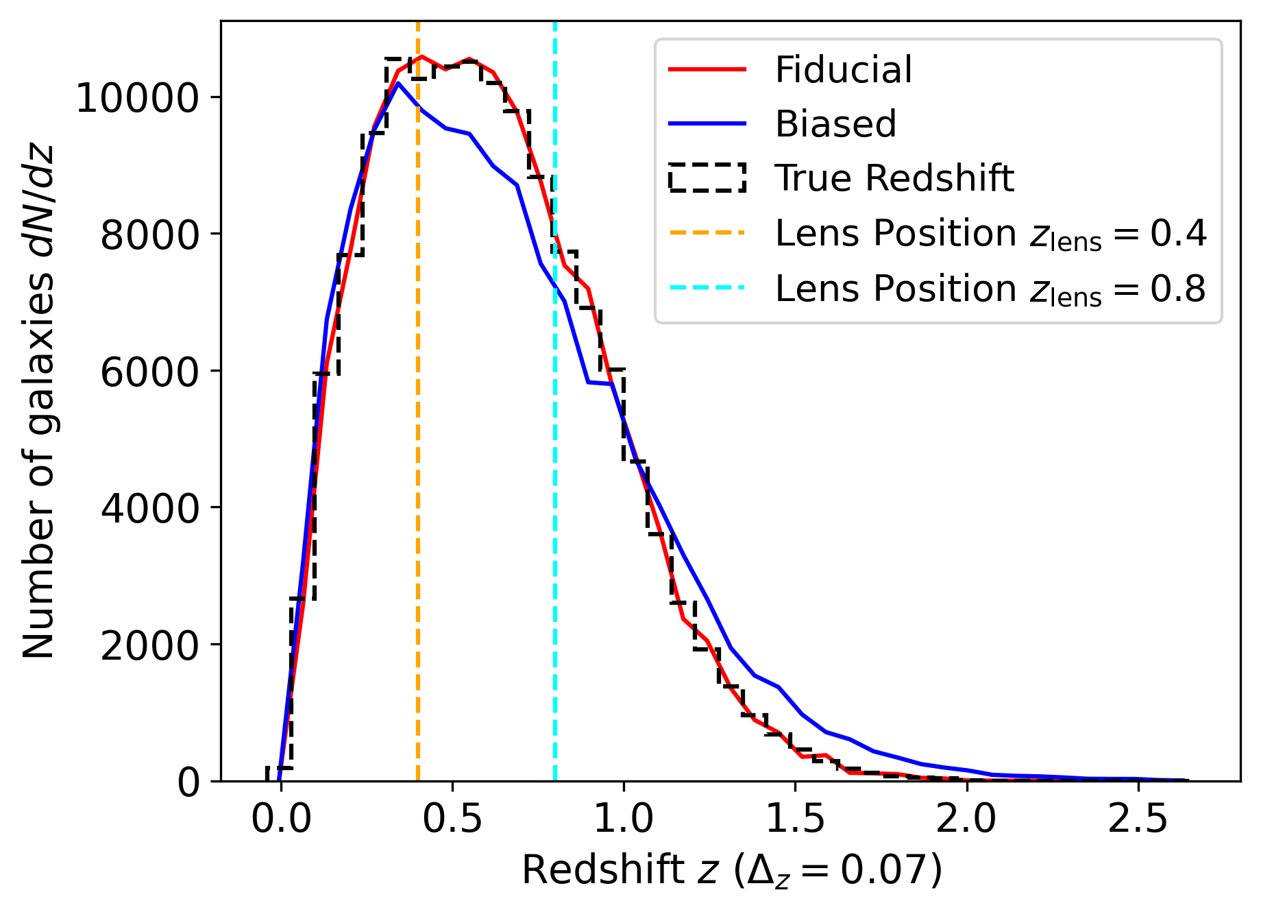
The (red/blue) line show the sample redshift distribution estimates obtained for the (Fiducial/Biased) scenarios as described in the text.
5 Sample Selection optimisation
§ 4 introduced our fast methodology to unfold source sample redshift distributions (sample-pz) and our sample selection methodology that partitions the source sample into included and excluded populations using a mixture model. In the following section we will discuss our methodology to optimise this selection, balancing the tradeoff between removing bins with a high probability of containing galaxies with biased redshifts and keeping a larger source sample for increased constraining power on the inferred cluster mass. We will start the discussion by taking a look at suitable metrics to measure the aforementioned tradeoff.
5.1 Metrics
As discussed in § 2 it is appropriate to quantify photometric redshift error induced systematics in weak lensing cluster mass estimates using distances between a true and estimated . In the following, we make the simplifying assumption that we can estimate this systematic using the photometric redshift calibration techniques described in § 1. This means that we are assuming that we are able to use e.g. spatial cross-correlation redshift estimation techniques to calibrate the sample-pz and we neglect the intrinsic error or the residual systematics in this calibration technique. This will not be perfectly possible in practice, and we will discuss the effect of calibration error on the presented optimisation scheme in § 8.
Since is an integrated quantity we note that an underestimation/overestimation of the integrand as a function of redshift can be compensated by an overestimation/underestimation at a different redshift. A comparable example of this is illustrated in Fig. 19 of Rau et al. (2015) in the context of the lensing efficiency term in cosmic shear power spectra that can “hide” model error due to photometric redshift systematics. Thus, the value of , being a quantity integrated over the sample-pz, might not be globally biased, because of compensating model misspecifications in the integrand. This is still undesirable, because the resulting model misspecification will depend on the lensing geometry, impact inferences of cosmological parameters that enter the integrand and mis-calibrate uncertainty quantification. We, therefore, only consider metrics that are defined in redshift intervals of the source sample and provide summary statistics that are robust against this effect. In the following we denote the corresponding quantities of interest with the subscript (fid/bias) for (fiducial/biased).
The absolute bin-wise distance between biased and fiducial estimates in bin is defined as
| (30) |
where denotes the index set of the (fiducial/biased) histogram bins and
| (31) |
Here, denotes the integrand of Eq. 2 evaluated at the midpoint of the histogram bin and the normalized ‘height’ of sample-pz bin (see Eq. 7). We note that we will only consider sample redshift distribution point estimates, which we define using the mean of the Dirichlet posterior and quantities derived thereof in the following until otherwise stated, i.e. we are not considering posterior uncertainty in the sample redshift inference.
5.2 Combinatorial optimisation
We define the “total gain” as the tradeoff between the “value” of the selection and the summed, or “total cost” of all included redshift bins in terms of their impact on systematic biases in
| (32) |
where is the tradeoff parameter (see below). Using Eq. 30 we define the cost function as:
| (33) |
and the value function as
| (34) |
Here, denotes the number of galaxies in redshift histogram bin and the index set denotes all sample-pz histogram bins with midpoint redshift larger than . Our optimisation objective is to find 111Here, denotes the powerset of . such that is maximized for a selected value of . Maximizing implies finding the maximum sample size that we retain while minimizing the bias in the modelling of . The tradeoff between these terms is governed by the variable.
The problem described in this section resembles a knapsack problem, where we would like to assemble bins such that the residual systematic is below a given threshold while maximizing e.g. the amount of background galaxies kept in the sample, thus increasing the signal-to-noise. However, a naive application of the knapsack optimisation using dynamic programming is not valid because we optimise the construction of a mixture model. In this case, it can be shown by counterexample that dynamic programming, in general, will not find the optimal solution.
5.2.1 Algorithm: Cross-Entropy optimisation
A flexible and easy method to perform combinatorial optimisation that we found to work well in this context is cross entropy optimisation (Rubinstein, 1999; Botev et al., 2013). This probabilistic optimisation scheme starts by defining an initial probability vector of Bernoulli variables with for all .
We then repeat the following steps until convergence:
-
1.
Generate 1000 realisations of the multivariate Bernoulli distribution
-
2.
Evaluate on each generation
-
3.
Select the best 50% realisations with respect to
-
4.
Update , where the sum goes over the number of selected realisations and denotes the indicator function that is unity for each realisation , if and zero otherwise
-
5.
We continue with (i) using the updated .
6 Results
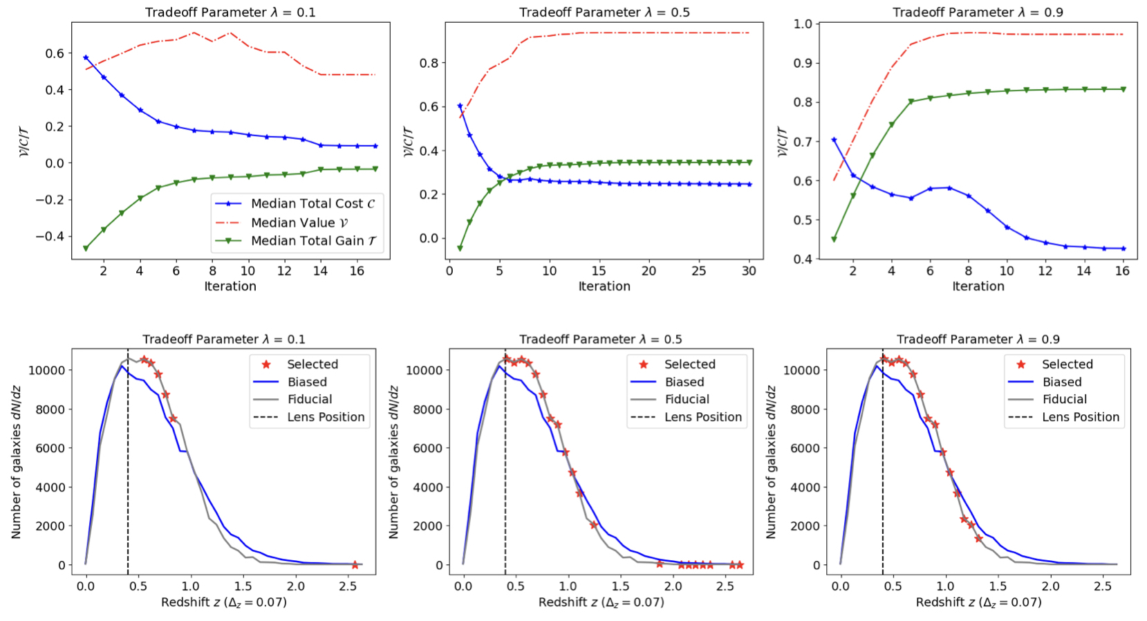
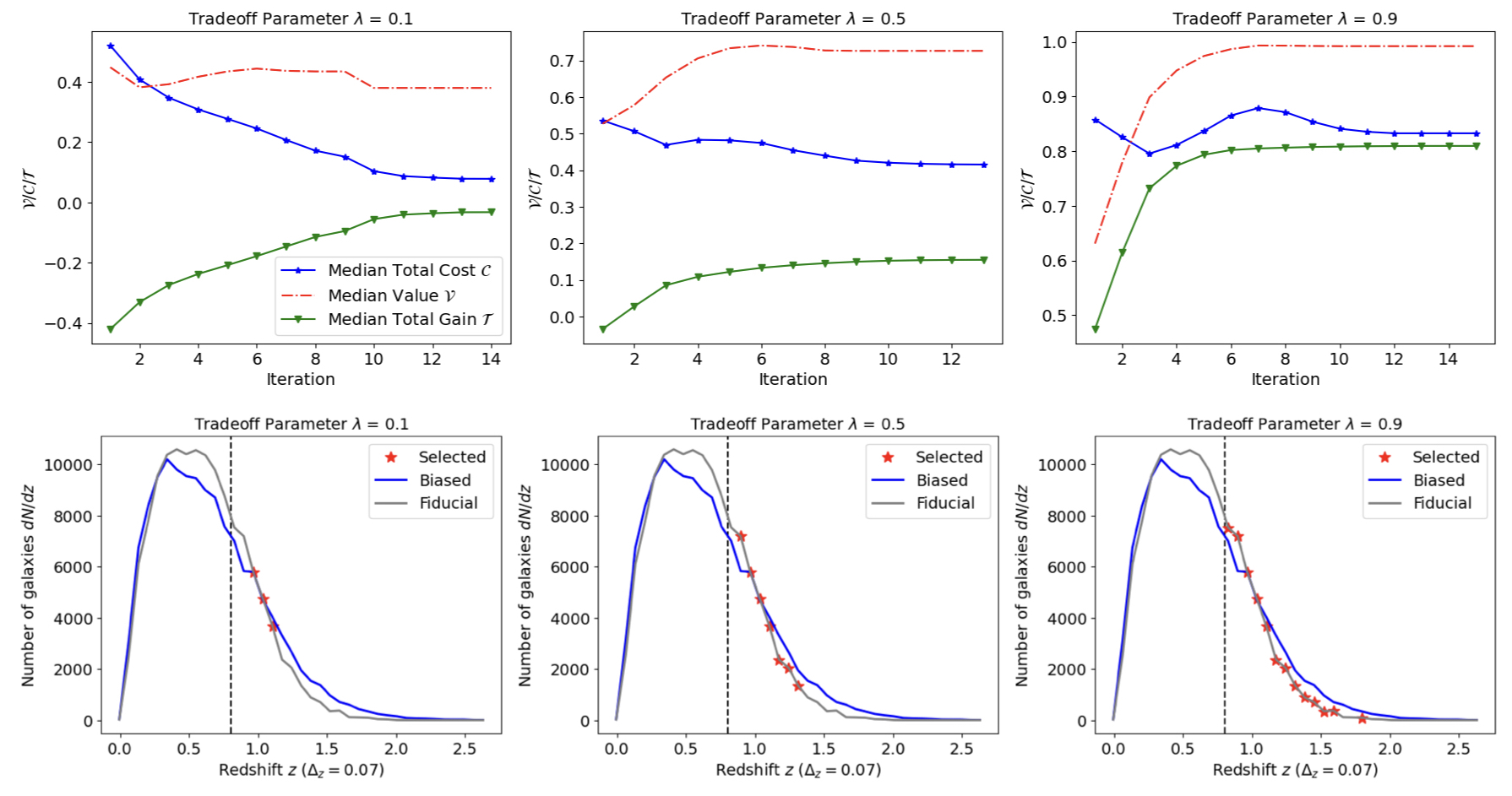
We demonstrate the optimisation (see § 5) using the photometric redshift error model (see § 3) for parameters listed in Tab. 2 and a cluster lens at redshift (see Fig. 2) and (see Fig. 3).
We run the algorithm for 10 iterations of steps (i) - (v) with 1000 realisations of the Bernoulli, cutting at the 0.5 quantile to select the best samples from each set of realisations using the total gain as the optimisation objective.
The upper panels of Fig. 2 and Fig. 3 show the tradeoff between the value and cost, where we show the median cost (blue, stars), value (red, doted-dashed) and total gain (green, triangle) as a function of the cross entropy optimisation iteration. The subpanels correspond to different values of the tradeoff parameter . As expected we see that the total gain is dominated by the cost function for low , converging within 10 iterations. In this case fewer galaxies are retained in the sample. Similarly, higher values of put less weight on the reduction of systematic bias due to photometric redshift error and, therefore, the final sample retains more galaxies. We see in all panels that the scheme converges within less than 30 iterations, often after 10. Since we are using a heuristic combinatorial optimisation scheme, the , and don’t have to monotonially decrease, even though this is true in the vast majority of cases. For , we reduce the critical surface mass density modelling bias, as measured using the metric, on the 60-70% level, while maintaining up to 90% of galaxies. More extreme reductions in bias can be achieved using e.g. , where a reduction of over 90% in the model misspecification can be achieved while still maintaining around of galaxies.
The lower panels of Fig. 2 and Fig. 3 show the (Fiducial/Biased) redshift distributions in (grey/blue). We select a redshift bin size of and indicate the respective cluster lens redshift using the vertical black dashed line. The red points indicate the selected bins after optimisation. The different subpanels show the results for different tradeoff parameters . As discussed in § 5 the algorithm (removes/retains) more bins for (smaller/larger) values of . As a result the selected redshift bins (red stars) are more numerous and extend to higher redshift for larger values of . Note that should not be interpreted as a fraction because it represents a relative weight between a value and total cost function. While the value function in this case is the total number of galaxies in the sample, the relative fraction of galaxies retained after optimisation will not equal .
We identify a bias between fiducial and biased sample redshift distributions at , which is close to the cluster lens for both lens redshifts. Despite this apparent bias, the combinatorial optimisation scheme consistently selects redshift bins in this redshift region. This is because Eq. 2 is an increasing function of redshift, which means that lower redshift bins will contribute less to the overall cost. At the same time, we note that the redshift bins closer to the lens also contain the majority of galaxies in the source sample, which incentivises retaining them. In contrast, we note that the tail distribution is consistently not selected.
We note however, that a more complex modelling, that includes the redshift-dependent signal-to-noise in the tangential shear measurement into the analysis will likely favour a different optimal bin configuration. We leave this investigation for future work. We finally note that computationally the cross-entropy optimisation is quite efficient, where convergence is obtained within 30 seconds on a Macbook Air M2 2022. This low computational cost, coupled with the modelling flexibility supported by this very generic optimisation routine, makes this simple method an ideal choice for the more complex modelling approaches that we want to tackle in the future.
7 Practical Application to Cluster Mass Measurements
In the following, we detail how the described approach to sample selection can be applied to a practical cluster weak-lensing analysis. We discuss the prospective application in 5 steps: defining the optimisation objective and hierarchical population model, fitting the hierarchical population model using the full data, selecting a suitable decomposition in included and excluded populations, running the optimisation, extracting the results and using the optimised galaxy sample in the subsequent analysis.
7.1 Optimisation objective and hierarchical population model
Starting with the analysis, we define a suitable cost and value function. The cross-entropy optimisation algorithm is used here to optimise a total gain function that is constructed from the tradeoff between expected cost and value. Alternatively, if we want the cost of the optimised sample to lie below a certain limit, the cross-entropy optimisation algorithm can also optimise the value function while maintaining a cost below a set threshold. This flexibility allows us to tune the sample optimisation towards specific science goals, such as reducing the systematic error budget below the statistical.
We then define and fit a statistical model to describe the population of galaxies in latent space. In this work, we use variational inference for good performance during combinatorial optimisation. However, other techniques like MCMC methods are also possible.
7.2 Sample Selection
After defining a suitable optimisation objective and fitting a hierarchical population model that describes the distribution of galaxy quantities of interest in latent space, we can define the bins that are included and excluded in the population model. Since we only use the included latent parameters of the population model in the subsequent inference, it effectively removes the influence of galaxies with a high probability of lying within excluded bins from the fit. Thus, if their photometric redshift is incorrect, we can significantly remove biases in the modelling of the critical surface density in this way.
7.3 Running the optimisation
The cross-entropy optimisation scheme discussed in this work provides a flexible and fast approach to optimise the selection of included and excluded bins to optimise the total gain. The cross-entropy algorithm was described in § 5.2.1, where the tuning parameters are the total number of realisations drawn from the multivariate Bernoulli distribution in step (i) and the fraction of realisations removed at each iteration step in (iii). Increasing the number of realisations generated by the multivariate Bernoulli distribution will lead to a smoother convergence and overall better optima at the expense of a higher computational cost. For this work we chose 1000 realisations as a good tradeoff between these considerations. The fraction of removed realisations is related to the total number of realisations. Removing a higher fraction of generated realisations leads to faster convergence at an increased risk of getting stuck in a local minimum. In our case, we chose 50% in step (iii) as a good tradeoff. We note that since we are assuming the usage of spatial cross-correlations to calibrate the sample redshift distribution and will obtain error estimates that enter our cost functions, we need to ensure that the cross-correlation data vector takes these selections into account. Since our selection is in redshift and all common cross-correlation techniques constrain the sample redshift distribution in redshift bins, there are no further steps required for our current setup. However, if the selection would be in other quantities of interest like colour, or parameters like stellar mass or star formation rate, we would need to construct additional cross-correlation measurements for each bin in this latent space. We, therefore, recommend using cross-correlation redshift inference codes similar to The-wizz (Morrison et al., 2017) that support the inclusion of these selection functions without re-evaluating the pair counts.
7.4 Extracting the results
The results of the optimisation include a set of bins of the population distribution that are (included/excluded) from final sample and the corresponding posterior weights that describe the probability that a galaxy is (included/excluded). We use posterior mean point estimates for these quantities derived from the full posterior, which are a direct byproduct of fitting and optimizing our hierarchical population model.
7.5 Using the optimised galaxy sample in the subsequent analysis
The optimised weights and population distributions can then be used in the subsequent analysis as follows. When estimators are constructed on the individual galaxy level, e.g. for measuring tangential shear, the aforementioned weights need to be included in the estimation. The posterior probability that the redshift of galaxy is within the included bins, denoted as , is
| (35) |
where is the parameter vector of the optimised variational distribution as discussed in § 4.1. Here we have used the relation
| (36) |
where we omitted the variables and for simplicity. For theory predictions that use the corresponding population distribution, we can marginalize over the sample-pz uncertainty parametrized by the optimised variational distribution, which in this work was chosen to be a Dirichlet.
8 Summary and Conclusions
The mitigation of systematic errors is an important challenge in modern observational cosmology and many areas of fundamental science. The unprecedented size of cosmological datasets that will be observed by Euclid and the Vera Rubin Observatory implies that the accuracy in the modelling of cosmological and astrophysical effects needs to improve at a similar rate. As is the case in many areas of fundamental science, the inference of parameters of interest can be challenging due to degeneracies induced by the survey design. In large area optical surveys, the limited information available from broad-band photometry can lead to large posterior variances for quantities of interest. Therefore, the parametrization of systematics using complex, many parameter models can lead to a very high-dimensional latent space. This can render inferences computationally expensive and sensitive to prior choices.
This work proposes an alternative to this approach using weak lensing cluster mass estimation as an example. We use the fact that the error in the modelling of is a strong function of redshift and galaxy type and that abating systematic biases for a moderate reduction in sample size is attractive for these analyses. We “remove” histogram bins from the latent space to reduce the photometric redshift error in cluster mass estimates by constructing a mixture model of included/excluded galaxy populations. By optimizing the composition of this mixture model using the cross-entropy method, we are able to reduce the modelling bias in by 60-70%, while maintaining 90% of the source galaxy sample. Of course these numbers will strongly depend on the analysis in question. However, especially in scenarios where modelling error is a strong function of the latent parameters, this approach provides a powerful opportunity to optimise the statistical model.
We note that our method is different from imposing cuts on observed quantities like colours, as we still perform inference on the full data and afterwards optimise our selection in latent space. In future work this will allow the inclusion of confounding variables and extended analyses to test if such ‘interventions’ are really the identifiable cause of a reduction in the systematic.
The latter is not a trivial claim, as discussed in § 2, where modelling errors in the sample redshift distribution can over- and underestimate the integrand at different redshift intervals. This under- and overestimation can compensate and lead to a low estimated modelling error despite large residual systematics. Similar issues can arise upon including confounding variables like e.g. galaxy type into the model. Galaxy type impacts both the model error in (photometry-based) redshift inference as well as galaxy-dark matter bias modelling error. As a result “removing” a given redshift bin might cause a spurious reduction in the bias, if the cross-correlation calibration was also biased for this galaxy population. We finally note that the issues discussed here arise in multiple areas of science and as such the presented method will have applications beyond cluster cosmology like cosmological probes based on 2 point function measurements.
In the advent of large-area photometric surveys like LSST and Euclid, the control of systematics will be vital. Optimizing the sample selection to the science case is critical to control these confounding effects and to facilitate cosmological analyses with well-controlled fidelity.
Acknowledgements
Work at Argonne National Laboratory was supported by the U.S. Department of Energy, Office of High Energy Physics. Argonne, a U.S. Department of Energy Office of Science Laboratory, is operated by UChicago Argonne LLC under contract no. DE-AC02-06CH11357. MMR and NR acknowledges the Laboratory Directed Research and Development (LDRD) funding from Argonne National Laboratory, provided by the Director, Office of Science, of the U.S. Department of Energy under Contract No. DE-AC02-06CH11357. Work at Argonne National Laboratory was also supported under the U.S. Department of Energy contract DE-AC02-06CH11357.
Data Availability
The data and analysis products, as well as the software, will be made publicly available after paper acceptance or earlier upon reasonable request.
References
- Abazajian et al. (2016) Abazajian K. N., et al., 2016, arXiv e-prints, p. arXiv:1610.02743
- Abbott et al. (2020) Abbott T. M. C., et al., 2020, Phys. Rev. D, 102, 023509
- Ade et al. (2019) Ade P., et al., 2019, J. Cosmology Astropart. Phys., 2019, 056
- Alarcon et al. (2020) Alarcon A., Sánchez C., Bernstein G. M., Gaztañaga E., 2020, MNRAS, 498, 2614
- Albrecht et al. (2006) Albrecht A., et al., 2006, arXiv e-prints, pp astro–ph/0609591
- Allen et al. (2011) Allen S. W., Evrard A. E., Mantz A. B., 2011, ARA&A, 49, 409
- Applegate et al. (2014) Applegate D. E., et al., 2014, MNRAS, 439, 48
- Arnouts et al. (1999) Arnouts S., Cristiani S., Moscardini L., Matarrese S., Lucchin F., Fontana A., Giallongo E., 1999, MNRAS, 310, 540
- Bartelmann & Schneider (2001) Bartelmann M., Schneider P., 2001, Phys. Rep., 340, 291
- Bellagamba et al. (2018) Bellagamba F., Roncarelli M., Maturi M., Moscardini L., 2018, MNRAS, 473, 5221
- Benítez (2000) Benítez N., 2000, ApJ, 536, 571
- Benson et al. (2014) Benson B. A., et al., 2014, in Holland W. S., Zmuidzinas J., eds, Society of Photo-Optical Instrumentation Engineers (SPIE) Conference Series Vol. 9153, Millimeter, Submillimeter, and Far-Infrared Detectors and Instrumentation for Astronomy VII. p. 91531P (arXiv:1407.2973), doi:10.1117/12.2057305
- Bleem et al. (2024) Bleem L. E., et al., 2024, The Open Journal of Astrophysics, 7, 13
- Bocquet et al. (2023) Bocquet S., et al., 2023, arXiv e-prints, p. arXiv:2310.12213
- Bocquet et al. (2024) Bocquet S., et al., 2024, arXiv e-prints, p. arXiv:2401.02075
- Böhringer & Schartel (2013) Böhringer H., Schartel N., 2013, Astronomische Nachrichten, 334, 482
- Bonnett (2015) Bonnett C., 2015, MNRAS, 449, 1043
- Botev et al. (2013) Botev Z. I., Kroese D. P., Rubinstein R. Y., L’Ecuyer P., 2013, in Rao C., Govindaraju V., eds, Handbook of Statistics, Vol. 31, Handbook of Statistics. Elsevier, pp 35–59, doi:https://doi.org/10.1016/B978-0-444-53859-8.00003-5, https://www.sciencedirect.com/science/article/pii/B9780444538598000035
- Buchs et al. (2019) Buchs R., et al., 2019, Monthly Notices of the Royal Astronomical Society, 489, 820
- Bulbul et al. (2024) Bulbul E., et al., 2024, arXiv e-prints, p. arXiv:2402.08452
- Carrasco Kind & Brunner (2013) Carrasco Kind M., Brunner R. J., 2013, MNRAS, 432, 1483
- Cataneo & Rapetti (2018) Cataneo M., Rapetti D., 2018, International Journal of Modern Physics D, 27, 1848006
- Cawthon et al. (2022) Cawthon R., et al., 2022, MNRAS, 513, 5517
- Clerc et al. (2024) Clerc N., et al., 2024, arXiv e-prints, p. arXiv:2402.08457
- Collister & Lahav (2004) Collister A. A., Lahav O., 2004, Publications of the Astronomical Society of the Pacific, 116, 345
- Conroy (2013) Conroy C., 2013, ARA&A, 51, 393
- Costanzi et al. (2019) Costanzi M., et al., 2019, MNRAS, 482, 490
- Davis et al. (2017) Davis C., et al., 2017, arXiv e-prints, p. arXiv:1710.02517
- Euclid Collaboration et al. (2019) Euclid Collaboration et al., 2019, A&A, 627, A23
- Feldmann et al. (2006) Feldmann R., et al., 2006, MNRAS, 372, 565
- Gatti et al. (2018) Gatti M., et al., 2018, MNRAS, 477, 1664
- Gatti et al. (2022) Gatti M., et al., 2022, MNRAS, 510, 1223
- Geiger & Heckerman (1970) Geiger D., Heckerman D., 1970, Annals of Statistics, 25
- Gerdes et al. (2010) Gerdes D. W., Sypniewski A. J., McKay T. A., Hao J., Weis M. R., Wechsler R. H., Busha M. T., 2010, ApJ, 715, 823
- Ghirardini et al. (2024) Ghirardini V., et al., 2024, arXiv e-prints, p. arXiv:2402.08458
- Giannini et al. (2024) Giannini G., et al., 2024, MNRAS, 527, 2010
- Grandis et al. (2021) Grandis S., Bocquet S., Mohr J. J., Klein M., Dolag K., 2021, MNRAS, 507, 5671
- Greisel et al. (2015) Greisel N., Seitz S., Drory N., Bender R., Saglia R. P., Snigula J., 2015, MNRAS, 451, 1848
- Hartley et al. (2020) Hartley W. G., et al., 2020, MNRAS, 496, 4769
- Hildebrandt et al. (2021) Hildebrandt H., et al., 2021, A&A, 647, A124
- Hilton et al. (2021) Hilton M., et al., 2021, ApJS, 253, 3
- Hoyle (2016) Hoyle B., 2016, Astronomy and Computing, 16, 34
- Huterer et al. (2014) Huterer D., Lin H., Busha M. T., Wechsler R. H., Cunha C. E., 2014, MNRAS, 444, 129
- Ilbert et al. (2006) Ilbert O., et al., 2006, A&A, 457, 841
- Kullback & Leibler (1951) Kullback S., Leibler R. A., 1951, The annals of mathematical statistics, 22, 79
- LSST Science Collaboration et al. (2009) LSST Science Collaboration et al., 2009, arXiv e-prints, p. arXiv:0912.0201
- Leistedt et al. (2016) Leistedt B., Mortlock D. J., Peiris H. V., 2016, MNRAS, 460, 4258
- Lesci et al. (2022a) Lesci G. F., et al., 2022a, A&A, 659, A88
- Lesci et al. (2022b) Lesci G. F., et al., 2022b, A&A, 659, A88
- Malz & Hogg (2020) Malz A. I., Hogg D. W., 2020, arXiv e-prints, p. arXiv:2007.12178
- Masters et al. (2017) Masters D. C., Stern D. K., Cohen J. G., Capak P. L., Rhodes J. D., Castander F. J., Paltani S., 2017, ApJ, 841, 111
- Masters et al. (2019) Masters D. C., et al., 2019, ApJ, 877, 81
- McQuinn & White (2013) McQuinn M., White M., 2013, MNRAS, 433, 2857
- Ménard et al. (2013) Ménard B., Scranton R., Schmidt S., Morrison C., Jeong D., Budavari T., Rahman M., 2013, arXiv e-prints, p. arXiv:1303.4722
- Morrison et al. (2017) Morrison C. B., Hildebrandt H., Schmidt S. J., Baldry I. K., Bilicki M., Choi A., Erben T., Schneider P., 2017, MNRAS, 467, 3576
- Mroczkowski et al. (2019) Mroczkowski T., et al., 2019, Space Sci. Rev., 215, 17
- Myles et al. (2021) Myles J., et al., 2021, MNRAS, 505, 4249
- Newman (2008) Newman J. A., 2008, ApJ, 684, 88
- Newman & Gruen (2022) Newman J. A., Gruen D., 2022, ARA&A, 60, 363
- Newman et al. (2015) Newman J. A., et al., 2015, Astroparticle Physics, 63, 81
- Oke (1974) Oke J. B., 1974, ApJS, 27, 21
- Planck Collaboration et al. (2016) Planck Collaboration et al., 2016, A&A, 594, A24
- Pratt et al. (2019) Pratt G. W., Arnaud M., Biviano A., Eckert D., Ettori S., Nagai D., Okabe N., Reiprich T. H., 2019, Space Sci. Rev., 215, 25
- Raccanelli et al. (2017) Raccanelli A., Rahman M., Kovetz E. D., 2017, MNRAS, 468, 3650
- Rau et al. (2015) Rau M. M., Seitz S., Brimioulle F., Frank E., Friedrich O., Gruen D., Hoyle B., 2015, MNRAS, 452, 3710
- Rau et al. (2020) Rau M. M., Wilson S., Mandelbaum R., 2020, MNRAS, 491, 4768
- Rau et al. (2023) Rau M. M., et al., 2023, MNRAS, 524, 5109
- Rubinstein (1999) Rubinstein R., 1999, Methodology And Computing In Applied Probability, 1, 127
- Rykoff et al. (2014) Rykoff E. S., et al., 2014, ApJ, 785, 104
- Rykoff et al. (2016) Rykoff E. S., et al., 2016, ApJS, 224, 1
- Salvati et al. (2022) Salvati L., et al., 2022, ApJ, 934, 129
- Salvato et al. (2019) Salvato M., Ilbert O., Hoyle B., 2019, Nature Astronomy, 3, 212
- Sánchez & Bernstein (2019) Sánchez C., Bernstein G. M., 2019, MNRAS, 483, 2801
- Scottez et al. (2016) Scottez V., et al., 2016, MNRAS, 462, 1683
- Sommer et al. (2022) Sommer M. W., Schrabback T., Applegate D. E., Hilbert S., Ansarinejad B., Floyd B., Grandis S., 2022, MNRAS, 509, 1127
- Sunyaev & Zel’dovich (1972) Sunyaev R. A., Zel’dovich Y. B., 1972, Comments on Astrophysics and Space Physics, 4, 173
- Tagliaferri et al. (2003) Tagliaferri R., Longo G., Andreon S., Capozziello S., Donalek C., Giordano G., 2003, Neural Networks for Photometric Redshifts Evaluation. pp 226–234, doi:10.1007/978-3-540-45216-4_26
- The LSST Dark Energy Science Collaboration et al. (2018) The LSST Dark Energy Science Collaboration et al., 2018, arXiv e-prints, p. arXiv:1809.01669
- Umetsu (2020) Umetsu K., 2020, A&ARv, 28, 7
- Voit (2005) Voit G. M., 2005, Reviews of Modern Physics, 77, 207
- van den Busch et al. (2020) van den Busch J. L., et al., 2020, A&A, 642, A200