Mitigating the binary viewing angle bias for standard sirens

Abstract

The inconsistency between experiments in the measurements of the local Universe expansion rate, the Hubble constant, suggests unknown systematics in the existing experiments or new physics. Gravitational-wave standard sirens, a method to independently provide direct measurements of the Hubble constant, have the potential to address this tension. Before that, it is critical to ensure there is no substantial systematics in the standard siren method. A significant systematic has been identified when the viewing angle of the gravitational-wave sources, the compact binary coalescences, is inferred inaccurately from electromagnetic observations of the sources. Such systematic has led to more than 10% discrepancy in the standard siren Hubble constant measurements with the observations of binary neutron star merger, GW170817. In this Letter, we develop a new formalism to infer and mitigate this systematic. We demonstrate that the systematic uncertainty of the Hubble constant measurements can be reduced to smaller than their statistical uncertainty with 5, 10, and 20 binary neutron star merger observations. We show that our formalism successfully reduces the systematics even if the shape of the biased viewing angle distribution does not follow precisely the model we choose. Our formalism ensures unbiased standard siren Hubble constant measurements when the binary viewing angles are inferred from electromagnetic observations.

Introduction.– The expansion rate of the local Universe, the Hubble constant ($H_{0}$), is one of the most important constants in modern cosmology. Despite numerous observational efforts, a statistically significant discrepancy persists between direct measurements and indirect inferences of $H_{0}$ Kamionkowski and Riess (2022); Aghanim et al. (2020); Alam et al. (2017); Riess et al. (2016, 2022); Ross et al. (2015); Di Valentino et al. (2021); Verde et al. (2019). For example, the tension between the Hubble constant measured by SH0ES team using Type Ia supernovae and inferred by Planck collaboration using cosmic microwave background is as large as $\sim 8\%$ Aghanim et al. (2020); Riess et al. (2022).

Gravitational wave (GW) observations of compact binary coalescences (CBCs) offer an independent and direct measurement of $H_{0}$. The luminosity distance to CBCs can be inferred from the amplitude of the GW signals. When combining with the redshift estimates, we can measure the cosmological parameters Schutz (1986). This is known as the ‘standard siren’ method. The proximity of CBCs detected by the current generation of GW detectors, LIGO, Virgo, and KAGRA Abbott et al. (2020a); Aasi et al. (2015); Acernese et al. (2014); Abbott et al. (2018); Akutsu et al. (2020), makes them ideal for the measurement of the Hubble constant. There are several possibilities to estimate the redshift of CBCs. If an electromagnetic (EM) counterpart of a CBC is observed, it is possible to precisely localize the CBC’s host galaxy, and determine the redshift from spectral follow-up or existing galaxy catalogs Schutz (1986); Holz and Hughes (2005). With about 50 CBCs and their EM counterparts, $H_{0}$ can be determined to $\sim 2\%$ precision, shedding light on the Hubble tension Schutz (1986); Chen et al. (2018); Nissanke et al. (2013); Feeney et al. (2019).

Furthermore, it is known that the precision of standard siren measurements can be improved by constraining CBC’s viewing angle ($\iota$)Chen et al. (2019); Margutti et al. (2017); Wu and MacFadyen (2018); Mooley et al. (2018); Evans et al. (2017); Finstad et al. (2018). GW emissions from a CBC are anisotropic. The emissions are stronger along the rotational axis of binaries. Therefore, signals received from a faraway face-on binary are similar to those from a nearby edge-on binary Abbott et al. (2019). By constraining the viewing angle, the degeneracy between binary distance and viewing angle can be broken, tightening the estimate of luminosity distance, and reducing the uncertainty of $H_{0}$ measurements Chen et al. (2019). Nicely, the observations of EM counterparts not only provide the redshift estimate but also allow for the measurement of CBC’s viewing angle. The observations of the jet and afterglow of gamma-ray burst and kilonova following the binary neutron star (BNS) merger, GW170817Abbott et al. (2017a, b), have been used to constrain the binary’s viewing angle Mooley et al. (2018); Evans et al. (2017); Finstad et al. (2018); Peng et al. (2024) and improve the standard siren $H_{0}$ measurements Guidorzi et al. (2017); Hotokezaka et al. (2018); Dhawan et al. (2020); Palmese et al. (2023). In Fig. 1, we give an example of the standard siren $H_{0}$ measurement by combining three simulated BNS observations with (orange) and without (blue) viewing angle constraints. The $H_{0}$ measurement uncertainty with viewing angle constraints is substantially smaller.

However, these constraints on viewing angle are EM model-dependent and subject to incoherent existing analyses. Biased viewing angle constraints can lead to significant bias in $H_{0}$ Chen (2020). For example, the estimate of the viewing angle of GW170817 varied from $22^{\circ}$ to $50^{\circ}$ Guidorzi et al. (2017); Mooley et al. (2018); Hotokezaka et al. (2018); Dhawan et al. (2020); Wang and Giannios (2021); Finstad et al. (2018); Heinzel et al. (2021); Palmese et al. (2023), leading to $H_{0}$ measurements differed by more than 10% (e.g., $H_{0}=68.3^{+4.6}_{-4.5}$ km/s/Mpc by Mooley et al. (2018) and $H_{0}=75.5^{+11.6}_{-9.6}$ km/s/Mpc by Guidorzi et al. (2017)). This is a discrepancy larger than the difference between other $H_{0}$ measurements, making it impossible to resolve the tension.

Figure 1: An example of standard siren $H_{0}$ posterior by combining three simulated 1.4-1.4$M_{\odot}$ binary neutron star mergers detected by LIGO-Virgo. The blue curve assumes no extra information about the binary viewing angle. The orange curve assumes the viewing angles are constrained accurately with $1\sigma$ uncertainty of $5^{\circ}$, and the gray curve assumes the viewing angles are overestimated by $20^{\circ}$ (with $1\sigma$ statistical uncertainty of $5^{\circ}$). The vertical dashed line indicates the $H_{0}$ value chosen for the simulations.

In Fig. 1, we give an example of the $H_{0}$ measurement assuming $20^{\circ}$ overestimate of the viewing angle (gray), showing the impact of the bias. The impact is expected to become more significant as the number of observations increases (see also Fig. 3 for the impact when there are 10 BNS observations).

In this Letter, we develop a new method to mitigate this bias by using the viewing angle estimated from GW signals. Although the viewing angles are often poorly constrained in GWs Chen et al. (2019), the measurements are well-established and are expected to be unbiased Abbott et al. (2019). Therefore, we can use the GW-inferred viewing angles from multiple observations to reveal the bias in EM observations. In the following, we first lay out our formalism. We then simulate BNSs detected by LIGO and Virgo, and assume the binary viewing angles are measured inaccurately from EM observations with four different types of bias. We use these simulations to show how the biases affect the standard siren $H_{0}$ measurements. Finally, we demonstrate that our formalism successfully reduces the systematics to less than the statistical uncertainty of the $H_{0}$ measurements.

Mitigating the binary viewing angle bias.– Although GW detectors are able to measure the binary inclination angle, $\theta_{\rm JN}$, which carries the directional information of the binary rotation (clockwise or counterclockwise), most EM observations only infer the binary viewing angle, $\iota$, which is defined as $\iota\equiv{\rm min}(\theta_{\rm JN},180^{\circ}-\theta_{\rm JN})$.

For a binary with viewing angle $\iota_{*}$, we assume the EM data suggests the viewing angle to be $\iota_{*}+b$, where $b$ is the amount of bias. The bias is not necessarily the same for different BNS events. Suppose the biases among different events follow an unknown underlying probability density distribution, we parametrize this distribution with a vector of parameters, $\vec{\beta}$. Following this parameterization, we jointly infer $H_{0}$ and $\vec{\beta}$ using Bayesian inference, and write the posterior of $(H_{0},\vec{\beta})$ as

$$p(H_{0},\vec{\beta}|\vec{\mathcal{D}})=\pi(H_{0},\vec{\beta})\frac{\mathcal{L}(\vec{\mathcal{D}}|H_{0},\vec{\beta})}{p(\vec{\mathcal{D}})},$$ (1)

where $\pi(H_{0},\vec{\beta})$ stands for the prior on $(H_{0},\vec{\beta})$. $\mathcal{L}(\vec{\mathcal{D}}|H_{0},\vec{\beta})$ is the likelihood function, and $p(\vec{\mathcal{D}})$ is the evidence. $\vec{\mathcal{D}}\equiv({\vec{\mathcal{D}}_{\rm GW}},\vec{\mathcal{D}}_{\rm EM})$ denotes the data from GW and EM observations. When there are $N$ BNS events, $\vec{\mathcal{D}}$ represents the collection of data $\vec{\mathcal{D}}=(\vec{\mathcal{D}}_{\rm GW}^{1},\vec{\mathcal{D}}^{1}_{\rm EM},\vec{\mathcal{D}}_{\rm GW}^{2},\vec{\mathcal{D}}^{2}_{\rm EM},...,\vec{\mathcal{D}}_{\rm GW}^{N},\vec{\mathcal{D}}^{N}_{\rm EM})$. Assuming each BNS observation is independent, we can rewrite Eq. 1 as

$$p(H_{0},\vec{\beta}|\vec{\mathcal{D}})\propto\pi(H_{0},\vec{\beta})\prod_{i=1}^{N}\mathcal{L}(\vec{\mathcal{D}}_{\rm GW}^{i},\vec{\mathcal{D}}^{i}_{\rm EM}|H_{0},\vec{\beta}).$$ (2)

If we use $\vec{\Theta}$ to denote the collection of binary physical parameters, such as luminosity distance $D_{L}$, redshift $z$, inclination angle $\theta_{\rm JN}$, mass, and spin, we can write the likelihood of $i$th event as

$$\begin{split}&\mathcal{L}(\vec{\mathcal{D}}_{\rm GW}^{i},\vec{\mathcal{D}}^{i}_{\rm EM}|H_{0},\vec{\beta})=\\ &\frac{\int\mathcal{L}(\vec{\mathcal{D}}_{\rm GW}^{i},\vec{\mathcal{D}}^{i}_{\rm EM},\vec{\Theta}|H_{0},\vec{\beta})d\vec{\Theta}}{\int\displaylimits_{\begin{subarray}{c}\vec{\mathcal{D}}_{\rm GW}>\vec{\mathcal{D}}_{\rm GW,th}\\ \vec{\mathcal{D}}_{\rm EM}>\vec{\mathcal{D}}_{\rm EM,th}\end{subarray}}\mathcal{L}(\vec{\mathcal{D}}_{\rm GW},\vec{\mathcal{D}}_{\rm EM},\vec{\Theta}|H_{0},\vec{\beta})d\vec{\Theta}d\vec{\mathcal{D}}_{\rm GW}d\vec{\mathcal{D}}_{\rm EM}},\end{split}$$ (3)

where $\vec{\mathcal{D}}_{\rm GW,th}$ and $\vec{\mathcal{D}}_{\rm EM,th}$ denote the detection threshold of GW detectors and EM telescopes. The denominator of Eq. 3 accounts for the selection effect Thrane and Talbot (2019); Mandel et al. (2019); Vitale et al. (2020), since not all sources are equally detectable. Sources with certain physical parameters are easier to detect, introducing a selection bias when combining multiple events for Bayesian inference. To correct for the selection effects, we account for how probable it is to detect a source with a particular set of parameters.

We can further separate $\vec{\Theta}$ into relevant physical parameters ($D_{L}$,$z$,$\Theta_{\rm JN}$) and other physical parameters $\vec{\Theta}^{{}^{\prime}}$ ( $\vec{\Theta}\supset\{D_{L},z,\Theta_{\rm JN},\vec{\Theta}^{{}^{\prime}}\}$), and write the likelihood for individual event as

$$\begin{split}\mathcal{L}(\vec{\mathcal{D}}_{\rm GW}^{i},\vec{\mathcal{D}}_{\rm EM}^{i}|&H_{0},\vec{\beta})\propto\int d\theta_{\rm JN}dD_{\rm L}dzd\vec{\Theta}^{{}^{\prime}}db\\ &\times p(\vec{\mathcal{D}}_{\rm GW}^{i},\vec{\mathcal{D}}_{\rm EM}^{i},\theta_{\rm JN},D_{\rm L},z,\vec{\Theta}^{{}^{\prime}},b|H_{0},\vec{\beta}).\end{split}$$ (4)

Note that in Eq. 4 we explicitly write the bias $b$ as one of the parameters that affect the data.

Since the GW and EM observations are independent, we can apply the product rules for joint probabilities [$p(A,B|I)=p(A|B,I)p(B|I)$] and write the integrand of Eq. 4 as (see Supplemental Material for step-by-step derivations)

$$\begin{split}&p(\vec{\mathcal{D}}_{\rm GW}^{i},\vec{\mathcal{D}}_{\rm EM}^{i},\theta_{\rm JN},D_{\rm L},z,\vec{\Theta}^{{}^{\prime}},b|H_{0},\vec{\beta})\\ &=\>\mathcal{L}(\vec{\mathcal{D}}_{\rm GW}^{i}|\theta_{\rm JN},D_{\rm L},\vec{\Theta}^{{}^{\prime}})\times\mathcal{L}(\vec{\mathcal{D}}_{\rm EM}^{i}|\theta_{\rm JN},z,\vec{\Theta}^{{}^{\prime}},b)\\ &\times p(\theta_{\rm JN},D_{\rm L},z,\vec{\Theta}^{{}^{\prime}},b|H_{0},\vec{\beta}).\end{split}$$ (5)

Note that the GW and EM data provide the measurements of luminosity distance $D_{L}$ and redshift $z$, respectively, and only the EM data are affected by the viewing angle bias $b$.

Finally, the last term in Eq. 5 can be written as

$$\begin{split}p(\theta_{\rm JN},D_{\rm L},z,\vec{\Theta}^{{}^{\prime}},b|H_{0},\vec{\beta})=&\delta[D_{\rm L}-\hat{D}_{\rm L}(z,H_{0})]\\ &\times p(\theta_{\rm JN})p(z|H_{0})p(\vec{\Theta}^{{}^{\prime}})p(b|\vec{\beta}),\end{split}$$ (6)

where $\delta[D_{\rm L}-\hat{D}_{\rm L}(z,H_{0})]$ is a Dirac $\delta$-function originating from the dependency between luminosity distance, redshift, and $H_{0}$ when other cosmological parameters are fixed, an assumption that is valid for nearby events but can be naturally relaxed when events at higher redshifts are included. $p(\theta_{\rm JN})=\sin{\theta_{JN}}$ since binary inclination angles in the Universe are isotropically distributed. We also assume the sources are uniformly distributed in comoving volume $V_{c}$, another assumption that can be relaxed for high-redshift events. We take $p(z|H_{0})=\frac{dV_{c}(H_{0})}{dz}\frac{1}{1+z}$.

$p(b|\vec{\beta})$ in Eq. 6 represents the probability distribution of the viewing angle bias under a given model. In this Letter, we start with a Normal distribution as our baseline model for $p(b|\vec{\beta})$. We will show later that this baseline model works well to mitigate the bias even if the bias does not follow a Normal distribution. Under this model, the probability distribution is described by two parameters, $\vec{\beta}=(\beta_{1},\beta_{2})$, where $\beta_{1}$ and $\beta_{2}$ represent the mean and standard deviation of the Normal distribution, respectively.

Application to simulated observations.– We simulate 1000 1.4-1.4 M_⊙ BNS detections detected by LIGO-Hanford, LIGO-Livingston, and Virgo with their 4th observing run sensitivities ( aligo_O4high.txt, avirgo_O4high_NEW.txt in Abbott et al. (2020b)) Abbott et al. (2018); Aasi et al. (2015); Acernese et al. (2014) in a Universe following Planck 2015 cosmology DES and Collaborations (2023) ($\Omega_{m}=0.306$, $\Omega_{\Lambda}=0.694$, $\Omega_{k}=0.0$, $H_{0}=67.8$km/s/Mpc). The GW detection threshold is set at a network signal-to-noise ratio of 12 Abbott et al. (2020a); Chen et al. (2021). The BNSs have random inclination and orientation angles, and are distributed uniformly in comoving volume.

We follow the method developed in Chen et al. (2019) to construct the GW likelihood function, $\mathcal{L}(\vec{\mathcal{D}}_{\rm GW}^{i}|\theta_{\rm JN},D_{\rm L},\vec{\Theta}^{{}^{\prime}})$ in Eq. 5. For the EM likelihood, $\mathcal{L}(\vec{\mathcal{D}}_{\rm EM}^{i}|\theta_{\rm JN},z,\vec{\Theta}^{{}^{\prime}},b)$, we assume that the redshift measurements from EM observations have negligible uncertainty, an appropriate assumption when compared to the uncertainty in GW distance measurements Abbott et al. (2017a). For the viewing angle measured in EM observations, we add $\epsilon_{*}$ to each binary viewing angle $\iota_{*}$, where $\epsilon_{*}$ is randomly drawn from a zero-mean Normal distribution with a standard deviation of $5^{\circ}$, to account for the statistical uncertainty of the measurements Margutti et al. (2017); Wu and MacFadyen (2018); Mooley et al. (2018); Evans et al. (2017); Finstad et al. (2018). In addition, we randomly draw a bias $b_{*}$ for each binary from one of the probability distributions described below. Therefore, the likelihood of the viewing angle measured from EM observations is simulated as a 1-dimensional Gaussian function with a $1\sigma$ width of $5^{\circ}$ centering at $\tilde{\iota}=\iota_{*}+\epsilon_{*}+b_{*}$.

To simulate the bias in viewing angle, we explore four potential probability distributions (see examples in Fig. 2): (i) Normal distribution with mean $\gamma_{1}$ and standard deviation $\gamma_{2}$. This is the same type of distribution as our baseline model for $p(b|\vec{\beta})$ in Eq. 6. We pick $\gamma_{1}=[\pm 5^{\circ},\pm 10^{\circ},\pm 20^{\circ}$], and $\gamma_{2}=5^{\circ}$. (ii) Uniform distribution, with supports $[-40^{\circ},0^{\circ}]$, $[-20^{\circ},0^{\circ}]$, $[-10^{\circ},0^{\circ}]$, $[0^{\circ},10^{\circ}]$, $[0^{\circ},20^{\circ}]$, and $[0^{\circ},40^{\circ}]$. (iii) Poisson distribution:

$$p(b_{*})=\begin{cases}\frac{\lambda^{b_{*}}e^{-\lambda}}{b_{*}!}\quad\mbox{if}\quad b_{*}\geq 0\\ \frac{\lambda^{-b_{*}}e^{-\lambda}}{(-b_{*})!}\quad\mbox{if}\quad b_{*}<0\end{cases}$$ (7)

with expected rate parameter $\lambda=10^{\circ},20^{\circ},30^{\circ}$. (iv) Exponential distribution:

$$p(b_{*})=\begin{cases}\frac{1}{\lambda}e^{-\frac{b_{*}}{\lambda}}\quad\mbox{if}\quad b_{*}\geq 0\\ \frac{1}{\lambda}e^{\frac{b_{*}}{\lambda}}\quad\mbox{if}\quad b_{*}<0\end{cases}$$ (8)

with scale parameter $\lambda=10^{\circ},20^{\circ},30^{\circ}$.

Figure 2: Probability density distribution of the bias in viewing angle we study in this Letter. The bias for each simulated BNS event is randomly drawn from these distributions.

We use uniform priors $[20,200]\mbox{km/s/Mpc}$, $[-90^{\circ},90^{\circ}]$, and $[2^{\circ},92^{\circ}-|\beta_{1}|]$ for $H_{0}$, $\beta_{1}$, and $\beta_{2}$ in Eq. 1 respectively. The minimum for $\beta_{2}$ is chosen to avoid numerical effects in the Markov Chain Monte Carlo inference, and the maximum is set by the range of viewing angle $[0^{\circ},90^{\circ}]$.

We randomly select 5, 10, and 20 events out of the 1000 BNS detections and use emcee Foreman-Mackey et al. (2013) to sample the posteriors in Eq. 1. We repeat this process 30 times for all types of bias, and report the average of posteriors in the next section.

Result.– We start with the bias distribution that follows a Normal distribution.

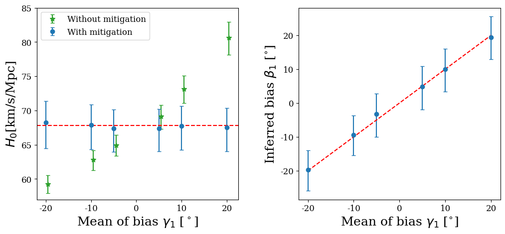
Figure 3: Measurements from 10 simulated BNS detections, averaged over 30 realizations. The horizontal axes label the mean ($\gamma_{1}$) of the viewing angle bias distribution. Here we assume the bias follows a Normal distribution centering at $\gamma_{1}$ with a standard deviation of $5^{\circ}$. Left: The median and symmetric 68% credible interval of the $H_{0}$ posteriors with (blue) and without (green) applying our mitigation formalism. The red dashed line marks the simulated value of $H_{0}$. Right: The median and symmetric 68% credible interval of the inferred bias ($\beta_{1}$) posteriors. The red dashed line represents the line of accurate measurement.

This is the same type of distribution as our parametrized model $p(b|\vec{\beta})$ in Eq. 6. In the left panel of Fig. 3, we present the median and symmetric 68% credible interval of the $H_{0}$ posteriors when combining 10 BNS detections for simulated bias centering at different $\gamma_{1}$. As shown in the figure, the $H_{0}$ measurements significantly deviate from the simulated value even with a small $\gamma_{1}$ when the bias is not mitigated (green). We then show the $H_{0}$ posteriors following our mitigation formalism in blue (Eq. 1 marginalized over $\vec{\beta}$). We find that our formalism successfully reduces the bias in $H_{0}$ to less than their statistical uncertainties for all $\gamma_{1}$.

In the right panel of Fig. 3, we show the $\beta_{1}$ posteriors marginalized over $H_{0}$ and $\beta_{2}$ for simulated bias centering at different $\gamma_{1}$. We find that our formalism can reveal the simulated bias accurately.

In addition to $\sigma=5^{\circ}$ and $\gamma_{2}=5^{\circ}$, we also explore larger $\sigma$ and $\gamma_{2}$. Furthermore, we repeated the simulations for 5 and 20 BNS detections. We find similar results with $H_{0}$ and $\gamma_{1}$ measured accurately.

In reality, the viewing angle bias distribution does not necessarily follow the parameterized model we pick. Therefore, we consider three additional types of bias distributions (Fig. 2) and explore if a Normal distribution is sufficient to mitigate the bias. In Fig. 4, we present the median and symmetric 68% credible interval of the $H_{0}$ posteriors with (blue) and without (green) applying our mitigation formalism for these three types of bias. Even if the bias distribution does not follow a Normal distribution, we can effectively reduce the bias in $H_{0}$ to below the measurement statistical uncertainties when modeling the bias as a Normal distribution. This is because the central limit theorem ensures the mean of the drawn biases $b_{*}$ follows a Normal distribution, which can be successfully captured by our baseline model.

(a)

(b)

(c)

Figure 4: The median and symmetric 68% credible interval of the $H_{0}$ posteriors with (blue) and without (green) applying our mitigation formalism. We assume the viewing angle bias follows a Uniform (top), Poisson (middle), and Exponential (bottom) distribution (see texts for the choices of distribution parameters). These distributions are different from the parameterized model we pick for the bias. The results are measurements from 10 simulated BNS detections, averaged over 30 realizations.

Discussion.– In this Letter, we present a new bright siren inference formalism that successfully mitigates the systematic uncertainty introduced by inaccurate binary viewing angle estimates. Our formalism ensures that the systematic uncertainty lies below the statistical uncertainty of the $H_{0}$ measurements when the binary viewing angle inferred from non-GW channels, such as EM observations, is biased. We show that the bias can be mitigated even if the distribution of the systematics does not precisely follow the model we assume.

The complexity of EM emission modelings, the differences among analyses, and the variations of observing conditions could all lead to bias in the estimate of binary viewing angle. The sources of the bias can be difficult to disentangle, and the characteristics of the bias vary with the choice of data. It is therefore pivotal to demonstrate that our formalism effectively mitigates different types of bias distribution with the chosen baseline model, so that the formalism can be applied in wide-ranging circumstances.

In Figs. 3 and  4, we present the results for 10 simulated BNS detections. We also explore the five-detection scenario and find that five events are already informative enough to reveal and alleviate the bias with our formalism. In addition, we perform the 20-detection simulations to investigate if there is any remaining systematic after applying our formalism. The increased number of events reduces the statistical uncertainty of the measurements and the systematic uncertainty stands out. We do not find any remaining bias.

Our method can be improved if additional knowledge about the distribution of bias is available. For example, we use a Normal distribution to model the probability distribution of the bias in viewing angle in this work. If the shape of the bias distribution is better understood, more accurate models can be used to replace the Normal distribution we adopt. Even if the shape of the bias distribution is unknown, knowledge of the possible range of the bias can be used as the prior $\pi(H_{0},\vec{\beta})$ in Eq. 1 and improve the measurements. In addition, non-parametric model is another possibility to make our formalism completely model-agnostic.

Supplemental Material

.1 Likelihood

Starting from Eq. 4, we apply the product rule for joint probability [$p(A,B|I)=p(A|B,I)p(B|I)$] and rewrite the integrand as

$$\begin{split}p(\vec{\mathcal{D}}^{i}_{\rm GW},\vec{\mathcal{D}}^{i}_{\rm EM}&,\theta_{\rm JN},D_{\rm L},z,\vec{\Theta}^{{}^{\prime}},b|H_{0},\vec{\beta})\\ =\>&p(\theta_{\rm JN},D_{\rm L},z,\vec{\Theta}^{{}^{\prime}},b|H_{0},\vec{\beta})\\ &\times p(\vec{\mathcal{D}}^{i}_{\rm GW},\vec{\mathcal{D}}^{i}_{\rm EM}|\theta_{\rm JN},D_{\rm L},z,\vec{\Theta}^{{}^{\prime}},b,H_{0},\vec{\beta}).\end{split}$$ (9)

In the following, we repetitively apply the product rule and consider the dependencies between parameters to simplify the first line of Eq. 9:

$$\begin{split}p(\theta_{\rm JN},&D_{\rm L},z,\vec{\Theta}^{{}^{\prime}},b|H_{0},\vec{\beta})\\ =\>&p(D_{\rm L}|\theta_{\rm JN},z,\vec{\Theta}^{{}^{\prime}},b,H_{0},\vec{\beta})p(\theta_{\rm JN},z,\vec{\Theta}^{{}^{\prime}},b|H_{0},\vec{\beta})\\ =\>&p(D_{\rm L}|z,H_{0})p(\theta_{\rm JN}|z,b,H_{0},\vec{\beta})p(z,\vec{\Theta}^{{}^{\prime}},b|H_{0},\vec{\beta})\\ =\>&p(D_{\rm L}|z,H_{0})p(\theta_{\rm JN})p(\vec{\Theta}^{{}^{\prime}})p(z|H_{0})p(b|\vec{\beta})\\ =\>&\delta[D_{\rm L}-\hat{D}_{\rm L}(z,H_{0})]p(\theta_{\rm JN})p(\vec{\Theta}^{{}^{\prime}})p(z|H_{0})p(b|\vec{\beta}).\end{split}$$ (10)

The second equality originates from the fact that the intrinsic distribution of source luminosity distance is independent of the binary inclination angle $\theta_{\rm JN}$, the viewing angle bias $b$, and the bias parameters $\vec{\beta}$. Similarly, the third equality indicates that the intrinsic distribution of binary inclination angle $\theta_{\rm JN}$ is independent of other parameters. The redshift $z$ distribution only depends on $H_{0}$ when other cosmological parameters are fixed. The viewing angle bias $b$ only depends on the bias distribution parameters $\vec{\beta}$. Finally, the dependency between $D_{L}$, $z$ and $H_{0}$ leads to the last line.

Since GW and EM observations are independent, we separate the second line of Eq. 9 into

$$\begin{split}p(\vec{\mathcal{D}}_{\rm GW}^{i},\vec{\mathcal{D}}_{\rm EM}^{i}|&,\theta_{\rm JN},D_{\rm L},z,\vec{\Theta}^{{}^{\prime}},b,H_{0},\vec{\beta})=\\ &\mathcal{L}(\vec{\mathcal{D}}_{\rm GW}^{i}|\theta_{\rm JN},D_{\rm L},z,\vec{\Theta}^{{}^{\prime}},b,H_{0},\vec{\beta})\\ &\times\mathcal{L}(\vec{\mathcal{D}}_{\rm EM}^{i}|\theta_{\rm JN},D_{\rm L},z,\vec{\Theta}^{{}^{\prime}},b,H_{0},\vec{\beta}).\end{split}$$ (11)

We can further simplify this expression by accounting for the dependencies of parameters. The GW data is independent of the viewing angle biases $b$ and their distribution parameters $\vec{\beta}$. Furthermore, GW data do not directly depend on $z$ or $H_{0}$. Therefore,

$$\begin{split}\mathcal{L}(\vec{\mathcal{D}}_{\rm GW}^{i}|&\theta_{\rm JN},D_{\rm L},\vec{\Theta}^{{}^{\prime}},b,\vec{\beta})=\\ &\mathcal{L}(\vec{\mathcal{D}}_{\rm GW}^{i}|\theta_{\rm JN},D_{\rm L},\vec{\Theta}^{{}^{\prime}})\end{split}$$ (12)

On the other hand, EM observations provide the measurements of redshift $z$, and the inclination angle estimate is biased by the bias $b$ under our assumption:

$$\begin{split}\mathcal{L}(\vec{\mathcal{D}}_{\rm EM}^{i}|&\theta_{\rm JN},D_{\rm L},z,\vec{\Theta}^{{}^{\prime}},b)=\\ &\mathcal{L}(\vec{\mathcal{D}}_{\rm EM}^{i}|\theta_{\rm JN},z,\vec{\Theta}^{{}^{\prime}},b)\end{split}$$ (13)

We note that the EM likelihood Eq. 13 is symmetric around $\theta_{\rm JN}=90^{\circ}$, since the EM observations only measure the viewing angle.

References

- Kamionkowski and Riess (2022) M. Kamionkowski and A. G. Riess, “The hubble tension and early dark energy,” (2022), arXiv:2211.04492 [astro-ph.CO] .
- Aghanim et al. (2020) N. Aghanim et al. (Planck), Astron. Astrophys. 641, A6 (2020), [Erratum: Astron.Astrophys. 652, C4 (2021)], arXiv:1807.06209 [astro-ph.CO] .
- Alam et al. (2017) S. Alam et al. (BOSS), Mon. Not. Roy. Astron. Soc. 470, 2617 (2017), arXiv:1607.03155 [astro-ph.CO] .
- Riess et al. (2016) A. G. Riess et al., Astrophys. J. 826, 56 (2016), arXiv:1604.01424 [astro-ph.CO] .
- Riess et al. (2022) A. G. Riess et al., The Astrophysical Journal Letters 934, L7 (2022).
- Ross et al. (2015) A. J. Ross, L. Samushia, C. Howlett, W. J. Percival, A. Burden, and M. Manera, Mon. Not. Roy. Astron. Soc. 449, 835 (2015), arXiv:1409.3242 [astro-ph.CO] .
- Di Valentino et al. (2021) E. Di Valentino, O. Mena, S. Pan, L. Visinelli, W. Yang, A. Melchiorri, D. F. Mota, A. G. Riess, and J. Silk, Class. Quant. Grav. 38, 153001 (2021), arXiv:2103.01183 [astro-ph.CO] .
- Verde et al. (2019) L. Verde, T. Treu, and A. G. Riess, Nature Astron. 3, 891 (2019), arXiv:1907.10625 [astro-ph.CO] .
- Schutz (1986) B. F. Schutz, Nature (London) 323, 310 (1986).
- Abbott et al. (2020a) B. P. Abbott et al., Living Reviews in Relativity 23 (2020a), 10.1007/s41114-020-00026-9.
- Aasi et al. (2015) J. Aasi et al., Classical and Quantum Gravity 32, 074001 (2015).
- Acernese et al. (2014) F. Acernese et al., Classical and Quantum Gravity 32, 024001 (2014).
- Abbott et al. (2018) B. P. Abbott et al. (KAGRA, LIGO Scientific, Virgo, VIRGO), Living Rev. Rel. 21, 3 (2018), arXiv:1304.0670 [gr-qc] .
- Akutsu et al. (2020) T. Akutsu et al., Progress of Theoretical and Experimental Physics 2021, 05A101 (2020), https://academic.oup.com/ptep/article-pdf/2021/5/05A101/37974994/ptaa125.pdf .
- Holz and Hughes (2005) D. E. Holz and S. A. Hughes, The Astrophysical Journal 629, 15–22 (2005).
- Chen et al. (2018) H.-Y. Chen, M. Fishbach, and D. E. Holz, Nature 562, 545–547 (2018).
- Nissanke et al. (2013) S. Nissanke, D. E. Holz, N. Dalal, S. A. Hughes, J. L. Sievers, and C. M. Hirata, “Determining the hubble constant from gravitational wave observations of merging compact binaries,” (2013), arXiv:1307.2638 [astro-ph.CO] .
- Feeney et al. (2019) S. M. Feeney, H. V. Peiris, A. R. Williamson, S. M. Nissanke, D. J. Mortlock, J. Alsing, and D. Scolnic, Physical Review Letters 122 (2019), 10.1103/physrevlett.122.061105.
- Chen et al. (2019) H.-Y. Chen, S. Vitale, and R. Narayan, Phys. Rev. X 9, 031028 (2019).
- Margutti et al. (2017) R. Margutti, E. Berger, W. Fong, C. Guidorzi, K. D. Alexander, B. D. Metzger, P. K. Blanchard, P. S. Cowperthwaite, R. Chornock, T. Eftekhari, M. Nicholl, V. A. Villar, P. K. G. Williams, J. Annis, D. A. Brown, H. Chen, Z. Doctor, J. A. Frieman, D. E. Holz, M. Sako, and M. Soares-Santos, The Astrophysical Journal Letters 848, L20 (2017).
- Wu and MacFadyen (2018) Y. Wu and A. MacFadyen, The Astrophysical Journal 869, 55 (2018).
- Mooley et al. (2018) K. P. Mooley, A. T. Deller, O. Gottlieb, E. Nakar, G. Hallinan, S. Bourke, D. A. Frail, A. Horesh, A. Corsi, and K. Hotokezaka, Nature 561, 355–359 (2018).
- Evans et al. (2017) P. A. Evans et al., Science 358, 1565 (2017), https://www.science.org/doi/pdf/10.1126/science.aap9580 .
- Finstad et al. (2018) D. Finstad, S. De, D. A. Brown, E. Berger, and C. M. Biwer, The Astrophysical Journal Letters 860, L2 (2018).
- Abbott et al. (2019) B. Abbott et al., Physical Review X 9 (2019), 10.1103/physrevx.9.011001.
- Abbott et al. (2017a) B. P. Abbott et al. (LIGO Scientific Collaboration and Virgo Collaboration), Phys. Rev. Lett. 119, 161101 (2017a).
- Abbott et al. (2017b) B. P. Abbott et al., The Astrophysical Journal Letters 848, L12 (2017b).
- Peng et al. (2024) Y. Peng et al., “Kilonova light-curve interpolation with neural networks,” (2024), arXiv:2402.05871 [astro-ph.HE] .
- Guidorzi et al. (2017) C. Guidorzi, R. Margutti, D. Brout, et al., The Astrophysical Journal Letters 851, L36 (2017).
- Hotokezaka et al. (2018) K. Hotokezaka, E. Nakar, O. Gottlieb, S. Nissanke, K. Masuda, G. Hallinan, K. P. Mooley, and A. T. Deller, “A hubble constant measurement from superluminal motion of the jet in gw170817,” (2018), arXiv:1806.10596 [astro-ph.CO] .
- Dhawan et al. (2020) S. Dhawan, M. Bulla, A. Goobar, A. Sagués Carracedo, and C. N. Setzer, The Astrophysical Journal 888, 67 (2020).
- Palmese et al. (2023) A. Palmese et al., “A standard siren measurement of the hubble constant using gw170817 and the latest observations of the electromagnetic counterpart afterglow,” (2023), arXiv:2305.19914 [astro-ph.CO] .
- Chen (2020) H.-Y. Chen, Physical Review Letters 125 (2020), 10.1103/physrevlett.125.201301.
- Wang and Giannios (2021) H. Wang and D. Giannios, The Astrophysical Journal 908, 200 (2021).
- Heinzel et al. (2021) J. Heinzel et al., Monthly Notices of the Royal Astronomical Society 502, 3057 (2021), https://academic.oup.com/mnras/article-pdf/502/2/3057/36276043/stab221.pdf .
- Thrane and Talbot (2019) E. Thrane and C. Talbot, Publications of the Astronomical Society of Australia 36 (2019), 10.1017/pasa.2019.2.
- Mandel et al. (2019) I. Mandel, W. M. Farr, and J. R. Gair, Monthly Notices of the Royal Astronomical Society 486, 1086 (2019), https://academic.oup.com/mnras/article-pdf/486/1/1086/28390969/stz896.pdf .
- Vitale et al. (2020) S. Vitale, D. Gerosa, W. M. Farr, and S. R. Taylor, “Inferring the properties of a population of compact binaries in presence of selection effects,” in Handbook of Gravitational Wave Astronomy, edited by C. Bambi, S. Katsanevas, and K. D. Kokkotas (Springer Singapore, Singapore, 2020) pp. 1–60.
- Abbott et al. (2020b) B. P. Abbott et al., Living Reviews in Relativity 23 (2020b), 10.1007/s41114-020-00026-9.
- DES and Collaborations (2023) DES and S. Collaborations (DES and SPT Collaborations), Phys. Rev. D 107, 023531 (2023).
- Chen et al. (2021) H.-Y. Chen, D. E. Holz, J. Miller, M. Evans, S. Vitale, and J. Creighton, Classical and Quantum Gravity 38, 055010 (2021).
- Foreman-Mackey et al. (2013) D. Foreman-Mackey, D. W. Hogg, D. Lang, and J. Goodman, Publications of the Astronomical Society of the Pacific 125, 306–312 (2013).