Embedded cylindrical and doughnut-shaped $\lambda$-hypersurfaces

Abstract.

In the paper, we construct, for $\lambda>0$, complete embedded and non-convex $\lambda$-hypersurfaces, which are diffeomorphic to a cylinder. Hence, one can not expect that $\lambda$-hypersurfaces share a common conclusion on the planar domain conjecture even if the planar domain conjecture of T. Ilmanen for self-shrinkers of mean curvature flow are solved by Brendle [3] affirmatively. Furthermore, for a fixed $\lambda<0$ which may have small $|\lambda|$, we can construct two compact embedded $\lambda$-hypersurfaces which are diffeomorphic to $\mathbb{S}^{1}\times\mathbb{S}^{n-1}$, but they are not isometric to each other.

1. Introduction

A hypersurface $\Sigma^{n}\subset\mathbb{R}^{n+1}$ is called a $\lambda$-hypersurface if it satisfies

(1.1) $$H+\left\langle X,\nu\right\rangle=\lambda,$$

where $\lambda$ is a constant, $X$, $\nu$ and $H$ are the position vector, a unit normal vector and the mean curvature of the hypersurface $\Sigma^{n}\subset\mathbb{R}^{n+1}$, respectively. Note that the standard sphere with inward unit normal vector has positive mean curvature in our convention. The notation of $\lambda$-hypersurfaces were first introduced by Cheng and Wei in [7] (also see [20]). Cheng and Wei [7] proved that $\lambda$-hypersurfaces are critical points of the weighted area functional with respect to weighted volume-preserving variations. $\lambda$-hypersurfaces can also be viewed as stationary solutions to the isoperimetric problem in the Gaussian space. For more information on $\lambda$-hypersurfaces, one can see [7] and [20].
Since an orientable hypersurface has two directions of the unit normal vector, if you change the direction of the normal vector, the $\lambda$ will change its sign. In this paper, we choose the inward unit normal vector.
It is well known that there are several special complete embedded solutions to (1.1):

• hyperplanes with a distance of $|\lambda|$ from the origin,

• sphere with radius $\frac{-\lambda+\sqrt{\lambda^{2}+4n}}{2}$ centered at origin,

• cylinders with an axis through the origin and radius $\frac{-\lambda+\sqrt{\lambda^{2}+4(n-1)}}{2}$.

Remark 1.1.

If $\lambda=0$, $\langle X,\nu\rangle+H=0$, then $X:\Sigma^{n}\to\mathbb{R}^{n+1}$ is a self-shrinker of mean curvature flow, that is, self-shrinkers are $0$-hypersurfaces. Hence, one knows that $\lambda$-hypersurfaces are a natural generalization of self-shrinkers of mean curvature flow, which play an important role for study on singularities of the mean curvature flow.

In [8], Cheng and Wei constructed the first nontrivial example of a $\lambda$-hypersurface which is diffeomorphic to $\mathbb{S}^{n-1}\times\mathbb{S}^{1}$. In [21], using a similar method to McGrath [19], Ross constructed a $\lambda$-hypersurface in $\mathbb{R}^{2n+2}$ which is diffeomorphic to $\mathbb{S}^{n}\times\mathbb{S}^{n}\times\mathbb{S}^{1}$ and exhibits a $SO(n)\times SO(n)$ rotational symmetry.

In [18], Li and Wei constructed an immersed $\lambda$-hypersurface, which is homeomorphic to $\mathbb{S}^{n}$. For $0$-hypersurfaces (that is, self-shrinkers), Brendle [3] proved that if $M^{2}$ is a properly embedded self-shrinker which is diffeomorphic to $\mathbb{R\times S}^{1}$, then $M$ is a cylinder. Brendle’s result confirms the planar domain conjecture of T. Ilmanen [15]. For higher dimensions, Kleene and Møller [16] obtained that the cylinder is the only complete embedded, rotationally symmetric shrinkers of the topological type $\mathbb{R\times S}^{n-1}$. Kleene and Møller also proved that a smooth self-shrinkers of revolution, which is generated by rotating an entire graph around the $x$-axis must be the round cylinder $\mathbb{R\times S}^{n-1}$.
In this paper, for $\lambda$-hypersurface ($\lambda\neq 0$), motivated by [11, 12, 18, 23], we construct nontrivial embedded $\lambda$-hypersurfaces, which are diffeomorphic to $\mathbb{R\times S}^{n-1}$. Hence, the conclusion on the planar domain conjecture for $\lambda$-hypersurfaces can not be expected. The examples that we construct in the theorem 1.1 are also rotational symmetric. Therefore, there exist complete embedded cylindrical type $\lambda$-hypersurfaces besides the round cylinder. Moreover, we know from the theorem 1.1 that there also exist entire graph $\lambda$-hypersurfaces besides the round cylinder.

Theorem 1.1.

Given an integer $n\geq 2$, there is a $c_{1}(n)>0$ only depending on $n$ such that, for $0<\lambda<c_{1}(n)$, there exists a complete embedded non-convex $\lambda$-hypersurface $\Sigma^{n}\subset\mathbb{R}^{n+1}$ which is diffeomorphic to $\mathbb{R\times S}^{n-1}$ and is not isometric to the round cylinder.

Remark 1.2.

In [14], Heilman proved that, for $\lambda>0$, convex $n$-dimensional properly $\lambda$-hypersurfaces are isometric to the standard sphere, cylinder, the hyperplane. Heilman’s theorem generalized the rigidity result of Colding and Minicozzi [5]. We need to notice that examples constructed in the theorem 1.1 are non-convex.

For $0$-hypersurfaces (that is, self-shrinkers), it is conjectured [6, 12, 16, 22] that there are no embedded rotationally invariant self-shrinkers of topological type $\mathbb{S}^{1}\times\mathbb{S}^{n-1}$ in $\mathbb{R}^{n+1}$ other than Angenent’s example constructed in [2]. But for a fixed $\lambda<0$ nearing zero, motivated by [11, 12, 18, 23], we can construct two $\lambda$-hypersurfaces diffeomorphic to $\mathbb{S}^{1}\times\mathbb{S}^{n-1}$, but they are not isometric to each other. In fact, we prove

Theorem 1.2.

Given an integer $n\geq 2$, there is a $c_{2}(n)>0$ only depending on $n$ such that, for a fixed $\lambda$ satisfying $-c_{2}(n)<\lambda<0$, there exists two embedded $\lambda$-hypersurfaces $\Sigma_{1}^{n},\ \Sigma_{2}^{n}\subset\mathbb{R}^{n+1}$ which are diffeomorphic to $\mathbb{S}^{1}\times\mathbb{S}^{n-1}$, but they are not isometric to each other.

Remark 1.3.

The $\lambda$-hypersurfaces we construct in theorem 1.2 are rotationally invariant. So one can not expect that $\lambda$-hypersurfaces with $\lambda<0$ share the common features with self-shrinkers.
But for $\lambda>0$, by numerical evidence, we propose that there are no embedded rotationally invariant $\lambda$-hypersurfaces of topological type $\mathbb{S}^{1}\times\mathbb{S}^{n-1}$ in $\mathbb{R}^{n+1}$ other than the examples were constructed by Cheng and Wei in [8].
Moreover, it is worth note that a non-rotationally, embedded, genus one self-shrinker in $\mathbb{R}^{3}$ was constructed by Chu and Sun in [6].
In [9], Cheng, Lai and Wei proved that, for $n\geq 2$ and $-\frac{2}{\sqrt{n+2}}<\lambda<0$, there exists an embedded convex $\lambda$-hypersurface $\Sigma^{n}\subset\mathbb{R}^{n+1}$ which is diffeomorphic to $\mathbb{S}^{n}$ and is not isometric to the standard sphere.

2. Preliminaries

Let $\mathbb{H}=\left\{(x,r)\in\mathbb{R}^{2}:x\in\mathbb{R},\ r>0\right\}$ and $SO(n)$ denote the special orthogonal group and act on $\mathbb{R}^{n+1}=\left\{(x,y):x\in\mathbb{R},\ y\in\mathbb{R}^{n}\right\}$ in the usual way. We can identify the space of orbits $\mathbb{R}^{n+1}/SO(n)$ with the half plane $\overline{\mathbb{H}}=\left\{(x,r)\in\mathbb{R}^{2}:x\in\mathbb{R},\ r\geq 0\right\}$ under the projection(see [21])

$$\Pi(x,y)=(x,|y|)=(x,r).$$

If a hypersurface $\Sigma$ is invariant under the action $SO(n)$, then the projection $\Pi(\Sigma)$ will give us a profile curve in the half plane, which can be parametrized by Euclidean arc length and write as $\gamma(s)=(x(s),r(s))$. Conversely, if we have a curve $\gamma(s)=(x(s),r(s)),\ \ s\in(a,b)$ parametrized by Euclidean arc length in the half plane, we can reconstruct the hypersurface by

(2.1) $${X:(a,b)\times S^{n-1}(1)\to\mathbb{R}^{n+1}},$$

$$(s,\alpha)\mapsto(x(s),r(s)\alpha).$$

Let

(2.2) $$\nu=(-\dot{r},\dot{x}\,\alpha),$$

where the dot denotes the derivative with respect to arc length $s$. A direct calculation shows that $\nu$ is a unit normal vector for the hypersurface. Then we can calculate that the principal curvatures of the hypersurface (see [8, 10]):

(2.3) $$\kappa_{i} =-\frac{\dot{x}}{r},\ \ \ \ i=1,\,2,\,\dots,\,n-1,$$

$$\kappa_{n} =\dot{x}\,\ddot{r}-\ddot{x}\,\dot{r}.$$

Hence the mean curvature $H$ satisfies

(2.4) $$H=\dot{x}\,\ddot{r}-\ddot{x}\,\dot{r}-(n-1)\frac{\dot{x}}{r}$$

and by (2.1), (2.2) and (2.4), equation (1.1) reduces to (see also [8, 12, 21])

(2.5) $$\dot{x}\,\ddot{r}-\ddot{x}\,\dot{r}=(\frac{n-1}{r}-r)\dot{x}+x\,\dot{r}+\lambda,$$

where $(\dot{x})^{2}+(\dot{r})^{2}=1$.
Let $\theta(s)$ denote the angle between the tangent vector of the profile curve and $x$-axis. (2.5) can be written as the following system of differential equation:

(2.6) $$\left\{\begin{aligned} \dot{x}&=\cos\theta,\\ \dot{r}&=\sin\theta,\\ \dot{\theta}&=(\frac{n-1}{r}-r)\cos\theta+x\,\sin\theta+\lambda.\end{aligned}\right.$$

Let $P$ denote the projection from $\overline{\mathbb{H}}\times\mathbb{R}$ to $\overline{\mathbb{H}}$. Obviously, the curve $P(\Gamma(s))$ generates a $\lambda$-hypersurface via (2.1) provided $\Gamma(s)$ is a solution of (2.6).
Letting $(x_{0},r_{0},\theta_{0})$ be a point in ${\mathbb{H}}\times\mathbb{R}$, by the existence and uniqueness theorem of the solutions for first order ordinary differential equations, there is a unique solution $\Gamma(x_{0},r_{0},\theta_{0})(s)$ to (2.6) satisfying initial conditions $\Gamma(x_{0},r_{0},\theta_{0})(0)=(x_{0},r_{0},\theta_{0})$. Moreover, the solution depends smoothly on the initial conditions. For the convenience, we henceforth denote $\Gamma(0,\delta,0)(s)$ by $\Gamma_{\delta}(s)$, $P(\Gamma_{\delta}(s))$ by $\gamma_{\delta}(s)$ and assume $\Gamma_{\delta}(s)=(x_{\delta}(s),r_{\delta}(s),\theta_{\delta}(s))$. If the curve $\gamma_{\delta}(s)$ is simple and exits the upper-half plane through infinity, then the curve $\gamma_{\delta}(s)$ will generate a cylindrical embedded $\lambda$-hypersurface via (2.1). Similarly, a smooth simple closed profile curve in $\mathbb{H}$ generates an embedded $\lambda$-hypersurface which is diffeomorphic to $\mathbb{S}^{1}\times\mathbb{S}^{n-1}$. This paper’s main purpose is to find such curves.
When the profile curve can be written in the form $(x,u(x))$, by (2.6), the function $u(x)$ satisfies the differential equation

(2.7) $$\frac{u^{\prime\prime}}{1+(u^{\prime})^{2}}=x\,u^{\prime}-u+\frac{n-1}{u}+\lambda\sqrt{1+(u^{\prime})^{2}}.$$

It is obvious that $u=\frac{\lambda+\sqrt{\lambda^{2}+4(n-1)}}{2}$ is a solution of (2.7). We will denote $\frac{\lambda+\sqrt{\lambda^{2}+4(n-1)}}{2}$ by $R_{\lambda}$.
When the profile curve can be written in the form $(f(r),r)$, by (2.6), the function $f(r)$ satisfies the differential equation

(2.8) $$\frac{f^{\prime\prime}}{1+(f^{\prime})^{2}}=(r-\frac{n-1}{r})f^{\prime}-f-\lambda\sqrt{1+(f^{\prime})^{2}}.$$

Differentiating the above equation with respect to $r$, we obtain

(2.9) $$\frac{f^{\prime\prime\prime}}{1+(f^{\prime})^{2}}=\frac{2f^{\prime}(f^{\prime\prime})^{2}}{(1+(f^{\prime})^{2})^{2}}+(r-\frac{n-1}{r})f^{\prime\prime}+\frac{n-1}{r^{2}}f^{\prime}-\frac{\lambda f^{\prime}f^{\prime\prime}}{\sqrt{1+(f^{\prime})^{2}}}.$$

Note that (2.8) has a solution $f=-\lambda$, which corresponds to hyperplane, we will refer this constant solution as the plane. We conclude this section with a lemma about the solutions of (2.8), which can be obtained easily by (2.8), (2.9) and the uniqueness theorem for equation (2.8).

Lemma 2.1.

Let $f:(a,b)\to\mathbb{R}$ be a solution of $(\ref{0526eq2.8})$, $c\in(a,b)$ with $f^{\prime\prime}(c)=0$. If $f^{\prime}(c)=0$ or $f^{\prime\prime\prime}(c)=0$, then $f=-\lambda$. Moreover, $f^{\prime}(c)f^{\prime\prime\prime}(c)>0$ provided $f$ is not the plane.

3. A classification of $\delta$ in $(0,R_{\lambda})$

In this section, we will give some descriptions of the behavior of the curve $\gamma_{\delta}$ for $0<\delta<R_{\lambda}$, and a classification of $\delta$. We begin by studying the behavior of general solutions for the equation (2.8).

Lemma 3.1.

Let $f:(a,b)\to\mathbb{R}$ be a solution of $($2.8$)$, $c\in(a,b)$, we have the following assertions:

1. If $f^{\prime}(c)f^{\prime\prime}(c)<0$, then $f^{\prime}(r)f^{\prime\prime}(r)<0$ for all $r\in(a,c]$,

2. If $f^{\prime}(c)f^{\prime\prime}(c)>0$, then $f^{\prime}(r)f^{\prime\prime}(r)>0$ for all $r\in[c,b)$.

Proof.

We only prove the first part of the lemma. The second part can be proved similarly. If $f^{\prime}(c)>0$ and $f^{\prime\prime}(c)<0$, by the continuity of $f^{\prime\prime}(r)$, we know that $f^{\prime\prime}(r)<0$ when $r$ near $c$. Hence, if $f^{\prime\prime}(r)\geq 0$ for some $r\in(a,c]$, then there must be a point $\bar{c}\in(a,c)$ such that $f^{\prime\prime}(\bar{c})=0$ and $f^{\prime\prime}(r)<0$ for all $r\in(\bar{c},c]$. The choice of $\bar{c}$ implies that $f^{\prime}(\bar{c})>f^{\prime}(c)>0$ and $f^{\prime\prime\prime}(\bar{c})\leq 0$, which contradicts lemma 2.1. Hence, we conclude $f^{\prime\prime}(r)<0$ for all $r\in(a,c]$ which yields that $f^{\prime}(r)>0$ and $f^{\prime}(r)f^{\prime\prime}(r)<0$ for all $r\in(a,c]$. If $f^{\prime}(c)<0$ and $f^{\prime\prime}(c)>0$, the proof is similar to the above. ∎

This lemma together with lemma 2.1 show the following two corollaries.

Corollary 3.1.

Let $f$ be a solution of $($2.8$)$, which is not the plane. If $f^{\prime}=0$ at a point, then $f$ is either strictly convex or strictly concave.

Corollary 3.2.

Let $f:(a,b)\to\mathbb{R}$ be a solution of $($2.8$)$, which is not the plane and at some point $c\in(a,b)$, $f^{\prime\prime}(c)=0$. If $f^{\prime}(c)>0$, then $f^{\prime\prime}(r)<0$ for $r\in(a,c)$, $f^{\prime\prime}(r)>0$ for $r\in(c,b)$; if $f^{\prime}(c)<0$, then $f^{\prime\prime}(r)>0$ for $r\in(a,c)$, $f^{\prime\prime}(r)<0$ for $r\in(c,b)$. Hence, there exists at most one point in $(a,b)$ such that $f^{\prime\prime}=0$.

We also need the following lemma in order to fix some interval, as we shall see in the proof of proposition 4.1.

Lemma 3.2.

Let $f:(a,b)\to\mathbb{R}$ be a right maximally extended solution of $(\ref{0526eq2.8})$. If $f^{\prime}>0$ and $f^{\prime\prime}>0$ on $(a,b)$, then $b>R_{\lambda}$. If $f^{\prime}<0$ and $f^{\prime\prime}<0$ on $(a,b)$, then $b>R_{-\lambda}$.

Proof.

We only consider the case of $\lambda<0$, the proof of the case of $\lambda\geq 0$ is similar. Suppose $f^{\prime}>0$, $f^{\prime\prime}>0$ on $(a,b)$ and $b\leq R_{\lambda}$. We have $\lim_{r\rightarrow b}f(r)=\infty$ or $\lim_{r\rightarrow b}f^{\prime}(r)=\infty$ since $f$ is a right maximally extended solution, that is, $f$ blows-up at $b$. If $b<R_{\lambda}$, by (2.8) we have

$$\frac{f^{\prime\prime}}{1+(f^{\prime})^{2}} =(r-\frac{n-1}{r})f^{\prime}-f-\lambda\sqrt{1+(f^{\prime})^{2}}$$

$$<(r-\frac{n-1}{r})f^{\prime}-f-\lambda(1+f^{\prime})$$

$$=(r-\frac{n-1}{r}-\lambda)f^{\prime}-f-\lambda,$$

which implies that $f^{\prime\prime}<0$ as $r\rightarrow b$. This contradicts $f^{\prime\prime}>0$ on $(a,b)$.
If $b=R_{\lambda}$, the above inequality implies that

$$f<(r-\frac{n-1}{r}-\lambda)f^{\prime}-\frac{f^{\prime\prime}}{1+(f^{\prime})^{2}}-\lambda\\ <-\lambda$$

for $r\in(a,b)$. Therefore there exists $x_{*}\leq-\lambda$ such that $\lim_{r\rightarrow b}f(r)=x_{*}$. Near the point $(x_{*},b)$, we write the curve $(f(r),r)$ as $(x,u(x))$, where $u$ satisfies the differential equation (2.7). Now, $u(x_{*})=R_{\lambda}$ and $u^{\prime}(x_{*})=0$, and by the uniqueness of solutions for equation (2.7), $u$ must be the constant function $u(x)=R_{\lambda}$. This contradicts that $(f(r),r)$ agrees with $(x,u(x))$ near $(x_{*},b)$. Hence, we obtain $b>R_{\lambda}$. The second part of the lemma can be proved similarly. ∎

Now we come back to consider the profile curves $\gamma_{\delta}(s)=P(\Gamma_{\delta}(s))$. We indicate some simple facts on $\Gamma_{\delta}(s)$:

• Since $\theta_{\delta}(0)=0$, we have $\theta_{\delta}\neq\pi/2,\pi$ in a small neighborhood of $s=0$.

• From $\dot{\theta}_{\delta}(0)=-(\delta^{2}-\lambda\,\delta-(n-1))/\delta$, we know $\dot{\theta}_{\delta}(0)\neq 0$ and $\dot{\theta}_{\delta}\neq 0$ in a small neighborhood of $s=0$ provided $\delta\neq R_{\lambda}$. In particular, $\dot{\theta}_{\delta}>0$ in a small neighborhood of $s=0$ provided $0<\delta<R_{\lambda}$.

• If $\delta\neq R_{\lambda}$, then $\theta_{\delta}\neq 0$ in a chosen neighborhood of $s=0$ by the above item. In particular, $\theta_{\delta}(s)>0$ for small $s>0$ provided $0<\delta<R_{\lambda}$.

• Because of $x_{\delta}(0)=0$ and $\dot{x}_{\delta}(0)=\cos(\theta_{\delta}(0))=1$, we have $x_{\delta}\neq 0$ in a chosen neighborhood of $s=0$. In particular, $x_{\delta}(s)>0$ for small $s>0$.

Hence in the case of $\delta\neq R_{\lambda}$, the following definitions of $S(\delta)$, $s_{1}(\delta)$, $s_{2}(\delta)$, $s_{3}(\delta)$ and $s_{4}(\delta)$ are reasonable (see [2, 8]). Henceforth we assume $0<\delta<R_{\lambda}$.

Definition 3.1.

For $0<\delta<R_{\lambda}$, we define:

1. Let $S(\delta)>0$ be the real number such that $\Gamma_{\delta}(s):[0,S(\delta))\to\mathbb{H}\times\mathbb{R}$ is the right maximally extended solution of the system $(\ref{0316eq2.5})$.

2. Let $s_{1}(\delta)>0$ be the arc length of the first time, if any, at which either $\theta_{\delta}=0$ or $\theta_{\delta}=\pi$. If these never happen, we take $s_{1}(\delta)=S(\delta)$.

3. Let $s_{2}(\delta)>0$ be the arc length of the first time, if any, at which $\dot{\theta}_{\delta}=0$. If this never happen, we take ${s}_{2}(\delta)=S(\delta)$.

4. Let $s_{3}(\delta)>0$ be the arc length of the first time, if any, at which either $\theta_{\delta}=0$ or $\theta_{\delta}=\pi/2$. If these never happen, we take ${s}_{3}(\delta)=S(\delta)$.

5. Let $s_{4}(\delta)>0$ be the arc length of the first time, if any, at which $x_{\delta}=0$ . If this never happen, we take ${s}_{4}(\delta)=S(\delta)$.

For brevity, we will denote $s_{1}(\delta)$, $s_{2}(\delta)$, $s_{3}(\delta)$, $s_{4}(\delta)$, $S(\delta)$ by $s_{1}$, $s_{2}$, $s_{3}$, $s_{4}$, $S$, respectively. By the definitions, we know

$$0<\theta_{\delta}<\pi\ {\rm in}\ (0,s_{1}),$$

$$\dot{\theta}_{\delta}>0\ {\rm in}\ (0,s_{2}),$$

$$0<\theta_{\delta}<\pi/2\ {\rm in}(0,s_{3}),$$

$$x_{\delta}>0\ {\rm in}(0,s_{4}).$$

Therefore $\dot{r}_{\delta}=\sin\theta_{\delta}>0$ in $(0,s_{1})$ and $\lim_{s\to s_{1}}r_{\delta}(s)>0$ always exists although it might be $\infty$. As we shall see in the following proposition 3.1, $\lim_{s\to s_{1}}x_{\delta}(s)$ and $\lim_{s\to s_{1}}\theta_{\delta}(s)$ also always exist due to $\dot{x}_{\delta}(s)$ and $\dot{\theta}_{\delta}(s)$ can not be zero for $s$ close to $s_{1}$ from below.
Since $\Gamma_{\delta}(s)$ is continuous on $s$, we may write $\lim_{s\to s_{1}}x_{\delta}(s)$, $\lim_{s\to s_{1}}r_{\delta}(s)$, $\lim_{s\to s_{1}}\theta_{\delta}(s)$ into $x_{\delta}(s_{1})$, $r_{\delta}(s_{1})$, $\theta_{\delta}(s_{1})$, respectively, without confusion. We may also denote $r_{\delta}(s_{1})$ by $b_{\delta}$.
In addition, the curve $\gamma_{\delta}(s)$, $0<s<s_{1}$ can be written as a graph over $r$-axis since $\dot{r}_{\delta}>0$. We denote this graph by $(f_{\delta}(r),r)$ where $\delta<r<r_{\delta}(s_{1})$. Thus, the function $f_{\delta}(r),\ \delta<r<r_{\delta}(s_{1})$ is a maximally extended solution of (2.8) by definition of $s_{1}$.
It is worth noting that, for $s_{0}$,

(3.1) $$\theta_{\delta}(s_{0})=\pi/2,\ 0<\theta_{\delta}(s_{0})<\pi/2,\ \pi/2<\theta_{\delta}(s_{0})<\pi,$$

$$\dot{\theta}_{\delta}(s_{0})=0,\ \dot{\theta}_{\delta}(s_{0})>0,\ \dot{\theta}_{\delta}(s_{0})<0$$

imply

(3.2) $$f^{\prime}_{\delta}(r_{\delta}(s_{0}))=0,\ f^{\prime}_{\delta}(r_{\delta}(s_{0}))>0,\ f^{\prime}_{\delta}(r_{\delta}(s_{0}))<0,$$

$$f^{\prime\prime}_{\delta}(r_{\delta}(s_{0}))=0,\ f^{\prime\prime}_{\delta}(r_{\delta}(s_{0}))<0,\ f^{\prime\prime}_{\delta}(r_{\delta}(s_{0}))>0$$

respectively, and vice versa. Thus $f^{\prime}_{\delta}(r)>0$, $f^{\prime\prime}_{\delta}(r)<0$ for $r$ close to $\delta$ because of $\theta_{\delta}(0)=0$ and $\dot{\theta}_{\delta}(0)>0$.
In light of the corollary 3.1 and the corollary 3.2, we have the following proposition 3.1, which describes the behaviors of the curve $\gamma_{\delta}$ for $0<\delta<R_{\lambda}$ and we give definitions of types on $\delta$ in $(0,R_{\lambda})$.

Proposition 3.1.

For $0<\delta<R_{\lambda}$, the following holds.

1. $s_{1}<S$ yields $\theta_{\delta}(s_{1})=0$ or $\theta_{\delta}(s_{1})=\pi$, where the former implies $s_{2}<s_{1}$ and the latter implies $s_{3}<s_{1}$.

2. $s_{3}\leq s_{4}$ and $s_{3}=s_{4}$ if and only if $s_{1}=s_{3}=s_{4}=S$.

3. If $s_{3}<s_{1}$, we have $s_{1}\leq s_{2}$, $\pi/2<\theta_{\delta}(s)<\pi$ in $(s_{3},s_{1})$ and $r_{\delta}(s_{1})>R_{-\lambda}$.
   If $s_{3}\leq s_{4}<s_{1}$, we have $x_{\delta}(s)<0$ in $(s_{4},s_{1})$.
   If $s_{3}<s_{1}\leq s_{4}$, $s_{1}<s_{2}$ holds.

4. If $s_{2}<s_{1}$, we have $s_{1}=s_{3}$, $\dot{\theta}_{\delta}(s)<0$ in $(s_{2},s_{1})$, $r_{\delta}(s_{1})>R_{\lambda}$.

5. If $s_{3}\geq s_{1}$ and $s_{2}\geq s_{1}$, we conclude $s_{1}=s_{2}=s_{3}=s_{4}=S=\infty$ and $r_{\delta}(s_{1})=\infty$.

Proof.

(1). Assume $s_{1}<S$, then $\theta_{\delta}(s_{1})=0$ or $\theta_{\delta}(s_{1})=\pi$ by the definition. If $\theta_{\delta}(s_{1})=0$, then $\dot{\theta}_{\delta}(\xi_{1})=0$ for some $\xi_{1}$ in $(0,s_{1})$ because of $\theta_{\delta}(0)=0$. Hence, $s_{2}\leq\xi_{1}<s_{1}$. If $\theta_{\delta}(s_{1})=\pi$, then ${\theta}_{\delta}(\xi_{2})=\pi/2$ for some $\xi_{2}$ in $(0,s_{1})$ from $\theta_{\delta}(0)=0$, which yields $s_{3}\leq\xi_{2}<s_{1}$.
(2). By the definition, $0<\theta_{\delta}<\pi/2$ in $(0,s_{3})$. $x_{\delta}(s)=\int_{0}^{s}\cos{\theta}_{\delta}(\xi){\rm d}\xi>0$ for $s$ in $(0,s_{3})$ and therefore $s_{3}\leq s_{4}$. If $s_{3}=s_{4}$, it suffices to prove $s_{3}=S$ according to $s_{3}\leq s_{1}$. If $s_{3}=s_{4}<S$, $x_{\delta}(s_{4})=0$ yields that $\dot{x}_{\delta}(s_{0})=0$ for some $s_{0}$ in $(0,s_{3})$ from $x_{\delta}(0)=0$, which contradicts $\dot{x}_{\delta}=\cos\theta_{\delta}>0$ in $(0,s_{3})$ by the definition.
(3). If $s_{3}<s_{1}$, we have $\theta_{\delta}(s_{3})=\pi/2$ by the definition. Hence $f^{\prime}_{\delta}(r_{\delta}(s_{3}))=0$ and $f^{\prime\prime}_{\delta}(r)>0$ or $f^{\prime\prime}_{\delta}(r)<0$ for $r\in(\delta,r_{\delta}(s_{1}))$ by the corollary 3.1. Since $f^{\prime\prime}_{\delta}(r)<0$ when $r$ closes to $\delta$, we have $f^{\prime\prime}_{\delta}(r)<0$ in $(\delta,r_{\delta}(s_{1}))$. It follows that $\dot{\theta}_{\delta}>0$ in $(0,s_{1})$, i.e., $s_{1}\leq s_{2}$. By combining with $\theta_{\delta}(s_{3})=\pi/2$ we get $\pi/2<\theta_{\delta}(s)<\pi$ in $(s_{3},s_{1})$. Hence $f^{\prime}_{\delta}(r)<0$, $f^{\prime\prime}_{\delta}(r)<0$ for $r\in(r_{\delta}(s_{3}),r_{\delta}(s_{1}))$ and $r_{\delta}(s_{1})>R_{-\lambda}$ by the lemma 3.2. If $s_{4}<s_{1}$, $x_{\delta}(s_{4})=0$ by the definition. Therefore $x_{\delta}(s)<0$ in $(s_{4},s_{1})$ since $\dot{x}_{\delta}=\cos\theta_{\delta}<0$ in $(s_{3},s_{1})$ and $s_{3}\leq s_{4}$ from (2). If $s_{1}\leq s_{4}$, we know that $x_{\delta}>0$ in $(0,s_{1})$ which follows that $x_{\delta}(s_{1})$ is actually finite by the monotone bounded convergence theorem. Moreover, $\theta_{\delta}(s_{1})$ and $r_{\delta}(s_{1})$ are also finite by the same theorem. We point out that the upper bound for $r_{\delta}$ in $(0,s_{1})$ comes from $s_{1}\leq s_{2}$ and the lower bound for $x_{\delta}$ in $(0,s_{1})$. Now $(x_{\delta}(s_{1}),r_{\delta}(s_{1}),\theta_{\delta}(s_{1}))$ is in ${\mathbb{H}}\times\mathbb{R}$ and then $s_{1}<S$.
Secondly, we prove $s_{1}<s_{2}$ by a contradiction. Supposing $s_{1}=s_{2}<S$, then $\dot{\theta}_{\delta}(s_{1})=0$ by the definition and $\theta_{\delta}(s_{1})=\pi$ by (1). But according to the existence and uniqueness of the system (2.6), the solution $(-s,R_{-\lambda},\pi)$ preserves $\dot{\theta}_{\delta}(s)=0$ and $\theta_{\delta}(s)=\pi$ at both $s_{1}$ and $s_{2}$. This is a contradiction.
(4). From $s_{2}<s_{1}$, we have $s_{1}=s_{3}$ by (3). Since $s_{2}<s_{1}$ then $\dot{\theta}_{\delta}(s_{2})=0$ by the definition. Together with $s_{1}=s_{3}$, this follows that $f^{\prime}_{\delta}(r_{\delta}(s_{2}))>0$ and $f^{\prime\prime}_{\delta}(r_{\delta}(s_{2}))=0$, which give that $f^{\prime\prime}_{\delta}(r)>0$ in $(r_{\delta}(s_{2}),r_{\delta}(s_{1}))$ by the corollary 3.2. Hence $\dot{\theta}_{\delta}(s)<0$ in $(s_{2},s_{1})$. $s_{1}=s_{3}$ gives that $f^{\prime}_{\delta}(r)>0$ in $(r_{\delta}(s_{2}),r_{\delta}(s_{1}))$ from (3.1) and (3.2). By combing with $f^{\prime\prime}_{\delta}(r)>0$ in the same interval, we obtain $r_{\delta}(s_{1})>R_{\lambda}$ by the lemma 3.2.
(5). If $s_{3}\geq s_{1}$ and $s_{2}\geq s_{1}$ then $s_{1}=s_{2}=s_{3}=s_{4}=S$ by (1) and (2). Therefore $S=\infty$ holds by the definition of $S$. Otherwise, if $S<\infty$, we have $x_{\delta}(s_{1})$, $r_{\delta}(s_{1})>0$ and $\theta_{\delta}(s_{1})$ are all finite. The solution can be extended again. This is a contradiction.
For $T$ with $0<T<s_{1}$, we know $\dot{r}_{\delta}\geq\sin\theta_{\delta}(T)>0$ in $[T,s_{1})$ by $s_{1}=s_{2}=s_{3}$. This yields $r_{\delta}(s_{1})=\infty$ since $s_{1}=\infty$. ∎

Definition 3.2.

For $0<\delta<R_{\lambda}$,

1. $\delta$ is called type 1 if $s_{3}(\delta)<s_{1}(\delta)$.

2. $\delta$ is called type 2 if $s_{2}(\delta)<s_{1}(\delta)$ $($see figure 3.13.1$)$.

3. $\delta$ is called type 3 if $s_{3}(\delta)=s_{2}(\delta)=s_{1}(\delta)$ $($see figure 3.13.1$)$.

4. $\delta$ is called type 1.1 if $s_{3}(\delta)<s_{1}(\delta)$ and $s_{4}(\delta)<s_{1}(\delta)$ $($see figure 3.13.1$)$.

5. $\delta$ is called type 1.2 if $s_{3}(\delta)<s_{1}(\delta)$ and $s_{4}(\delta)=s_{1}(\delta)$ $($see figure 3.13.1$)$.

6. $\delta$ is called type 1.3 if $s_{3}(\delta)<s_{1}(\delta)$ and $s_{4}(\delta)>s_{1}(\delta)$ $($see figure 3.13.1$)$.

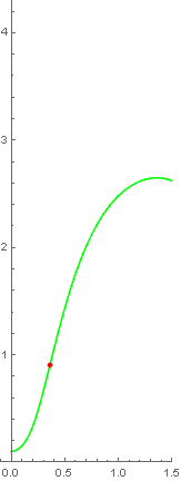
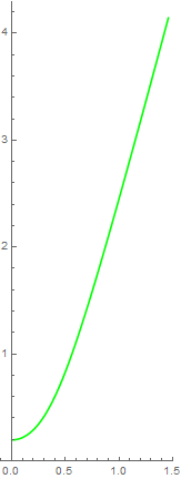
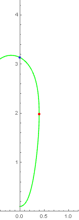
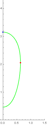
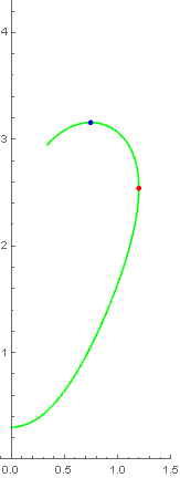
Figure 3.1.  Types of the profile curves.

We conclude this section by noting that if $\delta$ is the type 1.2, $x_{\delta}(s_{1})=0$ and $\theta_{\delta}(s_{1})=\pi$ by the definitions of $s_{1}$ and $s_{4}$. By the symmetry of system (2.6), these two equalities ensure that $\gamma_{\delta}(s)$, $0\leq s\leq 2s_{1}$ is a smooth simple closed profile curve, which will generate a $\lambda$-hypersurface diffeomorphic to $\mathbb{S}^{1}\times\mathbb{S}^{n-1}$. Also, if $\delta$ is the type 3, then $\gamma_{\delta}(s)$, $-\infty<s<\infty$ is simple and exits upper-half plane through infinity. Thus it will generate an embedded complete $\lambda$-hypersurface diffeomorphic to $\mathbb{R}\times\mathbb{S}^{n-1}$.

4. Behavior of the curve $\gamma_{\delta}$ when perturbing $\delta$

In this section, the behavior of the curve $\gamma_{\delta}$ when disturbing $\delta$ for each type or $\delta$ is near $0$ are studied. In particular, for the situations of near $0$ and the type 3, the geometric intuition is useful. We introduce the following variables (see [2, 8]):

$$\left\{\begin{aligned} \xi(t)&=\frac{1}{\delta}x(\delta\,t),\\ \rho(t)&=\frac{1}{\delta}(r(\delta\,t)-\delta),\\ \alpha(t)&=\theta(\delta\,t),\end{aligned}\right.$$

where $\delta>0$. From (2.6), they satisfy

(4.1) $$\left\{\begin{aligned} \xi^{\prime}&=\cos\alpha,\\ \rho^{\prime}&=\sin\alpha,\\ \alpha^{\prime}&=\frac{n-1}{1+\rho}\xi^{\prime}+\lambda\,\delta+\delta^{2}(\xi\,\rho^{\prime}-(1+\rho)\xi^{\prime}).\end{aligned}\right.$$

Consider the system (4.1) with initial conditions:

(4.2) $$\xi(0)=0,\ \ \rho(0)=0,\ \ \alpha(0)=0.$$

For $\delta=0$, this system can be solved explicitly, and one gets that $\alpha(t)=\arcsin\rho^{\prime}(t)$ , where $\rho(t)$ is the inverse function of

$$t=\int_{0}^{\rho}\frac{(1+\rho)^{n-1}}{\sqrt{(1+\rho)^{2(n-1)}-1}}{\rm d}\rho.$$

Since the solution of (4.1) depends smoothly on the parameter $\delta$, we may conclude the following.

Lemma 4.1.

For any $m\in\mathbb{N}^{*}$, there is a  $T_{m}>0$ and a  $\delta_{m}>0$ such that for all $0<\delta<\delta_{m}$, one has $T_{m}\,\delta<s_{2}(\delta)$, and at $s=T_{m}\,\delta$, $\arctan m<\theta_{\delta}<\pi/2$, $x_{\delta}=O(\delta)$ and $r_{\delta}=\delta+O(\delta)$. Where $\mathbb{N}^{*}$ denotes the set of positive natural numbers.

Remark 4.1.

For any fixed $m\in\mathbb{N}^{*}$, one can choose sufficiently small $\delta_{m}>0$ such that $x_{\delta}(T_{m}\,\delta)=O(\delta)<\frac{1}{m}$ and $r_{\delta}(T_{m}\,\delta)=\delta+O(\delta)<1$ for $0<\delta<\delta_{m}$. Consider the tangent line $l_{m,\delta}:r-r_{\delta}(T_{m}\,\delta)=\tan\theta_{\delta}(T_{m}\,\delta)(x-x_{\delta}(T_{m}\,\delta))$ of $\gamma_{\delta}$ at $s=T_{m}\,\delta$. Letting $r=1$ in the equation of $l_{m,\delta}$, we get

$$x=\frac{1}{\tan\theta_{\delta}(T_{m}\,\delta)}(1-O(\delta)-\delta)+O(\delta)<\frac{2}{m}$$

for $0<\delta<\delta_{m}$. Therefore, if $0<\delta<\delta_{m}$ and the profile curve $\gamma_{\delta}(s)=(x_{\delta},r_{\delta}),\ s\in(0,b]$ satisfies $\dot{r}_{\delta}>0$, $r_{\delta}\leq 1$ and $\dot{\theta}_{\delta}>0$ on $(0,b]$, one will have $x_{\delta}\leq\frac{2}{m}$ on $(0,b]$.

Henceforth we choose $\delta_{m}$ as in the above remark.

Lemma 4.2.

For $\lambda<0$, there exists $\bar{\delta}>0$ such that, for $0<\delta<\bar{\delta}$, $s_{1}(\delta)\leq s_{4}(\delta)$.

Proof.

Suppose that the statement is not true. For all $m\in\mathbb{N}^{*}$, there exist $0<\bar{\delta}_{m}<\min\left\{\frac{1}{m},\delta_{m}\right\}$ such that $s_{1}(\bar{\delta}_{m})>s_{4}(\bar{\delta}_{m})$. Putting $f_{m}(r)=f_{\bar{\delta}_{m}}(r)$ and $t_{m}=r_{\bar{\delta}_{m}}(s_{4}(\bar{\delta}_{m}))$. The proposition 3.1 implies that $\bar{\delta}_{m}$ is of the type 1 and

$$s_{2}(\bar{\delta}_{m})\geq s_{1}(\bar{\delta}_{m}),\ x_{\bar{\delta}_{m}}(s)>0\ {\rm in}\ (0,s_{4}(\bar{\delta}_{m})),$$

$$x_{\bar{\delta}_{m}}(s)<0\ {\rm in}\ (s_{4}(\bar{\delta}_{m}),s_{1}(\bar{\delta}_{m})),$$

$$\pi/2<\theta_{\bar{\delta}_{m}}(s)<\pi\ {\rm in}\ (s_{4}(\bar{\delta}_{m}),s_{1}(\bar{\delta}_{m})),\ {\rm and}\ \ r_{\bar{\delta}_{m}}(s_{1}({\bar{\delta}_{m}}))>R_{-\lambda}>\sqrt{n-1}.$$

Hence, we conclude

$$f^{\prime\prime}_{m}(r)<0\ {\rm in}\ (\bar{\delta}_{m},b_{\bar{\delta}_{m}}),$$

$$f_{m}(r)>0\ {\rm in}\ (\bar{\delta}_{m},t_{m}),\ \ f_{m}(r)<0\ {\rm in}\ (t_{m},b_{\bar{\delta}_{m}}),$$

$$f^{\prime}_{m}(r)<0\ {\rm in}\ (t_{m},b_{\bar{\delta}_{m}})\ {\rm and}\ \ b_{\bar{\delta}_{m}}>\sqrt{n-1}.$$

Next, we prove $t_{m}\rightarrow 0$ as $m\rightarrow\infty$. In fact, if this is not true, then there exists $\bar{\epsilon}>0$ such that for all $N>0$, there exists $m>N$ with $t_{m}>\bar{\epsilon}$. Therefore, one can choose a subsequence $\left\{m_{k}\right\}$ of the natural number sequence such that $f_{m_{k}}(r)>0$ on $(\bar{\delta}_{m_{k}},\bar{\epsilon}]$. Because of $f^{\prime\prime}_{m_{k}}(r)<0$ on $(\bar{\delta}_{m_{k}},\bar{\epsilon}]$, from the remark 4.1, we know that

$$f_{m_{k}}(r)<\frac{2}{m_{k}}\rightarrow 0\ \,{\rm as}\ \,k\to\infty$$

on $(\bar{\delta}_{m_{k}},\min\left\{1,\bar{\epsilon}\right\}]$. This implies that $f_{m_{k}}(r)$ converge to zero uniformly on a compact interval. One can find a sequence $\left\{\xi_{k}\right\}$ in a compact interval such that

$$\lim_{k\to\infty}f_{m_{k}}(\xi_{k})=0,\ \ \lim_{k\to\infty}f^{\prime}_{m_{k}}(\xi_{k})=0.$$

On the other hand, we know that the function $f_{m_{k}}(r)$ satisfies

$$\frac{f^{\prime\prime}_{m_{k}}}{1+(f^{\prime}_{m_{k}})^{2}}=(r-\frac{n-1}{r})f^{\prime}_{m_{k}}-f_{m_{k}}-\lambda\sqrt{1+(f^{\prime}_{m_{k}})^{2}}.$$

Letting $r=\xi_{k}$, we have

$$f^{\prime\prime}_{m_{k}}(\xi_{k})\to-\lambda>0\ \,{\rm as}\ \,k\to\infty,$$

which contradicts that $f^{\prime\prime}_{m_{k}}(r)<0$ on $(\bar{\delta}_{m_{k}},\bar{\epsilon}]$.
Choosing a positive $\epsilon<\sqrt{n-1}$ and large enough $m>0$, we have

$$f_{m}<0,\ \ f^{\prime}_{m}<0,\ \ f^{\prime\prime}_{m}<0$$

for $r\in(\epsilon,\sqrt{n-1})$. Since $f_{m}(r)$ satisfies

$$\frac{f^{\prime\prime}_{m}}{1+(f^{\prime}_{m})^{2}}=(r-\frac{n-1}{r})f^{\prime}_{m}-f_{m}-\lambda\sqrt{1+(f^{\prime}_{m})^{2}},$$

we know that it is impossible. This finishes the proof of the lemma. ∎

Proposition 4.1.

For $\lambda<0$, there exists $\hat{\delta}>0$ such that for $0<\delta<\hat{\delta}$, $\delta$ is the type 2, namely, $s_{2}(\delta)<s_{1}(\delta)$.

Proof.

Suppose that the assertion is not true. We have, for all $m\in\mathbb{N}^{*}$, there exist $0<\bar{\delta}_{m}<\min\left\{\frac{1}{m},\delta_{m}\right\}$ such that $s_{2}(\bar{\delta}_{m})\geq s_{1}(\bar{\delta}_{m})$. According to the lemma 4.2, we may assume $s_{4}(\bar{\delta}_{m})\geq s_{1}(\bar{\delta}_{m})$ without loss of generality. From the proposition 3.1, one obtain $\dot{\theta}_{\bar{\delta}_{m}}(s)>0$ in $(0,s_{1}(\bar{\delta}_{m}))$, $x_{\bar{\delta}_{m}}(s)>0$ in $(0,s_{1}(\bar{\delta}_{m}))$ and $r_{\bar{\delta}_{m}}(s_{1}(\bar{\delta}_{m}))>R_{-\lambda}>0$. Therefore, we have $f^{\prime\prime}_{\bar{\delta}_{m}}(r)<0$ in $(\bar{\delta}_{m},b_{\bar{\delta}_{m}})$, $f_{\bar{\delta}_{m}}(r)>0$ in $(\bar{\delta}_{m},b_{\bar{\delta}_{m}})$ and $b_{\bar{\delta}_{m}}>R_{-\lambda}>0$. By the same assertion as in the proof of the lemma 4.2, we will get a contradiction. ∎

Next we will describe the behavior of the curve $\gamma_{\delta}$ when perturbing $\delta$ of the type 3.

Lemma 4.3.

Assume $\lambda<0$ and that $\delta_{0}\in(0,R_{\lambda})$ is the type 3. We get $x_{\delta_{0}}(s_{1})=\infty$ and $r_{\delta_{0}}(s_{1})=\infty$.

Proof.

Since $\delta_{0}\in(0,R_{\lambda})$ is the type 3, $r_{\delta_{0}}(s_{1})=\infty$ has proved in the proposition 3.1. From $s_{1}=s_{3}$, we know that the curve $\gamma_{\delta_{0}}(s)$, $0<s<s_{1}$ can be written as a graph over $x$-axis. We denote this graph by $(x,u(x))$ where $0<x<x_{\delta_{0}}(s_{1})$. The function $u(x),\ 0<x<x_{\delta_{0}}(s_{1})$ is a right maximally extended solution of (2.7) by the definition of $s_{3}$. Furthermore, $u^{\prime}>0,\ u^{\prime\prime}>0$ in $(0,x_{\delta_{0}}(s_{1}))$ since $s_{1}=s_{2}=s_{3}$. Put $x_{\delta_{0}}(s_{1})=b$. We also point out that $b>-\lambda$. Otherwise $\dot{\theta}_{\delta_{0}}<0$ as $s$ approaches $s_{1}$ due to

$$\dot{\theta}_{\delta_{0}}=(\frac{n-1}{r_{\delta_{0}}}-r_{\delta_{0}})\cos\theta_{\delta_{0}}+x_{\delta_{0}}\,\sin\theta_{\delta_{0}}+\lambda,$$

$r_{\delta_{0}}(s_{1})=\infty$ and $\lambda<0$.
If $b<\infty$, we have $\lim_{x\to b^{-}}u^{\prime}(x)=\infty$. For $\tilde{\lambda}$ with $-\lambda<-\tilde{\lambda}<b$, there exists $x_{1}\in(-\tilde{\lambda},b)$ such that $(x+\tilde{\lambda})u^{\prime}-u>0$ for $x\in(x_{1},b)$ since $\lim_{x\rightarrow b^{-}}((x+\tilde{\lambda})u^{\prime}(x)-u(x))=\infty$ when $\lim_{x\to b^{-}}u^{\prime}(x)=\infty$. Furthermore, there exists $x_{2}\in(-\tilde{\lambda},b)$ such that $\sqrt{1+u^{\prime}(x)^{2}}<\frac{\tilde{\lambda}}{\lambda}u^{\prime}(x)$ for $x\in(x_{2},b)$ due to $\lim_{x\to b^{-}}u^{\prime}(x)=\infty$.
Therefore, we have

$$\dfrac{u^{\prime\prime}}{1+(u^{\prime})^{2}}=xu^{\prime}-u+\dfrac{n-1}{u}+\lambda\sqrt{1+(u^{\prime})^{2}}>xu^{\prime}-u+\dfrac{n-1}{u}+\tilde{\lambda}u^{\prime}>\dfrac{n-1}{u}$$

for $x>\max\left\{x_{1},x_{2}\right\}$. From a direct calculation, we obtain

$$\dfrac{u^{\prime\prime\prime}}{1+(u^{\prime})^{2}} =\dfrac{2u^{\prime}(u^{\prime\prime})^{2}}{(1+(u^{\prime})^{2})^{2}}-\dfrac{n-1}{u^{2}}u^{\prime}+xu^{\prime\prime}+\lambda\dfrac{u^{\prime}u^{\prime\prime}}{\sqrt{1+(u^{\prime})^{2}}}$$

$$>2u^{\prime}\dfrac{(n-1)^{2}}{u^{2}}-\dfrac{n-1}{u^{2}}u^{\prime}+xu^{\prime\prime}+\tilde{\lambda}\dfrac{u^{\prime}u^{\prime\prime}}{\sqrt{1+(u^{\prime})^{2}}}$$

$$>(x+\tilde{\lambda})u^{\prime\prime}$$

$$>(\max\left\{x_{1},x_{2}\right\}+\tilde{\lambda})u^{\prime\prime}$$

for $x>\max\left\{x_{1},x_{2}\right\}$. Thus, letting $\phi=u^{\prime}$, one has

$$\phi^{\prime\prime}=u^{\prime\prime\prime}>(\max\left\{x_{1},x_{2}\right\}+\tilde{\lambda})\phi^{\prime}\phi^{2}$$

for $x>\max\left\{x_{1},x_{2}\right\}$.
For small $\epsilon>0$, we consider the function

$$\phi_{\epsilon}(x)=\dfrac{M}{\sqrt{b-\epsilon-x}}.$$

By choose a sufficient large $M>0$ such that $\phi(\max\left\{x_{1},x_{2}\right\})\leq\dfrac{M}{\sqrt{b-\max\left\{x_{1},x_{2}\right\}}}$ and $\dfrac{3}{2M^{2}}\leq\max\left\{x_{1},x_{2}\right\}+\tilde{\lambda}$, we have

$$\phi_{\epsilon}^{\prime\prime}\leq(\max\left\{x_{1},x_{2}\right\}+\tilde{\lambda})\phi_{\epsilon}^{\prime}\phi_{\epsilon}^{2},$$

$$\phi_{\epsilon}(\max\left\{x_{1},x_{2}\right\})>\phi(\max\left\{x_{1},x_{2}\right\}).$$

If $\phi_{\epsilon}-\phi$ is negative at some point in $(\max\left\{x_{1},x_{2}\right\},b-\epsilon)$, from $\phi_{\epsilon}(\max\left\{x_{1},x_{2}\right\})>\phi(\max\left\{x_{1},x_{2}\right\})$ and $\phi_{\epsilon}(b-\epsilon)=\infty$, we know that $\phi_{\epsilon}-\phi$ achieves a negative minimum at some point $x_{0}\in(\max\left\{x_{1},x_{2}\right\},b-\epsilon)$. By computing $(\phi_{\epsilon}-\phi)^{\prime\prime}$ at $x_{0}$, we conclude

$$0\leq(\phi_{\epsilon}-\phi)^{\prime\prime}\leq(\max\left\{x_{1},x_{2}\right\}+\tilde{\lambda})\phi_{\epsilon}^{\prime}(x_{0})(\phi_{\epsilon}(x_{0})^{2}-\phi(x_{0})^{2})<0.$$

This is impossible. Therefore $\phi\leq\phi_{\epsilon}$. By integrating and taking $\epsilon\to 0$, we see that $u(b)$ is finite, which contradicts $r_{\delta_{0}}(s_{1})=\infty$. Hence, we get $x_{\delta_{0}}(s_{1})=\infty$ ∎

Proposition 4.2.

For $\lambda<0$, if $\delta_{0}\in(0,R_{\lambda})$ is the type 3, there exists $\epsilon>0$ such that $s_{4}(\delta)\geq s_{1}(\delta)$ provided $\delta$ is the type 1 and $\delta\in(\delta_{0}-\epsilon,\delta_{0}+\epsilon)$.

Proof.

By the proposition 3.1 and the lemma 4.3, one can choose $T$: $0<T<s_{2}=s_{3}$ such that $\dot{\theta}_{\delta_{0}}(s)>0$ in $[0,T]$ and

$$\theta_{\delta_{0}}(T)<\pi/2,$$

$$x_{\delta_{0}}(T)>\sqrt{2}(\pi+|\lambda|)+1,$$

$$r_{\delta_{0}}(T)>\dfrac{\sqrt{2}(\pi+|\lambda|)+\sqrt{2(\pi+|\lambda|)^{2}+4(n-1)}}{2}+1.$$

Since the solution of ordinary equations continuously depend on the initial datas, there exists $\epsilon>0$ such that the above three inequalities hold for $\delta\in(\delta_{0}-\epsilon,\delta_{0}+\epsilon)$. Therefore $0<\theta_{\delta}(s)<\pi/2$ in $(0,T]$ and

$$T<s_{3}(\delta),$$

$$x_{\delta}(s_{3}(\delta))>\sqrt{2}(\pi+|\lambda|)+1,$$

$$r_{\delta}(s_{3}(\delta))>\dfrac{\sqrt{2}(\pi+|\lambda|)+\sqrt{2(\pi+|\lambda|)^{2}+4(n-1)}}{2}+1.$$

for $\delta\in(\delta_{0}-\epsilon,\delta_{0}+\epsilon)$.
If $\delta\in(\delta_{0}-\epsilon,\delta_{0}+\epsilon)$ is the type 1, we can prove $s_{4}\geq s_{1}$. In fact, for simple, we denote $s_{1}(\delta)$ by $s_{1}$ and so on. Suppose $s_{4}<s_{1}$. We know $x_{\delta}(s_{4})=0$. Since $\delta$ is the type 1, $s_{1}>s_{3}$ and $\dot{\theta}_{\delta}(s)>0$ in $[0,s_{1})$. We further indicate that $s_{4}-s_{3}>1$. Otherwise $x_{\delta}(s_{3})=\left|x_{\delta}(s_{4})-x_{\delta}(s_{3})\right|=\left|\int_{s_{3}}^{s_{4}}\cos\theta_{\delta}(\xi){\rm d}\xi\right|\leq 1$. Hence, $(0,s_{1})\supset[s_{3},s_{3}+1]$, in which

$$x_{\delta}(s)>\sqrt{2}(\pi+|\lambda|),$$

$$r_{\delta}(s)>\dfrac{\sqrt{2}(\pi+|\lambda|)+\sqrt{2(\pi+|\lambda|)^{2}+4(n-1)}}{2}$$

according to the lower bounds for $x_{\delta}(s_{3})$ and $r_{\delta}(s_{3})$. Thus, the above last inequality implies

$$\dfrac{n-1}{r_{\delta}}-r_{\delta}<-\sqrt{2}(\pi+|\lambda|).$$

If $\theta_{\delta}\neq\dfrac{3\pi}{4}$ in $(s_{3},s_{3}+\dfrac{1}{2})$, we can infer, for $s\in(s_{3},s_{3}+\dfrac{1}{2})$,

$$\dfrac{\pi}{2}\leq\theta_{\delta}(s)\leq\dfrac{3\pi}{4},$$

$$\sin\theta_{\delta}(s)\geq\dfrac{\sqrt{2}}{2},$$

$$\dot{\theta}_{\delta}(s)=(\frac{n-1}{r_{\delta}}-r_{\delta})\,\cos\theta_{\delta}+x_{\delta}\,\sin\theta_{\delta}+\lambda$$

$$>\sqrt{2}\,(\pi+|\lambda|)\,\dfrac{\sqrt{2}}{2}+\lambda=\pi.$$

We obtain

$$\theta_{\delta}(s_{3}+\dfrac{1}{2})-\theta_{\delta}(s_{3})=\int_{s_{3}}^{s_{3}+1/2}\dot{\theta}_{\delta}(s){\rm d}s>\dfrac{\pi}{2},$$

which contradicts $s_{3}+\dfrac{1}{2}<s_{1}$.
Thus, there exists an $s$ in $(s_{3},s_{3}+\dfrac{1}{2})$ such that $\theta_{\delta}=\dfrac{3\pi}{4}$. We have for $s\in[s_{3}+\dfrac{1}{2},s_{3}+1]$,

$$\dfrac{3\pi}{4}<\theta_{\delta}(s)<\pi,$$

$$\cos\theta_{\delta}(s)<-\dfrac{\sqrt{2}}{2},$$

$$\dot{\theta}_{\delta}(s)>\sqrt{2}\,(\pi+|\lambda|)\,\dfrac{\sqrt{2}}{2}+\lambda=\pi.$$

We derive

$$\theta_{\delta}(s_{3}+1)-\theta_{\delta}(s_{3}+\dfrac{1}{2})=\int_{s_{3}+1/2}^{s_{3}+1}\dot{\theta}_{\delta}(s){\rm d}s>\dfrac{\pi}{2},$$

which also contradicts $s_{3}+1<s_{1}$. Hence, we get $s_{4}\geq s_{1}$. ∎

Lemma 4.4.

If $\delta_{0}$ in $(0,R_{\lambda})$ is the type 1, the type 2, the type1.1 or the type 1.3, then there exists $\epsilon>0$ such that $\delta$ in $(\delta_{0}-\epsilon,\delta_{0}+\epsilon)$ is the same type.

Proof.

Assume that $\delta_{0}$ is the type 1. We can choose $T$ such that $s_{3}(\delta_{0})<T<s_{1}(\delta_{0})$, $\pi/2<\theta_{\delta_{0}}(T)<\pi$ and $\dot{\theta}_{\delta_{0}}(s)>0$ in $[0,T]$ from the proposition 3.1. Since solutions of ordinary equations continuously depend on the initial datas, there exists $\epsilon>0$ such that $\pi/2<\theta_{\delta}(T)<\pi$ and $\dot{\theta}_{\delta}(s)>0$ in $[0,T]$ for $\delta\in(\delta_{0}-\epsilon,\delta_{0}+\epsilon)$. Therefore $0<\theta_{\delta}(s)<\pi$ in $(0,T]$ and $T<s_{1}(\delta)$. Moreover for $\delta\in(\delta_{0}-\epsilon,\delta_{0}+\epsilon)$, there exists an $s$ in $(0,T)$ at which $\theta_{\delta}=\pi/2$ from the intermediate value theorem. Thus for $\delta\in(\delta_{0}-\epsilon,\delta_{0}+\epsilon)$ one has $s_{3}(\delta)<T<s_{1}(\delta)$, namely, $\delta$ is the type 1. We actually proved that $s_{3}(\delta)<T<s_{1}(\delta)$ is equivalent to $\pi/2<\theta_{\delta}(T)<\pi$ and $\dot{\theta}_{\delta}(s)>0$ in $[0,T]$. For the other cases, we can prove them in the same way as in the type 1. ∎

5. Proof of the theorems

From the proposition 4.1, we know that $\delta$ nearing $0$ is the type 2 for $\lambda<0$. We need to show that there exists a ${\delta^{*}}$ in $(0,R_{\lambda})$ such that it is not the type 2.

Lemma 5.1.

Given $0<\delta^{*}<\sqrt{n-1}$, there exists $\bar{\lambda}(\delta^{*})<0$ such that $\delta^{*}$ is the type 1 for $\bar{\lambda}(\delta^{*})<\lambda\leq 0$. Moreover, one can choose $0<\delta_{1}^{*}<\sqrt{n-1}$ such that $\delta_{1}^{*}$ is the type 1.1 for $\bar{\lambda}(\delta_{1}^{*})<\lambda\leq 0$. One can also choose $\delta_{1}^{*}<\delta_{2}^{*}<\sqrt{n-1}$ such that $\delta_{2}^{*}$ is the type 1.3 for $\bar{\lambda}(\delta_{2}^{*})<\lambda\leq 0$.

Proof.

If $\lambda=0$, Drugan and Kleene [12] showed that $\delta^{*}$ is the type 1 for $0<\delta^{*}<\sqrt{n-1}$. In particular, $\delta^{*}$ is the type 1.1 for $\delta^{*}$ close to $0$, $\delta^{*}$ is the type 1.3 for $\delta^{*}$ close to $\sqrt{n-1}$ from below. Since the solution of (2.6) depends smoothly on the parameter $\lambda$, the proof of this lemma is similar to the proof of lemma 4.4. ∎

Note that $\bar{\lambda}(\delta^{*})$ only depends on $n$ and $\delta^{*}$. Now we can prove the theorem 1.1 and the theorem 1.2.

Proof of Theorem 1.1. Given $\mu$ in $(\bar{\lambda}(\sqrt{n-1}/2),0)$ where $\bar{\lambda}(\sqrt{n-1}/2)$ is as in the lemma 5.1, we consider the the set

$$\left\{\tilde{\delta}\in(0,R_{\mu}):\forall\delta\in(0,\tilde{\delta}),\ \delta\ {\rm is\ the\ type\ 2}\right\}$$

which is non-empty by the proposition 4.1. Following the argument in [8] (cf. [2]). We define $\delta_{c}$ as the supremum of this set:

$$\delta_{c}=\sup\left\{\tilde{\delta}\in(0,R_{\mu}):\forall\delta\in(0,\tilde{\delta}),\ \delta\ {\rm is\ the\ type\ 2}\right\}.$$

Then $\delta_{c}\leq R_{\mu}$ and $\delta_{c}$ is the largest real number in $(0,R_{\mu}]$ such that $\delta$ is the type 2 for all $\delta\in(0,\delta_{c})$. But the lemma 5.1 shows that $\delta_{c}<R_{\mu}$ for $\bar{\lambda}(\sqrt{n-1}/2)<\mu<0$ and then, by the definition of $\delta_{c}$, we can further utilize the lemma 4.4 to obtain that $\delta_{c}$ is neither the type 1 nor the type 2. Hence, $\delta_{c}$ is the type 3 (see the red curve in figure 5.15.1). Then the profile curve $\gamma_{\delta_{c}}(s)$, $-\infty<s<\infty$ generates an embedded complete $\mu$-hypersurface diffeomorphic to $\mathbb{R}\times\mathbb{S}^{n-1}$. Letting $\lambda=-\mu$, switching the unit normal vector to its opposite, we obtain a $\lambda$-hypersurface which is non-convex by (2.3). This completes the proof of the theorem 1.1. A $\lambda$-cylinder in $\mathbb{R}^{3}$ with $\lambda=0.4$ is shown in figure 5.2.

We should remark why we switch the unit normal vector because of the following reason. The hypersurface constructed in theorem 1.1 is rotationally invariant, it can be regarded as a deformation of the standard cylinder. So we may think that the normal vector pointing to the axis is inward like the case of standard cylinder. From this point of view, the unit normal vector we choose in (2.2) is outward.

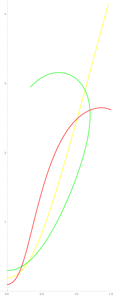
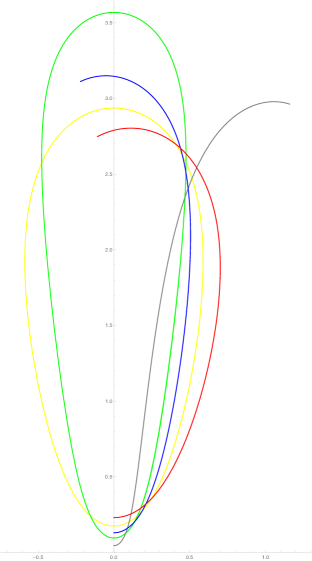
Figure 5.1.  The profile curves of the $\lambda$-hypersurfaces. In subfigure (a), $n=2$, $\lambda=0.4$. In subfigure (b), $n=2$, $\lambda=-0.24$.

Proof of Theorem 1.2. Given $\lambda$ in $(\max\left\{\bar{\lambda}(\delta_{1}^{*}),\bar{\lambda}(\delta_{2}^{*})\right\},0)$ where $\bar{\lambda}(\delta_{1}^{*})$ and $\bar{\lambda}(\delta_{2}^{*})$ are as in lemma 5.1, we consider the the set

$$\left\{\delta\in(0,\delta_{2}^{*}):\delta\ {\rm is\ of\ type\ 1.1}\right\}$$

which is non-empty by the lemma 5.1. Define

$$\delta_{t_{1}}=\inf\left\{\delta\in(0,\delta_{2}^{*}):\delta\ {\rm is\ of\ type\ 1.1}\right\}$$

and

$$\delta_{t_{2}}=\sup\left\{\delta\in(0,\delta_{2}^{*}):\delta\ {\rm is\ of\ type\ 1.1}\right\}.$$

The proposition 4.1 shows that ${\delta_{t_{1}}}>0$. Therefore we can further utilize the lemma 4.4 and the proposition 4.2 to obtain that $\delta_{t_{1}}$ is neither of type 1.1, type 1.3, type 2 nor of type 3. In other words, $\delta_{t_{1}}$ is of type 1.2 (see the green curve in figure 5.15.1). Similar argument will prove that $\delta_{t_{2}}$ is of type 1.2 (see the yellow curve in figure 5.15.1). This completes the proof of theorem 1.2. Two $\lambda$-tori in $\mathbb{R}^{3}$ with $\lambda=-0.24$ are shown in figure 5.3.

Remark 5.1.

Numerical evidence shows that $\delta$ in $(0,R_{\mu_{1}})$ may all be of type 1 for $\mu_{1}>0$, so the examples in theorem 1.1 may not exist for $\lambda<0$. Numerical evidence also shows that $\delta$ in $(0,R_{\mu_{2}})$ may all be of type 2 for $\mu_{2}<0$ close to $-\infty$, so the examples in theorem 1.1 may not exist for $\lambda>0$ close to $\infty$, the examples in theorem 1.2 may not exist for $\lambda<0$ close to $-\infty$.

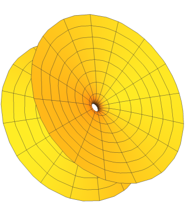
Figure 5.2.  A $\lambda$-cylinder in $\mathbb{R}^{3}$ where $\lambda=0.4$.

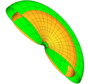
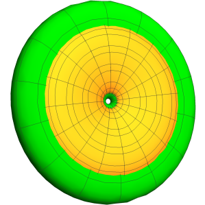
Figure 5.3.  Two $\lambda$-tori in $\mathbb{R}^{3}$ where $\lambda=-0.24$.

References

- [1] H. Alencar, G. Silva Neto and D. Zhou, Hopf-type theorem for self-shrinkers, J. Reine Angew. Math. 782 (2022), 247-279.
- [2] S. B. Angenent, Shrinking doughnuts Birkhäuser, Boston-Basel-Berlin, 7, 21-38, 1992.
- [3] S. Brendle, Embedded self-similar shrinkers of genus 0, Ann. of Math. 183 (2016), 715-728.
- [4] J. -E. Chang, 1-dimensional solutions of the -self shrinkers, Geom. Dedicata 189 (2017), 97-112.
- [5] T. H. Colding and W. P. Minicozzi II, Generic mean curvature flow I; generic singularities, Ann. of Math. 175 (2012), 755-833.
- [6] A. C. -P. Chu and A. Sun, Genus one singularities in the mean curvature flow, arXiv: 2308.05923v1. 2023.
- [7] Q. -M. Cheng and G. Wei, Complete -hypersurfaces of weighted volume-preserving mean curvature flow, Cal. Var. Partial Differential Equations 57 (2018), 32.
- [8] Q. -M. Cheng and G. Wei, Examples of compact -hypersurfaces in Euclidean spaces, Sci. China Math. 64 (2021), 155-166.
- [9] Q. -M. Cheng, J. Lai and G. Wei, Examples of compact embedded convex -hypersurfaces, J. Funct. Anal. 286 (2024), no. 2, Paper No. 110211.
- [10] M. do Carmo and M. Dajczer, Hypersurfaces in space of constant curvature, Trans. Amer. Math. Soc. 277 (1983), 685-709.
- [11] G. Drugan, An immersed self-shrinker. Trans. Amer. Math. Soc. 367 (2015), 3139-3159.
- [12] G. Drugan and S. J. Kleene, Immersed self-shrinkers, Trans. Amer. Math. Soc. 369 (2017), 7213-7250.
- [13] Q. Guang, A note on mean convex -surfaces in , Proc. Amer. Math. Soc. 149 (2021), 1259-1266.
- [14] S. Heilman, Symmetric convex sets with minimal Gaussian surface area, Amer. J. Math. 143 (2021), 53-94.
- [15] T. Ilmanen, Problems in mean curvature flow, Available at http://people.math.ethz.ch/ ilmanen/classes/eil03/problems03.pdf.
- [16] S. Kleene and N. M. Møller, Self-shrinkers with a rotational symmetry, Trans. Amer. Math. Soc. 366 (2014), no. 8, 3943-3963.
- [17] T. -K. Lee, Convexity of -hypersurfaces, Proc. Amer. Math. Soc. 150 (2022), 1735-1744.
- [18] Z. Li and G. Wei, An immersed -hypersurface, J. Geom. Anal. 33 (2023), Paper No. 288, 29 pp.
- [19] P. McGrath, Closed mean curvature self-shrinking surfaces of generalized rotational type, arXiv: 1507.00681. 2015.
- [20] M. McGonagle and J. Ross, The hyperplane is the only stable, smooth solution to the isoperimetric problem in Gaussian space, Geom. Dedicata 178 (2015), 277-296.
- [21] J. Ross, On the existence of a closed, embedded, rotational -hypersurface, J. Geom. 110 (2019), 1-12.
- [22] O. Riedler, Closed Embedded Self-shrinkers of Mean Curvature Flow, J. Geom. Anal. 33 (2023), 172.
- [23] A. Sun, Compactness and rigidity of -surfaces, Math. Res. Not. IMRN (2021), no. 15, 11818-11844.