All-electron BSE@GW method with Numeric Atom-Centered Orbitals for Extended Systems

Abstract

Green’s function theory has emerged as a powerful many-body approach not only in condensed matter physics but also in quantum chemistry in recent years. We have developed a new all-electron implementation of the BSE@GW formalism using numeric atom-centered orbital basis sets (Liu et al., J. Chem. Phys. 152, 044105 (2020)). We present our recent developments in implementing this formalism for extended systems with periodic boundary conditions. We discuss its numerical implementation and various convergence tests pertaining to numerical atom-centered orbitals, auxiliary basis sets for the resolution-of-identity formalism, and Brillouin zone sampling. Several proof-of-principle examples are presented to compare with other formalisms, illustrating the new all-electron BSE@GW method for extended systems.

Thomas Lord Department of Mechanical Engineering and Materials Science, Duke University, Durham, North Carolina 27708, USA Thomas Lord Department of Mechanical Engineering and Materials Science, Duke University, Durham, North Carolina 27708, USA Department of Chemistry, Duke University, Durham, North Carolina 27708, USA Department of Physics and Astronomy, University of North Carolina at Chapel Hill, Chapel Hill, North Carolina 27599, USA

1 1.Introduction

In the last decade, the many-body perturbation theory based on Green’s function formalism has found its way into chemistry community from condensed matter physics community. By going beyond well-accepted approximations for condensed matter systems (e.g. plasmon-pole approximation, etc), a number of groups have shown that the so-called $GW$ and Bethe-Salpeter equation (BSE) methods can be made quite promising for studying excited state properties of isolated molecules ^{1, 2, 3, 4}. Solving the particle-hole two-particle Green’s function, the BSE method ^{5, 6, 7, 8} has become increasingly popular for calculating neutral excitations of molecules in recent years ⁴, adding to a history of successes for condensed matter systems^{9, 10, 11}. It is now widely recognized as a promising alternative^{12, 13, 14} to density functional theory (DFT)-based approaches such as linear-response time-dependent density function theory (LR-TDDFT)^{15, 16} and traditional wavefunction-based methods like the equation-of-motion coupled cluster (EOM-CC) ^{17, 18}.

The BSE method is based on the many-body perturbation theory in the Green’s function ($G$) framework, and the screened Coulomb interaction, $W$, is used to model the interaction between the excited electron and hole. Combined with the $GW$ approximation to the self-energy, the BSE method has been shown to successfully yield the optical spectra of solids and nano-structured systems, and more recent work also shows similar applicability to low-energy electronic excitation of molecular systems ^{19, 20, 21, 22, 23}. The BSE@$GW$ approach yields the accuracy of 0.1-0.2 eV, being comparable to the EOM-CCSD ^{13, 14}. Due to its favorable scaling of $N^{4}$ in terms of the number of electrons, the approach is highly promising for studying excited-state properties of increasingly complex systems. Our previous work has also shown that all-electron BSE@$GW$ method using atom-centered orbital basis sets gives great accuracy for modeling core-electron excitations, comparable to the state-of-the-art EOM-CCSD method²⁴. Such computational capability to quantitatively predict X-ray absorption spectra of molecules is of great interest as many light-source facilities have undergone great advancement in recent years.

Building on our recent effort on developing all-electron many-body perturbation theory methods using the numeric atom-centered orbitals as the basis set (e.g. $GW$ methods for extended periodic systems ²⁵ and BSE for isolated systems ^{26, 24}), we here extend the BSE@$GW$ approach to periodic systems with the Brillouin zone integration. For studying the extended systems, taking into account the dependence on the reciprocal wave vector requires careful consideration as we develop the formalism based on the atom-centered basis set. Most $GW$/BSE method developments originating in condensed matter physics are based on plane-waves or real-space-grids with non-local pseudo-potentials, and the numerical formulations of these Green’s function methods are largely incompatible with the mathematical/numerical frameworks used in many quantum-chemistry developments/codes. The new theoretical method and algorithm will benefit the quantum chemistry field which is largely based on all-electron implementation with atom-centered basis functions like Gaussian-type orbitals. Our development here will enable the quantum chemistry community to take advantage of recent exciting advances in the Green’s function theory methods and promote further synergies with traditional post-Hartree-Fock methods.

2 2. Green’s Function Theory

2.1 2.1 Bethe Salpeter Equation

For describing electron-hole pairs in a many-electron system, the two-body correlation function plays a central role in many-body perturbation theory based on Green’s function. One-body Green’s function $G_{1}$ and two-body Green’s function $G_{2}$ are defined as

$$iG_{1}(1,2)=\langle N,0|T[\hat{\psi}(1)\hat{\psi}^{\dagger}(2)]|N,0\rangle$$ (1)

$$i^{2}G_{2}(1,2;1^{\prime},2^{\prime})=\langle N,0|T[\hat{\psi}(1)[\hat{\psi}(2)\hat{\psi}^{\dagger}(2^{\prime})\hat{\psi}^{\dagger}(1^{\prime})]|N,0\rangle$$ (2)

where the creation operator $\hat{\psi}(1)$ and the annihilation operator $\hat{\psi}^{\dagger}(2)$ are the field operators written in the Heisenberg picture: $\hat{\psi}(1)=e^{i\hat{H}t_{1}}\hat{\psi}(\mathbf{x_{1})}e^{-i\hat{H}t_{1}}$ and $\hat{\psi}^{\dagger}(2)=e^{i\hat{H}t_{2}}\hat{\psi}^{\dagger}(\mathbf{x_{2}})e^{-i\hat{H}t_{2}}$. $1\equiv(x_{1},t_{1})$, $2\equiv(x_{2},t_{2})$ denoting a composite variable encompassing space, spin, and time. Here, $|N,0\rangle$ is the ground state state for N-electron system and $T$ is the time ordering operator. The correlation function, $\cal L$, is formally given as a functional derivative of one-body Green’s function $G(1,1^{\prime})$ with respect to an external non-local perturbation $U(2^{\prime},2)$,

$${\cal L}(1,2;1^{\prime},2^{\prime})=\frac{\delta G(1,1^{\prime})}{\delta U(2^{\prime},2)}$$ (3)

In terms of the Greens’ functions, it is expressed as

$${\cal L}(1,2;1^{\prime},2^{\prime})=-G_{2}(1,2;1^{\prime},2^{\prime})+G_{1}(1,1^{\prime})G_{1}(2,2^{\prime})$$ (4)

${\cal L}(1,2;1^{\prime},2^{\prime})$ describes the probability amplitude of an electron propagating from $1^{\prime}$ to $2$ and a hole propagating from $1$ to $2^{\prime}$. By incorporating Eqn. 1 and Eqn. 2 into Eqn. 4 and using the completeness property of N-electron system in an excited state $m$ $|N,m\rangle$ (i.e. $\sum_{m}|N,m\rangle\langle N,m|=I$), we can expand the correlation function as following:

$${\cal L}(\mathbf{x_{1}},\mathbf{x_{2}};\mathbf{x_{1}^{\prime}},\mathbf{x_{2}^{\prime}};\tau) =\theta(\tau)\sum_{m\neq 0}\langle N,0|\hat{\psi}^{\dagger}(\mathbf{x_{1}^{\prime}})\hat{\psi}(\mathbf{x_{1}})|N,m\rangle\langle N,m|\hat{\psi}^{\dagger}(\mathbf{x_{2}^{\prime}})\hat{\psi}(\mathbf{x_{2}})|N,0\rangle e^{-i(E_{N,n}-E_{N,0})\tau}$$ (5)

$$+\theta(-\tau)\sum_{m\neq 0}\langle N,0|\hat{\psi}^{\dagger}(\mathbf{x_{2}^{\prime}})\hat{\psi}(\mathbf{x_{2}})|N,m\rangle\langle N,m|\hat{\psi}^{\dagger}(\mathbf{x_{1}^{\prime}})\hat{\psi}(\mathbf{x_{1}})|N,0\rangle e^{i(E_{N,m}-E_{N,0})\tau}$$

where $E_{N,m}$ is the energy for $|N,m\rangle$. By employing Fourier transformation, we arrive at the Lehmann representation of the two-body correlation function $\cal L$ within the frequency domain

$${\cal L}\left(\mathbf{x_{1}},\mathbf{x_{2}};\mathbf{x_{1}^{\prime}},\mathbf{x_{2}^{\prime}};\omega\right)=i\sum_{n\neq 0}[\frac{{A_{n}(\mathbf{x_{1}},\mathbf{x_{1}^{\prime}})}A^{*}_{m}(\mathbf{x_{2}^{\prime},\mathbf{x_{2}})}}{\omega-\omega_{m}+i0^{+}}-\frac{{A_{n}(\mathbf{x_{2}},\mathbf{x_{2}^{\prime}})}A^{*}_{m}(\mathbf{x_{1}}^{\prime},\mathbf{x_{1}})}{\omega+\omega_{m}-i0^{+}}]$$ (6)

where $0^{+}$ is a positive infinitesimal, $A_{m}$ represents the amplitude associated with the coupled electron-hole pair for m-th excited state:$A_{m}(\mathbf{x},\mathbf{x^{\prime}})=-\langle N,0|\hat{\psi}^{\dagger}(\mathbf{x})\hat{\psi}(\mathbf{x}^{\prime})|N,m\rangle$ and $\omega_{m}$ corresponds to the excitation energy from the ground state to the m-th excited state $\omega_{m}=E_{N,m}-E_{N,0}$.

Bethe-Salpeter equation (BSE) relates the two-body correlation function to the non-interacting one as²⁷

$${\cal L}(1,2;1^{\prime},2^{\prime})={\cal L}_{0}(1,2;1^{\prime},2^{\prime})+\int d(3456){\cal L}_{0}(1,4;1^{\prime},3)K(3,5;4,6){\cal L}(6,2;5,2^{\prime})$$ (7)

where ${\cal L}_{0}(1,2;1^{\prime},2^{\prime})$ is non-interacting correlation function, given by

$${\cal L}_{0}(1,2;1^{\prime},2^{\prime})=G_{1}(1,2^{\prime})G_{1}(2,1^{\prime}).$$ (8)

The electron-hole interaction kernel, $K(35;46)$, is defined as

$$K(3,4;5,6)=\frac{\delta[v_{H}(3)\delta(3,4)+\Sigma(3,4)]}{\delta G(6,5)}$$ (9)

where $v_{H}(1)=-i\int d2v(1,2)G(2,2^{+})$ is the Hartree potential and $\Sigma(3,4)$ is the self-energy. $1^{+}$ is used to indicates $t_{1}^{+}=t_{1}+0^{+}$. By adopting the widely-used $GW$ approximation²⁸ to the self-energy $\Sigma(3,4)=iG(3,4)W(3,4)$, the kernel simplifies to²⁹,

$$K(3,4;5,6)=-i\delta(3,4)\delta(5^{-},6)v(3,6)+i\delta(3,6)\delta(4,5)W(3^{+},4;\omega)$$ (10)

where $\delta$ represents Dirac delta function. Although the frequency dependence of $W$ have been considered in solving BSE^{29, 30, 31}, most standard implementations adapt the so-called static screening effect approximation by neglecting the frequency dependence ²⁹ such that Eq. 10 reduces to

$$K(\textbf{r}_{3},\textbf{r}_{5},\textbf{r}_{4},\textbf{r}_{6})=-iv(\textbf{r}_{3}-\textbf{r}_{5})\delta(\textbf{r}_{3}-\textbf{r}_{4})\delta(\textbf{r}_{5}-\textbf{r}_{6})+iW(\textbf{r}_{3},\textbf{r}_{4})\delta(\textbf{r}_{3}-\textbf{r}_{6})\delta(\textbf{r}_{4}-\textbf{r}_{5})$$ (11)

In our subsequent discussion, we use the notation $W$ to represent the static screened interaction in the limit of $\omega=0$ for brevity. The BSE interaction kernel includes two physically distinct terms, the bare Coulomb interaction and the static screened exchange interaction. In the limit where the parameter W approaches the value of $v$ as the dielectric term $\epsilon$ approaches one, the second term precisely recovers the bare exchange term within the Hartree-Fock approximation.

2.2 2.2 Bethe Salpeter Equation as Eigenvalue Problem

For first-principles theory implementation of BSE, it is convenient to write the BSE amplitudes in Eq. 6 in terms of the particle-hole basis,

$$A_{m}(\mathbf{x},\mathbf{x^{\prime}})=\sum_{vc}X_{vc,m}\psi_{c}(\mathbf{x})\psi_{v}(\mathbf{x^{\prime}})+Y_{cv,m}\psi_{v}(\mathbf{x})\psi_{c}(\mathbf{x^{\prime}})$$ (12)

where $\psi_{c}$ and $\psi_{v}$ represent single-particle orbitals of the conduction band (i.e. unoccupied) and valence band (i.e. occupied), respectively. $\psi_{c}(\mathbf{x})\psi_{v}(\mathbf{x^{\prime}})$ and $\psi_{v}(\mathbf{x})\psi_{c}(\mathbf{x^{\prime}})$ represent the particle-hole basis functions, and they correspond to resonant and anti-resonant transitions of electron-hole pairs, respectively. Typically, by adapting $G_{0}W_{0}$ approximation for the self-energy calculation, the orbitals from mean-field theories such as Hartree-Fock (HF) and Kohn-Sham density functional theory (KS-DFT) are used for the single-particle orbitals in practice. Thus, the matrices $X$ and $Y$ represent the solutions to the BSE, which needs to be solved.

The non-interacting correlation function ${\cal L}_{0}$ (Eq. 8) can be written using the Lehmann representation, analogously to the derivation of Eq. 6 from Eq. 5,

$${\cal L}_{0}\left(\mathbf{x_{1}},\mathbf{x_{2}};\mathbf{x_{1}^{\prime}},\mathbf{x_{2}^{\prime}};\omega\right)=i\sum_{v,c}\left[\frac{\psi_{c}\left(\mathbf{x}_{1}\right)\psi_{v}\left(\mathbf{x}_{2}\right)\psi_{v}^{*}\left(\mathbf{x}_{1}^{\prime}\right)\psi_{c}^{*}\left(\mathbf{x}_{2}^{\prime}\right)}{\omega-\left(\epsilon_{c}^{QP}-\epsilon_{v}^{QP}\right)+i0^{+}}\right.\left.-\frac{\psi_{v}\left(\mathbf{x}_{1}\right)\psi_{c}\left(\mathbf{x}_{2}\right)\psi_{c}^{*}\left(\mathbf{x}_{1}^{\prime}\right)\psi_{v}^{*}\left(\mathbf{x}_{2}^{\prime}\right)}{\omega+\left(\epsilon_{c}^{QP}-\epsilon_{v}^{QP}\right)-i0^{+}}\right]$$ (13)

where $\epsilon_{n}^{QP}$ is quasi-particle energy for quais-particle orbital indexed by $n$.

For convenience, we introduce the variable $z=\omega+i0^{+}sgn(f_{n_{1}}-f_{n_{2}})$, where $f_{n}$ is the occupation number for orbital index $n$. In terms of the particle-hole basis (see Eq. 12), we can arrive at the numerically convenient matrix representation for ${\cal L}_{0}$

$${\cal L}_{0}\left(\mathbf{x_{1}},\mathbf{x_{2}};\mathbf{x_{1}^{\prime}},\mathbf{x_{2}^{\prime}};\omega\right)=({\cal L}_{0})_{n_{1}n_{2};n_{3}n_{4}}(z)\psi_{n_{1}}(\mathbf{x}_{1})\psi_{n_{2}}(\mathbf{x}_{2})\psi^{*}_{n_{3}}(\mathbf{x}_{1}^{\prime})\psi_{n_{4}}^{*}(\mathbf{x}_{2}^{\prime})$$ (14)

where diagonal matrix ${\cal L}_{0}$ is defined as

$$({\cal L}_{0})_{n_{1}n_{2};n_{3}n_{4}}(z)=i\frac{f_{n_{1}}(1-f_{n_{2}})+(1-f_{n_{2}})f_{n_{1}}}{z-(\epsilon_{n_{1}}^{QP}-\epsilon_{n_{2}}^{QP})}\delta_{n_{1}n_{4}}\delta_{n_{2}n_{3}}.$$ (15)

Noting ${\cal L}^{-1}(z)={\cal L}_{0}^{-1}(z)-K$, the BSE (Eq. 7) is expressed in the matrix representation as

$$({\cal L})_{n_{1}n_{2};n_{3}n_{4}}(z)=[{\cal L}_{0}(z)-K]^{-1}_{n_{1}n_{2};n_{3}n_{4}}=i[H^{2p}-\mathbb{I}z]^{-1}_{n_{1}n_{2};n_{3}n_{4}}(f_{n_{2}}-f_{n_{4}})$$ (16)

where $\mathbb{I}$ is the identity matrix, and $H^{2p}$ is the two-particle Hamiltonian³² given by

$$(H^{2p})_{n_{1}n_{2};n_{3}n_{4}}=(\epsilon_{n_{2}}^{QP}-\epsilon_{n_{1}}^{QP})\delta_{n_{1}n_{4}}\delta_{n_{2}n_{3}}+(f_{n_{1}}-f_{n_{3}})(\alpha^{S/T}V-W)_{n_{1}n_{2};n_{3}n_{4}}.$$ (17)

Here the spin degree of freedom has been integrated out. For transitions with different spins, we have $\alpha^{S}=2$ for singlet excitations and $\alpha^{T}=0$ for triplet excitations. The explicit forms of the matrix elements of $V$ and $W$ will be discussed in a later subsection. Meanwhile,we can observe that the eigenvalues of $H^{2p}$ in Eq. 16 correspond precisely to the poles in the Lehmann representation of ${\cal L}$ (see Eq. 6). The eigenvalues represent the excitation energies, $\omega_{m}=E_{N,m}-E_{N,0}$, of the $N$-electron system in terms of the particle-hole excitation. The corresponding eigenvectors give the amplitudes in the BSE as defined in Eq. 12. To simplify the eigenvalue problem of $H^{2p}$, we can separate the particle-hole basis pair $(n_{1},n_{2})$ into resonant pairs $(i,a)$ and anti-resonant pairs $(a,i)$, the particle-hole basis pair $(n_{3},n_{4})$ into $(j,b)$ and $(b,j)$, where the orbital indices $i,j$ refer to the valance band states (i.e. occupied orbitals) while $a,b$ refer to the conduction band states (i.e. unoccupied orbitals). As discussed by Rohlfing et al. ²⁹ and Strinati et al. ⁵, the BSE is finally written in a numerically convenient form as an eigenvalue equation as often encountered in quantum chemistry and condensed matter physics,

$$\begin{bmatrix}A&B\\ -B^{*}&-A^{*}\end{bmatrix}\begin{bmatrix}X_{m}\\ Y_{m}\end{bmatrix}=\omega_{m}\begin{bmatrix}\mathbb{I}&0\\ 0&-\mathbb{I}\end{bmatrix}\begin{bmatrix}X_{m}\\ Y_{m}\end{bmatrix}$$ (18)

Here $\omega_{m}$ is the excitation energy (see Eq. 6), and $(X_{m},Y_{m})$ correspond to the eigenvectors defined in Eq. 12. The matrix blocks denoted by A correspond to the Hamiltonian describing resonant transitions from occupied to unoccupied orbitals, while the matrix blocks represented by $-A^{*}$ correspond to the Hamiltonian for anti-resonant transitions from unoccupied to occupied orbitals. Similarly, the blocks represented by B and $-B^{*}$ account for the coupling between resonant and anti-resonant pairs. The matrices $A$ and $B$ are given by

$$A_{ia}^{jb}=(\epsilon_{a}^{QP}-\epsilon_{i}^{QP})\delta_{ij}\delta_{ab}+\alpha^{S/T}\braket{ia}{\hat{V}}{jb}-\braket{ij}{\hat{W}}{ab}$$ (19)

$$B_{ia}^{bj}=\alpha^{S/T}\braket{ia}{\hat{V}}{bj}-\braket{ib}{\hat{W}}{aj}$$ (20)

The operators $\hat{V}$ and $\hat{W}$ represent the bare Coulomb operator and static screened Coulomb operator, respectively, and numerical evaluation of these matrices are discussed in the subsequent sections. This BSE eigenvalue problem has a mathematically similar form as the widely-known Casida’s equation of linear response time-dependent density functional theory(LR-TDDFT).¹⁵ while their theoretical origins are quite different as discussed above.

Although the blocks A and $-\textbf{A}^{*}$ are Hermitian, the overall matrix is non-Hermitian. Numerically, solving this non-Hermitian eigenvalue problem is quite complicated even though a wide range of efficient eigensolvers have been developed for this specific type of numerical problem in recent years^{33, 34, 35, 36}. In practical implementation, so-called Tamm-Dancoff approximation (TDA) is widely used. This entails to negelecting the coupling matrix between excitation and de-excitation pairs (i.e. $B$ and $-B^{*}$), reducing the problem to a Hermitian eigenvalue problem

$$AX_{m}=\omega_{m}X_{m}$$ (21)

This simplification is justifiable as long as the energy associated with particle-hole interaction remains significantly smaller than the quasi-particle energy gap. As discussed in a previous study ^{37, 36, 38, 4}, TDA works particularly well especially for solids in the optical limit. In quantum chemistry, TDA is also used in the context of Casida’s equation of LR-TDDFT and Configuration Interaction Singles (CIS) methods^{39, 40}.

For extended systems, it is straightforward to extend this formalism to the Brillouin zone with Bloch states. Particle-hole pairs here include those excitations from the valence band at the k-point $\mathbf{k}_{1}$ to the conduction band at the k-point $\mathbf{k}_{1}+\mathbf{k}^{0}$ such that $\mathbf{k}^{0}$ represents the momentum change in the excitation. Eq. 18 then becomes

$$\begin{split}A_{ia\mathbf{k}_{1}}^{jb\mathbf{k}_{2}}&=(\epsilon_{a\mathbf{k}_{1}+\mathbf{k}^{0}}^{QP}-\epsilon_{i\mathbf{k}_{1}}^{QP})\delta_{ij}\delta_{ab}\delta_{\mathbf{k}_{1}\mathbf{k}_{2}}\\ &+\alpha^{S/T}\braket{i\mathbf{k_{1}}a\mathbf{k}_{1}+\mathbf{k}^{0}}{\hat{V}}{j\mathbf{k}_{2}b\mathbf{k}_{2}+\mathbf{k}^{0}}\\ &-\braket{i\mathbf{k}_{1}j\mathbf{k}_{2}}{\hat{W}}{a\mathbf{k}_{1}+\mathbf{k}^{0}b\mathbf{k}_{2}+\mathbf{k}^{0}}\end{split}$$ (22)

In a typical calculation of the optical absorption spectrum, where electron-phonon coupling can be neglected, it is assumed that there is no momentum change involved. Therefore, $\mathbf{k}^{0}$ vector is generally taken to be zero. With this consideration, we construct the Bethe-Salpeter equation (BSE) Hamiltonian and solve the associated Hermitian eigenvalue problem of matrix A in Eq. 21. with

$$\begin{split}A_{ia\mathbf{k_{1}}}^{jb\mathbf{k_{2}}}&=(\epsilon_{a\mathbf{k_{1}}}^{QP}-\epsilon_{i\mathbf{k_{1}}}^{QP})\delta_{ij}\delta_{ab}\delta_{\mathbf{k_{1}}\mathbf{k_{2}}}+\alpha^{S/T}\braket{i\mathbf{k_{1}}a\mathbf{k_{1}}}{\hat{V}}{j\mathbf{k_{2}}b\mathbf{k_{2}}}-\braket{i\mathbf{k_{1}}j\mathbf{k_{2}}}{\hat{W}}{a\mathbf{k_{1}}b\mathbf{k_{2}}}\end{split}$$ (23)

$$\begin{split}\braket{i\mathbf{k_{1}}a\mathbf{k_{1}}}{\hat{V}}{j\mathbf{k_{2}}b\mathbf{k_{2}}}=&\iint d\mathbf{r}d\mathbf{r^{\prime}}\psi_{i}^{\mathbf{k_{1}}}(\mathbf{r})\psi_{a}^{\mathbf{k_{1}}*}(\mathbf{r})v(\mathbf{r},\mathbf{r^{\prime}})\psi_{j}^{\mathbf{k_{2}}*}(\mathbf{r^{\prime}})\psi_{b}^{\mathbf{k_{2}}}(\mathbf{r^{\prime}})\\ \end{split}$$ (24)

$$\begin{split}\langle i\mathbf{k_{1}}j\mathbf{k_{2}}|\hat{W}|a\mathbf{k_{1}}b\mathbf{k_{2}}\rangle=\iint d\mathbf{r}d\mathbf{r^{\prime}}\psi_{i}^{\mathbf{k_{1}}}(\mathbf{r})\psi_{j}^{\mathbf{k_{2}}*}(\mathbf{r})W(\mathbf{r},\mathbf{r^{\prime}})\psi_{a}^{\mathbf{k_{1}}*}(\mathbf{r^{\prime}})\psi_{b}^{\mathbf{k_{2}}}(\mathbf{r^{\prime}})\end{split}$$ (25)

The absorption spectrum, given by $\epsilon_{2}$, can be obtained from the excitation energy $\omega_{m}$ and the exciton wave-function coefficients $S_{m}$ as

$$\epsilon_{2}(\omega)=\frac{16\pi^{2}e^{2}}{\omega^{2}}\sum_{m}|\mathbf{e}\cdot\langle 0|\hat{\mathbf{v}}|S_{m}\rangle|^{2}\delta(\omega-\omega_{m})$$ (26)

where

$$\langle 0|\hat{\mathbf{v}}|S_{m}\rangle=\sum_{vc\mathbf{k}}\langle v\mathbf{k}|\hat{\mathbf{v}}|c\mathbf{k}\rangle X_{vc\mathbf{k},m}$$ (27)

and $\hat{\mathbf{v}}$ is the velocity operator and $\mathbf{e}$ is the direction of the polarization of light.

First-principles computational methods based on Green’s function theory like $GW$ and BSE originate formally from application of quantum field theory in condensed matter physics, and they have traditionally been formulated with plane waves as the basis sets along with the use of pseudo-potentials^{41, 38, 6, 7, 29}. In recent years, there has been a growing interest in formulating $GW$ and BSE methods using atom-centered basis sets in the context of traditional molecular quantum chemistry ^{42, 43, 44, 45, 46, 47, 48, 49, 25, 3, 50, 4, 26, 24}. Gaussian⁴⁷ and NAO²⁵ -based $GW$ methods have been also demonstrated for extended periodic systems with the Brillouin zone (BZ) in recent years. Building upon our all-electron NAO-based $GW$ method for extended systems ²⁵ and all-electron NAO-based BSE method for isolated systems^{26, 24}, we introduce new all-electron NAO implementation of the BSE method for extended periodic systems in this work.

3 3. All-electron Implementation with Numeric Atomic Orbitals Basis for Extended Periodic Systems

Throughout this chapter, we utilize the following indices: $i,j,k,l$ for denoting occupied Kohn-Sham (KS) orbitals, and $a,b,c,d$ for denoting unoccupied KS orbitals. For atomic orbital (AO) basis, we employ the indices $m$ and $n$, while the Greek letters $\mu,\nu,\alpha,$ and $\beta$ are used for auxiliary basis functions (ABFs). $\mathbf{k}_{1}$ and $\mathbf{k}_{2}$ are used for k-point sampling in the BZ for KS orbitals while $\mathbf{q}$ is used for the grid sampling in the BZ for ABFs.

3.0.1 3.1 Numeric Atomic Orbital Basis representation

Numeric atom-centered orbital (NAO) basis functions are given by

$$\varphi_{n}(\mathbf{r})=\frac{u_{n}(r)}{r}Y_{l,m_{l}}(\Omega)$$ (28)

where $u_{n}(r)$ is the radial part and numerically tablualted. $Y_{l,m_{l}}(\Omega)$ represents both the real parts $(m_{l}=0,...,l)$ and imaginary parts $(m_{l}=-l,...,-1)$ of the complex spherical harmonics. The indices $l$ and $m_{l}$ are quantum numbers, describing the angular momentum quantities of spherical harmonic functions $Y_{l,m_{l}}(\Omega)$ in the basis function index $n$.

The definition of the NAO basis functions encompasses a wide range of shapes, including both analytically and numerically defined functions. This includes traditional quantum chemistry’s analytically defined Gaussian-type or Slater-type orbitals. A key advantage of the NAO basis is the flexibility offered in choosing $u_{n}(r)$, and one can select numerical solutions for the Schrodinger-like radial equations⁵¹

$$[-\frac{1}{2}\frac{d^{2}}{dr^{2}}+\frac{l(l+1)}{r^{2}}+v_{n}(r)+v_{cut}(r)]u_{n}(r)=\epsilon_{n}u_{n}(r)$$ (29)

This Schrodinger-like equation includes a potential term, $v_{n}(r)$, which determines the primary behavior of $u_{n}(r)$, and another steeply increasing confining potential, $v_{cut}(r)$. The confining potential ensures that each radial function, $u_{n}(r)$, decays smoothly and becomes strictly zero beyond a specific confinement radius. For a comprehensive discussion on the NAO basis set, readers are refereed to Ref. ⁵¹ .

For a periodic system, the Kohn-Sham (KS) orbital, denoted as $\psi_{n}^{\mathbf{k}}(\mathbf{r})$, can be represented as a linear combination of Bloch-adapted atomic orbitals as the basis set functions,

$$\psi_{i/a}^{\mathbf{k}}(\mathbf{r})=\sum_{m}\sum_{\mathbf{R}}e^{i\mathbf{k\cdot R}}c_{m,i/a}^{\mathbf{k}}\varphi_{m}(\mathbf{r}-\mathbf{\tau_{m}}-\mathbf{R})$$ (30)

where $\varphi_{m}$ is the NAO basis function centered at the atomic position $\mathbf{\tau}_{m}$, from which the m-th atomic basis originates within the unit cell, and the sum runs over all unit cells $\mathbf{R}$ in the BvK super-cell.

3.0.2 3.2 Representation of BSE in Auxiliary basis via Resolution of Identity

Construction of the particle-hole kernel, through Eqs. 24 and 25 is a major computational task. The direct evaluation of four-center integrals has historically posed challenges due to their significant computational and memory requirements in first-principles theory ⁵². The so-called Resolution of Identity (RI) approximation, also known as the density fitting, is a commonly employed method to alleviate the large computational cost in calculations with atom-centered orbitals like NAOs and Gaussians as basis functions.^{53, 54} Hartree-Fock ^{55, 56} and other post-Hartree-Fock methods such as second-order Moller-Plesset perturbation theory (MP2) ^{57, 58} and coupled cluster (CC) ^{59, 60} often utilize the RI method. This RI approximation streamlines the calculation by reducing all four-center two-electron Coulomb integrals to pre-computed three- and two-center integrals.^{53, 61}

In this work, our all-electron NAO-based implementation also employs the RI approximation through constructing a set of NAO auxiliary basis functions to expand the products of two NAO orbitals, as described in Ref. ^{49, 25}. For isolated systems (non-periodic case), the product of two NAO bases can be approximated within the RI approximation as a linear combination of auxiliary basis functions (ABF) as

$$\varphi_{m}^{*}(\mathbf{r})\varphi_{n}(\mathbf{r})=\sum_{\mu}C_{m,n}^{\mu}P_{\mu}(\mathbf{r-\tau_{\mu}})$$ (31)

where $P_{\mu}(r)$ represents the $\mu$-th auxiliary basis function and $C_{m,n}^{\mu}$ is the expansion coefficient for the three-orbital (triple) expansion. The expansion coefficient $C_{m,n}^{\mu}$ is given by

$$C_{m,n}^{\mu}=\sum_{\nu}\langle mn|\hat{V}|\nu\rangle V_{\nu\mu}^{-1}$$ (32)

where $\langle mn|\hat{V}|\nu\rangle$ is the three center-Coulomb integral given by

$$\langle mn|\hat{V}|\nu\rangle=\iint\frac{\psi_{m}^{*}(\mathbf{r})\psi_{n}(\mathbf{r}){P}_{\nu}(\mathbf{r}^{\prime})}{|\mathbf{r}-\mathbf{r}^{\prime}|}d\mathbf{r}d\mathbf{r}^{\prime}$$ (33)

and $V_{\mu\nu}$ is the two-center Coulomb integral

$$V_{\mu\nu}=\iint\frac{P_{\mu}(\mathbf{r}){P}_{\nu}(\mathbf{r}^{\prime})}{|\mathbf{r}-\mathbf{r}^{\prime}|}d\mathbf{r}d\mathbf{r}^{\prime}.$$ (34)

The four-centered two-electron Coulomb integral, for instance, can be conveniently calculated as

$$\langle mn|\hat{V}|pq\rangle=\sum_{\mu\nu}C_{m,n}^{\mu}V_{\mu\nu}C_{p,q}^{\nu}$$ (35)

This approach applicable in the non-periodic case is referred to as the “RI-V” method in the subsequent discussion.

3.0.3 3.3 Periodic systems

For periodic systems, the products of Bloch-based atomic orbitals can be expanded using Bloch-based atom-centered Auxiliary Basis Functions (ABFs),

$$\varphi_{m}^{\mathbf{k+q}*}(\mathbf{r})\varphi_{n}^{\mathbf{k}}(\mathbf{r})=\sum_{\mu}^{N_{aux}}C_{m,n}^{\mu}(\mathbf{k+q},\mathbf{k})P_{\mu}^{\mathbf{q}*}(\mathbf{r}).$$ (36)

where $N_{aux}$ represents the number of ABFs within each unit cell and the Bloch-based atom-centered ABFs, $P_{\mu}^{\mathbf{q}}(\mathbf{r})$, are defined through Bloch theorem as ⁶²

$$P_{\mu}^{\mathbf{q}}(\mathbf{r})=\sum_{\mathbf{R}}P_{\mu}^{\mathbf{q}}(\mathbf{r-R-\tau_{\mu}})e^{i\mathbf{q}\cdot\mathbf{R}}$$ (37)

and $C_{m,n}^{\mu}(\mathbf{k+q},\mathbf{k})$ is atomic orbital (AO) based RI expansion coefficient ,which depend on two independent Bloch wave-vectors, $\mathbf{k+q}$ and $\mathbf{k}$. Following the formulation discussed in Ref. ⁴⁹ and ²⁵, the matrix representation of the Coulomb operator $\hat{V}$ and static screened Coulomb operator in terms of the ABFs read

$$\begin{split}V_{\mu\nu}(\mathbf{q})&=\iint\frac{P_{\mu}^{\mathbf{q*}}(\mathbf{r}){P}_{\nu}^{\mathbf{q}}(\mathbf{r}^{\prime})}{|\mathbf{r}-\mathbf{r}^{\prime}|}d\mathbf{r}d\mathbf{r}^{\prime}\\ W_{\mu\nu}\,(\mathbf{q})&=\iint P_{\mu}^{\mathbf{q}\ast}(\mathbf{r})W(\mathbf{r},\mathbf{r}^{\prime})P_{\nu}^{\mathbf{q}}(\mathbf{r}^{\prime})d\mathbf{r}d\mathbf{r}^{\prime}.\end{split}$$ (38)

With the definition of the screened Coulomb operator $\hat{W}$, the matrix can be computed from the static dielectric matrix ²⁵ such that

$$W_{\mu\nu}(\mathbf{q})=\sum_{\alpha\beta}V_{\mu\alpha}^{\frac{1}{2}}(\mathbf{q})\epsilon_{\alpha,\beta}^{-1}(\mathbf{q})V_{\beta\nu}^{\frac{1}{2}}(\mathbf{q})$$ (39)

where $V^{\frac{1}{2}}$ represents the square root of the Coulomb matrix $V$ and $\epsilon$ represents symmetrized static dielectric function, whose matrix elements are computed as

$$\epsilon_{\mu\nu}(\mathbf{q})=\delta_{\mu\nu}-\sum_{\alpha\beta}V_{\mu\alpha}^{\frac{1}{2}}(\mathbf{q})\chi_{0,\alpha\beta}(\mathbf{q})V_{\beta\nu}^{\frac{1}{2}}(\mathbf{q})$$ (40)

where $\chi_{0}$ is the non-interacting static response function, according to Adler-Wiser formula^{63, 64},

$$\chi_{0}\left(\mathbf{r},\mathbf{r}^{\prime}\right)=\sum_{i,a}\sum_{\mathbf{k},\mathbf{q}}^{1\mathrm{BZ}}w_{\mathbf{k}}w_{\mathbf{q}}\frac{\psi_{i,}^{\mathbf{k}+\mathbf{q}*}(\mathbf{r})\psi_{a}^{\mathbf{k}}(\mathbf{r})\psi_{a}^{\mathbf{k}*}\left(\mathbf{r}^{\prime}\right)\psi_{i}^{\mathbf{k}+\mathbf{q}}\left(\mathbf{r}^{\prime}\right)}{\epsilon_{i}^{\mathbf{k}+\mathbf{q}}-\epsilon_{a,}^{\mathbf{k}}}.$$ (41)

We need this response function given in the basis of ABFs, $\chi_{0,\alpha\beta}$, in Eq. 40. To this end, we introduce the molecular orbital (MO) based RI expansion coefficients $\tilde{C}(\mathbf{k+q},\mathbf{k})$ such that

$$\psi_{i/a}^{\mathbf{k+q}*}(\mathbf{r})\psi_{j/b}^{\mathbf{k}}(\mathbf{r})=\sum_{\mu}^{N_{aux}}\tilde{C}_{i/a,j/b}^{\mu}(\mathbf{k+q},\mathbf{k})P_{\mu}^{\mathbf{q}*}(\mathbf{r}).$$ (42)

where $\psi^{\mathbf{k}}$ are KS orbitals. The MO-based expansion coefficients are related to the AO-based expansion coefficients by

$$\tilde{C}_{i,j}^{\mu}(\mathbf{k_{1}},\mathbf{k_{2}}) =\sum_{m,n}c^{*}_{m,i}(\mathbf{k_{1}})c_{n,j}(\mathbf{k_{2}})C_{m,n}^{\mu}(\mathbf{k_{1}},\mathbf{k_{2}})$$ (43)

$$\tilde{C}_{a,b}^{\mu}(\mathbf{k_{1}},\mathbf{k_{2}}) =\sum_{m,n}c^{*}_{m,a}(\mathbf{k_{1}})c_{n,b}(\mathbf{k_{2}})C_{m,n}^{\mu}(\mathbf{k_{1}},\mathbf{k_{2}})$$

7.9where $c_{m,i/a}$ are molecular orbital (KS) coefficients which depends only on a single wave vector (see Eq. 30) and $C(\mathbf{k_{1}},\mathbf{k_{2}})$ are the AO-based expansion coefficients (see Eq. 36). Both the AO-based and MO-based expansion coefficients depend on two momentum vectors $\mathbf{k_{1}}$ and $\mathbf{k_{2}}$. Then, the non-intereacting response function $\chi_{0}$ in the auxiliary basis is given by

$$\chi_{0,\mu\nu}(\mathbf{q})=\sum_{i,a}\sum_{\mathbf{k}}w_{\mathbf{k}}\frac{\tilde{C}_{i,a}^{\mu}(\mathbf{k}+\mathbf{q},\mathbf{k})\tilde{C}_{a,i}^{\nu}(\mathbf{k},\mathbf{k}+\mathbf{q})}{\epsilon_{i}^{\mathbf{k}+\mathbf{q}}-\epsilon_{a}^{\mathbf{k}}}.$$ (44)

Finally, the matrix elements of the Coulomb operator $\hat{V}$ and the static screened Coulomb operator $\hat{W}$ needed for constructing the BSE Hamiltonian (see Eq. 23) can be computed as

$$\begin{split}\braket{i\mathbf{k_{1}}a\mathbf{k_{1}}}{\hat{V}}{j\mathbf{k_{2}}b\mathbf{k_{2}}}=&\iint d\mathbf{r}d\mathbf{r^{\prime}}\psi_{i,\mathbf{k_{1}}}(\mathbf{r})\psi_{a,\mathbf{k_{1}}}^{*}(\mathbf{r})v(\mathbf{r},\mathbf{r^{\prime}})\psi_{j,\mathbf{k_{2}}}^{*}(\mathbf{r^{\prime}})\psi_{b,\mathbf{k_{2}}}(\mathbf{r^{\prime}})\\ =&\sum_{\mu\nu}\tilde{C}_{i,a}^{\mu*}(\mathbf{k_{1}},\mathbf{k_{1}})V_{\mu\nu}(\mathbf{0})\tilde{C}_{j,b}^{\nu}(\mathbf{k_{2}},\mathbf{k_{2}})\end{split}$$ (45)

$$\begin{split}\braket{i\mathbf{k_{1}}j\mathbf{k_{2}}}{\hat{W}}{a\mathbf{k_{1}}b\mathbf{k_{2}}}=&\iint d\mathbf{r}d\mathbf{r^{\prime}}\psi_{i,\mathbf{k_{1}}}(\mathbf{r})\psi_{j,\mathbf{k_{2}}}^{*}(\mathbf{r})W(\mathbf{r},\mathbf{r^{\prime}})\psi_{a,\mathbf{k_{1}}}^{*}(\mathbf{r^{\prime}})\psi_{b,\mathbf{k_{2}}}(\mathbf{r^{\prime}})\\ =&\sum_{\mu\nu}\tilde{C}_{i,j}^{\mu*}(\mathbf{k_{1}},\mathbf{k_{2}})W_{\mu\nu}(\mathbf{k_{2}}-\mathbf{k_{1}})\tilde{C}_{a,b}^{\nu}(\mathbf{k_{1}},\mathbf{k_{2}})\end{split}$$ (46)

3.0.4 3.3.a Local RI technique

In contrast to the molecular case, where the RI-V method (Eq. 32) can be directly applied, solving for these coefficients in periodic systems presents significant difficulties. One major obstacle arises from the long-range nature of two-centered and three-centered integrals, necessitating the use of Ewald summation techniques in the integral construction. While notable progress has been made in recent years on addressing this challenge ^{65, 66}, it remains a highly nontrivial task to implement them. Additionally, it is worth noting that the computational cost of computing and storing AO triple coefficients scales as $O(N_{b}^{2}N_{k}^{2})$ where $N_{b}$ represents the number of basis functions, and $N_{k}$ represents the number of k-points, and thus it is computationally quite expensive. To address these issues, FHI-aims implementation utilizes the LRI (Local Resolution of Identity) approximation ⁶⁷. Within the LRI approximation, the ABFs are used to expand the product of two NAOs by restricting the ABFs to those centered on the two atoms on which the NAOs are centered on. In quantum chemistry community, this two-center LRI scheme is also referred to as the Pair-Atom RI (PARI) approximation ^{68, 69}. In the context of periodic systems, the LRI approximation has been implemented for hybrid exchange-correlation functionals for DFT^{70, 71}, MP2^{49, 72}, RPA^{49, 73} and GW ²⁵ methods within the NAO basis framework.

In real space, the two NAOs, labeled as $m$ and $n$, can originate from different unit cells, denoted by two Bravais lattice vectors $\mathbf{R}_{m}$ and $\mathbf{R}_{n}$. The LRI approximation for periodic systems implies that:

$$\varphi_{m}(\mathbf{r}-\mathbf{R}_{m}-\boldsymbol{\tau}_{m})\varphi_{n}(\mathbf{r}-\mathbf{R}_{n}-\boldsymbol{\tau}_{n})\approx \sum_{\mu\in M}C_{m(\mathbf{R}_{m}),n(\mathbf{R}_{n})}^{\mu(\mathbf{R}_{m})}P_{\mu}(\mathbf{r}-\mathbf{R}_{m}-\boldsymbol{\tau}_{m})+$$ (47)

$$\sum_{\mu\in N}C_{m(\mathbf{R}_{m}),n(\mathbf{R}_{n})}^{\mu(\mathbf{R}_{n})}P_{\mu}(\mathbf{r}-\mathbf{R}_{n}-\boldsymbol{\tau}_{n})$$

where $M$ and $N$ constitute the atoms on which AO basis functions $\varphi_{m}$ and $\varphi_{n}$ are centered, and the summation over the ABFs is restricted to those ABFs centered on those atoms. By minimizing the self Coulomb repulsion of the expansion error given by Eq. 47, the expansion coefficient can be determined as⁶⁷

$$C_{m(\mathbf{0}),n(\mathbf{R})}^{\mu(\mathbf{0})}=\begin{cases}\sum_{\nu\in\{M,N(\mathbf{R})\}}\langle m(\mathbf{0}),n(\mathbf{R})|\hat{V}|\nu\rangle\left(V^{MN}\right)_{\nu\mu}^{-1}&\text{ for }\mu\in M\\ 0&\text{ otherwise }\end{cases}$$ (48)

Instead of solving the inverse matrix of the entire two-electron Coulombic matrix as seen in Eq. 32, the LRI method computes the inverse of a local metric within the domain of $\nu\in{M,N(\mathbf{R})}$, centered either on the atom M in the original cell $\mathbf{0}$ or on the atom N in the cell specified by $\mathbf{R}$ as shown in the above equation. Detailed discussion on the LRI approximationcan be found in Ref. ⁶⁷.

To further derive the expansion coefficient in reciprocal space, we utilize the transnational symmetry property of periodic systems, i.e. $C_{m\left(\mathbf{R}_{m}\right),n(\mathbf{\mathbf{R}_{n}})}^{\mu(\mathbf{\mathbf{R}_{n}})}=C_{m\left(\mathbf{R}_{m}-\mathbf{R}_{n}\right),n(\mathbf{0})}^{\mu(\mathbf{0})}$, and Eq. 47 can be transformed as

$$\varphi_{m}\left(\mathbf{r}-\mathbf{R}_{m}-\boldsymbol{\tau}_{m}\right)\varphi_{n}\left(\mathbf{r}-\mathbf{R}_{n}-\boldsymbol{\tau}_{n}\right)\approx \sum_{\mu\in M}C_{m(\mathbf{0}),n\left(\mathbf{R}_{n}-\mathbf{R}_{m}\right)}^{\mu(\mathbf{0})}P_{\mu}\left(\mathbf{r}-\mathbf{R}_{m}-\boldsymbol{\tau}_{m}\right)+$$ (49)

$$\sum_{\mu\in N}C_{m\left(\mathbf{R}_{m}-\mathbf{R}_{n}\right),n(\mathbf{0})}^{\mu(\mathbf{0})}P_{\mu}\left(\mathbf{r}-\mathbf{R}_{n}-\boldsymbol{\tau}_{n}\right).$$

Through Fourier transformation, the product of Bloch-based atomic orbitals in LRI approximation can be derived as

$$\varphi_{m}^{\mathbf{k}+\mathbf{q}*}(\mathbf{r})\varphi_{n}^{\mathbf{k}}(\mathbf{r}) =\sum_{\mathbf{R}_{m},\mathbf{R}_{n}}e^{-i(\mathbf{k}+\mathbf{q})\cdot\mathbf{R}_{m}}e^{i\mathbf{k}\cdot\mathbf{R}_{n}}\varphi_{m}\left(\mathbf{r}-\mathbf{R}_{m}-\boldsymbol{\tau}_{m}\right)\varphi_{n}\left(\mathbf{r}-\mathbf{R}_{n}-\boldsymbol{\tau}_{n}\right)$$ (50)

$$\approx\sum_{\mathbf{R}_{m},\mathbf{R}_{n}}e^{-i(\mathbf{k}+\mathbf{q})\cdot\mathbf{R}_{m}}e^{i\mathbf{k}\cdot\mathbf{R}_{n}}[\sum_{\mu\in M}C_{m(\mathbf{0}),n\left(\mathbf{R}_{n}-\mathbf{R}_{m}\right)}^{\mu(\mathbf{0})}P_{\mu}\left(\mathbf{r}-\mathbf{R}_{m}-\boldsymbol{\tau}_{m}\right)$$

$$+\sum_{\mu\in N}C_{m\left(\mathbf{R}_{m}-\mathbf{R}_{n}\right),n(\mathbf{0})}^{\mu(\mathbf{0})}P_{\mu}\left(\mathbf{r}-\mathbf{R}_{n}-\boldsymbol{\tau}_{n}\right)]$$

$$=\sum_{\mu\in M}\left[\sum_{\mathbf{R}_{m}}e^{-i\mathbf{q}\cdot\mathbf{R}_{m}}P_{\mu}\left(\mathbf{r}-\mathbf{R}_{m}-\boldsymbol{\tau}_{m}\right)\sum_{\mathbf{R}_{n}}e^{i\mathbf{k}\cdot\left(\mathbf{R}_{n}-\mathbf{R}_{m}\right)}C_{m(\mathbf{0}),n\left(\mathbf{R}_{n}-\mathbf{R}_{m}\right)}^{\mu(\mathbf{0})}\right]$$

$$+\sum_{\mu\in N}\left[\sum_{\mathbf{R}_{n}}e^{-i\mathbf{q}\cdot\mathbf{R}_{n}}P_{\mu}\left(\mathbf{r}-\mathbf{R}_{n}-\boldsymbol{\tau}_{n}\right)\sum_{\mathbf{R}_{m}}e^{-i(\mathbf{k}+\mathbf{q})\cdot\left(\mathbf{R}_{m}-\mathbf{R}_{n}\right)}C_{m\left(\mathbf{R}_{m}-\mathbf{R}_{n}\right),n(\mathbf{0})}^{\mu(\mathbf{0})}\right]$$

$$=\sum_{\mu\in M}C_{m(-\mathbf{k}-\mathbf{q}),n(\mathbf{0})}^{\mu(\mathbf{0})}P_{\mu}^{\mathbf{q*}}(\mathbf{r})+\sum_{\mu\in N}C_{m(\mathbf{0}),n(\mathbf{k})}^{\mu(\mathbf{0})}P_{\mu}^{\mathbf{q}*}(\mathbf{r}).$$

Here, as shown in above equation, the terms $C_{m(-\mathbf{k}-\mathbf{q}),n(\mathbf{0})}^{\mu(\mathbf{0})}$ and $C_{m(\mathbf{0}),n(\mathbf{k})}^{\mu(\mathbf{0})}$ can be determined through the Fourier transformation of the real-space term $C_{m(\mathbf{R}),n(\mathbf{0})}^{\mu(\mathbf{0})}$ and $C_{m(\mathbf{0}),n(\mathbf{R})}^{\mu(\mathbf{0})}$. Therefore, by comparing Eq. 36 and Eq. 50, we can obtain the atomic centered expansion coefficients in the reciprocal space using the LRI approximation as ²⁵

$$C_{m,n}^{\mu}(\mathbf{k}+\mathbf{q},\mathbf{k})=\begin{cases}C_{m(-\mathbf{k}-\mathbf{q}),n(\mathbf{0})}^{\mu(\mathbf{0})}&\mu\in M\\ C_{m(\mathbf{0}),n(\mathbf{k})}^{\mu(\mathbf{0})}&\mu\in N\\ 0&\text{ otherwise }\end{cases}$$ (51)

In summary, using the set of above working formula, one can efficienctly calculate the AO-based expansion coefficients in the reciprocal space and subsequently, through a linear transformation, derive the MO-based expansion coefficients. This approach enables an efficient computation of the matrix elements for Coulombic and static screened Coulombic interactions in the BSE formalism, as expressed in Eqs. 45 and 46 within the LRI approximation. An important advantage of this approximation is that the AO-based expansion coefficients become dependent on only a single vector, either $-\mathbf{k}-\mathbf{q}$ or $\mathbf{k}$, within the Brillouin zone, rather than both simultaneously. As a result, the computational cost and memory storage requirements associated with the RI coefficients can be significantly reduced.

3.0.5 3.3.b Singularity Treatment at $\Gamma$ point

One outstanding technical challenge for periodic BSE calculation is the singularities that appear in the Coulomb term $V$ and the static screened Coulomb term $W$ of the BSE kernel at the $\Gamma$ point. In three-dimensional (3D) systems, the inherent nature of the bare Coulomb potential, characterized by the $1/r$ behavior, leads to a $1/q^{2}$ divergence as $q$ approaches 0 in the reciprocal space. Within the traditional plane-wave basis functions, $e^{i\textbf{G}\cdot\textbf{r}}$, the Coulomb operator is well-known to have a specific matrix form given by $V_{\textbf{G},\textbf{G}^{\prime}}(\textbf{q})=4\pi\frac{\delta(\textbf{G},\textbf{G}^{\prime})}{|\textbf{q}+\textbf{G}|^{2}}$. This divergence is observed in the matrix element where both indices, G and $\textbf{G}^{\prime}$, are equal to 0. This particular element is often referred to as the “head” term of the matrix with indices G and $\textbf{G}^{\prime}$. In the atom-centered ABF representation, this divergence carries over to the matrix elements between two nodeless s-type functions, resulting in a $1/q^{2}$ divergence. Similarly, between one nodeless s-type and one nodeless p-type function, it leads to a $1/q$ divergence. ²⁵. The analytical form of the Coulomb operator can be expressed as

$$V_{\mu,\nu}(\textbf{q})=\frac{v_{\mu\nu}^{(2)}}{q^{2}}+\frac{v_{\mu\nu}^{(1)}}{q}+\bar{V}_{\mu,\nu}(\textbf{q})$$ (52)

where $\bar{V}_{\mu,\nu}(\textbf{q})$ represents the analytic part of the Coulomb operator as $q$ approaches 0 while $v_{\mu\nu}^{(2)}$ and $v_{\mu\nu}^{(1)}$ are the coefficients of the matrix elements exhibiting $1/q^{2}$ and $1/q$ asymptotic behaviors, commonly referred to as the “head” and “wing” terms, respectively. This divergence behavior of $V_{\mu\nu}(\textbf{q})$ also extends to the screened Coulomb matrix $W_{\mu\nu}(\textbf{q})$ in non-metallic systems.

For addressing this issue, two numerical schemes are well known in the context of the Coulomb singularity within periodic HF calculation. The first scheme, known as the Gygi-Baldereschi (GB) scheme⁷⁴, incorporates an analytically integrable compensating function to eliminate the diverging term and subtracts it separately. The second scheme, referred to as the Spencer-Alavi scheme ⁷⁵, employs a truncated Coulomb operator that avoids the Coulomb singularity, while ensuring systematic convergence to the correct limit as the number of k-point increases. In this study, we deal with the singularity issue associated with both the bare Coulomb and screened Coulomb operators by adopting a similar approach employed for $G_{0}W_{0}$ method by Ren, et al. ²⁵. A brief outline is provided here and, one can find a more comprehensive procedure in Ref. ^{70, 25}. Our approach primarily consists of two main steps:

1. Modified Spencer-Alavi Scheme: To address the singularity problem of the bare Coulomb operator, a truncated Coulomb operator is introduced. In this way, the regularity of the bare Coulomb matrix as $\textbf{q}\to 0$ can be ensured. This truncated operator, denoted as $V^{cut}(\textbf{q})$, is obtained within the auxiliary basis by replacing the $\frac{1}{|r-r^{\prime}|}$ term with a truncated form, represented as $v^{cut}(|r-r^{\prime}|)$. The expression for $v^{cut}(|r-r^{\prime}|)$ is given by

$$v^{cut}(r)=\frac{{\text{erfc}(\gamma r)}}{r}+\frac{1}{2}\text{erfc}\left[\frac{{\ln(r)-\ln(R_{cut})}}{{\ln(R_{\omega})}}\right]\times\frac{{\text{erfc}(\gamma r)}}{r}$$ (53)

where $R_{cut}$ represents the cutoff radius. This expression retains the short-range part of the Coulomb potential while rapidly suppressing the long-range part beyond $R_{cut}$. The value of $R_{cut}$ is determined as the radius of a sphere inscribed inside the Born–von Karman(BvK) supercell. As the density of the k-point mesh increases, $R_{cut}$ gradually grows, allowing for the restoration of the full bare Coulomb operator. To optimize performance, the screening parameter $\gamma$ and the width parameter $R_{\omega}$ in Eq. 53 can be adjusted. In work, we utilized the values that had been optimized and reported in previous work on hybrid XC functionals ⁷⁰ and $G_{0}W_{0}$²⁵ implementations.

2. Singularity of Summarized Dielectric Function: Based on the above scheme, we can substitute the full $V(\textbf{q})$ matrix with a truncated $V^{\text{cut}}(\textbf{q})$ matrix in Eq. 40. However, this adjustment does not remove the singularity in the symmetrized dielectric function found in the denominator of Eq. 39.Therefore, further treatment is necessary to address the persistent singularity in the symmetrized dielectric function, $\epsilon_{\alpha,\beta}^{-1}(\mathbf{q})$, at $\mathbf{q}=0$. For addressing this issue, one well-established approach is to compute $\epsilon^{-1}$ through a block-wise inversion at $\textbf{q}=0$ as reported previously ^{76, 77, 78, 79, 47}. To mitigate the singular behaviors as $q\to 0$, two analytic compensating functions (head term and wing term) are subtracted from the integrand so that this singular behavior can be carried out separately in an analytical manner. In this way, the screened Coulomb interaction $W_{0}(\textbf{q})$ at $\Gamma$ point limit can be computed. In this work, we followed the same procedure utilized in the periodic $GW$ method, inspired by widely-employed linearized augmented planewave (LAPW) framework^{80, 81, 78}. At $\textbf{q}=0$, we diagonalize the truncated Coulomb matrix $V^{cut}(\textbf{q}=0)$ as

$$\sum_{\mu}V^{cut}_{\mu,\nu}(\textbf{q}=0)X_{\nu,\mu}=X_{\mu,\lambda}v_{\lambda}$$ (54)

Here, $v_{\lambda}$ and $X_{\mu,\lambda}$ represent the eigenvalues and eigenvectors of the matrix, respectively. Note that they are real-valued at $\textbf{q}=0$. In the eigen-spectrum, one eigenstate stands out, characterized by an eigenvalue significantly larger than others. This eigenstate corresponds to the $\textbf{G}=0$ plane wave and is denoted as $\lambda=1$, while $\lambda>1$ denotes other eigenstates with indices $P$, $Q$ in the equations below. The next step involves applying singularity correction to obtain the corrected dielectric matrix at the $\Gamma$ point under the basis of eigenstates $X_{\mu,\lambda}$. This resulting matrix, termed $\widetilde{\epsilon}$, can be expressed in blockwise form as

$$\widetilde{\epsilon}(\textbf{q}\to 0)=\begin{bmatrix}h_{11}&w^{\dagger}_{P1}\\ w_{P1}&\Omega_{PQ}\\ \end{bmatrix}$$ (55)

Each block of this matrix can be evaluated in the following way. The first dominant element $h_{11}$ refers to the head term, and it can be substituted with analytical correction by negelecting the diverging term,

$$h_{11}=1-\frac{4\pi}{\Omega}\lim_{\textbf{q}\to 0}\chi_{0}(\textbf{q})$$ (56)

Here, $\lim_{\textbf{q}\to 0}\chi_{0}(\textbf{q})$ is the static polarizability of the insulator or semiconductor system. The detailed calculation of this term is provided in Ref. ²⁵. We can apply the similar procedure to the wing term $w_{P1}$

$$w_{P1}(\textbf{q}\to 0)=-\sqrt{\frac{4\pi}{\Omega N_{k}}}\sum_{i,a}\sum_{\mathbf{k}}\sum_{\nu}[w_{\mathbf{k}}\frac{(\hat{\mathbf{p}}_{i,a}^{\mathbf{k}}\cdot\hat{\mathbf{q}})\tilde{C}_{a,i}^{\nu}(\mathbf{k},\mathbf{k})}{(\epsilon_{i}^{\mathbf{k}}-\epsilon_{a}^{\mathbf{k}})^{2}}+cc.]X_{\nu,P}\sqrt{v_{P}}$$ (57)

where the momentum matrix is defined as $\hat{\mathbf{p}}_{i,a}^{\mathbf{k}}=\langle\psi_{i}^{\mathbf{k}}|\hat{\mathbf{p}}|\psi_{a}^{\mathbf{k}}\rangle=-i\langle\psi_{i}^{\mathbf{k}}|\nabla|\psi_{a}^{\mathbf{k}}\rangle$, and $\hat{\mathbf{q}}=\mathbf{q}/q$ is the unit vector along the direction of $\mathbf{q}$ and $c.c.$ denotes complex conjugate. The remaining block $\Omega_{PQ}=\sum_{\mu,\nu}X_{\mu,P}^{*}\epsilon_{\mu,\nu}(\textbf{q}\to 0)X_{\nu,Q}$ is the regular part of dielectric matrix as discussed above and thus remained unchanged. Ultimately, the corrected dielectric matrix is transformed back into the basis of ABFs as

$$\epsilon^{corr}_{\mu,\nu}(\textbf{q}\to 0)=\sum_{\lambda,\lambda^{\prime}}X_{\mu,\lambda}\widetilde{\epsilon}_{\lambda,\lambda^{\prime}}(\textbf{q}\to 0)X_{\nu,\lambda^{\prime}}$$ (58)

In summary, in our implementation of the periodic BSE, we utilize the corrected dielectric matrix $\epsilon^{corr}_{\mu,\nu}(\textbf{q}\to 0)$ at the $\Gamma$ point, as opposed to $\epsilon_{\mu,\nu}(\textbf{q}\to 0)$ in Eq. 40. For a more comprehensive understanding of singularity treatment of dielectric matrix at $\Gamma$ point under NAO basis, one is refered to a more detailed discussion provided in Ref.²⁵.

4 4. Demonstration of NAO Implementation and Convergence

Thew new all-electron NAO-based periodic BSE method is implemented within the FHI-aims code^{51, 82}. For the Brillouin Zone (BZ) sampling, we employ an even-sampled $\Gamma$-centered grid with equally spaced $n_{1}\times n_{2}\times n_{3}$ k-points. The integration grid for the NAO basis employs a tight setting. The detailed choice and convergence testing of the NAO basis set and auxiliary basis set are discussed in subsequent subsections. We use crystalline silicon (Si) as an example to demonstrate our implementation, particularly focused on the NAO basis set, Auxiliary basis set, and the Brillouin Zone (BZ) sampling. We also provide a direct comparison of our all-electron NAO results to those obtained using the tradiational PlaneWave Pseudopotential (PW-PP) approach implemented in the BerkeleyGW ¹¹ code and Quantum Espresso ⁸³ code.

The computational procedure starts with Kohn-Sham (KS) DFT calculations using the Local Density Approximation (LDA) of the Perdew-Wang (PW) parameterization ⁸⁴. Subsequently, $G_{0}W_{0}$ calculation is performed on top of the KS orbitals and energies to obtain the quasi-particle energies. The BSE calculation is then performed with the results of the $G_{0}W_{0}$ calculation. For the frequency-dependent dielectric function, we utilize 80 frequency points in the Pade approximation for analytic continuation. In constructing the BSE Hamiltonian, we used 4 valence bands and 6 conduction bands.

4.1 4.1 Convergence of Auxiliary Basis Set

As discussed in Section 3.3, our periodic BSE method is implemented based on the Local Resolution of Identity (LRI) approximation, thus the accuracy depends on the quality of the Auxiliary Basis Functions (ABFs). In FHI-aims code, standard ABFs are generated dynamically from the one-electron orbital basis set (OBS) employed in the preceding KS calculations. To construct the auxiliary basis from OBS, the radial components are derived directly from the products of the one-electron orbital basis sets, and then Gram-Schmidt orthogonalization is applied to eliminate linear dependencies within the auxiliary basis ⁴⁹. However, under the LRI approximation, a larger number of ABFs, especially those with higher angular momentum, is typically required to achieve accuracy comparable to that of the standard RI-V (Resolution-of-Identity) scheme ⁶⁷. One practical strategy to enhance the accuracy of LRI is to supplement the OBS with additional functions of higher angular momenta. It’s important to note that these additional functions are exclusively employed in the construction of ABFs and do not participate in the preceding self-consistent KS-DFT calculations.

Following the nomenclature introduced in Ref. ⁶⁷, we refer to these additional $for\_aux$ functions as the enhanced orbital basis set (OBS+). It was previously demonstrated that for an OBS containing at least up to f functions, the addition of an extra 5g hydrogenic function to the enhanced orbital basis set (OBS+) can yield an ABF set with sufficient accuracy for various computational methods, including Hartree-Fock (HF), MP2, and RPA, in molecular calculations ⁶⁷ Furthermore, based on the benchmark calculations of periodic $G_{0}W_{0}$, it was found that the inclusion of $4f$ or even $5g$ hydrogenic functions to the OBS+ is necessary to achieve convergence of the auxiliary basis.²⁵ To assess the convergence of the auxiliary basis for the periodic BSE with LRI scheme, we compute the absorption spectrum for crystalline silicon (Si) using an $8\times 8\times 8$ BZ sampling. In defining augmented hydrogenic functions within the enhanced orbital basis set (OBS+), an additional parameter, $Z$ is introduced, which represents an effective charge and governs the spatial extent of the solution to the radial Schrodinger equation ^{51, 67}. In this work, we set Z=0 as the default value, resulting in the utilization of spherical Bessel functions for constructing the auxiliary basis.

As depicted in Figure 1, we employ the exhaustive OBS+4f5g6h result as the reference standard and compute the relative errors for OBS, OBS+4f, and OBS+4f5g. In terms of the optical energy gap, given by the smallest BSE eigenvalue, the regular OBS yields a result of precisely 3.087 eV, which is in excellent agreement with the reference value, differing by only 1 meV. However, for the optical absorption spectrum with features spanning from 3 eV to 8 eV, the OBS exhibits a relatively large error in the absorption peak intensity as seen in Figure 1. Introducing additional OBS+ auxiliary basis sets as in OBS+4f and OBS+4f5g make the LRI-related error negligible as they are convereged with respect to the reference OBS+4f5g6h result (see Figure 1). Furthermore, when comparing the BSE convergence with the $G_{0}W_{0}$ convergence test presented in Ref. ²⁵, we observe that the sensitivity to the auxiliary basis in the BSE calculations is less pronounced than in the $G_{0}W_{0}$ calculations. The primary difference arises from how the screened interaction is handled differently in BSE and $G_{0}W_{0}$ calculations. In BSE calculations, we only focus on the screened interaction among electron-hole pairs near the Fermi level. In contrast, the self-energy evaluation in $G_{0}W_{0}$ calculations involve the screened interaction for higher-energy orbitals, necessitating a more extensive set of delocalized basis functions.

To summarize, we here demonstrated the robustness of the LRI scheme within our periodic BSE framework. To achieve the full convergence of auxiliary basis set, OBS+4f or more diffusive spherical Bessel functions are found necessary. Thus, in all simulations presented in this work, OBS+4f is employed as the default setting for the auxiliary basis.

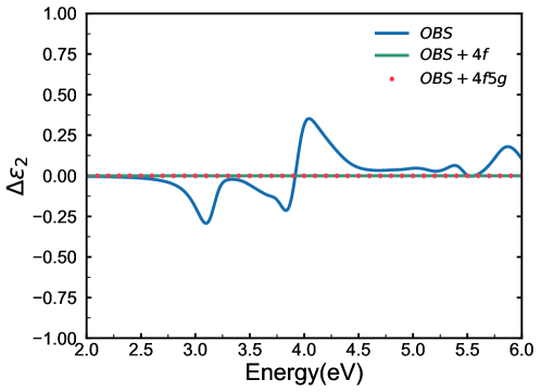
Figure 1: Relative error $\Delta\epsilon_{2}$ of the absorption spectrum of Silicon (Si) from $BSE@G_{0}W_{0}$ calculations under different auxiliary numerical atomic orbitals (NAO) Basis. The standard reference result is performed with the OBS+4f5g6h auxiliary basis. All calculations are performed under $8\times 8\times 8$ $\Gamma$-centered Brillouin zone (BZ) sampling and tier 2 NAO basis set.

4.2 4.2 Convergence of NAO Basis set

In terms of NAO basis sets convergence, a very high precision can be reached in all-electron ground-state Density Functional Theory (DFT) calculations when only occupied KS states need to be evaluated ^{51, 85}. However, similar to the case of Gaussian Type Orbitals (GTOs) and other atom-centered basis sets, the situation becomes more intricate when applied to correlated calculations such as MP2 and RPA. The standard FHI-aims-2009 NAO basis set series (”tier n” basis), while originally designed for ground-state DFT calculations, can also produce accurate results also for MP2 and RPA calculations. ⁴⁹. Enhanced accuracy can be achieved by employing alternative NAO-VCC-$n$Z basis sets ⁸⁶, which allow for results to be extrapolated to the Complete Basis Set (CBS) limit through a two-point extrapolation procedure ⁷². However, it was observed that the original NAO-VCC-$n$Z basis sets, initially designed for molecules, are ill-conditioned for densely packed solids due to their relatively larger radial extent, compared to the tier n basis sets. To address this limitation, Zhang et al. ⁷² optimized these basis sets by eliminating the so-called ’enhanced minimal basis’ and tightening the cutoff radius of the basis functions. The resulting basis sets, referred to as localized NAO-VCC-$n$Z (loc-NAO-VCC-nZ) here, have been demonstrated to yield accurate MP2 and RPA energies for simple solids when used in conjunction with an appropriate extrapolation procedure in Ref. ⁷² To assess basis set convergence, we conducted calculations of the silicon (Si) absorption spectrum using the BSE@$G_{0}W_{0}$ method with two different sets of basis functions: (a) tier n ($n=1,2,3$) and (b) loc-NAO-VCC-$n$Z ($n=2,3,4$). These basis set convergence tests were performed using a $7\times 7\times 7$ $\Gamma$-centered Brillouin zone (BZ) sampling.

As shown in Figure 2 (a), the optical spectrum converges quickly in the tier n basis set, with only a marginal shift in excitation peaks as we increase the basis set size from tier 1 to tier 3. For instance, the energy of the first peak changes by only 0.02 eV from 3.173 eV to 3.149 eV as we move up from tier 1 to tier 3. Conversely, when employing the loc-NAO-VCC-$n$Z basis set, the absorption spectrum for the 2Z basis set is not fully converged as seen in Figure 2 (b). There are indeed some qualitatively incorrect behaviors as evidenced, for example, in the erroneous prediction of multiple peaks around 4 eV as well as the sizable blue-shift of the first excitation at 3.235 eV. These erroneous features can be attributed to the omission of the “enhanced minimal basis” in the loc-NAO-VCC-2Z basis, rendering it insufficient for accurately describing the occupied states in the preceding self-consistent field (SCF) calculations. At the same time, the larger basis sets in this series, loc-NAO-VCC-3Z and loc-NAO-VCC-4Z basis sets, yield converged results, and they also agree well with the converged results using the “tier n” default basis sets of the FHI-aims code. To summarize, with the largest NAO-VCC-4Z and tier 3 basis sets, we achieved a satisfactory agreement within 20 meV for the BSE@$G_{0}W_{0}$ absorption spectrum. We showed here that we can achieve a reliable convergence of the absorption spectrum using atom-centered basis sets like NAO. In the subsequent sections, we employ the default tier 2 basis set of the FHI-aims code as specified in Reference ²⁵.

(a)

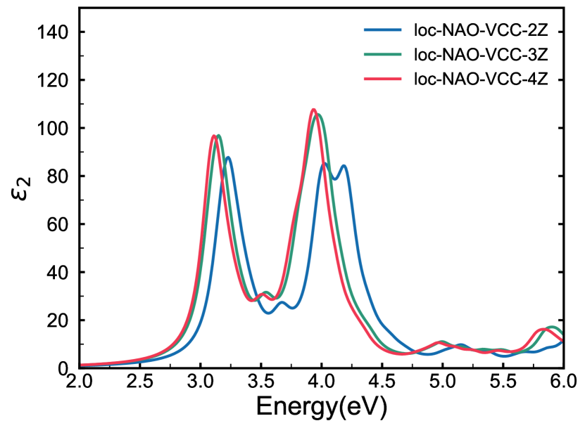
(b)

Figure 2: Convergence of Si absorption spectrum from $BSE@G_{0}W_{0}$ calculation with respect to NAO basis. A Lorentzian broadening of $\eta=0.10eV$ is used. The calculations are performed under $7\times 7\times 7$ $\Gamma$-centered Brillouin zone (BZ) sampling and (a) tier n $(n=1,2,3)$ or (b) loc-NAO-VCC-nZ $(n=2,3,4)$ NAO basis set complemented by the OBS+4f auxiliary NAO basis set.

4.3 4.3 Convergence of Brillouin Zone (BZ) Sampling

One of the most important and also challenging aspects of calculating the optical absorption spectrum of extended condensed matter systems is achieving the convergence with respect to the Brillouin zone (BZ) sampling^{11, 87, 38, 88}. This is a particularly important consideration for many inorganic solids in which there exist strong band dispersion and the band gap is indirect. To accelerate the convergence of the absorption spectrum in BSE calculations, the BZ sampling with a random shifted k-grid around the $\Gamma$ point has been used for practical calculations as discussed in the literature ^{29, 89, 90, 41}. For the purpose of benchmarking our new NAO-based BSE implementation, we do not consider such accelerated k-point sampling techniques in this work, but we focus on the convergence behavior of the direct equally-spaced BZ sampling centered at $\Gamma$ point. To generate quasi-particle (QP) energies for BSE calculation, we employ $G_{0}W_{0}$ calculation for all k-grids instead of applying a consistent scissors shift to Kohn-Sham orbital energies as sometimes performed. In the previous benchmark on the NAO-based $G_{0}W_{0}$ method²⁵, it was found that $7\times 7\times 7$ BZ sampling for the dielectric matrix is adequate to achieve convergence of QP energies within 5 meV.

Figure 3 shows the optical absorption spectrum of crystalline silicon, utilizing $\Gamma$-centered uniform BZ sampling with $n\times n\times n$ where $n=7,10,12,14$. Neither the shape of the absorption spectrum or the excitation energies are converged when employing the $7\times 7\times 7$ BZ sampling, despite the convergence observed for the $G_{0}W_{0}$ QP energies²⁵. With increased BZ samplings, the absorption spectrum generally becomes blue-shifted, particularly for the first absorption peak. At the same time, the peak at around 5.0 eV is seen to red-shift, and the spectrum does not converge uniformly at all energies. In general, the shape of the absorption spectrum tends to converge with the increased BZ sampling from $n=10$ to $n=14$. At the same time, we note that achieving the complete convergence of the absorption spectrum for cystalline silicon, as discussed in Ref. ³⁸, may necessitate an exceedingly fine sampling of the BZ to the value of $n=40$. Unfortunately, our current computational resource limitation does not allow us to achieve the full convergence with such a great BZ sampling at this time. While this present work is focused on demonstration of our new all-electron NAO formalism for BSE@$GW$ method, we will explore incorporating enhanced BZ sampling techniques in our future research effort, such as coarse-grain k-grid interpolation ¹¹, Wannier interpolation ⁸⁷, and other related schemes ^{38, 88}.

Figure 3: Absorption spectrum of Si under $\Gamma$-centered Brillouin zone (BZ) sampling of dimensions $n\times n\times n$ ($n=7,10,12,14$) calculated under tier 2 NAO basis set and OBS+4f auxiliary NAO basis set.A Lorentzian broadening of $\eta=0.15eV$ is used.

4.4 4.4 Comparison with Planewave Basis-Set Result

Having examined the convergence behavior of the BSE calculation for our all-electron NAO based implementation, we now turn to the comparison to the BSE calculation based on the transitional Plane-Wave Pseudopotential (PW-PP) implementation. We performed the PW-PP based BSE@$GW$ calculation using the well-documented codes, the BerkeleyGW package ¹¹. The BSE@$GW$ calculation was performed on top of the DFT calculation using the Quantum Espresso ^{91, 92} code. We used the local density approximation (LDA) to the exchange-correlational functional in the DFT calculation as the starting point⁸⁴. Further details of calculation setting are provided in the Supporting Information.

In Figure 4(a), we present the optical absorption spectrum of crystalline silicon, using a $14\times 14\times 14$ $\Gamma$-centered BZ sampling. Both spectra use the same Lorentzian broadening of 0.15 eV. It is important to note that Contour Deformation (not the widely-used generalized plasma-pole model ⁹³) technique is employed for the numerical (frequency) integration of the self-energy in the $G_{0}W_{0}$ calculation with BerkeleyGW, in order to compare the two methods on an equal footing. Our NAO-based BSE$G_{0}W_{0}$ result closely match the PW-PP result in terms of the peak positions while some differences in the amplitude are observed at around 4.0-5.0 eV. We note that HOMO-LUMO QP energy gap from the $G_{0}W_{0}$ calculations agree very closely between our NAO-based result and the PW-PP result within 6 meV. BSE eigenvalues (i.e. excitation energies) from our NAO-based calculation also closely match with the PW-PP results, exhibiting an average difference of 26 meV.

To better understand the origin of the observed differences in the optical absorption spectrum, Figure 4(b) shows the comparison using the scaled Joint Density of States (JDOS),

$$JDOS(\omega)/\omega^{2}=\frac{16\pi^{2}e^{2}}{\omega^{2}}\sum_{m}\delta(\omega-\omega_{m})$$ (59)

where $\omega_{m}$ is the energy of excited state $m$ from BSE calculation. Instead of having the transition amplitudes convoluted as part of the calculation of the absorption spectrum, the JDOS allows for a direct comparison of electronic transitions as a function of the excitation energy. As seen in Figure 4(b), our NAO-based BSE excitation energies closely align with the PW-PP results, except in the energy range of 4.0-4.5 eV, where a noticeble deviation is observed. This rather small deviation in this energy range has a significant impact on the differences observed in the absorption spectrum as seen in Figure 4(a). Given the fully converged basis set for this particular case of crystalline silicon as discussed above, these differences are attributed to the difference between the all-electron NAO and PW-PP formulations, most likely due to the difference in the frequency integration treatments utilized in the $G_{0}W_{0}$ calculation.

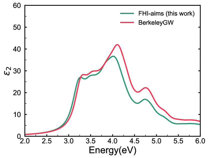
(a)

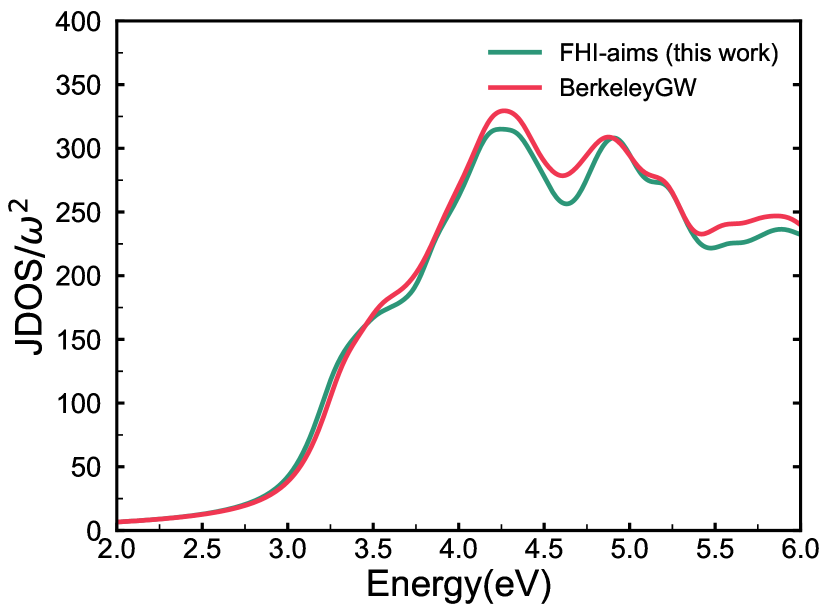
(b)

Figure 4: Comparison of the (a) absorption spectra and (b) Joint density of state (JDOS) divied by $\omega^{2}$ for Si calculation from this implementation in FHI-aims with results from the BerkeleyGW package, performed under a $14\times 14\times 14$ $\Gamma$-centered BZ sampling. A Lorentzian broadening of $\eta=0.15eV$ is used.

5 5. Conclusion

We described the formulation and algorithms of new all-electron periodic BSE implementation within the numeric atom-centered orbital (NAO) framework. To our knowledge, this is the first all-electron NAO-based BSE implementation that works with the periodic boundary conditions. Our implementation was carried out wihtin the FHI-aims code package ^{51, 82}. We use crystalline silicon (Si) as an example to demonstrate our implementation and performed systematic convergence tests with respect to the computational parameters including the NAO basis set size, Auxiliary basis set, and the Brillouin Zone (BZ) sampling. With the fully-converged result in hand, we made a direct comparison of our all-electron NAO result to the obtained using the traditional PW-PP approach implemented BerkeleyGW ¹¹ code with Quantum Espresso ⁸³ code. Though having established the excellent agreement with the well-established implementation of BSE@$GW$ based on the PW-PP formalism, achieving the complete convergence of the optical absorption spectrum may also necessitate an exceedingly fine sampling of the Brillouin zone. ³⁸ Our current implementation supports the standard $\Gamma$-centered sampling. In future research, we will explore incorporating enhanced BZ sampling techniques for BSE calculation, such as coarse-grained k-grid interpolation ¹¹, Wannier interpolation ⁸⁷, and other related methods ^{38, 88}.

6 Acknowledge

We thank the Research Computing at the University of North Carolina at Chapel Hill for computer resources. We thank Jianhang Xu, Minye Zhang and Tianyu Zhu for their helpful discussion.

7 Author Contribution

R.Z. and Y.Y. led and contributed equally to the work. All authors discussed the results and contributed to the final manuscript.

References

- van Setten et al. 2013 van Setten, M. J.; Weigend, F.; Evers, F. The GW-method for quantum chemistry applications: Theory and implementation. Journal of chemical theory and computation 2013, 9, 232–246
- Leng et al. 2016 Leng, X.; Jin, F.; Wei, M.; Ma, Y. GW method and Bethe–Salpeter equation for calculating electronic excitations. Wiley Interdisciplinary Reviews: Computational Molecular Science 2016, 6, 532–550
- Golze et al. 2019 Golze, D.; Dvorak, M.; Rinke, P. The GW compendium: A practical guide to theoretical photoemission spectroscopy. Frontiers in chemistry 2019, 7, 377
- Blase et al. 2020 Blase, X.; Duchemin, I.; Jacquemin, D.; Loos, P.-F. The Bethe–Salpeter equation formalism: From physics to chemistry. The Journal of Physical Chemistry Letters 2020, 11, 7371–7382
- Strinati 1984 Strinati, G. Effects of dynamical screening on resonances at inner-shell thresholds in semiconductors. Physical Review B 1984, 29, 5718
- Albrecht et al. 1998 Albrecht, S.; Reining, L.; Del Sole, R.; Onida, G. Ab initio calculation of excitonic effects in the optical spectra of semiconductors. Physical review letters 1998, 80, 4510
- Rohlfing and Louie 1998 Rohlfing, M.; Louie, S. G. Electron-hole excitations in semiconductors and insulators. Physical review letters 1998, 81, 2312
- Onida et al. 2002 Onida, G.; Reining, L.; Rubio, A. Electronic excitations: density-functional versus many-body Green’s-function approaches. Reviews of modern physics 2002, 74, 601
- Marsili et al. 2017 Marsili, M.; Mosconi, E.; De Angelis, F.; Umari, P. Large-scale G W-BSE calculations with N 3 scaling: Excitonic effects in dye-sensitized solar cells. Physical Review B 2017, 95, 075415
- Vorwerk et al. 2019 Vorwerk, C.; Aurich, B.; Cocchi, C.; Draxl, C. Bethe–Salpeter equation for absorption and scattering spectroscopy: implementation in the exciting code. Electronic Structure 2019, 1, 037001
- Deslippe et al. 2012 Deslippe, J.; Samsonidze, G.; Strubbe, D. A.; Jain, M.; Cohen, M. L.; Louie, S. G. BerkeleyGW: A massively parallel computer package for the calculation of the quasiparticle and optical properties of materials and nanostructures. Computer Physics Communications 2012, 183, 1269–1289
- Faber et al. 2014 Faber, C.; Boulanger, P.; Attaccalite, C.; Duchemin, I.; Blase, X. Excited states properties of organic molecules: From density functional theory to the GW and Bethe–Salpeter Green’s function formalisms. Philosophical Transactions of the Royal Society A: Mathematical, Physical and Engineering Sciences 2014, 372, 20130271
- Jacquemin et al. 2017 Jacquemin, D.; Duchemin, I.; Blase, X. Is the Bethe–Salpeter formalism accurate for excitation energies? Comparisons with TD-DFT, CASPT2, and EOM-CCSD. The journal of physical chemistry letters 2017, 8, 1524–1529
- Blase et al. 2018 Blase, X.; Duchemin, I.; Jacquemin, D. The Bethe–Salpeter equation in chemistry: relations with TD-DFT, applications and challenges. Chemical Society Reviews 2018, 47, 1022–1043
- Casida 1995 Casida, M. E. Recent Advances In Density Functional Methods: (Part I); World Scientific, 1995; pp 155–192
- Ullrich 2011 Ullrich, C. A. Time-dependent density-functional theory: concepts and applications. 2011,
- Bartlett 2012 Bartlett, R. J. Coupled-cluster theory and its equation-of-motion extensions. Wiley Interdisciplinary Reviews: Computational Molecular Science 2012, 2, 126–138
- Krylov 2008 Krylov, A. I. Equation-of-motion coupled-cluster methods for open-shell and electronically excited species: The hitchhiker’s guide to Fock space. Annu. Rev. Phys. Chem. 2008, 59, 433–462
- Yang et al. 2007 Yang, L.; Cohen, M. L.; Louie, S. G. Excitonic effects in the optical spectra of graphene nanoribbons. Nano letters 2007, 7, 3112–3115
- Perebeinos et al. 2005 Perebeinos, V.; Tersoff, J.; Avouris, P. Radiative lifetime of excitons in carbon nanotubes. Nano letters 2005, 5, 2495–2499
- Jacquemin et al. 2015 Jacquemin, D.; Duchemin, I.; Blase, X. Benchmarking the Bethe–Salpeter formalism on a standard organic molecular set. Journal of Chemical Theory and Computation 2015, 11, 3290–3304
- Jacquemin et al. 2016 Jacquemin, D.; Duchemin, I.; Blondel, A.; Blase, X. Assessment of the accuracy of the Bethe–Salpeter (BSE/GW) oscillator strengths. Journal of Chemical Theory and Computation 2016, 12, 3969–3981
- Körbel et al. 2014 Körbel, S.; Boulanger, P.; Duchemin, I.; Blase, X.; Marques, M. A.; Botti, S. Benchmark many-body GW and Bethe–Salpeter calculations for small transition metal molecules. Journal of chemical theory and computation 2014, 10, 3934–3943
- Yao et al. 2022 Yao, Y.; Golze, D.; Rinke, P.; Blum, V.; Kanai, Y. All-electron BSE@ GW method for K-edge core electron excitation energies. Journal of Chemical Theory and Computation 2022, 18, 1569–1583
- Ren et al. 2021 Ren, X.; Merz, F.; Jiang, H.; Yao, Y.; Rampp, M.; Lederer, H.; Blum, V.; Scheffler, M. All-electron periodic G 0 W 0 implementation with numerical atomic orbital basis functions: Algorithm and benchmarks. Physical Review Materials 2021, 5, 013807
- Liu et al. 2020 Liu, C.; Kloppenburg, J.; Yao, Y.; Ren, X.; Appel, H.; Kanai, Y.; Blum, V. All-electron ab initio Bethe-Salpeter equation approach to neutral excitations in molecules with numeric atom-centered orbitals. The Journal of Chemical Physics 2020, 152
- Nakanishi 1969 Nakanishi, N. A general survey of the theory of the Bethe-Salpeter equation. Progress of Theoretical Physics Supplement 1969, 43, 1–81
- Hedin 1965 Hedin, L. New method for calculating the one-particle Green’s function with application to the electron-gas problem. Physical Review 1965, 139, A796
- Rohlfing and Louie 2000 Rohlfing, M.; Louie, S. G. Electron-hole excitations and optical spectra from first principles. Physical Review B 2000, 62, 4927
- Loos and Blase 2020 Loos, P.-F.; Blase, X. Dynamical correction to the Bethe–Salpeter equation beyond the plasmon-pole approximation. The Journal of Chemical Physics 2020, 153
- Zhang et al. 2023 Zhang, X.; Leveillee, J. A.; Schleife, A. Effect of dynamical screening in the Bethe-Salpeter framework: Excitons in crystalline naphthalene. arXiv preprint arXiv:2302.07948 2023,
- Martin et al. 2016 Martin, R. M.; Reining, L.; Ceperley, D. M. Interacting electrons; Cambridge University Press, 2016; pp 345–388
- Shao and Yang 2016 Shao, M.; Yang, C. BSEPACK User’s Guide. arXiv preprint arXiv:1612.07848 2016,
- Benner et al. 2017 Benner, P.; Dolgov, S.; Khoromskaia, V.; Khoromskij, B. N. Fast iterative solution of the Bethe–Salpeter eigenvalue problem using low-rank and QTT tensor approximation. Journal of computational physics 2017, 334, 221–239
- Benner et al. 2018 Benner, P.; Marek, A.; Penke, C. Improving the Performance of Numerical Algorithms for the Bethe-Salpeter Eigenvalue Problem. PAMM 2018, 18, e201800255
- Ljungberg et al. 2015 Ljungberg, M. P.; Koval, P.; Ferrari, F.; Foerster, D.; Sanchez-Portal, D. Cubic-scaling iterative solution of the Bethe-Salpeter equation for finite systems. Physical Review B 2015, 92, 075422
- Rocca et al. 2014 Rocca, D.; Vörös, M.; Gali, A.; Galli, G. Ab initio optoelectronic properties of silicon nanoparticles: Excitation energies, sum rules, and Tamm–Dancoff approximation. Journal of Chemical Theory and Computation 2014, 10, 3290–3298
- Sander et al. 2015 Sander, T.; Maggio, E.; Kresse, G. Beyond the Tamm-Dancoff approximation for extended systems using exact diagonalization. Physical Review B 2015, 92, 045209
- Hirata and Head-Gordon 1999 Hirata, S.; Head-Gordon, M. Time-dependent density functional theory within the Tamm–Dancoff approximation. Chemical Physics Letters 1999, 314, 291–299
- Chantzis et al. 2013 Chantzis, A.; Laurent, A. D.; Adamo, C.; Jacquemin, D. Is the Tamm-Dancoff approximation reliable for the calculation of absorption and fluorescence band shapes? Journal of chemical theory and computation 2013, 9, 4517–4525
- Rocca et al. 2012 Rocca, D.; Ping, Y.; Gebauer, R.; Galli, G. Solution of the Bethe-Salpeter equation without empty electronic states: Application to the absorption spectra of bulk systems. Physical Review B 2012, 85, 045116
- Blase et al. 2011 Blase, X.; Attaccalite, C.; Olevano, V. First-principles GW calculations for fullerenes, porphyrins, phtalocyanine, and other molecules of interest for organic photovoltaic applications. Physical Review B 2011, 83, 115103
- Faber et al. 2012 Faber, C.; Duchemin, I.; Deutsch, T.; Attaccalite, C.; Olevano, V.; Blase, X. Electron–phonon coupling and charge-transfer excitations in organic systems from many-body perturbation theory: The Fiesta code, an efficient Gaussian-basis implementation of the GW and Bethe–Salpeter formalisms. Journal of Materials Science 2012, 47, 7472–7481
- Wilhelm et al. 2016 Wilhelm, J.; Del Ben, M.; Hutter, J. GW in the Gaussian and plane waves scheme with application to linear acenes. Journal of Chemical Theory and Computation 2016, 12, 3623–3635
- Wilhelm and Hutter 2017 Wilhelm, J.; Hutter, J. Periodic G W calculations in the Gaussian and plane-waves scheme. Physical Review B 2017, 95, 235123
- Bruneval et al. 2016 Bruneval, F.; Rangel, T.; Hamed, S. M.; Shao, M.; Yang, C.; Neaton, J. B. molgw 1: Many-body perturbation theory software for atoms, molecules, and clusters. Computer Physics Communications 2016, 208, 149–161
- Zhu and Chan 2021 Zhu, T.; Chan, G. K.-L. All-electron Gaussian-based G 0 W 0 for valence and core excitation energies of periodic systems. Journal of Chemical Theory and Computation 2021, 17, 727–741
- Lei and Zhu 2022 Lei, J.; Zhu, T. Gaussian-based quasiparticle self-consistent GW for periodic systems. The Journal of Chemical Physics 2022, 157
- Ren et al. 2012 Ren, X.; Rinke, P.; Blum, V.; Wieferink, J.; Tkatchenko, A.; Sanfilippo, A.; Reuter, K.; Scheffler, M. Resolution-of-identity approach to Hartree–Fock, hybrid density functionals, RPA, MP2 and GW with numeric atom-centered orbital basis functions. New Journal of Physics 2012, 14, 053020
- Bruneval et al. 2015 Bruneval, F.; Hamed, S. M.; Neaton, J. B. A systematic benchmark of the ab initio Bethe-Salpeter equation approach for low-lying optical excitations of small organic molecules. The Journal of Chemical Physics 2015, 142
- Blum et al. 2009 Blum, V.; Gehrke, R.; Hanke, F.; Havu, P.; Havu, V.; Ren, X.; Reuter, K.; Scheffler, M. Ab initio molecular simulations with numeric atom-centered orbitals. Computer Physics Communications 2009, 180, 2175–2196
- Szabo and Ostlund 2012 Szabo, A.; Ostlund, N. S. Modern quantum chemistry: introduction to advanced electronic structure theory; Courier Corporation, 2012
- Whitten 1973 Whitten, J. L. Coulombic potential energy integrals and approximations. The Journal of Chemical Physics 1973, 58, 4496–4501
- Dunlap et al. 1979 Dunlap, B. I.; Connolly, J.; Sabin, J. On some approximations in applications of X theory. The Journal of Chemical Physics 1979, 71, 3396–3402
- Vahtras et al. 1993 Vahtras, O.; Almlöf, J.; Feyereisen, M. Integral approximations for LCAO-SCF calculations. Chemical Physics Letters 1993, 213, 514–518
- Weigend 2002 Weigend, F. A fully direct RI-HF algorithm: Implementation, optimised auxiliary basis sets, demonstration of accuracy and efficiency. Physical Chemistry Chemical Physics 2002, 4, 4285–4291
- Feyereisen et al. 1993 Feyereisen, M.; Fitzgerald, G.; Komornicki, A. Use of approximate integrals in ab initio theory. An application in MP2 energy calculations. Chemical physics letters 1993, 208, 359–363
- Weigend et al. 1998 Weigend, F.; Häser, M.; Patzelt, H.; Ahlrichs, R. RI-MP2: optimized auxiliary basis sets and demonstration of efficiency. Chemical physics letters 1998, 294, 143–152
- Hättig 2003 Hättig, C. Geometry optimizations with the coupled-cluster model CC2 using the resolution-of-the-identity approximation. The Journal of chemical physics 2003, 118, 7751–7761
- Schütz and Manby 2003 Schütz, M.; Manby, F. R. Linear scaling local coupled cluster theory with density fitting. Part I: 4-external integrals. Physical Chemistry Chemical Physics 2003, 5, 3349–3358
- Sierka et al. 2003 Sierka, M.; Hogekamp, A.; Ahlrichs, R. Fast evaluation of the Coulomb potential for electron densities using multipole accelerated resolution of identity approximation. The Journal of chemical physics 2003, 118, 9136–9148
- Bloch 1929 Bloch, F. Über die quantenmechanik der elektronen in kristallgittern. Zeitschrift für physik 1929, 52, 555–600
- Adler 1962 Adler, S. L. Quantum theory of the dielectric constant in real solids. Physical Review 1962, 126, 413
- Wiser 1963 Wiser, N. Dielectric constant with local field effects included. Physical Review 1963, 129, 62
- Sun et al. 2017 Sun, Q.; Berkelbach, T. C.; McClain, J. D.; Chan, G. K. Gaussian and plane-wave mixed density fitting for periodic systems. The Journal of chemical physics 2017, 147
- Ye and Berkelbach 2021 Ye, H.-Z.; Berkelbach, T. C. Fast periodic Gaussian density fitting by range separation. The Journal of Chemical Physics 2021, 154
- Ihrig et al. 2015 Ihrig, A. C.; Wieferink, J.; Zhang, I. Y.; Ropo, M.; Ren, X.; Rinke, P.; Scheffler, M.; Blum, V. Accurate localized resolution of identity approach for linear-scaling hybrid density functionals and for many-body perturbation theory. New Journal of Physics 2015, 17, 093020
- Merlot et al. 2013 Merlot, P.; Kjærgaard, T.; Helgaker, T.; Lindh, R.; Aquilante, F.; Reine, S.; Pedersen, T. B. Attractive electron–electron interactions within robust local fitting approximations. Journal of Computational Chemistry 2013, 34, 1486–1496
- Wirz et al. 2017 Wirz, L. N.; Reine, S. S.; Pedersen, T. B. On resolution-of-the-identity electron repulsion integral approximations and variational stability. Journal of Chemical Theory and Computation 2017, 13, 4897–4906
- Levchenko et al. 2015 Levchenko, S. V.; Ren, X.; Wieferink, J.; Johanni, R.; Rinke, P.; Blum, V.; Scheffler, M. Hybrid functionals for large periodic systems in an all-electron, numeric atom-centered basis framework. Computer Physics Communications 2015, 192, 60–69
- Lin et al. 2020 Lin, P.; Ren, X.; He, L. Accuracy of localized resolution of the identity in periodic hybrid functional calculations with numerical atomic orbitals. The Journal of Physical Chemistry Letters 2020, 11, 3082–3088
- Zhang et al. 2019 Zhang, I. Y.; Logsdail, A. J.; Ren, X.; Levchenko, S. V.; Ghiringhelli, L.; Scheffler, M. Main-group test set for materials science and engineering with user-friendly graphical tools for error analysis: systematic benchmark of the numerical and intrinsic errors in state-of-the-art electronic-structure approximations. New Journal of Physics 2019, 21, 013025
- Shi et al. 2024 Shi, R.; Lin, P.; Zhang, M.-Y.; He, L.; Ren, X. Subquadratic-scaling real-space random phase approximation correlation energy calculations for periodic systems with numerical atomic orbitals. Physical Review B 2024, 109, 035103
- Gygi and Baldereschi 1986 Gygi, F.; Baldereschi, A. Self-consistent Hartree-Fock and screened-exchange calculations in solids: Application to silicon. Physical Review B 1986, 34, 4405
- Spencer and Alavi 2008 Spencer, J.; Alavi, A. Efficient calculation of the exact exchange energy in periodic systems using a truncated Coulomb potential. Physical Review B 2008, 77, 193110
- Massidda et al. 1993 Massidda, S.; Posternak, M.; Baldereschi, A. Hartree-Fock LAPW approach to the electronic properties of periodic systems. Physical Review B 1993, 48, 5058
- Hüser et al. 2013 Hüser, F.; Olsen, T.; Thygesen, K. S. Quasiparticle GW calculations for solids, molecules, and two-dimensional materials. Physical Review B 2013, 87, 235132
- Jiang et al. 2013 Jiang, H.; Gómez-Abal, R. I.; Li, X.-Z.; Meisenbichler, C.; Ambrosch-Draxl, C.; Scheffler, M. FHI-gap: A GW code based on the all-electron augmented plane wave method. Computer Physics Communications 2013, 184, 348–366
- Ping et al. 2013 Ping, Y.; Rocca, D.; Galli, G. Electronic excitations in light absorbers for photoelectrochemical energy conversion: first principles calculations based on many body perturbation theory. Chemical Society Reviews 2013, 42, 2437–2469
- Friedrich et al. 2009 Friedrich, C.; Schindlmayr, A.; Blügel, S. Efficient calculation of the Coulomb matrix and its expansion around k= 0 within the FLAPW method. Computer physics communications 2009, 180, 347–359
- Friedrich et al. 2010 Friedrich, C.; Blügel, S.; Schindlmayr, A. Efficient implementation of the G W approximation within the all-electron FLAPW method. Physical Review B 2010, 81, 125102
- Blum et al. 2022 Blum, V.; Rossi, M.; Kokott, S.; Scheffler, M. The FHI-aims Code: All-electron, ab initio materials simulations towards the exascale. arXiv preprint arXiv:2208.12335 2022,
- Giannozzi et al. 2020 Giannozzi, P.; Baseggio, O.; Bonfà, P.; Brunato, D.; Car, R.; Carnimeo, I.; Cavazzoni, C.; De Gironcoli, S.; Delugas, P.; Ferrari Ruffino, F.; others Quantum ESPRESSO toward the exascale. The Journal of chemical physics 2020, 152
- Perdew and Wang 1992 Perdew, J. P.; Wang, Y. Accurate and simple analytic representation of the electron-gas correlation energy. Physical review B 1992, 45, 13244
- Jensen et al. 2017 Jensen, S. R.; Saha, S.; Flores-Livas, J. A.; Huhn, W.; Blum, V.; Goedecker, S.; Frediani, L. The elephant in the room of density functional theory calculations. The journal of physical chemistry letters 2017, 8, 1449–1457
- Zhang et al. 2013 Zhang, I. Y.; Ren, X.; Rinke, P.; Blum, V.; Scheffler, M. Numeric atom-centered-orbital basis sets with valence-correlation consistency from H to Ar. New Journal of Physics 2013, 15, 123033
- Kammerlander et al. 2012 Kammerlander, D.; Botti, S.; Marques, M. A.; Marini, A.; Attaccalite, C. Speeding up the solution of the Bethe-Salpeter equation by a double-grid method and Wannier interpolation. Physical Review B 2012, 86, 125203
- Gillet et al. 2016 Gillet, Y.; Giantomassi, M.; Gonze, X. Efficient on-the-fly interpolation technique for Bethe–Salpeter calculations of optical spectra. Computer Physics Communications 2016, 203, 83–93
- Schmidt et al. 2003 Schmidt, W.; Glutsch, S.; Hahn, P.; Bechstedt, F. Efficient O (N 2) method to solve the Bethe-Salpeter equation. Physical Review B 2003, 67, 085307
- Marini et al. 2009 Marini, A.; Hogan, C.; Grüning, M.; Varsano, D. Yambo: an ab initio tool for excited state calculations. Computer Physics Communications 2009, 180, 1392–1403
- Giannozzi et al. 2009 Giannozzi, P.; Baroni, S.; Bonini, N.; Calandra, M.; Car, R.; Cavazzoni, C.; Ceresoli, D.; Chiarotti, G. L.; Cococcioni, M.; Dabo, I.; others QUANTUM ESPRESSO: a modular and open-source software project for quantum simulations of materials. Journal of physics: Condensed matter 2009, 21, 395502
- Giannozzi et al. 2017 Giannozzi, P.; Andreussi, O.; Brumme, T.; Bunau, O.; Nardelli, M. B.; Calandra, M.; Car, R.; Cavazzoni, C.; Ceresoli, D.; Cococcioni, M.; others Advanced capabilities for materials modelling with Quantum ESPRESSO. Journal of physics: Condensed matter 2017, 29, 465901
- Hybertsen and Louie 1986 Hybertsen, M. S.; Louie, S. G. Electron correlation in semiconductors and insulators: Band gaps and quasiparticle energies. Physical Review B 1986, 34, 5390