Spanwise wall forcing can reduce turbulent heat transfer more than drag

Abstract

Direct numerical simulations are performed of turbulent forced convection in a channel flow with spanwise wall oscillation, either as a plane oscillation or as a streamwise travelling wave. The friction Reynolds number is fixed at $Re_{\tau_{0}}=590$, but the Prandtl number $Pr$ is varied from 0.71 to 20. For $Pr>1$, the heat transfer is reduced by more than the drag, 40% compared to 30% at $Pr=7.5$. This Reynolds analogy breaking is related to the different responses of the velocity and thermal fields to the Stokes layer. It is shown that the Stokes layer near the wall attenuates the large-scale energy of the turbulent heat-flux and the turbulent shear-stress, but amplifies their small-scale energy. At higher Prandtl numbers, the thinning of the conductive sublayer means that the energetic scales of the turbulent heat-flux move closer to the wall, where they are exposed to a stronger Stokes layer production, increasing the contribution of the small-scale energy amplification. A predictive model is derived for the Reynolds and Prandtl number dependence of the heat-transfer reduction based on the scaling of the thermal statistics. The model agrees well with the computations for Prandtl numbers up to 20.

1 Introduction

In many industrial applications, controlling heat transfer is as important as controlling drag. Some examples of the kinds of methods to control both drag and heat transfer are given in figure 1. The performance of any given method is commonly based on the changes achieved in the skin-friction coefficient $C_{f}$ and the Stanton number $C_{h}$, where

$$C_{f}\equiv\frac{2\overline{\tau_{w}}}{\rho U_{\mathrm{ref}}^{2}},\quad C_{h}\equiv\frac{\overline{q_{w}}}{\rho c_{p}U_{\mathrm{ref}}(T_{w}-T_{\mathrm{ref}})}.$$ (1)

Here $\overline{\tau_{w}}$, $\overline{q_{w}}$, $\rho$, $c_{p}$ and $T_{w}$ are the wall shear-stress, wall heat-flux, fluid density, its specific heat capacity and wall temperature, respectively. In a boundary layer, $U_{\mathrm{ref}}$ and $T_{\mathrm{ref}}$ are the free-stream velocity and temperature (Walsh & Weinstein, 1979), and in a channel flow, $U_{\mathrm{ref}}$ and $T_{\mathrm{ref}}$ are the bulk velocity and either the bulk temperature (Stalio & Nobile, 2003) or the mixed-mean temperature (Dipprey & Sabersky, 1963; MacDonald et al., 2019; Rouhi et al., 2022).

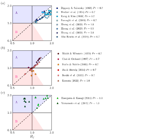
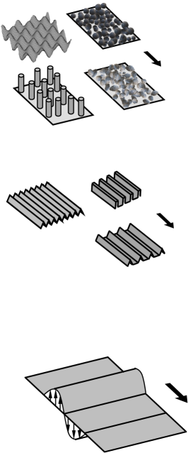
Figure 1: Performance plots showing the fractional changes in the skin-friction coefficient $R_{f}=C_{f}/C_{f_{0}}$ and Stanton number $R_{h}=C_{h}/C_{h_{0}}$ (log-log scale). The diagonal dashed line represents the Reynolds analogy line. (a) Grit or irregular roughness (Dipprey & Sabersky, 1963; Forooghi et al., 2018), spherical roughness (Healzer et al., 1974), pin fins (Kang & Kim, 1999) and egg-carton roughness (Zhong et al., 2023; Rowin et al., 2024). (b) Riblets (Walsh & Weinstein, 1979; Choi & Orchard, 1997; Stalio & Nobile, 2003; Jin & Herwig, 2014; Rouhi et al., 2022; Kuwata, 2022). (c) Wall blowing/suction (Hasegawa & Kasagi, 2011; Yamamoto et al., 2013).

Figure 1 also shows the type of performance plot that is often used to measure the efficacy of control methods (Fan et al., 2009; Bunker, 2013; Huang et al., 2017; Rouhi et al., 2022). Here $C_{f}$ and $C_{h}$ are measured in the flow with control (the target case), and $C_{f_{0}}$ and $C_{h_{0}}$ are measured in the absence of control (the reference case), at matched Reynolds and Prandtl numbers. The diagonal dashed-line represents the Reynolds analogy line, that is, where the fractional change in drag $R_{f}$ ($=C_{f}/C_{f_{0}}$) is equal to the fractional change in heat transfer $R_{h}$ ($=C_{h}/C_{h_{0}}$). Whenever the target case departs from the dashed-line, it breaks the Reynolds analogy. Type A applications (shaded in purple) demand heat-transfer augmentation with the minimum pumping power, hence minimum drag. Examples include cooling passages of gas turbine blades (Baek et al., 2022; Otto et al., 2022) and solar air collectors (Vengadesan & Senthil, 2020). Type B applications (shaded in pink) demand heat-transfer reduction with the minimum pumping power, e.g. crude oil transportation (Yu et al., 2010; Han et al., 2015; Yuan et al., 2023) or heat energy transportation (Ma et al., 2009; Xie & Jiang, 2017). In such applications, the fluid is heated to reduce its viscosity and decrease the friction loss, and the heat loss needs to be minimised to maintain efficiency.

From figure 1(a), we see that rough surfaces and pin fins augment the heat transfer ($R_{h}>1$), but for most data points the drag increase exceeds the heat-transfer increase ($R_{f}>R_{h}>1$), and so they fall outside the objective space for either type A or B applications. Yamamoto et al. (2013) and Rouhi et al. (2022) relate such performance to the pressure drag. For surface protrusions like roughness, viscous drag and pressure drag both contribute to $C_{f}$. However, $C_{h}$ consists of the wall heat-flux only, which is the analogue of the viscous drag (MacDonald et al., 2019). Therefore, $C_{f}$ has an additional positive component (pressure drag) compared to $C_{h}$, leading to $R_{f}>R_{h}$.

In figure 1(b), we show the performance of riblets, as two-dimensional streamwise-aligned surface protrusions which do not induce pressure drag. Most data points are scattered near the Reynolds analogy line, but a few data points break the analogy towards the regions for type A or B applications. Rouhi et al. (2022) and Kuwata (2022) relate such behaviour to the formation of Kelvin-Helmholtz rollers and secondary flows by certain riblet designs.

Figure 1(c) shows the data for wall blowing/suction. Compared to roughness and riblets, wall blowing/suction breaks the Reynolds analogy to a higher degree towards the objective space for type A applications. In particular, the data points of Yamamoto et al. (2013) yield simultaneous heat-transfer augmentation and drag reduction ($R_{h}>1>R_{f}$). They relate this performance to the formation of spanwise-aligned coherent motions.

In the present study, we focus on spanwise wall oscillation described by

$$W_{s}(x,t)=A\sin(\kappa_{x}x+\omega t)$$ (2)

where $W_{s}$ is the instantaneous spanwise surface velocity that oscillates with amplitude $A$ and frequency $\omega$. With $\kappa_{x}\neq 0$, the mechanism generates a streamwise travelling wave, and with $\kappa_{x}=0$ the motion is a simple spanwise oscillating plane (as illustrated in figure 2). The drag performance of (2) has been extensively investigated in the literature (Jung et al., 1992; Quadrio & Sibilla, 2000; Quadrio et al., 2009; Viotti et al., 2009; Quadrio & Ricco, 2011; Quadrio, 2011; Gatti & Quadrio, 2013; Hurst et al., 2014; Gatti & Quadrio, 2016; Marusic et al., 2021; Rouhi et al., 2023; Chandran et al., 2023). With the optimal combination of $A$, $\kappa_{x}$, and $\omega$, wall oscillations can reduce drag by $40\%$. However, there are only a few studies on the performance of (2) in controlling turbulent heat-transfer (Fang et al., 2009, 2010; Guérin et al., 2023). In figure 2(a), we overlay the DNS data point of Guérin et al. (2023) for spanwise plane oscillation ($\kappa_{x}=0$) of turbulent channel flow at $Re_{\tau_{0}}=180$ and $Pr=1.0$. Here, $Re_{\tau_{0}}=hu_{\tau_{0}}/\nu$, where $h$ is the channel half height, $u_{\tau_{0}}=\sqrt{\overline{\tau_{w_{0}}}/\rho}$, and $\nu$ is the fluid kinematic viscosity. By operating at a large viscous-scaled actuation period ($T^{+}_{osc}=2\pi/\omega^{+}=2\pi u^{2}_{\tau_{0}}/(\omega\nu)=500$) and a large amplitude of oscillation ($A^{+}=A/u_{\tau_{0}}=30$), the drag increased by $7.7\%$ ($R_{f}=1.077$) while the heat transfer increased by $15\%$ ($R_{h}=1.15$), so that this case falls into the objective space for type A applications. The superscript ‘$+$’ indicates normalisation using the viscous length ($\nu/u_{\tau_{0}}$) and velocity ($u_{\tau_{0}}$) scales. The superscript ‘$\ast$’ indicates viscous scaling based on the actual friction velocity, that is, $u_{\tau}$ of the drag-altered flow for the actuated cases.

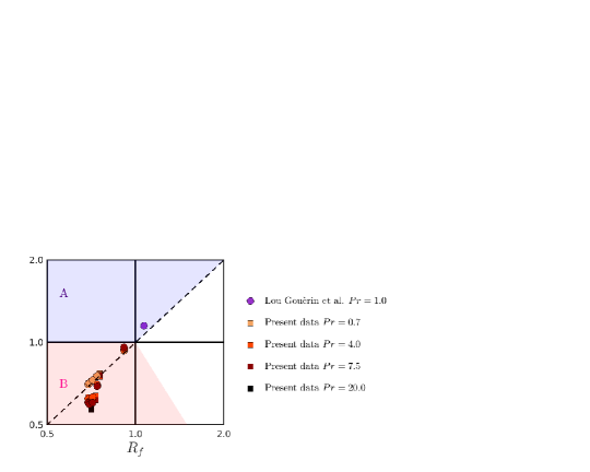
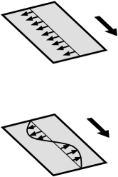
Figure 2: Performance plot similar to figure 1, but for the spanwise wall oscillation via streamwise travelling wave (square symbols, $\kappa_{x}\neq 0$ in 2) or plane oscillation (circle symbols, $\kappa_{x}=0$ in 2); the purple data point corresponds to the study of Guérin et al. (2023), and the rest of the data points correspond to our present study (table 1). For the present data, the colour of data points becomes darker by increasing $Pr$.

Here, we investigate the effects of spanwise wall oscillation (2) on drag and heat transfer by conducting DNS of turbulent forced convection in a channel flow at $Re_{\tau_{0}}=590$ (figure 2 and table 1). We consider two possible motions: plane oscillations and upstream travelling waves where $\omega>0$. Dimensional analysis for the drag yields

$$R_{f}=C_{f}/C_{f_{0}}=f_{f}(A^{+},\kappa^{+}_{x},\omega^{+},Re_{\tau_{0}})$$ (3)

(Marusic et al., 2021; Rouhi et al., 2023). For the heat transfer, we need to include the Prandtl number $Pr=\nu/\alpha$, where $\alpha$ is the fluid thermal diffusivity, and we find

$$R_{h}=C_{h}/C_{h_{0}}=f_{h}(A^{+},\kappa^{+}_{x},\omega^{+},Re_{\tau_{0}},Pr).$$ (4)

The drag reduction is given by $DR=1-R_{f}$, and the heat-transfer reduction is given by $HR=1-R_{h}$. We vary $Pr$ to assess the performance of (2) in different fluids, including air ($Pr=0.71$), water ($Pr=7.5$) and molten salt ($Pr=20.0$). We fix $A^{+}=12$ and consider the viscous-scaled actuation wavenumbers $\kappa^{+}_{x}=0$ (plane oscillation) and $0.0014$ (travelling wave, $\lambda^{+}\simeq 4500$), indicated respectively with filled circles and squares in figure 2. We vary $\omega^{+}$ from $0.022$ to $0.110$, corresponding to the regime where we expect significant drag reduction (Quadrio et al., 2009; Gatti & Quadrio, 2016; Rouhi et al., 2023). These actuation parameters fall within the inner-scaled actuation pathway ($T^{+}_{osc}\lesssim 350\rightarrow\omega^{+}\gtrsim 0.018$), where $DR$ and $HR$ are achieved through attenuation of the near-wall turbulence in the inner region (Marusic et al., 2021). Our preference for the present actuation parameters is motivated by an existing surface-actuation test bed (Marusic et al., 2021; Chandran et al., 2023), that can operate under these conditions. This provides the opportunity to extend the present numerical study through experiment.

As an overview, we note that all our results give a decrease in drag and heat transfer, with maximum $DR=30\%$ and $HR=40\%$ (see figure 2). For Prandtl numbers greater than one, however, $HR$ increases more than $DR$, breaking the Reynolds analogy. The results fall into the objective space for type B applications (see figure 1), a space that has largely been neglected in the past despite its industrial relevance. In §3.5, we derive a model that predicts that the mechanism can reduce the heat loss beyond $50\%$ for $Pr\gtrsim\mathcal{O}(10^{2})$, a regime that is important for crude oil transportation through pipelines. Our model is supported by our DNS data point at $Pr=20$ that yields $HR=43\%$ (black square in figure 2). We also discover that the Stokes layer, formed in close proximity to the wall in response to the wall oscillation, is the key mechanism that distorts the near-wall temperature field differently than the velocity field when $Pr>1$, leading to $HR>DR$.

2 Numerical flow setup

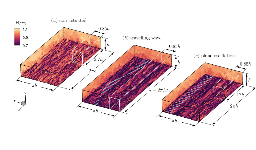
Figure 3: Computational configurations and their domain sizes in the present study. (a) Non-actuated channel flow as the reference. (b) actuated channel flow with the travelling wave with $A^{+}=12$, $\kappa^{+}_{x}=0.0014$; the domain length encompasses one wavelength $L_{x}=2\pi/\kappa_{x}\simeq 7.6h$. (c) Actuated channel flow with spanwise plane oscillation with $A^{+}=12$. In (b,c), we overlay the instantaneous wall motion as a vector field. Full domain shown by the large box with black edges; reduced domain shown by the small box with white edges. In (a,b,c), we visualise the instantaneous fields of $\Theta$ at $y^{+}=15,Re_{\tau_{0}}=590$ and $Pr=7.5$, and for $\omega^{+}=0.088$ in (b,c).

2.1 Governing equations and simulation setup

The governing equations for an incompressible fluid with constant $\rho,\nu$ and thermal diffusivity $\alpha$ are solved in a channel flow (figure 3), where

$$\bm{\nabla}\bm{\cdot}\mathbf{U} = 0,$$ (5)

$$\frac{\partial\mathbf{U}}{\partial t}+\bm{\nabla}\bm{\cdot}\mathbf{(UU)} = -\frac{1}{\rho}\bm{\nabla}p+\nu\nabla^{2}\mathbf{U}-\frac{1}{\rho}\frac{\mathrm{d}\overline{P}}{\mathrm{d}x}\hat{\mathbf{e}}_{x},$$ (6)

$$\frac{\partial\Theta}{\partial t}+\bm{\nabla}\bm{\cdot}(\mathbf{U}\Theta) = \alpha\nabla^{2}\Theta-U\frac{\mathrm{d}T_{w}}{\mathrm{d}x},$$ (7)

and (5), (6) and (7) are the continuity, velocity and temperature transport equations, respectively. We ignore buoyancy, as appropriate for forced convection. In our notation, $\mathbf{U}=(U,V,W)$ is the velocity vector, and $x$, $y$ and $z$ are the streamwise, wall-normal and spanwise directions, respectively. In (6), the total pressure gradient was decomposed into the driving (mean) part $\mathrm{d}\overline{P}/\mathrm{d}x$ and the periodic part $\bm{\nabla}p$. Similarly, the total temperature $T=(dT_{w}/dx)x+\Theta$ was decomposed into the mean part $dT_{w}/dx$ and the periodic part $\Theta$. This thermal driving approach imposes a prescribed mean heat flux at the wall, making it a suitable boundary condition for a periodic domain, and it has been widely used for the simulation of forced convection in a channel flow (Kasagi et al., 1992; Watanabe & Takahashi, 2002; Stalio & Nobile, 2003; Jin & Herwig, 2014; Alcántara-Ávila & Hoyas, 2021; Alcántara-Ávila et al., 2021; Rouhi et al., 2022). By averaging (6) and (7) in time and over the entire fluid domain, we obtain

$$-\frac{1}{\rho}\frac{\mathrm{d}\overline{P}}{\mathrm{d}x}h=\frac{\overline{\tau_{w}}}{\rho}\equiv u^{2}_{\tau},\qquad-U_{b}\frac{\mathrm{d}T_{w}}{\mathrm{d}x}h=\frac{\overline{q_{w}}}{\rho c_{p}}\equiv\theta_{\tau}u_{\tau}$$ (2.4a,b)

where $\overline{\tau_{w}}$ and $\overline{q_{w}}$ are respectively the $xz$-plane and time averaged wall shear-stress and wall heat-flux, $U_{b}$ is the bulk velocity, $h$ is the channel height, $u_{\tau}$ and $\theta_{\tau}$ are the friction velocity and friction temperature, and $c_{p}$ is the specific heat capacity. We adjust $d\overline{P}/dx$ based on a target flow rate (namely, a bulk Reynolds number $Re_{b}\equiv U_{b}h/\nu$) that is matched between the non-actuated reference case (figure 3a) and the actuated cases (figure 3b,c).

Equations (5-7) are solved using a fully conservative fourth-order finite difference code, employed by previous DNS studies of thermal convection (Ng et al., 2015; Rouhi et al., 2021; Zhong et al., 2023; Rowin et al., 2024). The channel flow has periodic boundary conditions in the streamwise and spanwise directions (figure 3). The bottom-wall velocity boundary conditions are $U=V=W=0$ for the non-actuated channel flow (figure 3a), $U=V=0$, $W=A\sin(\kappa_{x}x+\omega t)$ for the actuated channel flow with the travelling wave (figure 3b), and $U=V=0$, $W=A\sin(\omega t)$ for the actuated channel flow with the spanwise plane oscillation (figure 3c). The top boundary conditions for the velocity are the free-slip and impermeable conditions $(\partial U/\partial y=\partial W/\partial y=V=0)$. The boundary conditions for $\Theta$ at the bottom wall and top boundary are $\Theta=0$ and $\partial\Theta/\partial y=0$, respectively. In other words, the total temperature at the bottom wall increases linearly in the $x$-direction $T=(dT_{w}/dx)x$, and at the top boundary the boundary condition is adiabatic ($\partial T/\partial y=0$).

Throughout this manuscript, we call $\Theta$ the temperature. We denote the $xz$-plane and time averaged quantities with overbars (e.g. $\overline{\Theta}$ is the plane and time averaged $\Theta$), the turbulent quantities with lowercase letters (e.g. $\theta$ is the turbulent temperature). Following this notation, $\overline{u^{2}}$ and $\overline{uv}$ are the turbulent stress components, and $\overline{\theta^{2}}$ and $\overline{\theta v}$ are their analogue for the turbulent temperature fluxes.

2.2 Simulation cases

Table 1 summarises the production calculations. All the calculations were performed at a fixed bulk Reynolds number $Re_{b}\simeq 11004$, equivalent to a friction Reynolds number $Re_{\tau_{0}}=590$ for the non-actuated flow. The streamwise and spanwise grid sizes are $\Delta^{+}_{x}\times\Delta^{+}_{z}\simeq 8\times 4$, chosen based on extensive validation studies, as described in Appendix A. In comparison, Alcántara-Ávila & Hoyas (2021) used $\Delta^{+}_{x}\times\Delta^{+}_{z}\simeq 8\times 4$ for turbulent channel flow at $Re_{\tau_{0}}=500$ and $1\leq Pr\leq 7$, while Pirozzoli (2023) used $\Delta^{+}_{x}\times\Delta^{+}_{z}\simeq 10\times 4.5$ for turbulent pipe flow at $Re_{\tau_{0}}\simeq 1100$ and $Pr\leq 16$. As shown in Appendix A, we obtain less than $2\%$ difference in $DR$ and $HR$ when using finer resolutions than $\Delta^{+}_{x}\times\Delta^{+}_{z}\simeq 8\times 4$ (tables 2 to 4), and find very good agreement in the first and second order temperature statistics as well as the spectrograms (figures 22 to 24).

non-actuated		travelling wave			oscillating plane
		$A^{+}=12,\kappa^{+}_{x}=0.0014$			$A^{+}=12$
$L_{x},L_{z}$	$\Delta^{+}_{x},\Delta^{+}_{z}$	$\omega^{+}$	$L_{x},L_{z}$	$\Delta^{+}_{x},\Delta^{+}_{z}$	$\omega^{+}$	$L_{x},L_{z}$	$\Delta^{+}_{x},\Delta^{+}_{z}$
$2.7h,0.85h$	$8.3,3.9$	$0.022$	$7.6h,0.85h$	$8.8,3.9$	$0.022$	$2.7h,0.85h$	$8.3,3.9$
		$0.044$	$7.6h,0.85h$	$8.8,3.9$	$0.044$	$2.7h,0.85h$	$8.3,3.9$
		$0.066$	$7.6h,0.85h$	$8.8,3.9$	$0.066$	$2.7h,0.85h$	$8.3,3.9$	$Pr=0.71$
		$0.088$	$7.6h,0.85h$	$8.8,3.9$	$0.088$	$2.7h,0.85h$	$8.3,3.9$
		$0.110$	$7.6h,0.85h$	$8.8,3.9$	$0.110$	$2.7h,0.85h$	$8.3,3.9$
$2.7h,0.85h$	$8.3,3.9$	$0.022$	$7.6h,0.85h$	$8.8,3.9$	$0.022$	$2.7h,0.85h$	$8.3,3.9$
		$0.044$	$7.6h,0.85h$	$8.8,3.9$	$0.044$	$2.7h,0.85h$	$8.3,3.9$
		$0.066$	$7.6h,0.85h$	$8.8,3.9$	$0.066$	$2.7h,0.85h$	$8.3,3.9$	$Pr=4.0$
		$0.088$	$7.6h,0.85h$	$8.8,3.9$	$0.088$	$2.7h,0.85h$	$8.3,3.9$
		$0.110$	$7.6h,0.85h$	$8.8,3.9$	$0.110$	$2.7h,0.85h$	$8.3,3.9$
$2.7h,0.85h$	$8.3,3.9$	$0.022$	$7.6h,0.85h$	$8.8,3.9$	$0.022$	$2.7h,0.85h$	$8.3,3.9$
		$0.044$	$7.6h,0.85h$	$8.8,3.9$	$0.044$	$2.7h,0.85h$	$8.3,3.9$
		$0.066$	$7.6h,0.85h$	$8.8,3.9$	$0.066$	$2.7h,0.85h$	$8.3,3.9$	$Pr=7.5$
		$0.088$	$7.6h,0.85h$	$8.8,3.9$	$0.088$	$2.7h,0.85h$	$8.3,3.9$
		$0.110$	$7.6h,0.85h$	$8.8,3.9$	$0.110$	$2.7h,0.85h$	$8.3,3.9$
$2.7h,0.85h$	$8.3,3.9$	$0.088$	$7.6h,0.85h$	$8.8,3.9$				$Pr=20.0$

Table 1: Production calculations at $Re_{\tau_{0}}=590$ (reduced domain $L_{x}\geq 2.7h,L_{z}=0.85h$). Non-actuated cases, see figure 3(a). Travelling wave cases, see figure 3(b). Spanwise plane oscillation cases, see figure 3(c).

To reduce the computational cost, the production calculations were performed in a reduced-domain channel flow rather than a full-domain channel flow (see figure 3). Because of the domain truncation, the flow is fully resolved up to a fraction of the domain height $y_{\mathrm{res}}<h$ (figure 4). In the past, the reduced-domain channel flow has been used for accurate calculation of the drag and the near-wall turbulence over various static and deforming surfaces, including egg-carton roughness with $y^{+}_{\mathrm{res}}\lesssim 250$ (MacDonald et al., 2017, 2018), riblets with $y^{+}_{\mathrm{res}}\simeq 100$ (Endrikat et al., 2021), and travelling waves with $y^{+}_{\mathrm{res}}\lesssim 1000$ (Gatti & Quadrio, 2016; Rouhi et al., 2023). The reduced-domain channel flow has also been employed for accurate calculation of the wall heat-flux and the near-wall thermal field over rough surfaces with $y^{+}_{\mathrm{res}}\lesssim 600$ (MacDonald et al., 2019; Zhong et al., 2023; Rowin et al., 2024), and riblets with $y^{+}_{\mathrm{res}}\simeq 100$ (Rouhi et al., 2022). In our case, as shown in Appendix A, with $\Delta^{+}_{x}\times\Delta^{+}_{z}\simeq 8\times 4$ the difference between the reduced and the full domains is less than $1\%$ in terms of $DR$ and $HR$ (full coarse and reduced coarse cases in table 3). Furthermore, the results for the two domain sizes agree well in terms of the statistics of temperature and its spectrograms (figures 23 and 24). For the reduced domain sizes, we follow the prescriptions by Chung et al. (2015) and MacDonald et al. (2017), that were extended to the travelling wave actuation case by Rouhi et al. (2023). The resolved height $y^{+}_{\mathrm{res}}$ needs to fall in the logarithmic region, and the domain width $L^{+}_{z}$ and length $L^{+}_{x}$ are adjusted so that $L^{+}_{z}\simeq 2.5y^{+}_{\mathrm{res}}$ and $L^{+}_{x}\gtrsim\max{(3L^{+}_{z},1000,\lambda^{+})}$, where $\lambda=2\pi/\kappa_{x}$ is the travelling wavelength. Here, we chose $y^{+}_{\mathrm{res}}=200$, which resolves up to a third of the channel height. Hence the domain sizes are $L_{x}\times L_{z}\simeq 2.7h\times 0.85h$ for the non-actuated channel flow and the plane oscillation cases (figure 3a,c). For the travelling wave cases, however, $L_{x}$ cannot be truncated because it is constrained by the travelling wavelength $\lambda\simeq 7.6h$, and so we use $L_{x}\times L_{z}\simeq 7.6h\times 0.85h$ (figure 3b). For the actuated cases, $y_{\mathrm{res}}$ scaled by the actuated (drag-reduced) friction velocity is $170\lesssim y^{*}_{\mathrm{res}}\lesssim 190$ (that is, less than 200). Therefore, $y^{*}_{\mathrm{res}}=170$ is taken to be the maximum resolved height for all our cases.

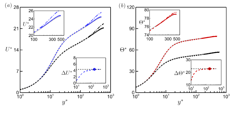
Figure 4: Comparison at $Re_{\tau_{0}}=590$ of (a) mean velocity $\overline{U}^{*}$, and (b) mean temperature $\overline{\Theta}^{*}$ between the full-domain channel flow (grey lines) and the reduced-domain channel flow (black, blue and red lines). Black lines: non-actuated case at $Pr=7.5$. Blue and red lines: travelling wave case at $Pr=7.5$ with $A^{+}=12$, $\kappa^{+}_{x}=0.0014$, $\omega^{+}=0.088$. For the reduced-domain cases, the resolved portion is shown with a dashed line ($y^{*}\lesssim 170$), and the unresolved portion is shown with a dashed-dotted line ($y^{*}\gtrsim 170$). The unresolved portion is replaced by the reconstructed profiles (solid lines), as explained in §2.3. The insets plot the velocity and temperature differences $\Delta\overline{U}^{*}$ and $\Delta\overline{\Theta}^{*}$; bullets mark $y^{*}_{\mathrm{res}}=170$, where we obtain the log-law shifts $\Delta\overline{U}^{*}_{\mathrm{log}}$ and $\Delta\overline{\Theta}^{*}_{\mathrm{log}}$.

2.3 Calculating the skin-friction coefficient and Stanton number

We can write the skin-friction coefficient and Stanton number as $C_{f}=2/{U^{*}_{b}}^{2}$ and $C_{h}=1/(U^{*}_{b}\Theta^{*}_{b})$. Although some studies use the mixed-mean temperature to define $C_{h}$ (MacDonald et al., 2019; Rouhi et al., 2022; Zhong et al., 2023), we use the bulk temperature $\Theta_{b}$ as adopted by Stalio & Nobile (2003) and Kuwata (2022), primarily because it is more straightforward to derive a predictive model for $HR$ with this definition (Appendix B). For our cases, there is only a maximum $2\%$ difference between $C_{h}$ based on $\Theta_{b}$ and the one based on the mixed-mean temperature.

For the full-domain channel flow, the mean velocity $\overline{U}^{*}$ and temperature $\overline{\Theta}^{*}$ are fully resolved across the entire channel (grey profiles in figure 4), and so $U^{*}_{b}$ and $\Theta^{*}_{b}$ can be obtained by direct integration of $\overline{U}^{*}$ and $\overline{\Theta}^{*}$. For the reduced-domain channel flow, we first need to construct $\overline{U}^{*}$ and $\overline{\Theta}^{*}$ beyond $y^{*}_{\mathrm{res}}$ (Rouhi et al., 2022, 2023). In figure 4, we see that the resolved portions of the $\overline{U}^{*}$ and $\overline{\Theta}^{*}$ profiles up to $y^{*}_{\mathrm{res}}\simeq 170$ are in excellent agreement with the full-domain profiles. Beyond $y^{*}_{\mathrm{res}}$, however, the flow is unresolved due to the domain truncation, appearing as a fictitious wake in the $\overline{U}^{*}$ and $\overline{\Theta}^{*}$ profiles (dashed-dotted lines in figure 4). We replace these unresolved portions with the composite profiles of $\overline{U}^{*}$ and $\overline{\Theta}^{*}$ (C1a, C1b in Appendix B). For this, we need the log-law shifts $\Delta\overline{U}^{*}_{\mathrm{log}}$ and $\Delta\overline{\Theta}^{*}_{\mathrm{log}}$ in (C1a) and (C1b), which we obtain by plotting $\Delta\overline{U}^{*}=\overline{U}^{*}-\overline{U}^{*}_{0}$ and $\Delta\overline{\Theta}^{*}=\overline{\Theta}^{*}-\overline{\Theta}^{*}_{0}$, the differences between the actuated and the non-actuated cases (see figure 4). Finally, we find $U^{*}_{b}$ and $\Theta^{*}_{b}$ by integrating the resolved portion of the profiles up to $y^{*}_{\mathrm{res}}$ and the reconstructed portion beyond $y^{*}_{\mathrm{res}}$. By applying this profile reconstruction, we obtain less than $1\%$ difference in $C_{f}$ and $C_{h}$ between the full-domain case and the reduced domain case (table 3 in Appendix A).

3 Results

3.1 Overall variations of $DR$ and $HR$

The values of $HR$, $DR$ and the difference $HR-DR$ are shown in figure 5. For all cases considered, $HR$ and $DR$ initially increase with the frequency of forcing, but for $\omega^{+}\gtrsim 0.04$ they reach a maximum value before slowly decreasing at higher frequencies. The maximum drag reduction is about $30\%$ for all Prandtl numbers, but the maximum heat-transfer reduction increases from 30% to about $40\%$ with increasing Prandtl number, marking a significant break from the Reynolds analogy. The comparison between the reduced-domain results (filled squares) and the full-domain results (open circles) supports the reliability of the production runs. At $Pr=7.5$, the reduced domain grid is more than twice as coarse as the full domain grid, yet there is less than $2\%$ difference in $DR$ and $HR$ (Appendix A gives more details). The trends in $DR$ seen here have been widely recorded in the previous literature, as the review by Ricco et al. (2021) makes clear. However, to the authors’ knowledge, the behaviour of $HR$ has not been reported before.

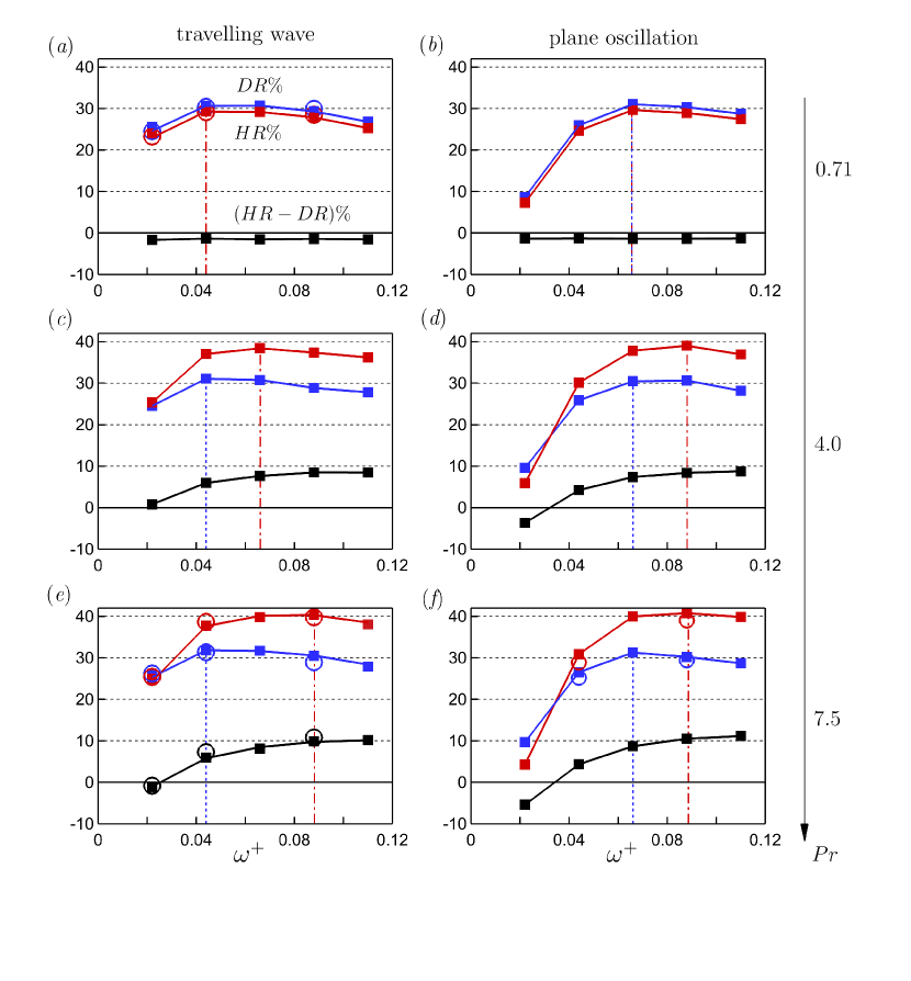
Figure 5: Values of $DR\%$ (blue symbols), $HR\%$ (red symbols) and their difference (black symbols) for the cases given in table 1. Filled squares: reduced domain simulations; empty circles: full domain simulations. Blue dashed line marks the maximum $DR$; red dashed-dotted line marks the maximum $HR$.

3.2 Optimal actuation frequency

Figure 5 indicates that the optimal actuation frequency for $DR$ is $\omega^{+}\approx 0.044$ for the travelling wave, and $\approx 0.066$ for the plane oscillation, regardless of the Prandtl number. For $HR$, the optimal frequency coincides with that for $DR$ at $Pr=0.71$, but it increases to $0.088$ for both types of actuation as the Prandtl number increase to 7.5.

Previous studies relate the optimal frequency for drag reduction to the characteristic time-scale of the energetic velocity scales associated with the near-wall cycle of turbulence, $\mathcal{T}^{+}_{u}$ (Jung et al., 1992; Quadrio et al., 2009; Quadrio & Ricco, 2011; Gatti & Quadrio, 2016; Chandran et al., 2023). When the actuation period $T^{+}_{osc}\equiv 2\pi/\omega^{+}$ matches this time scale, the wall oscillation becomes more effective in disrupting the near-wall scales, leading to the maximum $DR$ (Touber & Leschziner, 2012; Ricco et al., 2021). Chandran et al. (2023) discuss this interaction using the pre-multiplied spectrum of wall shear-stress $f^{+}\phi^{+}_{\tau\tau}$, and the corresponding spectra for our non-actuated channel flow case are shown in figure 6(a–c) (blue lines). In agreement with Chandran et al. (2023), the peaks in the shear-stress spectra occur at $\mathcal{T}^{+}_{u}\simeq 100$, corresponding to $\omega^{+}\simeq 0.063$, which broadly matches the frequencies of actuation for maximum drag reduction found here.

Figure 6 also shows the corresponding spectra for the fluctuating wall heat-flux, $f^{+}\phi^{+}_{qq}$ (red lines), as well as the pre-multiplied spectrograms of the fluctuating streamwise velocity and temperature ($k^{+}_{z}\phi^{+}_{uu},\ k^{+}_{x}\phi^{+}_{uu},\ k^{+}_{z}\phi^{+}_{\theta\theta},\ k^{+}_{x}\phi^{+}_{\theta\theta}$). Figures 6(a,b,c) reveal that while $f^{+}\phi^{+}_{qq}$ is sensitive to $Pr$ at small time-scales ($T^{+}\lesssim 70$), the time scale of the energetic temperature scales $\mathcal{T}^{+}_{\theta}\simeq 100$ is insensitive to $Pr$, and coincides with $\mathcal{T}^{+}_{u}$. The streamwise and spanwise lengths of the energetic temperature scales vary somewhat with Prandtl number (see figures 6d–i), but they also remain close to the length-scales of the energetic velocity scales. However, the peak in $k^{+}_{z}\phi^{+}_{\theta\theta}$ drops from $y^{+}=16$ at $Pr=0.71$ to $y^{+}=5$ at $Pr=7.5$, as the conductive sublayer thins with increasing Prandtl number (Alcántara-Ávila & Hoyas, 2021; Kader, 1981; Schwertfirm & Manhart, 2007).

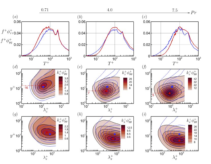
Figure 6: Non-actuated channel flow with increasing Prandtl number. (a,d,g) $Pr=0.71$; (b,e,h) $Pr=4.0$; (c,f,i) $Pr=7.5$. (a–c) Pre-multiplied frequency spectra of wall shear-stress $f^{+}\phi^{+}_{\tau\tau}$ (blue line) and wall heat-flux $f^{+}\phi^{+}_{qq}$ (red line), where $T^{+}=1/f^{+}$. (d–f) Spectrograms of the streamwise velocity fluctuations (blue contour lines) and temperature fluctuations (filled contour) pre-multiplied by the spanwise wavenumber $k^{+}_{z}$. (g–i) Same as (d–f), pre-multiplied by the streamwise wavenumber $k^{+}_{x}$. Contour levels for $k^{+}_{z}\phi^{+}_{uu}$ start from $0.2$ to $3.8$ with an increment of $0.6$; contour levels for $k^{+}_{x}\phi^{+}_{uu}$ start from $0.2$ to $2.2$ with an increment of $0.4$. The blue and red bullets in (d–f) locate the maximum in $k^{+}_{z}\phi^{+}_{uu}$ and $k^{+}_{z}\phi^{+}_{\theta\theta}$, respectively, and in (g–i) locate the maximum in $k^{+}_{x}\phi^{+}_{uu}$ and $k^{+}_{x}\phi^{+}_{\theta\theta}$, respectively.

For the plane oscillation, we expect that the maximum $DR$ and $HR$ is achieved when the actuation period is close to $\mathcal{T}^{+}_{u}$ and $\mathcal{T}^{+}_{\theta}$, respectively. For the travelling wave, however, the optimal actuation period cannot be directly compared with $\mathcal{T}^{+}_{u}$ or $\mathcal{T}^{+}_{\theta}$, owing to the relative streamwise motion between the travelling wave and the advecting near-wall scales. As discussed by Karniadakis & Choi (2003), Quadrio et al. (2009) and Quadrio & Ricco (2011), for maximum $DR$, $\mathcal{T}^{+}_{u}$ must be compared with a relative oscillation period $2\pi/(\kappa^{+}_{x}\mathcal{U}^{+}_{u}+\omega^{+})$ as seen by an observer travelling with the convection speed of the near-wall energetic velocity scales $\mathcal{U}^{+}_{u}$. Similarly, for maximum $HR$, $\mathcal{T}^{+}_{\theta}$ must be compared with $2\pi/(\kappa^{+}_{x}\mathcal{U}^{+}_{\theta}+\omega^{+})$, where $\mathcal{U}^{+}_{\theta}$ is the convection speed of the near-wall energetic temperature scales. After some recasting (using $\mathcal{T}^{+}_{u}\simeq\mathcal{T}^{+}_{\theta}\simeq 100$, $\kappa^{+}_{x}=0.0014$), we estimate the optimum frequencies of actuation for $DR$ and $HR$ to be, respectively,

$$\omega^{+}_{\mathrm{opt},DR} =\frac{2\pi}{\mathcal{T}^{+}_{u}}-\kappa^{+}_{x}\mathcal{U}^{+}_{u}\simeq 0.046,$$ (3.1a)

$$\omega^{+}_{\mathrm{opt},HR} =\frac{2\pi}{\mathcal{T}^{+}_{\theta}}-\kappa^{+}_{x}\mathcal{U}^{+}_{\theta}\simeq 0.063-0.0014\mathcal{U}^{+}_{\theta},$$ (3.1b)

where we have assumed that $\mathcal{U}^{+}_{u}$ follows a universal curve (Kim & Hussain, 1993; Del Álamo & Jiménez, 2009; Liu & Gayme, 2020), where $\mathcal{U}^{+}_{u}\simeq 12$ at $y^{+}\simeq 15$ (marked with blue bullets in figures 6d–i).

The estimated optimum frequency for $DR$ is independent of Prandtl number, at about $0.046$, consistent with our DNS results for the travelling wave case (figures 5a,c,e). However, the optimum frequency for $HR$ depends on $Pr$, since we expect that $\mathcal{U}^{+}_{\theta}$ decreases as the energetic temperature scales move closer to the wall with increasing Prandtl number (red bullets in figure 6d–i). Hetsroni et al. (2004) computed the profiles of $\mathcal{U}^{+}_{\theta}$ at $Pr=1.0$, 5.4 and 54 in a configuration similar to that used in the present study, without actuation. Using their results, we estimate that $\mathcal{U}^{+}_{\theta}$ decreases from $12$ to $6$ as $Pr$ increases from $0.71$ to $7.5$, which gives $\omega^{+}_{\mathrm{opt},HR}=0.046$ at $Pr=0.71$ and $0.055$ at $Pr=7.5$. The estimated value at $Pr=7.5$ is smaller than the value of 0.088 given by the DNS (figure 5e), but the trends with Prandtl number are consistent. In §3.6 and 3.7, we conduct a more quantitative justification for the trends in $\omega^{+}_{\mathrm{opt},HR}$ by considering the interaction between the Stokes layer and the near-wall thermal field.

3.3 Mean profiles and turbulence statistics

We now consider the distributions of the mean velocity $\overline{U}^{*}$ ($=\overline{U}/u_{\tau}$), the mean temperature $\overline{\Theta}^{*}$ ($=\overline{\Theta}/\theta_{\tau}$) (figure 7), and the velocity and temperature statistics (figure 8) as we vary $\omega^{+}$ and $Pr$. We focus on the travelling wave case, but since the observed trends are consistent with those from the plane oscillation case (figures 25 and 26 in Appendix C), our conclusions are applicable to both types of actuation.

Figure 7: Travelling wave actuation with $A^{+}=12$, $\kappa^{+}_{x}=0.0014$. Left column: $DR\%$ and $\overline{U}^{*}$ profiles, where $\Delta\overline{U}^{*}=\overline{U}^{*}-\overline{U}^{*}_{0}$ (results independent of $Pr$). Middle and right columns correspond to $Pr=0.71$ and $7.5$, respectively: $DR\%$ (blue line), $HR\%$ (red line), and $\overline{\Theta}^{*}$ profiles, where $\Delta\overline{\Theta}^{*}=\Theta^{*}-\Theta^{*}_{0}$. In the panels (d–l), the thin black line is the reference (non-actuated) case, the blue lines and the red lines show the effects of increasing $\omega^{+}$ on $\overline{U}^{*}$ and $\overline{\Theta^{*}}$, respectively, and the thick dashed line corresponds to $DR_{\mathrm{max}}$ or $HR_{\mathrm{max}}$. In (j,k,l), the black cross symbols mark the distance $y^{*}$ where $\Delta\overline{U}^{*}$ or $\Delta\Theta^{*}$ reach $0.95$ of their values at $y^{*}=170$.

It is well known from the literature that drag reduction by spanwise wall oscillation coincides with the thickening of the viscous sublayer (Touber & Leschziner, 2012; Hurst et al., 2014; Gatti & Quadrio, 2016; Chandran et al., 2023; Rouhi et al., 2023). This is evident also from our $\overline{U}^{*}/y^{*}$ profiles (figure 7g), where the actuated profiles (blue profiles) depart from unity farther from the wall compared to the non-actuated profile (black profile). The conductive sublayer also thickens with wall oscillation, but it then thins substantially with increasing Prandtl number, so that at $Pr=7.5$ the conductive sublayer is substantially thinner than the viscous sublayer (figure 7i).

Viscous sublayer and conductive sublayer thickening due to the wall oscillation shifts the $\overline{U}^{*}$ and $\overline{\Theta}^{*}$ profiles. This is shown in figure 7(j,k,l) where we plot the differences $\Delta\overline{U}^{*}=\overline{U}^{*}-\overline{U}^{*}_{0}$ and $\Delta\overline{\Theta}^{*}=\overline{\Theta}^{*}-\overline{\Theta}^{*}_{0}$ between the actuated and the non-actuated cases. The cases with the maximum $DR$ (or $HR$) have the highest $\Delta\overline{U}^{*}$ (or $\Delta\overline{\Theta}^{*}$), as highlighted by the thick dashed line in the plots. According to Rouhi et al. (2023), the distance $y^{*}$ where $\Delta\overline{U}^{*}$ reaches a plateau indicates the extent to which the Stokes layer disturbs the $\overline{U}^{*}$ profile. In figure 7(j,k,l), therefore, we mark each profile at the $y^{*}$ location where $\Delta\overline{U}^{*}$ (or $\Delta\overline{\Theta}^{*}$) reaches $95\%$ of its value at $y^{*}=170$. We find that the distance to reach the plateau in $\Delta\overline{\Theta}^{*}$ depends on $\omega^{+}$ and $Pr$ (compare figures 7k,l), where the plateau is reached at a lower $y^{*}$ with increasing Prandtl number.

Figure 8: Travelling wave actuation with $A^{+}=12$, $\kappa^{+}_{x}=0.0014$. Notation and symbols as in figure 7. Here, $\Delta\overline{uv}^{*}=\overline{uv}^{*}-\overline{uv}^{*}_{0}$, and $\Delta\overline{\theta v}^{*}=\overline{\theta v}^{*}-\overline{\theta v}^{*}_{0}$. In (d,e,f), the numbers give the $y^{*}$ location of the inner-peak in the $\overline{u^{2}}^{*}$ and $\overline{\theta^{2}}^{*}$ profiles. In (g–l), the vertical dashed line locates the peak of non-actuated $\overline{uv}^{*}_{0}$ (g,j) and $\overline{\theta v}^{*}_{0}$ (h,i,k,l).

In figure 8, we plot the turbulence statistics for the same cases shown in figure 7. Drag reduction and viscous sublayer thickening (figures 7a,d,g) coincide with the near-wall attenuation of $\overline{u^{2}}^{*}$ and the shift in its inner peak (figure 8d), as known from previous work (Touber & Leschziner, 2012; Ricco et al., 2021; Rouhi et al., 2023). Similarly, we find that at each $Pr$, heat-transfer reduction and conductive sublayer thickening (figures 7b,c,e,f,h,i) coincide with the near-wall attenuation of $\overline{\theta^{2}}^{*}$ and the shift in its inner peak (figures 8e,f). Interestingly, $DR_{\mathrm{max}}$ occurs when the inner peak in $\overline{u^{2}}^{*}$ is located farthest from the wall, and a similar connection exists between $HR_{\mathrm{max}}$ and the location of the inner peak in $\overline{\theta^{2}}^{*}$ (compare the listed numbers in figures 8d,e,f).

Figure 9: Travelling wave actuation with $A^{+}=12$, $\kappa^{+}_{x}=0.0014$, $\omega^{+}=0.088$ at $Pr=7.5$. (a) Terms in the averaged streamwise momentum equation (3.3a). (b) Terms in the averaged temperature equation (3.3b).

In addition, the attenuation of the turbulent shear-stress $\overline{uv}^{*}$ (figure 8g) and the wall-normal turbulent temperature-flux $\overline{\theta v}^{*}$ (figures 8h,i) are directly linked to $DR$ and $HR$, respectively. In figure 8(j,k,l), we plot the differences between the actuated and non-actuated cases $\Delta\overline{uv}^{*}=\overline{uv}^{*}-\overline{uv}^{*}_{0}$ and $\Delta\overline{\theta v}^{*}=\overline{\theta v}^{*}-\overline{\theta v}^{*}_{0}$. Most of the attenuation occurs near the wall, with the maxima occurring near $y^{*}\simeq 10$. For $y^{*}>10$, the attenuation declines, and $\Delta\overline{uv}^{*}$ and $\Delta\overline{\theta v}^{*}$ reach local minima at points that coincide approximately with the locations of the peaks in $\overline{uv}^{*}_{0}$ and $\overline{\theta v}^{*}_{0}$.

By integrating the plane- and time-averaged streamwise momentum (6) and temperature (7) equations from zero to $y^{*}$, we obtain

$$\frac{d\overline{U}^{*}}{dy^{*}}=\overline{uv}^{*}+\left(1-y^{*}Re_{\tau}^{-1}\right),\qquad\frac{d\overline{\Theta}^{*}}{dy^{*}}=Pr\,\left[\overline{\theta v}^{*}+\left(1-y^{*}Re_{\tau}^{-1}\right)+\mbox{Res}_{\Theta}\right],$$ (3.2a,b)

where $\mbox{Res}_{\Theta}\equiv Re^{-1}_{\tau}\int_{0}^{y^{*}}(1-\overline{U}^{*}/U^{*}_{b})dy^{\prime}$. Hence,

$$\frac{d(\Delta\overline{U}^{*})}{dy^{*}} =\Delta\overline{uv}^{*}-y^{*}\left({Re_{\tau}^{-1}}-{Re_{\tau_{0}}^{-1}}\right),$$ (3.3a)

$$\frac{d(\Delta\overline{\Theta}^{*})}{dy^{*}} =Pr\,\left[\Delta\overline{\theta v}^{*}-y^{*}\left({Re_{\tau}^{-1}}-{Re_{\tau_{0}}^{-1}}\right)+\underbrace{\Delta\mbox{Res}_{\Theta}}_{\simeq 0}\right].$$ (3.3b)

The difference $\Delta\mbox{Res}_{\Theta}$ between the actuated and the non-actuated cases is small and can be neglected. The remaining terms in (3.3a) and (3.3b) are plotted in figure 9 for the travelling wave case at $Pr=7.5$ and $\omega^{+}=0.088$. We see that the right-hand-side of (3.3a) and (3.3b) are dominated by $\Delta\overline{uv}^{*}$ and $\Delta\overline{\theta v}^{*}$, up to their respective minima, but farther from the wall these terms are cancelled by the term containing the difference in Reynolds numbers $\left({Re_{\tau}^{-1}}-{Re_{\tau_{0}}^{-1}}\right)$. That is, the net contributions to $\Delta\overline{U}^{*}$ and $\Delta\overline{\Theta}^{*}$, hence $DR$ and $HR$, come from $\Delta\overline{uv}^{*}$ and $\Delta\overline{\theta v}^{*}$, and then only up to the points where $\Delta\overline{uv}^{*}$ and $\Delta\overline{\theta v}^{*}$ reach their minimum values.

3.4 Source of inequality between $HR$ and $DR$

Integrating (3.3a) and (3.3b) once more with respect to $y^{*}$ gives

$$\Delta\overline{U}^{*}_{y^{*}}=\int_{0}^{y^{*}}\Delta^{*}_{uv}dy^{\prime},\qquad\Delta\overline{\Theta}^{*}_{y^{*}}=Pr\int_{0}^{y^{*}}\Delta^{*}_{\theta v}dy^{\prime},$$ (3.4a,b)

where

$$\Delta^{*}_{uv} \equiv\Delta\overline{uv}^{*}-y^{*}(Re_{\tau}^{-1}-Re_{\tau_{0}}^{-1}),$$ (3.4c)

$$\Delta^{*}_{\theta v} \equiv\Delta\overline{\theta v}^{*}-y^{*}(Re_{\tau}^{-1}-Re_{\tau_{0}}^{-1}).$$ (3.4d)

By using (3.4a,b) we can relate $\Delta^{*}_{uv}$ and $\Delta^{*}_{\theta v}$ to $\Delta\overline{U}^{*}$ and $\Delta\overline{\Theta}^{*}$, hence to $DR$ and $HR$, and so establish the connection between the drag and heat-transfer reduction and the turbulence attenuation. For the drag reduction, Gatti & Quadrio (2016) derived the relation between $DR$ ($=1-R_{f}$) and the asymptotic value of $\Delta\overline{U}^{*}$ in the log region (3.5a). In Appendix B, we derive a similar relation between $HR$ ($=1-R_{h}$) and the asymptotic value of $\Delta\overline{\Theta}^{*}$ in the log region (3.5b). That is, we have

$$\Delta\overline{U}^{*}_{170} =\sqrt{\frac{2}{C_{{f_{0}}}}}\left[\frac{1}{\sqrt{R_{f}}}-1\right]-\frac{1}{2\kappa_{u}}\ln{R_{f}}=\underbrace{\int^{170}_{0}\Delta^{*}_{uv}dy^{\prime}}_{I_{uv}}$$ (3.5a)

$$\Delta\overline{\Theta}^{*}_{170} =\frac{\sqrt{C_{{f_{0}}}/2}}{C_{{h_{0}}}}\left[\frac{\sqrt{R_{f}}}{R_{h}}-1\right]-\frac{1}{2\kappa_{\theta}}\ln{R_{f}}=Pr\underbrace{\int^{170}_{0}\Delta^{*}_{\theta v}dy^{\prime}}_{I_{\theta v}}$$ (3.5b)

These derivations assume that the profiles of $\overline{U}^{*}$ and $\overline{\Theta}^{*}$ have well-defined log regions with slopes that are not affected by the wall oscillation, which is the case for our results (figure 7). The integration was performed up to $y^{*}_{\mathrm{res}}=170$, where the profiles of $\Delta\overline{U}^{*}$ and $\Delta\overline{\Theta}^{*}$ reach their asymptotic levels (figures 7j,k,l) and their derivatives are zero (figure 9). On the right-hand-sides of (3.5a) and (3.5b) we have the integrals of attenuation in the turbulent shear-stress ($I_{uv}$) and the turbulent temperature-flux ($I_{\theta v}$). For a fixed set of viscous-scaled actuation parameters, $I_{uv}$ is constant (Touber & Leschziner, 2012; Hurst et al., 2014; Gatti & Quadrio, 2016; Rouhi et al., 2023), but $I_{\theta v}$ depends on $Pr$ in addition to the actuation parameters (figures 8k,l).

To predict $DR$ and $HR$ from (3.5a) and (3.5b), we only need $\Delta\overline{U}^{*}_{170}$ and $\Delta\overline{\Theta}^{*}_{170}$ (that is, $I_{uv}$ and $I_{\theta v}$) as the inputs; the other parameters are associated with the non-actuated channel flow for which semi-empirical relations exist in the literature. We choose $\kappa_{u}=0.4$ and $\kappa_{\theta}=0.46$ (Pirozzoli et al., 2016); the suitability of these choices is confirmed in §2.3 and Appendix A. Dean (1978)’s correlation is used for the non-actuated skin-friction coefficient $C_{{f_{0}}}=0.037Re^{-0.29}_{\tau_{0}}$; this correlation agrees well with the DNS data (MacDonald et al., 2019). For the non-actuated $C_{{h_{0}}}$, we adopt the predictive formula given by Pirozzoli et al. (2022) and Pirozzoli (2023), where

$$\frac{1}{C_{{h_{0}}}}=\frac{\kappa_{u}}{\kappa_{\theta}}\frac{2}{C_{{f_{0}}}}+\left(\beta_{CL}-\beta_{2}-\frac{\kappa_{u}}{\kappa_{\theta}}B\right)\sqrt{\frac{2}{C_{{f_{0}}}}}+\beta_{3}.$$ (3.6)

Here $\beta_{CL}(Pr)=B_{\theta}(Pr)+3.504-1.5/\kappa_{\theta}$, $\beta_{2}=4.92$, $\beta_{3}=39.6$, $B=1.23$, and $B_{\theta}(Pr)$ is the log-law additive constant for $\overline{\Theta}^{*}$ (Kader & Yaglom, 1972), as introduced in Appendix B. Pirozzoli (2023) showed that (3.6) agrees well with DNS data for $\mathcal{O}(10^{-2})\lesssim Pr\lesssim\mathcal{O}(10^{1})$.

Figure 10: Travelling wave actuation with $A^{+}=12$, $\kappa^{+}_{x}=0.0014$. Comparison between the direct $HR$ from DNS (filled squares) and the predicted $HR$ (empty triangles) by solving (3.5a) and (3.5b). In (a) for predicting $HR$ we use $I_{uv}$ and $I_{\theta v}$ directly from DNS. In (b) for predicting $HR$ we use a power-law estimate for $I_{\theta v}=I_{uv}/Pr^{\gamma}$, with the values of $\gamma$ reported in figure 11(b).

Figure 11: Travelling wave at $Pr=0.71,4.0$ and $7.5$ (same data as in figure 5a,c,e). The outline colour of each data point indicates its $\omega^{+}$; $\omega^{+}=0.022$ (black), $0.044$ (blue), $0.066$ (red), $0.088$ (green) and $0.110$ (grey). (a) $I_{\theta v}$ versus $I_{uv}$; the dotted line is for $I_{\theta v}=I_{uv}$. (b) $I_{\theta v}$ versus $Pr$; the solid curves are the power-law fit $I_{\theta v}=I_{uv}/Pr^{\gamma}$, with $\gamma$ as shown. (c,d) $HR$ and $HR-DR$ versus $Pr$; the solid curves are the prediction of (3.5b) using $I_{\theta v}=I_{uv}/Pr^{\gamma}$. In (d) blue zone marks $\gamma>0.5$, grey zone marks $\gamma<0.5$.

In figure 10(a), we compare the values of $HR$ from DNS with those from (3.5a) and (3.5b) using $I_{uv}$ and $I_{\theta v}$ as obtained from DNS. The results support the accuracy of the model for relating $HR$ to the attenuation of the turbulent flux. In figure 10(b), we also show the agreement between the model and the DNS when we use a power law estimate for $I_{\theta v}$ ($=I_{uv}/Pr^{\gamma}$) where only $I_{uv}$ (which is independent of $Pr$) is obtained from DNS. We justify the power law as follows.

From (3.5b), we note that the Prandtl number dependence of $HR$ (hence $HR-DR$) is due to both $C_{{h_{0}}}$ and $I_{\theta v}$. According to the Reynolds analogy, we would expect $I_{\theta v}=I_{uv}$ when $Pr=1.0$. Figure 11(a) indicates that, regardless of the actuation frequency $\omega^{+}$, $I_{\theta v}>I_{uv}$ for $Pr=0.71$, and $I_{\theta v}<I_{uv}$ for $Pr>1$, with the difference increasing with $Pr$. In other words, increasing $Pr$ beyond unity leads to a lower attenuation of $\overline{\theta v}$ compared to $\overline{uv}$, even though in this regime $HR>DR$ (figure 5c–f). Figure 11(b) shows how $I_{\theta v}$ depends on $Pr$, and that $I_{\theta v}=I_{uv}/Pr^{\gamma}$ is a good approximation to the data, where $\gamma$ depends on $\omega^{+}$ but is independent of $Pr$. When we use this power law in (3.5b) and solve for $HR$ by using $I_{uv}$ from DNS, figures 11(c,d) show that the model closely matches the data. Furthermore, for $\gamma<0.5$ we can achieve $HR>DR$ for $Pr>1$, and the smaller $\gamma$ is the higher $HR$ is compared to $DR$. From figures 11(b,d), as $\omega^{+}$ increases from $0.022$ (black curve) to $0.110$ (grey curve), $\gamma$ decreases from about $0.5$ to $0.1$, and $HR-DR$ increases from almost zero to $10\%$. Therefore, we expect $HR<DR$ for $Pr>1.0$ if $\gamma>0.5$. This occurs for the plane oscillation at $\omega^{+}=0.022$, where $\gamma=2.43$ and $HR-DR\simeq-5\%$ (figure 19).

Figure 12: Predicted maps of (a) $HR$ and (b) $HR-DR$ for the travelling wave with $A^{+}=12,\kappa^{+}_{x}=0.0014$ and $\omega^{+}=0.088$. The white bullets represent DNS results at $Re_{\tau_{0}}=590$ for $Pr=0.71,4.0,7.5$ and $20$.

3.5 Heat transfer reduction at higher Prandtl number and Reynolds number

Gatti & Quadrio (2016) used (3.5a) to extrapolate their low Reynolds number $DR$ data to higher Reynolds numbers, and the accuracy of this extrapolation up to $Re_{\tau_{0}}=4000$ was corroborated by Rouhi et al. (2023) using large-eddy simulation. For a fixed set of actuation parameters $(A^{+},\kappa^{+}_{x},\omega^{+})$, $I_{uv}$ is Reynolds and Prandtl number independent, and so the only Reynolds number dependency of $DR$ is through $C_{f_{0}}$. Hence, Gatti & Quadrio (2016) could solve (3.5a) and predict $DR$ at any Reynolds number. We can now do the same for $HR$ by using the power law relationship $I_{\theta v}=I_{uv}/Pr^{\gamma}$. By knowing $I_{uv}$ and $\gamma$ for a fixed set of actuation parameters, we can then solve (3.5a) and (3.5b) to map $HR$ and $HR-DR$ as functions of $Pr$ and $Re_{\tau_{0}}$.

In figure 12, we show these predictions for the travelling wave case with $\omega^{+}=0.088$, where the DNS gives $I_{uv}=4.28$ and $\gamma=0.16$ (data points with green outline in figure 11). The predictions agree well with the DNS data points, including the point at $Pr=20$ ($HR=43\%,HR-DR=13\%$) (see table 4). At a given Reynolds number, $HR$ increases almost logarithmically with Prandtl number. For instance, at $Re_{\tau_{0}}=590$ $HR$ increases from $30\%$ to $40\%$ as the Prandtl number increases from 0.71 to 7.5, and $HR=50\%$ would be obtained at a Prandtl number of about 75. In addition, $HR$ decreases very slowly with increasing $Re_{\tau_{0}}$. For instance, at $Pr=7.5$ $HR$ decreases from $40\%$ to about $36\%$ as $Re_{\tau_{0}}$ increases from $590$ to $5900$. Such a slow decrease with $Re_{\tau_{0}}$ is similarly observed in the predictive model for $DR$ (3.5a) (Marusic et al., 2021; Chandran et al., 2023; Rouhi et al., 2023).

We now examine the near-wall turbulence to help understand why $I_{\theta v}<I_{uv}$ for $Pr>1$.

3.6 Stokes layer interaction with the velocity and thermal fields: integral parameters

In the inner-scaled actuation pathway $(\omega^{+}\gtrsim 0.018)$, the protrusion of the Stokes layer due to the wall oscillation modifies the near-wall velocity field and leads to $DR$ (Quadrio & Ricco, 2011; Ricco et al., 2021; Rouhi et al., 2023), and we would expect that a similar interaction between the Stokes layer and the near-wall temperature field leads to $HR$. In this respect, Rouhi et al. (2023) found that the Stokes layer protrusion modifies the near-wall $\overline{u^{2}}^{*}$ profiles (figure 8d), and similar trends are seen in the $\overline{\theta^{2}}^{*}$ profiles (figures 8e,f). To determine how the Stokes layer affects $I_{uv}$ and $I_{\theta v}$ as the Prandtl number changes, we first identify the Stokes layer characteristics through the harmonic component of the spanwise velocity $\overline{\tilde{w}^{2}}$, where $\tilde{w}$ is obtained by applying triple decomposition

$$W(x,y,z,t)=\overline{W}(y)+\tilde{w}(x,y,t)+w(x,y,z,t),$$ (3.7a)

$$\tilde{w}(x,y,t)=\underbrace{\frac{1}{N}\sum_{n=0}^{N-1}W(x,y,t+nT_{osc})}_{\left<W\right>(x,y,t)}-\overline{W}(y).$$ (3.7b)

Here, $\overline{W}$ is the plane- and time-averaged component of the spanwise velocity, $\tilde{w}$ is the harmonic component, $w$ is the turbulent component, and $\left<W\right>$ is the spanwise and phase averaged value of $W$. For the streamwise and wall-normal velocities and the temperature field, the harmonic components are negligible compared the turbulent components. Following Rouhi et al. (2023), we quantify the Stokes layer protrusion height $\ell^{*}_{0.01}$ as the wall distance where $\overline{\tilde{w}^{2}}^{*}=0.01$, and we locate the Stokes layer thickness $\delta^{*}_{S}$ where $\overline{\tilde{w}^{2}}^{*}=\frac{1}{2}{A^{*}}^{2}\mathrm{e}^{-2}$. We also calculate the production due to the Stokes layer according to $P^{*}_{33}\equiv-2\overline{\left<wv\right>\partial\tilde{w}/\partial y}^{*}-2\overline{\left<wu\right>\partial\tilde{w}/\partial x}^{*}$, where $P^{*}_{33}$ is the only external source term due to the Stokes layer that injects energy into the turbulent stress budgets (Touber & Leschziner, 2012; Umair et al., 2022).

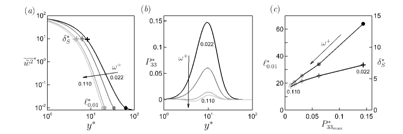
Figure 13: Characteristics of the Stokes layer for the travelling wave with $A^{+}=12,\kappa^{+}_{x}=0.0014$ and $0.022\leq\omega^{+}\leq 0.110$ (same cases as in figure 5a,c,e). Results are independent of Prandtl number. The colour of the profiles and data points change from black at $\omega^{+}=0.022$ to light grey at $\omega^{+}=0.110$. (a) Profiles of $\overline{\tilde{w}^{2}}^{*}$. Stokes layer protrusion height $\ell^{*}_{0.01}$ (Rouhi et al., 2023) marked at $\overline{\tilde{w}^{2}}^{*}=0.01$ (filled bullets); laminar Stokes layer thickness $\delta^{*}_{S}$ marked at $\overline{\tilde{w}^{2}}^{*}=\frac{1}{2}{A^{*}}^{2}\mathrm{e}^{-2}$ (cross symbols). (b) Production due to the Stokes layer $P^{*}_{33}$. (c) $\ell^{*}_{0.01}$ (filled bullets) and $\delta^{*}_{S}$ (cross symbols) versus the maximum value of $\tilde{P}^{*}_{33}$.

The behaviour of these Stokes layer parameters is given in figure 13, for the same travelling wave cases shown in figure 5(a,c,e). The profiles do not depend on $Pr$, that is, at a fixed $\omega^{+}$ the Stokes layer structure remains unchanged as the Prandtl number changes. When $\omega^{+}$ decreases, $\ell^{*}_{0.01}$ and the maximum production increase proportionately (figure 13c). In other words, the Stokes layer becomes more protrusive while injecting more energy into the turbulent field. We note that $\ell^{*}_{0.01}$ is almost linearly proportional to $P^{*}_{{33}_{\mathrm{max}}}$, but $\delta^{*}_{S}$ is less responsive to the rise in the production. Therefore, $\ell^{*}_{0.01}$ better quantifies the Stokes layer protrusion and strength, as sensed by the turbulent field, in agreement with the observations by Rouhi et al. (2023).

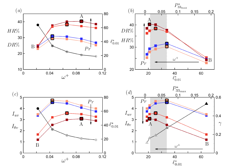
Figure 14: Variation of the integral parameters with the Stokes layer characteristics $(\ell^{*}_{0.01},P^{*}_{{33}_{\mathrm{max}}})$ for the same travelling wave cases as in figure 13. (a) $DR$ (blue squares), $HR$ (light orange to brick red squares), $\ell^{*}_{0.01}$ (black to grey bullets) versus $\omega^{+}$. (b) Same data as in (a) versus $\ell^{*}_{0.01}$ (bottom axis) and $P^{*}_{{33}_{\mathrm{max}}}$ (top axis). (c,d) correspond to (a,b) for $I_{uv}$ (blue squares) and $I_{\theta v}$ (light orange to brick red squares); in (d) we overlay $\gamma$ (grey to black triangles). In all plots, the colour of $HR$ and $I_{\theta v}$ changes from light orange at $Pr=0.71$ to brick red at $Pr=7.5$. The points associated with $DR_{\mathrm{max}}$ and $HR_{\mathrm{max}}$ are highlighted with a larger symbol size and black outline. In (b,d), the grey region shades the range of $DR_{\mathrm{max}}$ and $HR_{\mathrm{max}}$. In all plots we highlight two cases that we further analyse in figures 15 and 16: Case A at $\omega^{+}=0.088$ with $\gamma=0.16$, and Case B at $\omega^{+}=0.022$ with $\gamma=0.53$.

In figure 14, we assess the relation between the integral quantities $DR$, $HR$, $I_{\theta v}$, $I_{uv}$, and the Stokes layer characteristics. Rouhi et al. (2023) showed that $DR$ increases with $\ell^{*}_{0.01}$ up to an optimal value for maximum $DR$, corresponding to an optimal level of $P^{*}_{{33}_{\mathrm{max}}}$. For our present cases, this optimal point is $\ell^{*}_{0.01}=34$ (figure 14b), where protrusion beyond this point causes $DR$ to decrease. We observe a similar trend in $HR$ (figure 14b), but the corresponding optimal value of $\ell^{*}_{0.01}$ for maximum $HR$ decreases from 34 to 21 as the Prandtl number increases from 0.71 to 7.5. Figures 14(c,d) show that the variations of $I_{uv}$ and $I_{\theta v}$ with $\omega^{+}$ and $\ell^{*}_{0.01}$ are consistent with the trends in $DR$ and $HR$. In terms of variations with $Pr$, however, $HR$ increases even as $I_{\theta v}$ decreases. From $Pr=0.71$ to $7.5$, the maximum value of $I_{\theta v}$ shifts to smaller values of $\ell^{*}_{0.01}$, corresponding to a shift in $\omega^{+}$ from 0.044 ($\ell^{*}_{0.01}=34$) to 0.088 ($\ell^{*}_{0.01}=21$). Finally, it appears that the exponent $\gamma$ in the power law increases almost linearly with $\ell^{*}_{0.01}$ and $P^{*}_{33_{\mathrm{max}}}$ (figure 14d).

To summarise, we find that for $Pr>1$, achieving maximum $HR$ requires a less protrusive Stokes layer than achieving maximum $DR$. As the Stokes layer becomes more protrusive (energetic), it loses its efficacy in attenuating $\overline{\theta v}^{*}$ relative to $\overline{uv}^{*}$, that is, $\gamma$ increases as $\ell^{*}_{0.01}$ increases.

3.7 Stokes layer interaction with the velocity and thermal fields: scale-wise analysis

To better understand our observations on the integral parameters shown in figure 14, we now examine the spectrograms of $\overline{uv}^{*}$ and $\overline{\theta v}^{*}$ and visualise the distributions of the instantaneous $uv$ and $\theta v$ near the wall. We focus on two cases at $Pr=7.5$, Case A at $\omega^{+}=0.088$, where $HR$ is maximum and $DR$ is near maximum ($\gamma=0.16$), and Case B at $\omega^{+}=0.022$, where $HR$ and $DR$ drop below their maximum values, owing to a highly protrusive Stokes layer ($\gamma=0.53$).

Figure 15: Comparisons between Case A (left two columns) and Case B (right two columns. (a,m) Profiles of $\Delta^{*}_{uv}$ (blue) and $\Delta^{*}_{\theta v}$ (red). (b,n) Profiles of $\overline{\tilde{w}^{2}}^{*}$ (dashed-dotted line) and $P^{*}_{33}$ (solid line). Streamwise spectrograms: (c,o) $-k^{*}_{x}\phi^{*}_{uv}$; (d,p) $-k^{*}_{x}\phi^{*}_{\theta v}$ (contour lines and contour fields represent non-actuated and actuated cases, respectively). Difference between the actuated and the non-actuated cases for the wavenumber spectra (e,f,q,r), and frequency spectra (g,h,s,t). Spanwise spectrograms: (i,u) $-k^{*}_{z}\phi^{*}_{uv}$; (j,v) $-k^{*}_{z}\phi^{*}_{\theta v}$. Difference between the actuated and the non-actuated cases (k,l,w,x). In all the spectrgrams, the horizontal dashed line marks $\ell^{*}_{0.01}$.

Figure 15 displays the various pre-multiplied spectrograms for these two cases, where $\phi$ is the spectral density, $k_{x}$ is the streamwise wavenumber, $k_{z}$ is the spanwise wavenumber, and $f$ is the frequency. The differences between the actuated and the non-actuated cases are denoted by, for example, $\Delta k^{*}_{x}\phi^{*}_{uv}=k^{*}_{x}\phi^{*}_{uv}-k^{*}_{x}\phi^{*}_{{uv}_{0}}$. The extent up to which $\Delta k^{*}_{x}\phi^{*}_{uv}$ and $\Delta k^{*}_{x}\phi^{*}_{\theta v}$ are non-zero (red and blue fields in figures 15e,f,q,r) coincides with the height of the Stokes layer protrusion $\ell^{*}_{0.01}$ (horizontal dashed line); this supports the robustness of $\ell^{*}_{0.01}$ to measure the extent up to which the Stokes layer modifies the turbulent field. Overall, for both Cases A and B, and $k^{*}_{x}\phi^{*}_{uv}$ and $k^{*}_{x}\phi^{*}_{\theta v}$, the Stokes layer protrusion (production) leads to two outcomes: (1) large-scale energy attenuation as a favourable outcome (positive $\Delta k^{*}_{x}\phi^{*}_{uv},\Delta k^{*}_{x}\phi^{*}_{\theta v}$ for $\lambda^{*}_{x}\gtrsim 350$, shown as the red fields in figures 15e,f,q,r), and (2) small-scale energy amplification as an unfavourable outcome (negative $\Delta k^{*}_{x}\phi^{*}_{uv},\Delta k^{*}_{x}\phi^{*}_{\theta v}$ for $\lambda^{*}_{x}\lesssim 350$, shown as the blue fields). The large-scale energy attenuation corresponds to the attenuation of the near-wall streaks with $\lambda^{*}_{x}\simeq 10^{3}$ (see the energetic peaks in the non-actuated spectrograms). The small-scale energy amplification corresponds to the emergence of smaller scales with $\lambda^{*}_{x}\simeq 10^{2}$ (figures 16j–ac). The drastic changes in the streamwise spectrograms (figure 15e,f,q,r) are echoed in the response of the frequency spectrograms (figures 15g,h,s,t). Changing the actuation frequency $\omega^{+}$, hence changing the Stokes layer time-scale, modifies the near-wall turbulence time-scale $T^{*}$, which in turn modifies the streamwise length-scale $\lambda^{*}_{x}$ (of course, $T^{*}$ is related to $\lambda^{*}_{x}$ through a convection speed $\sim\mathcal{O}(10)$ according to Taylor’s hypothesis).

Further insight can be gained by comparing the near-wall instantaneous fields of $uv$ and $\theta v$, as shown in figure 16. The response of $uv$ to the Stokes layer (blue intensity fields) largely follows the trends seen in $\Delta k^{*}_{x}\phi^{*}_{uv}$ and $\Delta f^{*}\phi^{*}_{uv}$. For Case A, we see that the large scales associated with the near-wall streaks are attenuated. At the same time, sparse patches of smaller scales with $\lambda^{*}_{x}\simeq 10^{2}$ ($T^{*}\simeq 10$) emerge. For Case B, the emerging smaller scales possess a similar structure and size to those in Case A, but with a noticeably larger population; they appear as large and closely spaced patches that cover a significant area of the near-wall region. Consistently, negative regions of $\Delta k^{*}_{x}\phi^{*}_{uv}$ and $\Delta f^{*}\phi^{*}_{uv}$ are small for Case A (figure 15e,g), and large for Case B (figure 15q,s). Thus, $I_{uv}$ and $DR$ are greater for Case A than for Case B (figure 14). Attenuation of the large scales near the wall is considered to be the primary source of drag reduction, as extensively reported in the literature (Quadrio et al., 2009; Touber & Leschziner, 2012; Ricco et al., 2021; Marusic et al., 2021; Rouhi et al., 2023). However, amplification of the smaller scales as a source of drag increase, is reported to a lesser extent. Touber & Leschziner (2012) observed such amplification in the frequency spectrograms $f^{*}\phi^{*}_{uu}$, $f^{*}\phi^{*}_{vv}$, and $f^{*}\phi^{*}_{ww}$. Consistent with our figure 15, they noted that as $\omega^{+}$ changes from 0.06 to 0.03, and the Stokes layer production (protrusion) increases, energy accumulates in the scales with $T^{*}\simeq 10$, and $DR$ decreases. Similarly, energy amplification at $T^{*}\simeq 10$ is observed in $f^{*}\phi^{*}_{\tau\tau}$ by Chandran et al. (2023), and in the near-wall $f^{*}\phi^{*}_{uu}$ by Deshpande et al. (2023).

As to the $\theta v$ field (brick intensity fields in figure 16), we see that with $Pr>1.0$ the Stokes layer modifies the ${\theta v}$ field more than the ${uv}$ field. In Case A, for example, the scales with $\lambda^{*}_{x}\simeq 10^{2}$ and $T^{*}\simeq 10$ are more frequent and more densely populated in the $\theta v$ fields (figures 16l,m,r,s) than in the $uv$ fields (figures 16j,k,p,q). Consistently, $\Delta k^{*}_{x}\phi^{*}_{\theta v}$ (figure 15f) is more positive than $\Delta k^{*}_{x}\phi^{*}_{uv}$ (figure 15e) for $\lambda^{*}_{x}\gtrsim 350$, and more negative for $\lambda^{*}_{x}\lesssim 350$. We can make the same observations with respect to Case B (figures 15q,r). As a result, at each $\omega^{+}$, $I_{\theta v}$ falls below $I_{uv}$ when $Pr>1$ (figure 14c,d).

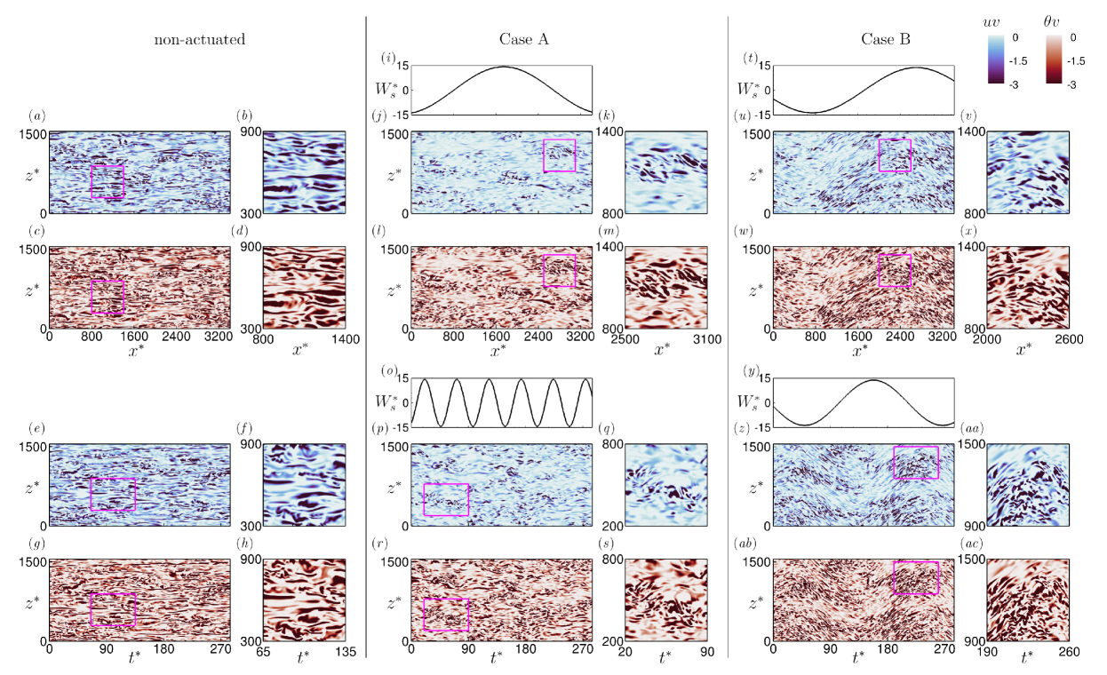
Figure 16: Visualisations of the instantaneous fields of $uv$ (blue intensity fields) and $\theta v$ (brick intensity fields) at $y^{+}=14$ for the same cases as in figure 15. Next to each field, we magnify the small square outlined in pink. Left: non-actuated case; middle: actuated Case A; right: actuated Case B. The top two rows visualise $uv$ and $\theta v$ at one time over the $x^{*}$-$z^{*}$ plane. (i,t) plot the corresponding spanwise wall velocity $W^{*}_{s}$ over $x^{*}$ at the same time. The bottom two rows visualise $uv$ and $\theta v$ at one $x^{*}$-location over $z^{*}$ and time $t^{*}$. (o,y) plot $W^{*}_{s}$ over $t^{*}$ at the same $x^{*}$-location.

At a fixed $\omega^{+}$, $uv$ and $\theta v$ are exposed to an identical Stokes layer. However, the larger change in $\Delta k^{*}_{x}\phi^{*}_{\theta v}$ compared to $\Delta k^{*}_{x}\phi^{*}_{uv}$ for $Pr>1$ implies that $\theta v$ is locally exposed to a stronger Stokes layer production than $uv$. We establish this connection by evaluating the Stokes layer production $P^{*}_{33p}$ at the origin of turbulence in $uv$ and $\theta v$, namely at the peaks in the non-actuated $k^{*}_{x}\phi^{*}_{uv_{0}}$ and $k^{*}_{x}\phi^{*}_{\theta v_{0}}$. Figure 17(a) demonstrates this process at $Pr=7.5$; note that the $(y^{*},\lambda^{*}_{x})$ axes are inverted compared to the plots in figure 15. With increasing $Pr$, the conductive sublayer thins, and the peak in $\Delta k^{*}_{x}\phi^{*}_{\theta v_{0}}$ moves closer to the wall compared to the peak in $\Delta k^{*}_{x}\phi^{*}_{uv_{0}}$. As a result, at each $\omega^{+}$ the origin of turbulence in $\theta v$ is locally exposed to a larger Stokes layer production compared to $uv$. This in turn drops $I_{\theta v}$ below $I_{uv}$. We demonstrate this in figure 17(b). At $Pr=0.71$, $I_{\theta v}$ and $I_{uv}$ are exposed to similar levels of $P^{*}_{33p}$, but at higher Prandtl numbers $I_{\theta v}$ is exposed to an order of magnitude larger production. In addition, at $\omega^{+}=0.022$ $I_{\theta v}$ is exposed to a significantly larger $P^{*}_{33p}$ than at $\omega^{+}=0.110$. As a result, the exponent $\gamma$ increases from $\gamma=0.11$ ($\omega^{+}=0.11$) to $0.53$ ($\omega^{+}=0.022$).

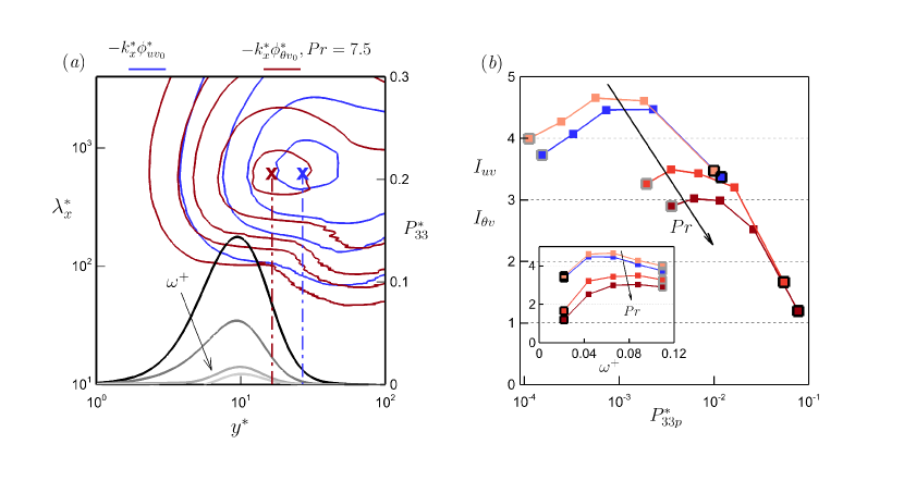
Figure 17: Assessment of the relation between $I_{uv}$ and $I_{\theta v}$, and the local Stokes layer production $P^{*}_{33p}$ at the peaks in the non-actuated $k^{*}_{x}\phi^{*}_{uv_{0}}$ and $k^{*}_{x}\phi^{*}_{\theta v_{0}}$. (a) Illustrates obtaining of $P^{*}_{33p}$ for $k^{*}_{x}\phi^{*}_{uv_{0}}$ (blue contour lines) and $k^{*}_{x}\phi^{*}_{\theta v_{0}}$ at $Pr=7.5$ (brick red contour lines), by intersecting their peaks with the $P^{*}_{33}$ profiles (black to grey lines); the contour levels change from $0.02$ to $0.047$ with an increment of $0.075$. (b) Same data of $I_{uv}$ and $I_{\theta v}$ as in figure 14(c), but versus $P^{*}_{33p}$; to ease the inspection, the inset shows figure 14(c). The data points at $\omega^{+}=0.022$ and $0.110$ have black and grey outlines, respectively.

We have seen how the behaviour of the Stokes layer leads to $I_{\theta v}<I_{uv}$ by examining the streamwise and frequency spectrograms. This connection is more difficult to find in the spanwise spectrograms $k^{*}_{z}\phi^{*}_{uv}$ and $k^{*}_{z}\phi^{*}_{\theta v}$ (figures 15i–l, u–x). The Stokes layer predominantly modifies the time scale $T^{*}$, hence the streamwise length-scale $\lambda^{*}_{x}$, of the near-wall turbulence. However, $k^{*}_{z}\phi^{*}_{uv}$ and $k^{*}_{z}\phi^{*}_{\theta v}$ are integrated over $T^{*}$ and $\lambda^{*}_{x}$, and so the smaller-scale energy amplification is cancelled by the large-scale energy attenuation. Thus, even though the Stokes layer protrusion (production) increases from Case A to Case B, the distributions of $k^{*}_{z}\phi^{*}_{uv}$ and $k^{*}_{z}\phi^{*}_{\theta v}$ suggest that the near-wall turbulence is distorted to a lesser extent.

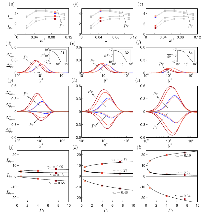
Figure 18: Large- and small-scale contributions to $\Delta^{*}_{uv},\Delta^{*}_{\theta v}$ and their integrals $I_{uv},I_{\theta v}$ for the travelling wave case. Left column $\omega^{+}=0.088$; middle $\omega^{+}=0.044$; right $\omega^{+}=0.022$. Blue $uv$ profiles; for $\theta v$ profiles light orange $Pr=0.71$, orange 4.0, brick red 7.5. (a,b,c) $I_{uv},I_{\theta v}$ versus $\omega^{+}$. (d,e,f) $\Delta^{*}_{uv},\Delta^{*}_{\theta v}$ versus $y^{*}$; the insets plot $\overline{\tilde{w}^{2}}^{*}$ representing the Stokes layer where the bold number reports $\ell^{*}_{0.01}$. (d,e,f) Total $\Delta^{*}_{uv}\Delta^{*}_{\theta v}$; (g,h,i) decomposed $\Delta^{*}_{uv\pm},\Delta^{*}_{\theta v\pm}$. (j,k,l) Total $I_{\theta v}$ and decomposed $I_{\theta v}\pm$ versus $Pr$. Solid curves: $I_{\theta v\pm}=Pr^{\gamma\pm}I_{uv\pm}$ and $I_{\theta v}=Pr^{-\gamma}I_{uv}$ (thicker line).

Our observations regarding the large-scale attenuation and small-scale amplification can be extended by applying scale-wise decomposition to $\Delta^{*}_{uv}$ and $\Delta^{*}_{\theta v}$. For instance, we can write $\Delta^{*}_{uv}=\Delta^{*}_{uv+}+\Delta^{*}_{uv-}$, where

$$\Delta^{*}_{uv+} =\int_{\lambda^{*}_{x}>350}\Delta\phi^{*}_{uv}(k^{*}_{x},y^{*})dk^{*}_{x}-y^{*}\left(Re^{-1}_{\tau}-Re^{-1}_{\tau_{0}}\right),$$ (3.8a)

$$\Delta^{*}_{uv-} =\int_{\lambda^{*}_{x}\leq 350}\Delta\phi^{*}_{uv}(k^{*}_{x},y^{*})dk^{*}_{x}.$$ (3.8b)

We set the threshold of $\lambda^{*}_{x}=350$ for partitioning because the spectrograms for all cases show $\Delta k^{*}_{x}\phi^{*}_{uv}>0$ for $\lambda^{*}_{x}\gtrsim 350$, and $\Delta k^{*}_{x}\phi^{*}_{uv}<0$ for $\lambda^{*}_{x}\lesssim 350$ (see figures 15e,q). As noted earlier (figure 9a and 3.3a), we need to subtract the term $y^{*}\left(Re^{-1}_{\tau}-Re^{-1}_{\tau_{0}}\right)$ from $\Delta\overline{uv}^{*}$ to obtain its net contribution $\Delta^{*}_{uv}$. Considering figure 15(e,q), this contribution appears in the large scales of $\Delta k^{*}_{x}\phi^{*}_{uv}$ ($\lambda^{*}_{x}>350$), and therefore we subtract $y^{*}\left(Re^{-1}_{\tau}-Re^{-1}_{\tau_{0}}\right)$ from the large-scale integration (3.8a). The same reasoning is applied to the partitioning of $\Delta^{*}_{\theta v}$, and we calculate $\Delta^{*}_{\theta v+}$ and $\Delta^{*}_{\theta v-}$ in a manner that is identical to that expressed by (3.8a) and (3.8b).

We show these decompositions in figure 18 for the travelling wave actuation as $\omega^{+}$ varies from 0.088 to 0.022. We see that increasing the protrusion of the Stokes layer simultaneously increases the large-scale attenuation ($\Delta^{*}_{uv+}$ and $\Delta^{*}_{\theta v+}$ become more positive) and the small-scale amplification ($\Delta^{*}_{uv-}$ and $\Delta^{*}_{\theta v-}$ become more negative). At $Pr=0.71$, as $\omega^{+}$ changes from 0.088 to the optimal value of 0.044, $\Delta^{*}_{uv+}$ and $\Delta^{*}_{\theta v+}$ are amplified slightly more than $\Delta^{*}_{uv-}$ and $\Delta^{*}_{\theta v-}$, leading to the increase in $I_{uv}$ and $I_{\theta v}$. However, as $\omega^{+}$ changes from 0.044 to 0.022, this trend is reversed and we see a decrease in $I_{uv}$ and $I_{\theta v}$. At $Pr=4.0$ and 7.5, from the optimal $\omega^{+}=0.088$ to the sub-optimal $\omega^{+}=0.022$, $\Delta^{*}_{\theta v-}$ is amplified more than $\Delta^{*}_{\theta v+}$, leading to the reduction in $I_{\theta v}$. At these Prandtl numbers, the decomposition is significantly modified from an asymmetric distribution at $\omega^{+}=0.088$ ($\Delta^{*}_{\theta v+}>\Delta^{*}_{\theta v-}$) to an almost symmetric distribution at $\omega^{+}=0.022$ ($\Delta^{*}_{\theta v+}\simeq\Delta^{*}_{\theta v-}$).

In figures 18(j,k,l), we plot the integrals $I_{\theta v}$, $I_{\theta v+}$, and $I_{\theta v-}$. At each value of $\omega^{+}$, $I_{\theta v+}$ becomes more positive and $I_{\theta v-}$ becomes more negative with increasing $Pr$. By fitting the power-laws $I_{\theta v\pm}=Pr^{\gamma\pm}I_{uv\pm}$ to the data, we find that at each $\omega^{+}$, $\gamma-$ is $2$ to $7$ times larger than $\gamma+$. In other words, small-scale amplification ($I_{\theta v-}$) grows with a higher power of $Pr$ than large-scale attenuation ($I_{\theta v+}$), leading to the decay of $I_{\theta v}$ with $Pr$. As discussed with respect to figure 17, the faster growth rate of $I_{\theta v-}$ compared to $I_{\theta v+}$ with increasing $Pr$ is due to the thinning of the conductive sublayer and the exposure of the near-wall thermal field to higher Stokes layer production.

3.8 Comparison between the travelling wave and the plane oscillation

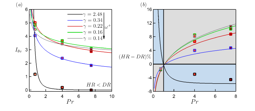
Figure 19: Similar plots as in figure 11(b,d), but for the plane oscillation with $A^{+}=12$ (figure 3c). The outline colour of each data point indicates its $\omega^{+}$; $\omega^{+}=0.022$ (black), $0.044$ (blue), $0.066$ (red), $0.088$ (green) and $0.110$ (grey).

All our findings based on the travelling wave motion (§3.3 to §3.7) remain broadly valid for the case of plane oscillation. By comparing figures 19 and 20 with figures 11 and 14, we see that, for example, the power-law relation $I_{\theta v}=I_{uv}/Pr^{\gamma}$ fits well with the plane oscillation data (figure 19a), and the division $HR>DR$ ($\gamma<0.5$) and $HR<DR$ ($\gamma>0.5$) is also valid (figures 19b). The value of $\gamma$ at each $\omega^{+}$ is close to its counterpart for the travelling wave case, with the exception of $\omega^{+}=0.022$, where $\gamma=2.48$ for the plane oscillation (black lines in figure 19), almost five times larger the the value of 0.53 found for the travelling wave motion. Such a strong decay rate drops $I_{\theta v}$ to almost zero by $Pr=7.5$ for the plane oscillation, leading to $HR-DR\simeq-5\%$. This strong decay is associated with the appearance of a highly protrusive Stokes layer (figures 20a,c), in agreement with the discussion given in §3.7.

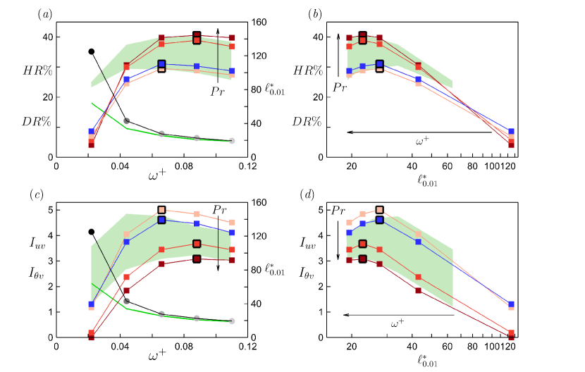
Figure 20: Same plots as in figure 14, except the data points (filled squares and circles) are from the plane oscillation with $A^{+}=12$. The range of variations in the travelling wave data points are shaded in green. In (a,c), the green lines plot $\ell^{*}_{0.01}$ versus $\omega^{+}$ for the travelling wave.

Figure 20 shows that for $0.066\leq\omega^{+}\leq 0.110$, $DR$, $HR$, $I_{uv}$, $I_{\theta v}$, and $\ell^{*}_{0.01}$ for the plane oscillation are close to the values found for the travelling wave. However, as $\omega^{+}$ decreases to $0.044$ and then to $0.022$, significant differences appear. For the plane oscillation, the Stokes layer becomes highly protrusive, reaching up to $\ell^{*}_{0.01}\simeq 120$ at $\omega^{+}=0.022$. As discussed in §3.7, such a protrusive Stokes layer loses its efficacy in producing a net attenuation of the near-wall turbulence. As a result, $I_{uv}$ and $I_{\theta v}$ significantly drop, and $\gamma$ rises significantly. Rouhi et al. (2023) showed that when $\ell^{*}_{0.01}\sim\mathcal{O}(10^{2})$, the Stokes layer departs from its laminar-like structure, the mean velocity and temperature profiles become highly disturbed (figure 25j,k,l), and the predictive relations for $DR$ (3.5a) and $HR$ (3.5b) begin to fail. Similarly, we observe that at $\omega^{+}=0.022$ the predictive relation for $HR$ (3.5b) is much less accurate compared to its performance at higher frequencies (figure 19b).

As a final note, it appears that $\gamma$, a $Pr$-independent quantity, increases almost linearly with $\ell^{*}_{0.01}$ and $P^{*}_{{33}_{\mathrm{max}}}$, and decreases inversely with increasing $\omega^{+}$ following

$$\gamma\simeq 4.2P^{*}_{{33}_{\mathrm{max}}}\simeq 0.008\ell^{*}_{0.01}\simeq{1}/{80\omega^{+}}.$$ (3.9)

This is supported by the results shown in figure 21, where we compile all our data for the travelling wave and the plane oscillation cases (with the exception of the plane oscillation at $\omega^{+}=0.022$ where the Stokes layer is particularly protrusive).

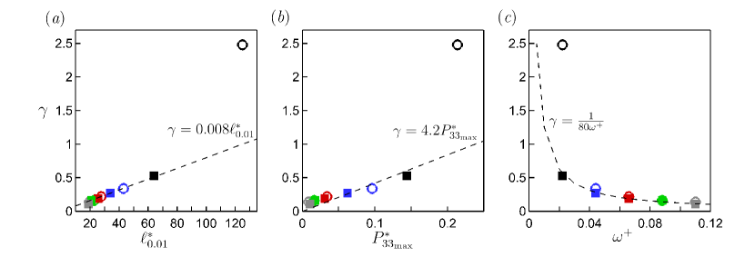
Figure 21: Assessment of the relations (3.9) between $\gamma$, $P^{*}_{33_{\mathrm{max}}}$, $\ell^{*}_{0.01}$ and $\omega^{+}$ for the travelling wave (filled squares) and the plane oscillation (empty circles); $\omega^{+}=0.022$ (black), $0.044$ (blue), $0.066$ (red), $0.088$ (green) and $0.110$ (grey).

4 Conclusions

Direct numerical simulations of turbulent (open) channel flow with forced convection were performed at a friction Reynolds number of 590 for Prandtl numbers of 0.71 (air), 4.0, 7.5 (water), and 20 (molten salt). Spanwise wall forcing was applied either as a plane wall oscillation or a streamwise in-plane travelling wave with wavenumber $\kappa^{+}_{x}=0.0014$ ($\lambda^{+}\simeq 4500$). For both oscillation mechanisms, we fix the amplitude $A^{+}=12$ and change the frequency from $\omega^{+}=0.022$ to $0.110$ (upstream travelling waves only). These frequencies are restricted to the inner-scaled actuation pathway (Marusic et al., 2021; Chandran et al., 2023).

The key finding of the present work is that for $Pr\gtrsim 4.0$ and $\omega^{+}\gtrsim 0.044$, $HR$ exceeds $DR$, that is, the Reynolds analogy no longer holds. Under these conditions, $HR\approx 40\%$ and $DR\approx 30\%$. This result applies to the travelling wave motion and the plane oscillation. To help understand this result, we derived explicit relations between $HR$ and $DR$ and the integrals of the attenuation in the turbulent shear-stress ($I_{uv}$) and turbulent temperature-flux ($I_{\theta v}$). For the cases considered here, we find that $I_{\theta v}\simeq I_{uv}/Pr^{\gamma}$, where $\gamma$ depends inversely on $\omega^{+}$. We arrive at $HR-DR\propto Pr^{(0.5-\gamma)}-1$. Thus, $HR\simeq DR$ when $\gamma=0.5$, and for $Pr>1$, $HR>DR$ ($HR<DR$) when $\gamma<0.5$ ($\gamma>0.5$). The travelling wave and the plane oscillation perform similarly from $\omega^{+}=0.044$ ($\gamma\simeq 0.3$) to $0.110$ ($\gamma\simeq 0.1$), where $HR-DR$ increases from $5\%$ to $10\%$ at $Pr=7.5$. However, at $\omega^{+}=0.022$, the travelling wave and plane oscillation cases differ, owing to their different Stokes layer structure. At this frequency, for the travelling wave motion $\gamma\simeq 0.5$, corresponding to $HR\simeq DR$ at all values of $Pr$, while for the plane oscillation $\gamma\simeq 2.5$, corresponding to $HR-DR\simeq-5\%$ at $Pr=7.5$.

Breaking the analogy between $I_{uv}$ and $I_{\theta v}$ for $Pr\neq 1$ is related to their different responses to the Stokes layer. The Stokes layer modifies the energy distribution among the scales of $uv$ and $\theta v$ in two counteracting ways; 1) it favourably attenuates the energy of the large scales with streamwise length scales $\lambda^{*}_{x}\gtrsim 350$ and time scales $T^{*}\gtrsim 35$, and 2) it unfavourably amplifies the energy of the small scales with $\lambda^{*}_{x}\lesssim 350,T^{*}\lesssim 35$. When the Prandtl number increases and the conductive sublayer thins, the energetic scales of $\theta v$ move closer to the wall, where they are exposed to a stronger Stokes layer production than the energetic scales of $uv$. By increasing the Stokes layer production, the small-scale energy amplification increases more than the large-scale energy attenuation, and so $I_{\theta v}$ drops below $I_{uv}$.

The time scale of the near-wall energetic temperature scales $\mathcal{T}^{+}_{\theta}$ was found to be almost insensitive to $Pr$, and it remains close to its counterpart for the velocity scales $\mathcal{T}^{+}_{u}\simeq 100$. As a result, for the plane oscillation, the optimal value of $\omega^{+}$ for the maximum $HR$ is close to the one for the maximum $DR$, that is, $\omega^{+}\simeq 2\pi/100\simeq 0.066$. However, for the travelling wave, the optimal frequency for $HR$ changes from $0.044$ at $Pr=0.71$ to $0.088$ at $Pr=7.5$ because it depends on the advection speed of the energetic temperature scales. The thinning of the conductive sublayer decreases the advection speed, and so the optimal frequency of actuation increases.

From the Prandtl number scaling of the thermal statistics, we derived a predictive model for $HR$. By knowing $\gamma$ and $I_{uv}$ for a fixed set of actuation parameters $(A^{+},\kappa^{+}_{x},\omega^{+})$ at a given Reynolds and Prandtl number, the model predicts $HR$ at other Prandtl and Reynolds numbers. Using this model, we generated a map $HR(Pr,Re_{\tau_{0}})$ for the optimal case with $\omega^{+}=0.088$, and found good agreement with the computations for Prandtl numbers up to 7.5. To further evaluate the model, we conducted an extra simulation at $\omega^{+}=0.088$ and $Pr=20,Re_{\tau_{0}}=590$. Again, good agreement with the model was found (model $HR=43\%,HR-DR=13\%$ compared with DNS $HR=45\%,HR-DR=14\%$).

Acknowledgements
The research was funded through the Deep Science Fund of Intellectual Ventures (IV). We acknowledge Dr. Daniel Chung for providing his DNS solver. We thank EPSRC for the computational time made available on ARCHER2 via the UK Turbulence Consortium (EP/R029326/1), and IV for providing additional computational time on ARCHER2.

Declaration of interests. The authors report no conflict of interest.

Appendix A Validation of the grid and the domain size

The production runs were performed in a reduced-domain channel flow ($L_{x}\gtrsim 2.7h,L_{z}\simeq 0.85h$) with grid resolution $\Delta^{+}_{x}\times\Delta^{+}_{z}\simeq 8\times 4$; we call this setup “reduced coarse”. To check that this setup gives accurate $DR,HR$ and statistics of interest over our parameter space, calculations with a finer grid resolution of $\Delta^{+}_{x}\times\Delta^{+}_{z}\simeq 4\times 2$ were conducted in a full-domain channel flow ($L_{x}\gtrsim 2\pi h,L_{z}\simeq\pi h$); we call this setup “full fine”. Two additional setups are also used, called “full coarse” ($L_{x}\gtrsim 7.6h,L_{z}\simeq\pi h,\Delta^{+}_{x}\times\Delta^{+}_{z}\simeq 8\times 4$) and “full intermediate” ($L_{x}\gtrsim 7.6h,L_{z}\simeq\pi h,\Delta^{+}_{x}\times\Delta^{+}_{z}\simeq 6\times 3$). For all simulations, $Re_{\tau_{0}}=590$ and $A^{+}=12$. For all the reduced domain cases, we reconstruct the $\overline{U}^{*}$ and $\overline{\Theta}^{*}$ profiles beyond $y^{*}_{\mathrm{res}}=170$, and calculate $DR$ and $HR$ following our approach in §2.3.

For the non-actuated channel flow at $Pr=7.5$, table 2 shows that for the full fine and reduced coarse setups, the Nusselt numbers $Nu_{0}$ are identical, and the skin-friction coefficients $C_{f_{0}}$ differ by less than $2\%$. The profiles of $\overline{\Theta}^{+}$ and $\overline{\theta^{2}}^{+}$ are also in excellent agreement (figure 22). The small differences between our results and those from the DNS of Alcántara-Ávila & Hoyas (2021) are most likely due to the differences in $Re_{\tau_{0}}$ and $Pr$ (590 compared to 500, and 7.5 compared to 7).

setup	$Re_{\tau_{0}}$	$Pr$	$L_{x},L_{z}$	$\Delta^{+}_{x}\times\Delta^{+}_{z}$	$C_{f_{0}}$	$Nu_{0}$	Legend
full fine	$590$	$7.5$	$2\pi h,\pi h$	$3.6\times 1.8$	$0.0058$	$162$
reduced coarse	$590$	$7.5$	$2.7h,0.85h$	$8.3\times 3.9$	$0.0057$	$162$
Alcántara-Ávila & Hoyas (2021)	$500$	$7.0$	$2\pi h,\pi h$	$8.2\times 4.1$	-	$132$

Table 2: Validation simulations for the reduced coarse setup. Non-actuated channel flow at $Pr=7.5$. Statistics for these cases are shown in figure 22.

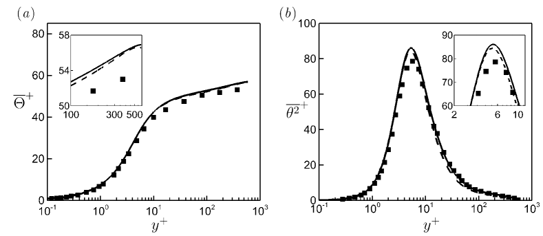
Figure 22: Comparing the results for the three setups given in table 2. (a) Mean temperature profiles $\overline{\Theta}^{+}$. (b) Mean square of turbulent temperature $\overline{\theta^{2}}^{+}$ . Solid line, “full fine” setup. Dashed line: “reduced coarse” setup. Square symbols: reference DNS of Alcántara-Ávila & Hoyas (2021).

case	$Pr$	$\kappa^{+}_{x}$	$\omega^{+}$	$L_{x},L_{z}$	$\Delta^{+}_{x}\times\Delta^{+}_{z}$	$DR\%$	$HR\%$
full coarse	$0.71$	$0.0014$	$0.022$	$7.6h,\pi h$	$7.4\times 3.9$	$24.5$	$23.3$
reduc. coarse	$0.71$	$0.0014$	$0.022$	$7.6h,0.85h$	$8.8\times 3.9$	$25.2$	$23.6$		Set 1
full coarse	$0.71$	$0.0014$	$0.044$	$7.6h,\pi h$	$7.4\times 3.9$	$30.4$	$29.1$		${\epsilon_{DR}}_{\mathrm{max}},{\epsilon_{HR}}_{\mathrm{max}}$
reduc. coarse	$0.71$	$0.0014$	$0.044$	$7.6h,0.85h$	$8.8\times 3.9$	$30.6$	$29.3$		$0.7\%,0.6\%$
full coarse	$0.71$	$0.0014$	$0.088$	$7.6h,\pi h$	$7.4\times 3.9$	$29.9$	$28.5$
reduc. coarse	$0.71$	$0.0014$	$0.088$	$7.6h,0.85h$	$8.8\times 3.9$	$29.3$	$27.9$
								Legends
full fine		$0.0014$	$0.022$	$7.6h,\pi h$	$3.9\times 1.8$	$26.2$	$25.4$
reduc. coarse		$0.0014$	$0.022$	$7.6h,0.85h$	$8.8\times 3.9$	$25.6$	$24.0$
									Set 2
full fine		$0.0014$	$0.044$	$7.6h,\pi h$	$3.9\times 1.8$	$31.4$	$38.6$
full inter.	${\epsilon_{DR}}_{\mathrm{max}},{\epsilon_{HR}}_{\mathrm{max}}$	$0.0014$	$0.044$	$7.6h,\pi h$	$5.8\times 2.7$	$30.9$	$37.7$
full coarse	$7.5$	$0.0014$	$0.044$	$7.6h,\pi h$	$8.8\times 4.0$	$31.0$	$37.0$		$1.5\%,1.6\%$
reduc. coarse		$0.0014$	$0.044$	$7.6h,0.85h$	$8.8\times 3.9$	$31.8$	$37.7$
full fine		$0.0014$	$0.088$	$7.6h,\pi h$	$3.9\times 1.8$	$29.0$	$39.8$
reduc. coarse		$0.0014$	$0.088$	$7.6h,0.85h$	$8.8\times 3.9$	$30.5$	$40.4$
full fine	$7.5$	$0$	$0.044$	$2\pi h,\pi h$	$3.6\times 1.8$	$25.2$	$28.9$		Set 3
reduc. coarse	$7.5$	$0$	$0.044$	$2.7h,0.85h$	$8.3\times 3.9$	$26.5$	$30.8$
									${\epsilon_{DR}}_{\mathrm{max}},{\epsilon_{HR}}_{\mathrm{max}}$
full fine	$7.5$	$0$	$0.088$	$2\pi h,\pi h$	$3.6\times 1.8$	$29.4$	$39.0$		$1.4\%,1.9\%$
reduc. coarse	$7.5$	$0$	$0.088$	$2.7h,0.85h$	$8.3\times 3.9$	$30.8$	$40.7$

Table 3: Validation simulations for grid and domain size.

For the actuated channel flow cases at $Pr=0.71$ and $7.5$, table 3 lists three sets of validation cases. For Set 1, we compare the “reduced coarse” setup with the “full coarse” setup because the grid resolution of $\Delta^{+}_{x}\times\Delta^{+}_{z}\simeq 8\times 4$ is fine enough at this $Pr$ (Pirozzoli et al., 2016; Alcántara-Ávila et al., 2018, 2021; Alcántara-Ávila & Hoyas, 2021). Sets 1 and 2 are travelling wave cases, and Set 3 is for the plane oscillation case. For each set, we see that reducing the domain size and coarsening the grid from the full fine setup to the reduced coarse setup changes $DR$ and $HR$ by a maximum of $1.5\%$ and $1.9\%$, respectively.

Set 2 contains the most challenging cases over the range $0.71\leq Pr\leq 7.5$ in terms of their grid resolution requirement. In figure 23, we compare the mean temperature $\overline{\Theta}^{*}$ profiles for $Pr=7.5$. Excellent agreement is obtained between the full fine setup and the reduced coarse setup at $\omega^{+}=0.022$ and $0.088$ (figures 23a,c). At $\omega^{+}=0.044$, there is some sensitivity to the grid, where at $y^{*}=200$, $\overline{\Theta}^{*}=74.3$ for the full fine setup, and 73.0 for the reduced coarse setup. This difference (1.3 units) is small relative to the temperature difference $\Delta\overline{\Theta}^{*}_{200}\simeq 19.0$ between the actuated and the non-actuated profiles. In figure 24, we assess the accuracy of the reduced coarse setup in resolving $\overline{\theta^{2}}^{*}$, $k^{*}_{x}\phi^{*}_{\theta\theta}$, and $\ k^{*}_{z}\phi^{*}_{\theta\theta}$ at $\omega^{+}=0.044$. The reduced coarse setup results agree well with the full fine setup results, especially in matching the energetic peaks in $k^{*}_{x}\phi^{*}_{\theta\theta}$ and $\ k^{*}_{z}\phi^{*}_{\theta\theta}$ in magnitude, location, and length scales $\lambda^{*}_{x},\lambda^{*}_{z}$.

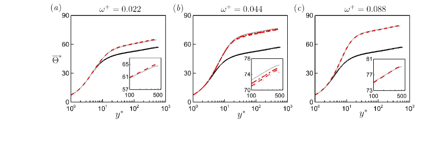
Figure 23: Comparison of the mean temperature profiles for the travelling wave at $Pr=7.5$ (Set 2, table 3). (a) $\omega^{+}=0.022$, (b) $\omega^{+}=0.044$ and (c) $\omega^{+}=0.088$. Solid grey line: “full fine” case. Dashed-dotted red line: “full inter.” case. Dotted red line: full coarse case. Dashed red line:“reduc. coarse” case. Solid black line: non-actuated “full fine” case.

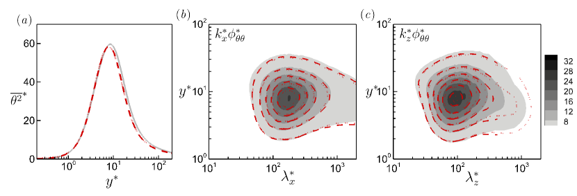
Figure 24: Comparison of (a) mean square of turbulent temperature $\overline{\theta^{2}}^{*}$, and (b,c) pre-multiplied streamwise and spanwise spectrograms $k^{*}_{x}\phi^{*}_{\theta\theta},k^{*}_{x}\phi^{*}_{\theta\theta}$ for the travelling wave at $Pr=7.5$, $\omega^{+}=0.044$ (Set 2, table 3). Solid grey line and grey-scale contour field: “full fine” case. Dotted red line and dotted contour lines: “full coarse” case. Dashed red line and dashed contour lines:“reduc. coarse” case.

case	$Pr$	$\kappa^{+}_{x}$	$\omega^{+}$	$L_{x},L_{z}$	$\Delta^{+}_{x}\times\Delta^{+}_{z}$	$C_{f_{0}}$	$C_{h_{0}}$	$DR\%$	$HR\%$
reduc. coarse	$20.0$	-	-	$2.7h,0.85h$	$8.3\times 3.9$	$0.0057$	$5.47\times 10^{-4}$	-	-
reduc. inter.	$20.0$	-	-	$2.7h,0.85h$	$6.2\times 2.6$	$0.0057$	$5.44\times 10^{-4}$	-	-
reduc. coarse	$20.0$	$0.0014$	$0.088$	$7.6h,0.85h$	$8.8\times 3.9$	-	-	$29.5$	$43.5$
reduc. inter.	$20.0$	$0.0014$	$0.088$	$7.6h,0.85h$	$5.8\times 2.6$	-	-	$28.6$	$43.1$

Table 4: Validation cases at $Re_{\tau_{0}}=590$ and $Pr=20.0$.

Table 4 summarises our validation study at $Pr=20.0$ (table 1). For the non-actuated case (table 4), $C_{f_{0}}$ and $C_{h_{0}}$ from the coarse grid results differ from the intermediate grid results by a maximum of $0.5\%$, and for the travelling wave case, $DR$ and $HR$ differ by $<1\%$.

Based on these results, we conclude that $DR,HR$ and the statistics of interest can be accurately computed using the reduced coarse setup with the grid resolution of $\Delta^{+}_{x}\times\Delta^{+}_{z}\simeq 8\times 4$, and the domain size of $L_{x}\times L_{z}\simeq 7.6h\times 0.85h$ for the travelling wave case ($\kappa^{+}_{x}=0.0014$), and the domain size of $L_{x}\times L_{z}\simeq 2.7h\times 0.85h$ for the plane oscillation case ($\kappa^{+}_{x}=0$). These grid and domain size prescriptions were used for our production calculations (table 1).

Appendix B Relation between heat-transfer reduction and temperature difference

The mean velocity $\overline{U}^{*}$ and temperature $\overline{\Theta}^{*}$ profiles in the log region and beyond can be expressed based on the following semiempirical wall-wake relations (Rouhi et al., 2022)

$$\overline{U}^{*} =\frac{1}{\kappa_{u}}\ln(y^{*})+B_{u}+\frac{2\Pi_{u}}{\kappa_{u}}\mathcal{W}_{u}(y/h)+\Delta\overline{U}^{*}_{\mathrm{log}},$$ (C1a)

$$\overline{\Theta}^{*} =\frac{1}{\kappa_{\theta}}\ln(y^{*})+B_{\theta}+\frac{2\Pi_{\theta}}{\kappa_{\theta}}\mathcal{W}_{\theta}(y/h)+\Delta\overline{\Theta}^{*}_{\mathrm{log}},$$ (C1b)

where $\kappa_{u},\kappa_{\theta}$ and $B_{u}$ are constants, but the offset $B_{\theta}$ depends on $Pr$ (Kader & Yaglom, 1972; Kader, 1981). The wake profiles $(2\Pi_{u}/\kappa_{u})\mathcal{W}_{u}(y/h)$ and $(2\Pi_{\theta}/\kappa_{\theta})\mathcal{W}_{\theta}(y/h)$ depend on the flow configuration, e.g. channel, pipe or boundary layer (Pope, 2000; Nagib & Chauhan, 2008). The log-law shifts, $\Delta\overline{U}^{*}_{\mathrm{log}}$ and $\Delta\overline{\Theta}^{*}_{\mathrm{log}}$, are non-zero for the actuated cases. These log-law shifts are evaluated at $y^{*}=170$, where $\Delta\overline{U}^{*}$ and $\Delta\overline{\Theta}^{*}$ approximately reach their asymptotic values (figures 4 and 7). For fixed operating parameters ($A^{+},\kappa^{+}_{x},\omega^{+}$), $\Delta\overline{U}^{*}_{\mathrm{log}}$ is constant for the upstream travelling wave  (Hurst et al., 2014; Gatti & Quadrio, 2016; Rouhi et al., 2023). However, $\Delta\overline{\Theta}^{*}_{\mathrm{log}}$ strongly depends on $Pr$ (figures 7k,l). We set the constants $\kappa_{u}=0.4$, $\kappa_{\theta}=0.46$ and $B_{u}=5.2$ following Pirozzoli et al. (2016) and Rouhi et al. (2022), and obtain the offset $B_{\theta}(Pr)=12.5Pr^{2/3}+2.12\ln Pr-5.3$ following Kader & Yaglom (1972), which is reported to be accurate for $Pr\gtrsim 0.7$. The suitability of these choices is confirmed in §2.3 and Appendix A.

The bulk velocity $U^{*}_{b}$ and bulk temperature $\Theta^{*}_{b}$ are found by integrating (C1a) and (C1b), so that

$$U^{*}_{b} =\frac{1}{\kappa_{u}}\ln(Re_{\tau})-\frac{1}{\kappa_{u}}+B_{u}+\frac{2\Pi_{u}}{\kappa_{u}}\int_{0}^{h}\mathcal{W}_{u}(y/h)dy+\Delta\overline{U}^{*}_{\mathrm{log}},$$ (C2a)

$$\Theta^{*}_{b} =\frac{1}{\kappa_{\theta}}\ln(Re_{\tau})-\frac{1}{\kappa_{\theta}}+B_{\theta}+\frac{2\Pi_{\theta}}{\kappa_{\theta}}\int_{0}^{h}\mathcal{W}_{\theta}(y/h)dy+\Delta\overline{\Theta}^{*}_{\mathrm{log}}.$$ (C2b)

By subtracting the non-actuated $U^{*}_{b_{0}}$ and $\Theta^{*}_{b_{0}}$ from their actuated counterparts $U^{*}_{b}$ and $\Theta^{*}_{b}$, and by assuming that the wake profiles are not influenced by the wall oscillation, we obtain

$$U^{*}_{b}-U^{*}_{b_{0}}=\frac{1}{\kappa_{u}}\ln\left(\frac{Re_{\tau}}{Re_{\tau_{0}}}\right)+\Delta\overline{U}^{*}_{\mathrm{log}},\qquad\Theta^{*}_{b}-\Theta^{*}_{b_{0}}=\frac{1}{\kappa_{\theta}}\ln\left(\frac{Re_{\tau}}{Re_{\tau_{0}}}\right)+\Delta\overline{\Theta}^{*}_{\mathrm{log}}.$$ (C3a,b)

When $Re_{\tau}$ is matched between the actuated and the non-actuated cases ($Re_{\tau}=Re_{\tau_{0}}$), the first term on the right-hand-side of (C3a,b) disappears. However, when the bulk Reynolds number $Re_{b}$ is matched, as in our work, this term is retained because $Re_{\tau}\neq Re_{\tau_{0}}$. By using (C3a,b) and the relations $C_{f}=2/{U^{*}_{b}}^{2},\ C_{h}=1/(U^{*}_{b}\Theta^{*}_{b}),\ C_{f}/C_{f_{0}}=R_{f}=1-DR$, and $C_{h}/C_{h_{0}}=R_{h}=1-HR$, we can relate $\Delta\overline{U}^{*}_{\mathrm{log}}$ and $\Delta\overline{\Theta}^{*}_{\mathrm{log}}$ to $R_{f}$ and $R_{h}$ according to

$$\Delta\overline{U}^{*}_{\mathrm{log}} =\sqrt{\frac{2}{C_{f_{0}}}}\left[\frac{1}{\sqrt{R_{f}}}-1\right]-\frac{1}{2\kappa_{u}}\ln R_{f},$$ (C4a)

$$\Delta\overline{\Theta}^{*}_{\mathrm{log}} =\frac{\sqrt{C_{f_{0}}/2}}{C_{h_{0}}}\left[\frac{\sqrt{R_{f}}}{R_{h}}-1\right]-\frac{1}{2\kappa_{\theta}}\ln R_{f}.$$ (C4b)

Equation (C4a) was first derived by Gatti & Quadrio (2016) (their equation 4.7). Equation (C4b) is new.

Appendix C Statistics for the plane oscillation

See figures 25 and 26.

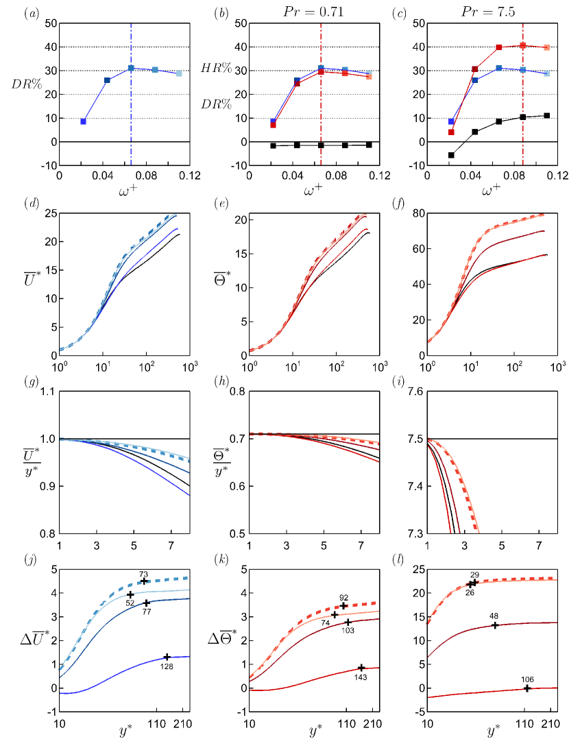
Figure 25: Same plots as in figure 7, but for the plane oscillation case with $A^{+}=12$.

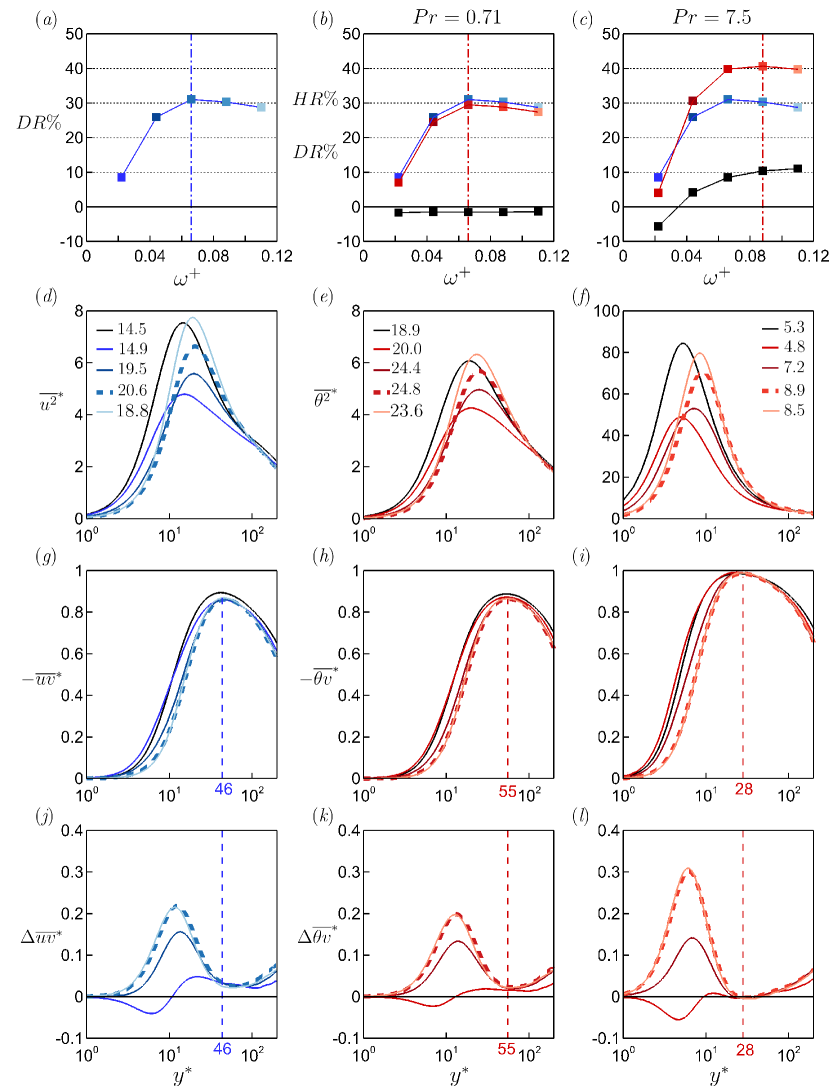
Figure 26: Same plots as in figure 8, but for the plane oscillation case with $A^{+}=12$.