justified
A spin chain with non-Hermitian symmetric boundary couplings: exact solution, dissipative Kondo effect, and phase transitions on the edge
Abstract
We construct an exactly solvable symmetric non-Hermitian model where a spin isotropic quantum Heisenberg spin chain is coupled to two spin Kondo impurities at its boundaries with coupling strengths that are complex conjugates of each other. Solving the model by means of a combination of the Bethe Ansatz and density matrix renormalization group (DMRG) techniques, we show that the model exhibits three distinct boundary phases: a symmetric phase with a dissipative Kondo effect, a phase with bound modes and spontaneously broken symmetry, and a phase with an effectively unscreened spin (i.e. a free local moment). In the Kondo and the unscreened phases, the symmetry is unbroken, and hence all states have real energies, whereas in the bound mode phases, in addition to the states with real energies, there exist states with complex energy eigenvalues that appear in complex conjugate pairs, signaling spontaneous breaking of the symmetry. The exact solution is used to provide an accessible benchmark for DMRG with a non-Hermitian matrix product operator representation that demonstrates an accuracy comparable to its Hermitian limit thus showing the power of DMRG to handle non-Hermitian many body calculations.
I Introduction
The fundamental axioms of quantum mechanics assert that the equilibrium behavior of a quantum system as well as its dynamics are dictated by the Hamiltonian , a Hermitian operator acting on the Hilbert space defined over . The eigenvalues of the Hamiltonian operator, , are the system’s energy levels and the squared magnitude of the corresponding eigenvectors give the probability density associated with locating the system within the spatial position . However, this description requires modification when describing the behavior of an open quantum system, namely, a system that interacts with its environment through the exchange of particles or energy. The system then resides in non-equilibrium states with its surroundings, typically expressed as density operators comprised of system and environment degrees of freedom. When the environment is weakly coupled and Markovian, one proceeds via Gorini-Kossakowski-Sudarshan-Lindblad (GKSL) formulation [1, 2, 3]. This framework has now successfully described a myriad of natural and engineered condensed matter systems, optical systems, and quantum information and quantum cosmology applications [4, 5, 6, 7, 8, 9, 10, 11, 12, 13, 14].
Effects of interactions with environment can sometimes be included directly into the Hamiltonian, resulting in a non-Hermitian Hamiltonian. This may occur for example when the jump operators in the Lindbladian can be neglected and the remaining terms are lumped into the Hamiltonian. Other circumstances may lead to an effective non-Hermitian Hamiltonians. For example, non-Hermitian Hamiltonian can be rigorously justified in cases where dynamics is confined only to the subspace of the system (for example, by employing projection operator methods projecting out the degrees of freedom involving the surrounding)[15, 16, 17]. Moreover, within the realm of quantum measurement theory, this justification is reinforced by conditioning quantum trajectories according to specific measurement outcomes [18, 19]. Also various quantum master equations can be mapped to non-Hermitian Hamiltoians defined in the doubled ‘Liouville-Fock’ space [20, 21, 22]. These non-Hermitian effective Hamiltonians typically have complex eigenvalues. The real part of the eigenvalues describes the energy of the system whereas the imaginary part gives an estimate of the lifetime of the dissipating states.
Within the field of non-Hermitian Hamiltonians, those possessing both parity and time-reversal symmetry (symmetry), have found application across a broad spectrum of domains, notably including quantum optics[23, 24, 25, 26], and condensed matter systems [27, 28, 29, 30, 31]. In a seminal paper [32], Bender et. al noticed that the non-Hermitian Hamiltonian of the form
| (1) |
where have all real energies and they asserted that the reality of the Hamiltonian is due to symmetry. It is worth noting that is an anti-linear operator. The proof of the reality of eigenvalues for symmetric Hamiltonians traces back to an observation by Wigner [33]
111 Consider the Schrodinger equation
(2)
Acting with a generic anti-linear operator , we arrive at:
(3)
In Eq.(22), we find that when the Hamiltonian obeys the antilinear symmetry condition , two distinct scenarios emerge, as originally pointed out by Wigner:
a) If the eigenfunctions satisfy , then the corresponding eigenvalues are real.
b)Alternatively, when the eigenfunctions exhibit the property , the energies appear in conjugate pairs, and the conjugate eigenfunctions take the form and .
that anti-unitary operators have either real eigenvalues or the complex ones that appear in complex conjugate pairs.
Some symmetric Hamiltonians like Eq.(1) have all the right eigenfunctions that are symmetric i.e. and hence all the eigenvalues of such Hamiltonians are entirely real just like those of a Hermitian Hamiltinoian. In fact, it can be shown that such a Hamiltonian is related to a Hermitian Hamiltonian by an invertible linear map i.e. . Such Hamiltonians might not yield any expansion to the Hermitian quantum framework [35]. Nevertheless, when certain eigenvectors associated with symmetric Hamiltonians fail to exhibit symmetry (i.e. there is spontaneous breaking of the symmetry), these Hamiltonians could characterize an open system with balanced loss and gain.
In this paper, we consider the latter form of the Hamiltonian by explicitly constructing an integrable Heisenberg spin chain with non-Hermitian quantum impurities positioned at the edges. Choosing the two impurity coupling to be complex conjugate of each other, we impose the symmetry on the model. Because of the symmetry, most of the energy eigenvalues of the model are real and when they are complex, they come in complex conjugate pair. Thus, the model have a well defined ground state which is defined as the state with lowest real part of the energy eigenvalue. We then proceed to solve the model exactly in the thermodynamic limit using Bethe Ansatz and identify various boundary phase transition in the model. By computing some physical quantities, we identify that the signature of the phase transition can be seen from the ground state observables. Moreover, we solve the model using DMRG implemented in ITensor library [36] by turning on the flag ishermitian=false such that we can efficiently compute the ground state energy and obervables. We then compare the DMRG result with Bethe Ansatz to show that DMRG algorithm work very well for non-Hermitian problems. This bench-marking is essential such that we can trust the DMRG methods for the cases where exact solution is not possible, which is often the case. Analytically computing energy levels for -symmetric Hamiltonians is a challenge. Even basic single-particle quantum systems with simple potentials, like the potential which is a special case of described in Eq.(1) [37] or -symmetric square well potential [38], can only be addressed through perturbative methods.
II The Model
We shall construct a symmetric spin chain Hamiltonian
| (4) |
where the bulk coupling is real but the boundary couplings and are complex conjugate of each other, is the number of bulk sites, and is the total number of sites including the two impurities at the two edges. The Heisenberg chain with periodic boundary conditions was first solved by Bethe [39]. The model with open boundary conditions is integrable and was solved by boundary Bethe Ansatz method in [40, 41, 42, 43]. The nature of the ground state and excited states depends on both the parity of the total number of sites and the ratio of the bulk and boundary couplings. Here, we will only focus on the case of an even number of total sites. We will often write the complex boundary coupling in terms of the bulk coupling as
| (5) |
where and are two real parameters. This unusual parameterization is important because, as we show below, only the parameter governs the phase transition of the model whereas both and determine the energies of the states.
II.1 Limits and Symmetries
In the limit when and or when and , the model reduces to the Hermitian case considered in [44, 45] with equal impurity strength on two edges. Only when both and are non-zero, the model describes the non-hermitian effects. This model generalizes our recent study of a many body symmetric system consisting of Heisenberg spin chain with complex boundary fields at its edges for which we provided an exact solution via Bethe Ansatz [46]. The classical field at the edges are now replaced with quantum impurities such that the phase diagram is much richer in the current case.
Let’s recall the action of time reversal and parity in a discrete system. Time reversal operator () flips the sign of the imaginary unit: and parity operator () flips spins across the midpoint: for a system of spins. Thus, it is evident that Hamiltonian Eq.(4) is symmetric.
The Hermitian version of the problem with real boundary coupling has been studied by various authors [45, 47, 44, 48] where it was shown that depending on the ratio of the boundary and bulk couplings, the impurity could be screened or unscreened in the ground state. Likewise, the nature of the excitations also strongly depends on the ratio of the couplings. For antiferromagnetic coupling, the impurity is (Kondo) screened by a multiparticle “cloud” of spinon dynamically forming a manybody singlet is prevalent only in the small region in the phase space and there exists a new phase where impurity is screened by impurity for . For the ferromagnetic boundary coupling, the impurity is unscreened in the ground state. However, for certain ranges of the boundary coupling strengths , a boundary bound modes exist in higher excited states. Conversely, at coupling strengths in the range , the impurity remains unscreened at all energy scales [44]. Our model provides deep insight into the nature of Kondo physics in dissipative open quantum systems when the bulk is strongly interacting.
II.2 Application of the model
Despite the model under consideration is far from the conventional Kondo model of quantum impurity in a Fermi sea, there are several ways to see that this model does contain similar phenomenology and is also interesting in its own right. For example, one way to understand the model Hamiltonian in Eq. (4) is to consider it as a phenomenological model describing the two-body dissipation at the two boundaries, which could be experimentally realized in various engineered quantum systems ranging from ultra-cold atoms [49, 50], trapped ions [51, 52], and superconducting qubits [53, 54]. To be more concrete, consider ultra cold spinor bosonic atoms in deep optical lattices where the atoms become effectively localized on individual sites, forming a spinfull bosonic Mott insulator such that the dynamics of the remaining degrees of freedom is governed by effective spin–spin interactions realizing nearest-neighbour Heisenberg model [55, 56, 57]. Using the anarhomicity of the lattice potential and applying the laser fields to the boundary spins, we can construct the lossy boundary terms in the Hamiltonian Eq.(4) [58]. In Alkaline-earth atoms system there exist durable metastable excited states that act as localized impurities and their ground states as conduction electrons. The interaction between ground and excited states results in two-body loss/gain through inelastic scattering, giving rise to the non-Hermitian Kondo effect [50, 59]. Thus, the model considered here provides a natural description of the dissipative Kondo effect in interacting cold atom systems with balanced loss and gain.
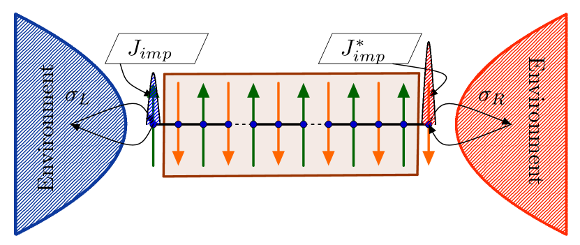
As shown in the Fig.1, the model describes the spin chain interacting with magnetic bath with spin exchange interaction. To understand the application of the model in a broader context, let us recall the well known fact that the low energy effective field theoretic description of the Heisenberg chain is given by Weiss-Zumino-Witten theory perturbed by a marginal operator [60]. In terms of the quadratic current, the low energy theory can be written as
| (6) |
where is the coupling constant for the marginally irrelevant Thirring term and the level in our case. Adding the boundary perturbation described in Eq.(4), the low energy description of Eq.(4) is given by the Hamiltonian [61]
| (7) |
where and are the spin operators of the impurities at the edges of spin chain.
From Eq.(7), it is evident that this model describes the spin part of an interacting system with two non-Hermitian Kondo-like impurities at the edges. Recently, the non-Hermitian Kondo model in a non-interacting Fermi-liquid has been studied as an archetypal model for the Kondo effect in dissipative system[50, 59]. Here we advance the study of quantum spin chains with boundary (Kondo) couplings to include interactions in the bulk part of the system thus fundamentally going beyond previous limits of the problem. At the same time, our results share many common features with the dissipative Kondo model including bound modes and first order like transitions that are fundamentally beyond what is possible in the Hermitian model.
III Summary of the Results
Before describing our solution of the model, let us briefly summarize our main results. The model has three distinct phases characterized by (explicitly written in Eq.(36)) which is related to the bulk and boundary couplings via Eq.(5) as shown in the phase diagram Fig.2. In two of the three phases, the symmetry is unbroken, where as in one of the phases, the symmetry is spontaneously broken.
-
•
Dissipative Kondo effect: For even , when , impurities are screened due to the multiparticle Kondo-like effect. The ground state is a unique singlet state, and no boundary excitations are possible at low energies. All states within this phase possess real energies in the thermodynamic limit, demonstrating unbroken symmetry. If the total number of sites is odd, then there is a spinon in the ground state state which could be oriented in the positive or negative direction thereby the ground state is two fold degenerate with and both the impurities are screened by Kondo clouds at the respective edges. When a global magnetic field is applied by adding a Zeeman term to the Hamiltonian, the local impurity magnetization changes smoothly from and to at where the entire spin chain polarizes.
-
•
Spontaneously broken symmetry: When , the ground state is a singlet where the bulk is a sea of singlets, and the boundary impurities are screened by bound modes formed at the impurity sites. Boundary excitations involve removal of the bound mode at one or both ends. The states containing an odd number of bound modes have complex energies whereas the ones containing an even number of bound modes have real energies. When a global magnetic field is applied by adding a Zeeman term to the Hamiltonian, the local impurity magnetization no longer smoothly changes from to but rather has an abrupt jump at some value of magnetic field . This abrupt jump in magnetic field shows that the bound mode is present in the ground state in this regime.
Moreover, when , the ground state is four-fold degenerate where both impurities are unscreened. Boundary excitations involve screening of the impurities because of the formation of bound modes at the impurity sites. The states containing either zero or two of bound modes have real energies, and those containing a single bound mode have complex energies. States featuring bound modes only at the left edge have corresponding partner states with bound modes only at the right edge, characterized by complex conjugate energies. The states with complex energies always appear in pair demonstrating that the symmetry is spontaneously broken in this phase.
-
•
Effectively free local moment: When , the ground state is four-fold degenerate state where both impurities are unscreened. There are no excitations in this phase which can screen the impurities. In this phase, all states have real energies in the thermodynamic limit, illustrating the unbroken symmetry.
After the brief description of the result, we are now ready to present the Bethe Ansatz and DMRG results obtained for each phase.
IV Bethe Ansatz and DMRG results
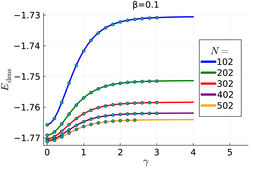
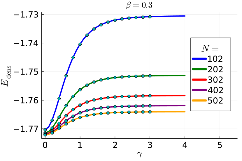
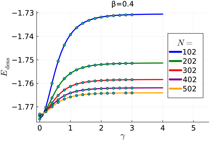
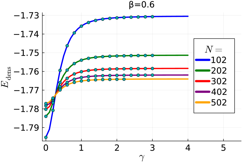
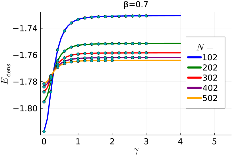
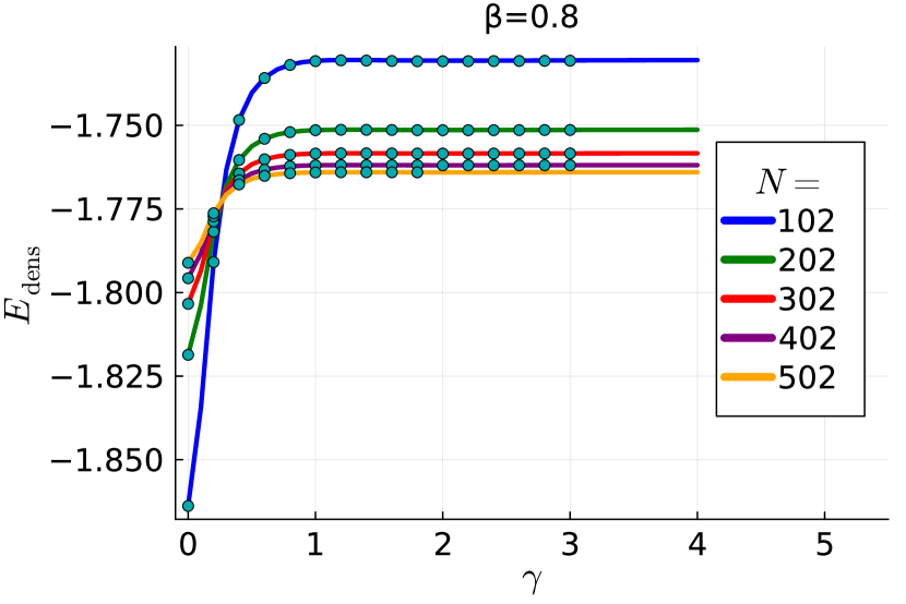
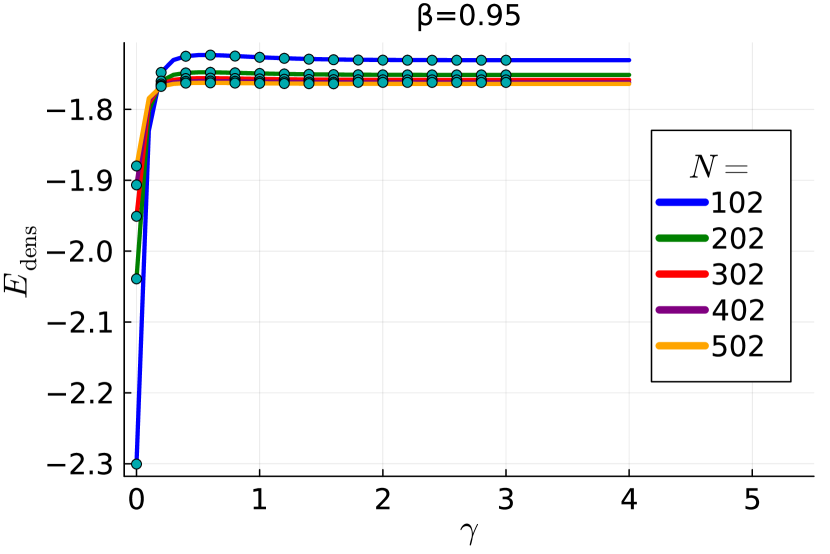
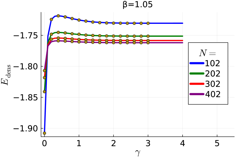
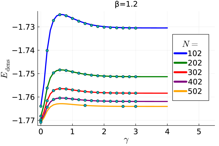
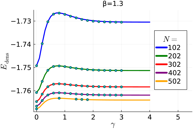
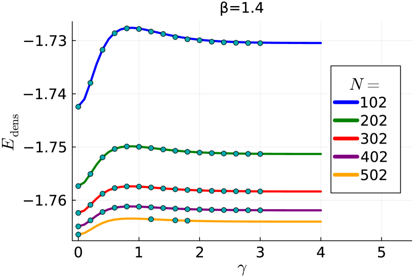
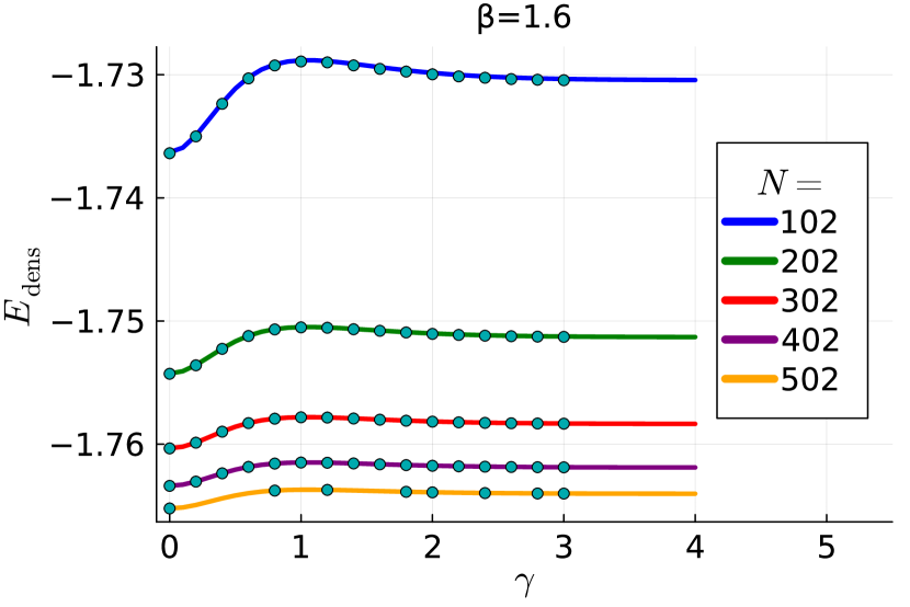
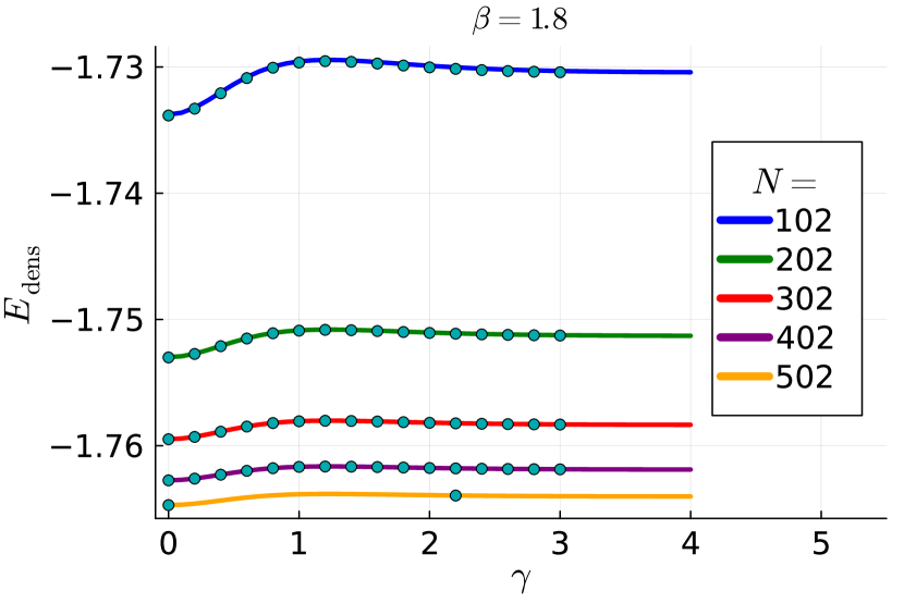
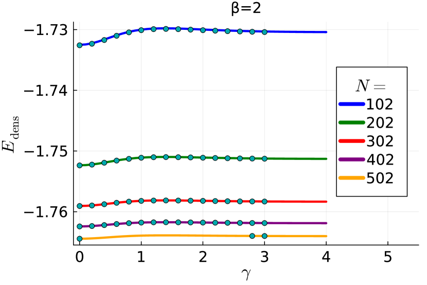
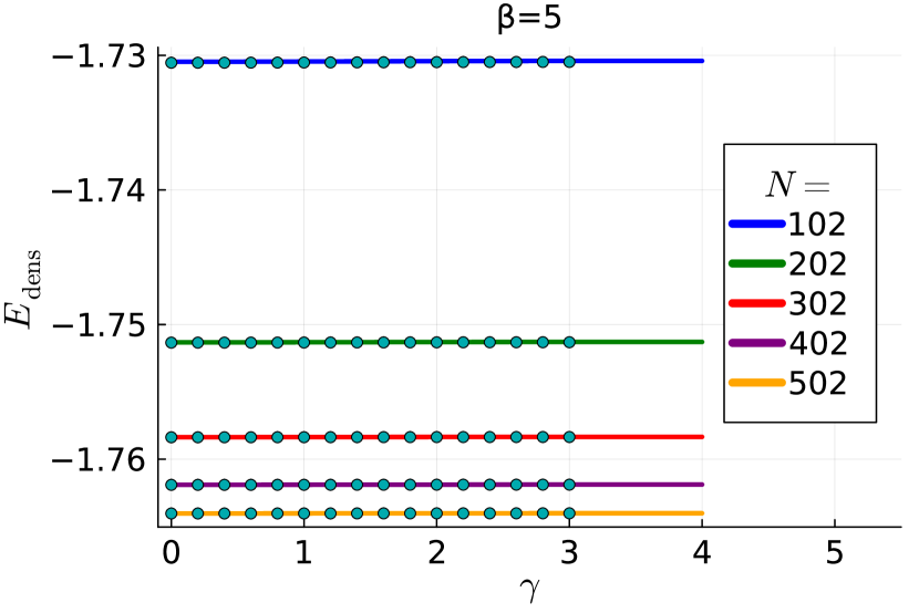
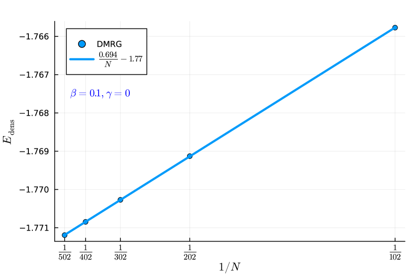
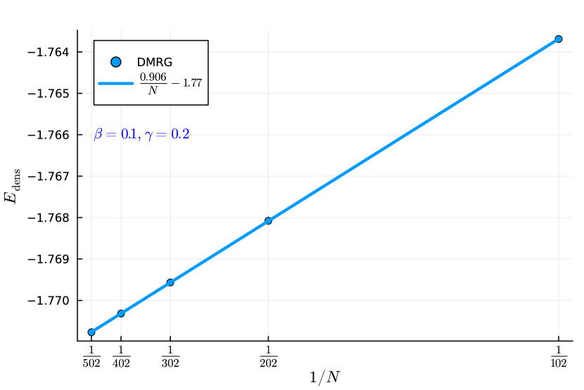
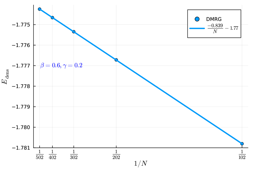
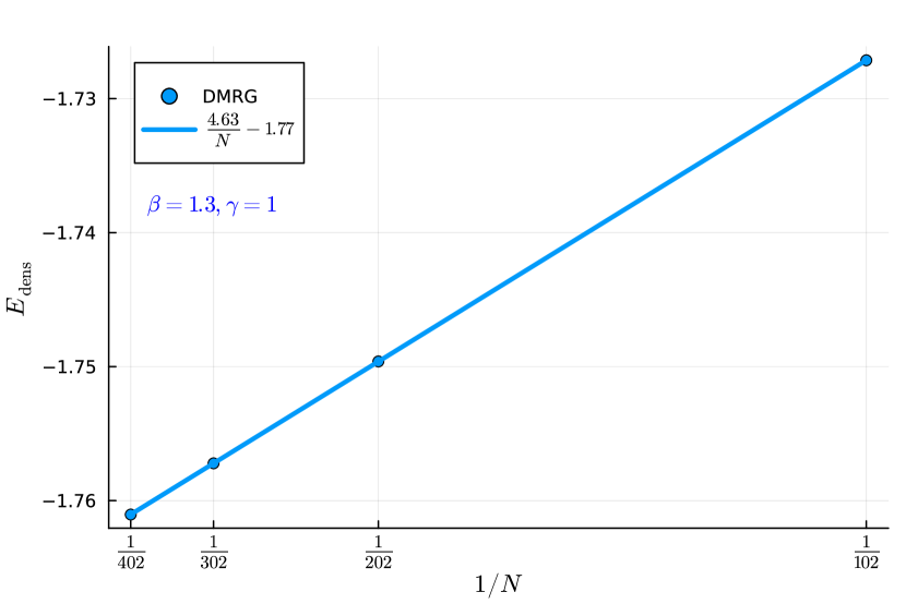
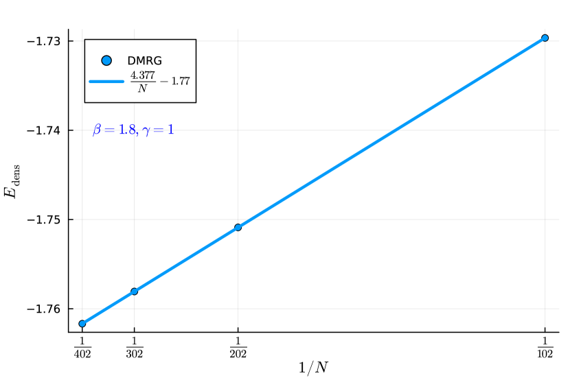
We shall now proceed to discuss the Bethe Ansatz and DMRG results in much detail in this section. We shall describe the structure of the ground state and elementary excitations in all three boundary phases. To make concrete quantitative comparison of the Bethe Ansatz and DMRG results, in the following we work at a fixed truncation error in the discarded singular values at and we obtain the energy density from DMRG with non-Hermitian matrix product operators for various system sizes . As there is always a ground state energy in this model, we fit the ground state energy density to determine the bulk and boundary contributions from the functional form
| (8) |
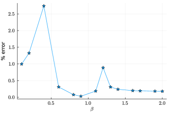
where the slope (as a function of ) is the combined energy density contribution due to the open boundary and the interaction with the impurities. Henceforth, we refer to as the boundary part of energy density and is the energy density of the bulk. From the fit, we extract and for various parameters and compare with the the exact result obtained for from Bethe Ansatz (see Appendix C Fig.17 and Fig.18 for details). In each boundary phase of the model, the exact value of remains the same at , which is the energy density of the Hermitian XXX chain with periodic boundary conditions. On the other hand, depends on each boundary phase and we present a detailed error estimate in the DMRG estimate of relative to its exact value we derive with Bethe ansatz in the following.
IV.1 The dissipative Kondo phase
When the parameter takes the values between 0 and , both impurities are screened by a dissipative multi particle Kondo clouds in the ground state. As we shall see, all eigenstates in this phase have real eigenvalues. Thus, the ground state is defined in the usual sense as the state with lowest energy. The ground state is a multiparticle singlet with real energy given by Eq.(50) which is calculated using both Bethe Ansatz and DMRG (see Appendix B.1 for details). In the Kondo phase in the thermodynamic limit is
| (9) |
where is the logarithmic derivative of the gamma function also called as the digamma function.
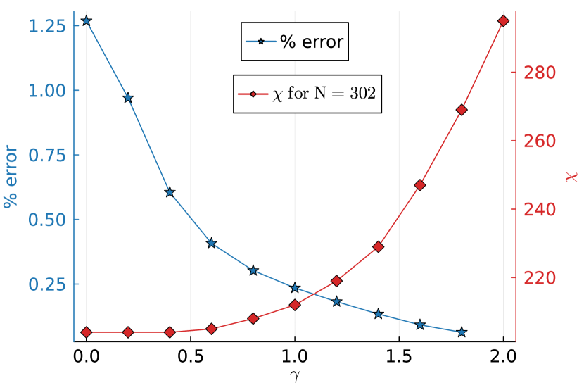
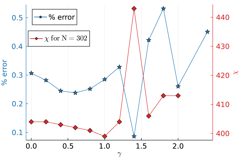
We find that the bulk part of energy density obtained from the DRMG calculation and Bethe Ansatz result in thermodynamic limit has a relative percentage difference of about for any value of and within the Kondo phase. The boundary term suffers larger finite size effects and hence has a larger relative error compared to the bulk part. The relative difference in the values of between the Bethe Ansatz result in Eq. (9) and DMRG for a representative case of and various values of parameter as shown in Fig.3 along with the bond dimension required to attain convergence with the truncation cut off set for sites. We perform 50 sweeps to ensure convergence for every data points. Importantly, as we show in Appendix C.1, the quality of convergence in the boundary energy density is comparable to what we find in the same model in the limit of a Hermitian coupling showing that the DMRG does not suffer any loss of performance despite the non-Hermitian boundary couplings.
All the excited states are constructed by adding an even number of spinons, bulk strings, quartets etc [62] all of which have real energies. Thus, all the excitations in this phase are completely real which shows that symmetry remains unbroken in this phase.
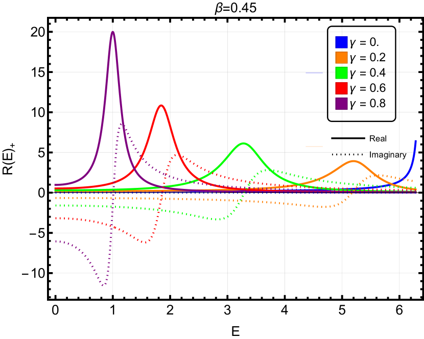
The non-Hermitian Kondo regime is characterized by a dynamically generated complex scale [59]. The real part of this temperature is the characteristic Kondo temperature, the dynamically generated energy scale below which the impurities are screened by the Kondo effect and the imaginary part sets the scale for dynamically balanced loss and gain at the two edges of the chain. The effect of this multiparticle screening can be seen in the enhancement of the local impurity density of states among other physical quantities. The ratio of the impurity and bulk contribution to the density of states is (explicitly computed in Appendix B)
| (10) |
where the positive sign corresponds to left boundary impurity and the negative sign corresponds to the right boundary impurity.
Notice that even though the ground state is real because of the balanced gain and loss at the two boundaries, the physical quantities concerning only one boundary impurity is not real. Hence, the ratio of the density of states of the impurity to that of the bulk is not real for single impurity. This quantity is shown in Fig.4 for various values of and . The shift in the density of states away from the Fermi level may be observed by STM measurements [63].
Defining the Kondo temperature as a characteristic energy scale below which the number of states is exactly half of the total number of states associated with the impurity i.e [44]
| (11) |
where the impurity DOS is given by Eq.(53)
| (12) |
such that the Kondo temperature becomes
| (13) |
where the ve sign is for the impurity at the left end and the ve sign is for the impurity situated at the right end of the chain. Due to the symmetry, the Kondo temperatures corresponding to the left and right impurities are complex conjugates of each other, reflecting the dynamically balanced loss and gain at the two edges of the chain.

We shall now study the model in the presence of a global magnetic field by adding a Zeeman term
| (14) |
to the Hamiltonian. In order to study the impurity physics in the presence of the magnetic field, we shall use DMRG and study the local magnetization at the impurity site
| (15) |
for a spin chain of size bulk sites and 2 impurities (thus a spin chain of total sites) and perform DMRG using the ITensor library [36]. All DMRG calculations are performed with a truncation error cut-off of . Depending on the value of magnetic field and the boundary coupling, the calculation converges after different number of sweeps. Thus, to ensure the convergence for all ranges of parameter, we used 50 sweeps for all calculation.
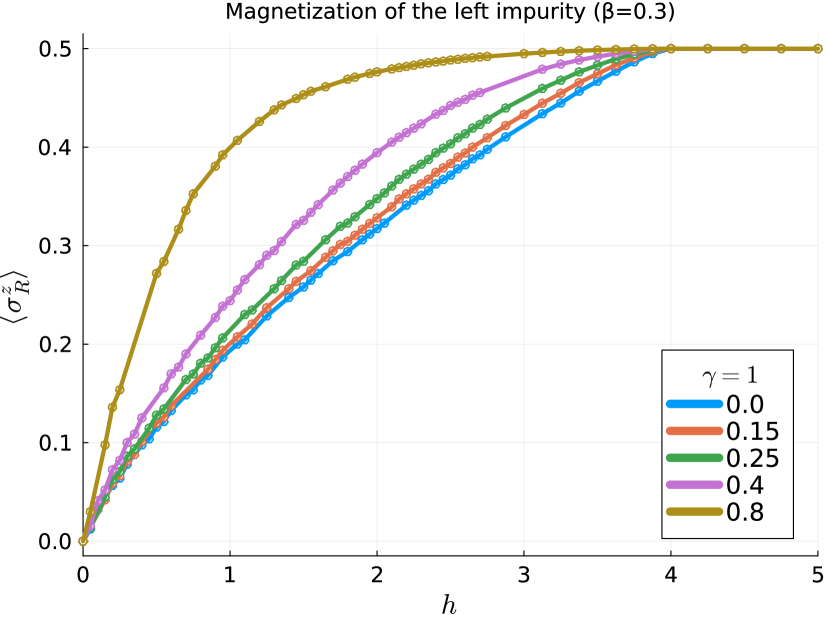
In the Kondo phase, we fix between 0 and 0.5 and vary , and compute the local magnetization of the impurity. The plot of the impurity magnetization in Fig.5 shows that it smoothly crosses over from 0 and to at finite field exactly as in the Hermitian case [44] for all values of . Notice that both left and right impurity magnetization is qualitatively the same as shown in the representative figure below for which resembles the impurity magnetization behavior of the usual Kondo problem [64].
IV.2 Bound mode phases with spontaneously broken symmetry
When , a boundary bound mode appears in the spectrum of the model. The properties of the ground state in this phase depend on when is smaller or larger than . Thus, we further divide the bound mode phase into two regimes: the bound mode phase I when where the bound mode has negative real part of the energy and hence it is contained in the ground state and the bound mode II phase when where the bound mode has positive real part of the energy and thus it is not in the ground state.
IV.2.1 Bound mode phase I
When , both impurities are screened in the ground state by two bound modes formed at their respective edges. These bound modes are described by the two boundary string solutions of the Bethe Ansatz equation
| (16) |
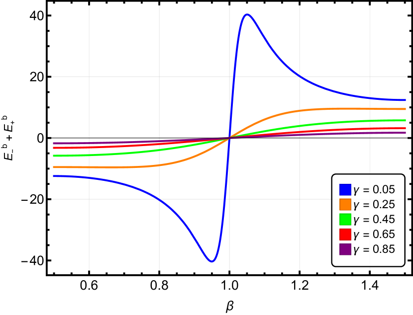
and they have energy
| (17) |
Notice that in the Hermitian case, the boundary string solutions are purely imaginary solutions of the Bethe equation with real energy that describe the boundary excitations [65, 66, 67, 68, 46, 69, 45, 47]. Here, the boundary string solutions are complex and they describe the dissipative boundary excitations in the model as the energy eigenvalues of these solutions are complex. The sum of the energies of two bound modes is real and negative as shown in Fig.6.
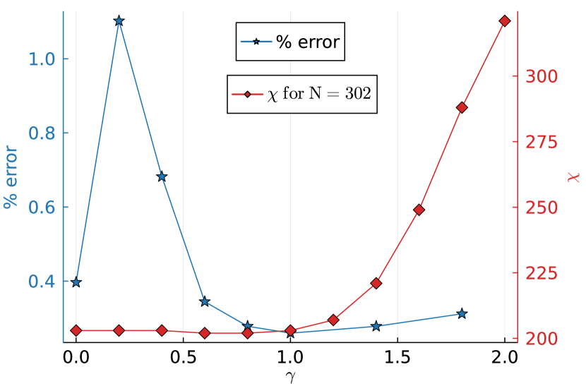
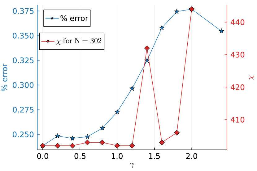
Thus, the ground state contains both boundary strings such that the ground state energy is real as given by Eq.(67). The boundary part of the energy density (i.e. introduced in Eq. (8) and explicitly given by Eq. (8)) is computed from both Bethe Ansatz and DMRG and the relative difference between the two methods is shown in Fig.7 versus for the representative case of . The bond dimension required for the convergence when the truncation cut-off is set at for total number of sites is also shown in Fig.7.
In the Hermitian limit , the energies of the bound mode diverge when . But any non-zero , the real part of the energy of the bound mode vanishes at . Recall that the bulk excitations (spinon) can have energies in the range and in the Hermitian limit, the energy of the bound mode is in the range which shows the clear demarcation between the bulk and boundary excitations. However, as shown in Fig.6, when , the boundary excitation can also have any energy , thereby making the demarcation of the bulk and boundary excitation flimsy. This behavior was also seen in the case of complex boundary field studied in [46]. For any fixed , , when . Thus, for large , the bound mode ceases to exist and hence, the difference between the bound mode and unscreened phases becomes negligible.
Since the sum of the energies of the two boundary strings are negative when , the ground state contains these bound modes. The ratio of the density of states contribution of impurity to bulk becomes
| (18) |
where is given by Eq.(10). In this regime real part of the is negative and hence the only positive contribution to the screening of the impurity comes from the two bound modes each located at their respective edges of the spin chain.
We can construct excited state solutions by removing one boundary string and adding a zero-energy spinon or by removing both boundary string solutions. Thus, there are four distinct kinds of elementary states that can be sorted into four distinct sets shown in the schematic Fig.8 described below:
-
1.
A unique state where each impurity is screened by a bound mode formed at the respective edge, which possesses real energy.
-
2.
A four-fold degenerate state with the left impurity screened by a bound mode, the right impurity unscreened, and a spinon propagating in the bulk. This state has complex energy.
-
3.
A four-fold degenerate state with the right impurity screened by a bound mode, the left impurity unscreened, and a spinon propagating in the bulk. This state also has complex energy, with its energy being the complex conjugate of the state described in 2.
-
4.
A four-fold degenerate state with both impurities unscreened, which possesses real energy.
To each of these states, we can add an even number of spinons, bulk strings, quartets and higher order boundary strings to form four distinct sets of excited states which are characterized by the number of the bound modes at two edges. All the states in the first set have two bound modes whereas the ones in fourth set have no bound modes. All the states in both the first and fourth sets have real energies and an even number of spinons. The states in the second set have only one bound mode at the left end and all the states have complex energies. Moreover, all the states in the third set have only one bound mode at the right end and all the states have complex energies that are complex conjugate to the energies of the states in second set. The total number of spinons in each state in second and third set is odd. The presence of the states in pair with complex conjugate energy is the signature of the spontaneously broken symmetry. It is important to remember that only for smaller value of where the real part of the boundary string given by Eq.(17) is sufficiently bigger than , the distinction between the sets of eigenstates becomes apparent but when , the real part of the bound mode energy approaches as shown in Fig.6 and hence experimentally detecting the effect of bound mode becomes difficult. Thus, for large , the demarcation between the different sets of excited states becomes rickety. In the Hermitian limit, since the boundary bound mode always have energy greater than the maximum energy of the spinon , the four sets form a well defined towers of excited states [44, 70].
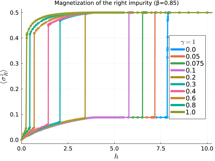
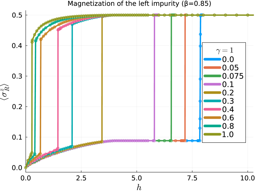
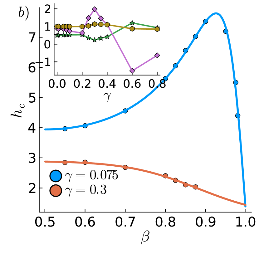
We shall now study the model in the presence of global magnetic field by adding Zeeman term given by Eq.(14). In the bound mode phase I, by taking and varying , we compute the local impurity magnetization. Because of the presence of the boundary bound modes in the ground state, the local impurity magnetization abruptly jumps in in the bound mode phase just like in the Hermitian case [44]. Both left and right impurity magnetizations are qualitatively the same as shown in the representative figure Fig.9 for model parameter and various values of .
It is well known that the periodic Heisenberg chain is fully polarized when . Here, we see an interesting trend that if the critical value of the field , then the local impurity magnetization smoothly increases from at and then attains a finite value at up until which there are bulk degrees of freedom to polarize, then the magnetization becomes constant until where it suddenly jumps to as shown in Fig.9. This sudden jump is because there are just two unpolarized bound modes left in the model above and when the energies of these modes in the presence of the magnetic field are equal to the applied field, the modes flip thereby unscreening both impurities. However, if , then the magnetization increases smoothly till , and makes a finite jump due to the contribution from the boundary string solution. This time, however, there are sill some bulk degrees of freedom to excite, thus the magnetization does not reach 0.5 after the jump but reaches some finite values. When is increased above , the impurity magnetization further smoothly increases to at at this point the impurity is completely unscreened.
For a fixed value of , if is varied or if is fixed and is varied, then the value of the critical field at which the impurity magnetization jumps can be fitted to a function of the form
| (19) |
where the parameters for various values of in the bound mode phase I are shown in Fig. 10 a). Likewise, we fit the critical field for fixed when is varied in Fig.10 b). Unlike in the Hermitian case, the relation between the critical field and the complex eigenvalue of the bound mode seems to be more complicated in this case. For example, the vertical jump i.e. the magnetization difference at the critical value of field for fixed as a function of parameter is non-trivial as shown in Fig.10 c).
IV.2.2 Bound mode phase II
When , the sum of the energies of the two bound modes is positive as shown in Fig.6. Hence the ground state is the state that does not contain any boundary strings. The ground state is thus constructed by adding all the real roots of Bethe Ansatz equations whose energy is explicitly given in Eq. (88). Just as in the Kondo and bound mode phases, we write the energy as the bulk and boundary part given by Eq.(8). The boundary part of the energy density is now given by
| (20) |
The boundary part of energy density extracted from DMRG by fitting data for various system size ( and ) is plotted in Fig.11 for representative parameter as a function of the model parameter .
In the Hermitian limit where and , the sign of the impurity coupling changes from antiferromagnetic to ferromagnetic. However, when , the sign (of the real part) of the coupling varies based on the values of both and . This variation in sign is not indicative of a phase transition. The phase transition point is determined solely by the parameter , regardless of where the coupling changes sign.
The same four distinct states listed in Bound mode phase I described in Sec.IV.2.1 exist in this phase. But the sum of the energies of the two bound modes at the edges is positive as shown in Fig.6. Thus energy of the state with no bound modes on both edges is smaller than the energy of the state with contain both bound modes. Thus, both impurities are unscreened in the ground state but there are excited state where one or both boundary impurities are screened. Just as in Bound mode regime I, there are four distinct sets of excited states
-
1.
The set of excited states that contain states with no bound modes at both ends have all the states with real energies. Both impurities are unscreened in each state in this set and each state have an even number of spinons.
-
2.
The set of excited states where all states have left impurity screened by bound mode but right impurity is unscreened. There are odd number of spinons in each state in this set and all states have complex energies.
-
3.
The set of excited states where all states have right impurity screened by bound mode but left impurity is unscreened. There are odd number of spinons in in each state in this set and all states have complex energies which are complex conjugates of the energies of states described in 2.
-
4.
The set of excited states that contain states with two bound modes at each end have all the states with real energies. Both impurities are screened in each state in this set and each state have an even number of spinons.
IV.3 Unscreened local moment phase
When , the impurities can not be screened in any eigenstates in this phase. Both impurities are unscreened in the ground state and hence the ground state is four-fold degenerate in the thermodynamic limit with real energy given by Eq.(88). The boundary part of the energy density is given by Eq.(20). We extract from DMRG by fitting the energy for various system size to Eq.(8) and plot the relative difference between the result obtained from Bethe Ansatz in thermodynamic limit to the result obtained from DMRG in Fig.12 for as a function of .
All the excited states can be constructed by adding an even number of spinons, bulk strings, quartets etc. all of which have real energies. Thus, all the excited states in this phase have real energies and an even number of spinons.
V Conclusion and Outlook
We considered the integrable Heisenberg spin chain with complex boundary impurity and studied it using a combination of Bethe Ansatz and DMRG techniques. We showed that , a complicated function of the bulk coupling , the absolute value of the boundary coupling and the real part of the boundary coupling given in Eq.(36), governs the phase transitions. There are four distinct phases in the model. When , the model is in the Kondo phase where both impurities are screened by multiparticle Kondo cloud characterized by a peak in local density of states. When , the model is in the bound mode phase I where both impurities are screened by bound modes formed at each impurity site in the ground state. There are, however, excited states where impurities can be unscreened by removing the bound mode solution. When increases to the range , the model is in the bound mode II phase, where the impurities are unscreened in the ground state, but they can be screened by bound modes formed at the impurity sites in the excited states. Finally, when the parameter , the impurities cannot be screened in any eigenstates, and therefore the model is in the unscreened phase.
In the Kondo and unscreened phases, all the eigenstates have real energies, which shows that the symmetry is unbroken in these phases. However, in the two bound mode phases, there are states with real energies and complex energies. For each state with complex energy, there is a state with complex conjugate energy which shows that the symmetry is spontaneously broken in these phases.
As one moves across the phase transition point between the Kondo and bound mode phase I, the ground state undergoes a change where the two multiparticle Kondo clouds which screen the two impurities in the Kondo phase turn into two bound modes which screen the respective impurities. The eigenstates also undergo drastic changes reorganizing the entire Hilbert space as states with all real energies divide into four distinct sets of excited states: two with real energies and two with complex energies.
We showed that the ITensor library’s DMRG algorithm works well for an fully interacting many-body non-Hermitian model by comparing the ground state energy with exact Bethe Ansatz result and then used DMRG to compute local impurity magnetization. A through study of benchmarking the non-Hermitian DMRG will be a subject of upcoming publication.
VI Acknowledgement
We thank Miles Stoudenmire for helpful suggestions and discussions. J.H.P. is partially supported by the Army Research Office Grant No. W911NF-23-1-0144 and NSF Career Grant No. DMR- 1941569.
References
- Lindblad [1976] G. Lindblad, On the generators of quantum dynamical semigroups, Communications in Mathematical Physics 48, 119 (1976).
- Gorini et al. [1976] V. Gorini, A. Kossakowski, and E. C. G. Sudarshan, Completely positive dynamical semigroups of n-level systems, Journal of Mathematical Physics 17, 821 (1976).
- Manzano [2020] D. Manzano, A short introduction to the lindblad master equation, Aip Advances 10 (2020).
- Dattagupta and Puri [2004] S. Dattagupta and S. Puri, Dissipative phenomena in condensed matter: some applications, Vol. 71 (Springer Science & Business Media, 2004).
- Weiss [2012] U. Weiss, Quantum dissipative systems (World Scientific, 2012).
- Koch and Budich [2022] F. Koch and J. C. Budich, Quantum non-hermitian topological sensors, Physical Review Research 4, 013113 (2022).
- Cao et al. [2020] W. Cao, X. Lu, X. Meng, J. Sun, H. Shen, and Y. Xiao, Reservoir-mediated quantum correlations in non-hermitian optical system, Physical Review Letters 124, 030401 (2020).
- Wouters and Carusotto [2007] M. Wouters and I. Carusotto, Excitations in a nonequilibrium bose-einstein condensate of exciton polaritons, Physical review letters 99, 140402 (2007).
- Fitzpatrick et al. [2017] M. Fitzpatrick, N. M. Sundaresan, A. C. Li, J. Koch, and A. A. Houck, Observation of a dissipative phase transition in a one-dimensional circuit qed lattice, Physical Review X 7, 011016 (2017).
- Botzung et al. [2021] T. Botzung, S. Diehl, and M. Müller, Engineered dissipation induced entanglement transition in quantum spin chains: From logarithmic growth to area law, Physical Review B 104, 184422 (2021).
- Alberton et al. [2021] O. Alberton, M. Buchhold, and S. Diehl, Entanglement transition in a monitored free-fermion chain: From extended criticality to area law, Physical Review Letters 126, 170602 (2021).
- Yu and Zhang [2008] H. Yu and J. Zhang, Understanding hawking radiation in the framework of open quantum systems, Physical Review D 77, 024031 (2008).
- Kaplanek and Burgess [2020] G. Kaplanek and C. Burgess, Hot cosmic qubits: late-time de sitter evolution and critical slowing down, Journal of High Energy Physics 2020, 1 (2020).
- Chakraborty et al. [2022] A. Chakraborty, H. Camblong, and C. Ordóñez, Thermal effect in a causal diamond: Open quantum systems approach, Physical Review D 106, 045027 (2022).
- Rotter [2009] I. Rotter, A non-hermitian hamilton operator and the physics of open quantum systems, Journal of Physics A: Mathematical and Theoretical 42, 153001 (2009).
- Müller and Rotter [2009] M. Müller and I. Rotter, Phase lapses in open quantum systems and the non-hermitian hamilton operator, Physical Review A 80, 042705 (2009).
- Savin et al. [2003] D. V. Savin, V. V. Sokolov, and H.-J. Sommers, Is the concept of the non-hermitian effective hamiltonian relevant in the case of potential scattering?, Physical Review E 67, 026215 (2003).
- Ashida et al. [2020] Y. Ashida, Z. Gong, and M. Ueda, Non-hermitian physics, Advances in Physics 69, 249 (2020).
- Breuer and Petruccione [2002] H.-P. Breuer and F. Petruccione, The theory of open quantum systems (Oxford University Press, USA, 2002).
- Prosen [2008] T. Prosen, Third quantization: a general method to solve master equations for quadratic open fermi systems, New Journal of Physics 10, 043026 (2008).
- Medvedyeva et al. [2016] M. V. Medvedyeva, F. H. L. Essler, and T. c. v. Prosen, Exact bethe ansatz spectrum of a tight-binding chain with dephasing noise, Phys. Rev. Lett. 117, 137202 (2016).
- Alba [2023] V. Alba, Free fermions with dephasing and boundary driving: Bethe ansatz results, arXiv preprint arXiv:2309.12978 (2023).
- Castaldi et al. [2013] G. Castaldi, S. Savoia, V. Galdi, A. Alu, and N. Engheta, P t metamaterials via complex-coordinate transformation optics, Physical review letters 110, 173901 (2013).
- Yin and Zhang [2013] X. Yin and X. Zhang, Unidirectional light propagation at exceptional points, Nature materials 12, 175 (2013).
- Zyablovsky et al. [2014] A. A. Zyablovsky, A. P. Vinogradov, A. A. Pukhov, A. V. Dorofeenko, and A. A. Lisyansky, Pt-symmetry in optics, Physics-Uspekhi 57, 1063 (2014).
- Klauck et al. [2019] F. Klauck, L. Teuber, M. Ornigotti, M. Heinrich, S. Scheel, and A. Szameit, Observation of pt-symmetric quantum interference, Nature Photonics 13, 883 (2019).
- Kawabata et al. [2018] K. Kawabata, Y. Ashida, H. Katsura, and M. Ueda, Parity-time-symmetric topological superconductor, Physical Review B 98, 085116 (2018).
- Kornich and Trauzettel [2022] V. Kornich and B. Trauzettel, Signature of p t-symmetric non-hermitian superconductivity in angle-resolved photoelectron fluctuation spectroscopy, Physical Review Research 4, L022018 (2022).
- Bagarello et al. [2015] F. Bagarello, M. Lattuca, R. Passante, L. Rizzuto, and S. Spagnolo, Non-hermitian hamiltonian for a modulated jaynes-cummings model with pt symmetry, Physical Review A 91, 042134 (2015).
- Zhao and Lu [2017] Y. Zhao and Y. Lu, P t-symmetric real dirac fermions and semimetals, Physical review letters 118, 056401 (2017).
- Turker et al. [2018] Z. Turker, S. Tombuloglu, and C. Yuce, Pt symmetric floquet topological phase in ssh model, Physics Letters A 382, 2013 (2018).
- Bender and Boettcher [1998] C. M. Bender and S. Boettcher, Real spectra in non-hermitian hamiltonians having p t symmetry, Physical review letters 80, 5243 (1998).
- Wigner [1960] E. P. Wigner, Phenomenological distinction between unitary and antiunitary symmetry operators, Journal of Mathematical Physics 1, 414 (1960).
-
Note [1]
Consider the Schrodinger equation
Acting with a generic anti-linear operator , we arrive at:(21)
In Eq.(22), we find that when the Hamiltonian obeys the antilinear symmetry condition , two distinct scenarios emerge, as originally pointed out by Wigner: a) If the eigenfunctions satisfy , then the corresponding eigenvalues are real.(22)
b)Alternatively, when the eigenfunctions exhibit the property , the energies appear in conjugate pairs, and the conjugate eigenfunctions take the form and . - Mostafazadeh [2003] A. Mostafazadeh, Exact pt-symmetry is equivalent to hermiticity, Journal of Physics A: Mathematical and General 36, 7081 (2003).
- Fishman et al. [2022] M. Fishman, S. White, and E. Stoudenmire, The itensor software library for tensor network calculations, SciPost Physics Codebases , 004 (2022).
- Bender et al. [2004] C. M. Bender, D. C. Brody, and H. F. Jones, Extension of pt-symmetric quantum mechanics to quantum field theory with cubic interaction, Physical Review D 70, 025001 (2004).
- Bender and Tan [2006] C. M. Bender and B. Tan, Calculation of the hidden symmetry operator for a-symmetric square well, Journal of Physics A: Mathematical and General 39, 1945 (2006).
- Bethe [1931] H. A. Bethe, Zur Theorie der Metalle. i. Eigenwerte und Eigenfunktionen der linearen Atomkette, Zeit. für Physik 71, 205 (1931).
- Alcaraz et al. [1987] F. C. Alcaraz, M. N. Barber, M. T. Batchelor, R. Baxter, and G. Quispel, Surface exponents of the quantum xxz, ashkin-teller and potts models, Journal of Physics A: mathematical and general 20, 6397 (1987).
- Sklyanin [1988] E. K. Sklyanin, Boundary conditions for integrable quantum systems, Journal of Physics A: Mathematical and General 21, 2375 (1988).
- Wang et al. [2015] Y. Wang, W.-L. Yang, J. Cao, and K. Shi, Off-diagonal Bethe ansatz for exactly solvable models (Springer, 2015).
- Frahm et al. [2010] H. Frahm, J. H. Grelik, A. Seel, and T. Wirth, Functional bethe ansatz methods for the open xxx chain, Journal of Physics A: Mathematical and Theoretical 44, 015001 (2010).
- Kattel et al. [2024a] P. Kattel, P. R. Pasnoori, J. H. Pixley, P. Azaria, and N. Andrei, Kondo effect in the isotropic heisenberg spin chain, Phys. Rev. B 109, 174416 (2024a).
- Wang [1997] Y. Wang, Exact solution of the open heisenberg chain with two impurities, Physical Review B 56, 14045 (1997).
- Kattel et al. [2023] P. Kattel, P. R. Pasnoori, and N. Andrei, Exact solution of a non-hermitian-symmetric spin chain, Journal of Physics A: Mathematical and Theoretical 56, 325001 (2023).
- Frahm and Zvyagin [1997] H. Frahm and A. A. Zvyagin, The open spin chain with impurity: an exact solution, Journal of Physics: Condensed Matter 9, 9939 (1997).
- Kattel et al. [2024b] P. Kattel, Y. Tang, J. H. Pixley, and N. Andrei, The kondo effect in the quantum xx spin chain, Journal of Physics A: Mathematical and Theoretical (2024b).
- Ren et al. [2022] Z. Ren, D. Liu, E. Zhao, C. He, K. K. Pak, J. Li, and G.-B. Jo, Chiral control of quantum states in non-hermitian spin–orbit-coupled fermions, Nature Physics 18, 385 (2022).
- Nakagawa et al. [2018] M. Nakagawa, N. Kawakami, and M. Ueda, Non-hermitian kondo effect in ultracold alkaline-earth atoms, Physical review letters 121, 203001 (2018).
- Cao et al. [2023] M.-M. Cao, K. Li, W.-D. Zhao, W.-X. Guo, B.-X. Qi, X.-Y. Chang, Z.-C. Zhou, Y. Xu, and L.-M. Duan, Probing complex-energy topology via non-hermitian absorption spectroscopy in a trapped ion simulator, Physical Review Letters 130, 163001 (2023).
- Lu et al. [2024] P. Lu, T. Liu, Y. Liu, X. Rao, Q. Lao, H. Wu, F. Zhu, and L. Luo, Realizing quantum speed limit in open system with a-symmetric trapped-ion qubit, New Journal of Physics 26, 013043 (2024).
- Dogra et al. [2021] S. Dogra, A. A. Melnikov, and G. S. Paraoanu, Quantum simulation of parity–time symmetry breaking with a superconducting quantum processor, Communications Physics 4, 26 (2021).
- Chen et al. [2021] W. Chen, M. Abbasi, Y. N. Joglekar, and K. W. Murch, Quantum jumps in the non-hermitian dynamics of a superconducting qubit, Physical Review Letters 127, 140504 (2021).
- Zhang et al. [2020] R. Zhang, Y. Cheng, P. Zhang, and H. Zhai, Controlling the interaction of ultracold alkaline-earth atoms, Nature Reviews Physics 2, 213 (2020).
- Gorshkov et al. [2010] A. V. Gorshkov, M. Hermele, V. Gurarie, C. Xu, P. S. Julienne, J. Ye, P. Zoller, E. Demler, M. D. Lukin, and A. Rey, Two-orbital su (n) magnetism with ultracold alkaline-earth atoms, Nature physics 6, 289 (2010).
- Jepsen et al. [2020] P. N. Jepsen, J. Amato-Grill, I. Dimitrova, W. W. Ho, E. Demler, and W. Ketterle, Spin transport in a tunable heisenberg model realized with ultracold atoms, Nature 588, 403 (2020).
- Schwager et al. [2013] H. Schwager, J. I. Cirac, and G. Giedke, Dissipative spin chains: Implementation with cold atoms and steady-state properties, Physical Review A 87, 022110 (2013).
- Kattel et al. [2024c] P. Kattel, A. Zhakenov, P. R. Pasnoori, P. Azaria, and N. Andrei, Dissipation driven phase transition in the non-hermitian kondo model, arXiv preprint arXiv:2402.09510 (2024c).
- Affleck [1986] I. Affleck, Exact critical exponents for quantum spin chains, non-linear -models at = and the quantum hall effect, Nuclear Physics B 265, 409 (1986).
- Laflorencie et al. [2008] N. Laflorencie, E. S. Sørensen, and I. Affleck, The kondo effect in spin chains, Journal of Statistical Mechanics: Theory and Experiment 2008, P02007 (2008).
- Destri and Lowenstein [1982] C. Destri and J. Lowenstein, Analysis of the bethe-ansatz equations of the chiral-invariant gross-neveu model, Nuclear Physics B 205, 369 (1982).
- Avraham [2024] N. Avraham, private communication (2024).
- Andrei et al. [1983] N. Andrei, K. Furuya, and J. Lowenstein, Solution of the kondo problem, Reviews of modern physics 55, 331 (1983).
- Kapustin and Skorik [1996] A. Kapustin and S. Skorik, Surface excitations and surface energy of the antiferromagnetic xxz chain by the bethe ansatz approach, Journal of Physics A: Mathematical and General 29, 1629 (1996).
- Pasnoori et al. [2020] P. R. Pasnoori, C. Rylands, and N. Andrei, Kondo impurity at the edge of a superconducting wire, Physical Review Research 2, 013006 (2020).
- Pasnoori et al. [2021] P. R. Pasnoori, N. Andrei, and P. Azaria, Boundary-induced topological and mid-gap states in charge conserving one-dimensional superconductors: Fractionalization transition, Physical Review B 104, 134519 (2021).
- Pasnoori et al. [2022] P. R. Pasnoori, N. Andrei, C. Rylands, and P. Azaria, Rise and fall of yu-shiba-rusinov bound states in charge-conserving s-wave one-dimensional superconductors, Physical Review B 105, 174517 (2022).
- Rylands [2020] C. Rylands, Exact boundary modes in an interacting quantum wire, Physical Review B 101, 085133 (2020).
- Pasnoori et al. [2023] P. R. Pasnoori, J. Lee, J. H. Pixley, N. Andrei, and P. Azaria, Boundary quantum phase transitions in the spin- heisenberg chain with boundary magnetic fields, Phys. Rev. B 107, 224412 (2023).
- Note [2] The energy density becomes independent of the system size for some values of for approximately from 0.35 to 1.17. However, since the energy function is written in terms of digamma functions which are difficult to invert, the analytic expression for the relation between and where the energy density becomes independent of system size is difficult to obtain.
- Note [3] In the Hermitian limit , notice that the expression in Equation (91) exhibits superfluous divergence due to blowing up for . However, there is also a divergent factor in in the digamma functions that cancels out the divergences in the energy of the boundary string. Thus, one can explicitly write as shown in Eq.(91) which is divergence free.
Appendix A Integrability of the Hamiltonian
The rational 6-vertex matrix
| (23) |
where is the identity matrix and is the permutation operator , acts non trivially on the product space such that in ), it satisfies the a non-linear matrix equation
| (24) |
called quantum Yang-Baxter equation (qYBE). We introduce two transfer matrices and
| (25) | ||||
| (26) |
Here each matrix with the spectral parameter is a linear operator acting on the product space where is the local Hilbert space of either the bulk spin (with index 1 through ) or two boundary impurity spins (with index L and R) and is called auxiliary space. The spectral parameter is shifted by and its complex conjugate for the right and left impurities, respectively. The trace of the product of two transfer matrices over the auxiliary space is defined as the double row transfer matrix
| (27) |
It follows from the qYBE Eq.(24) that the transfer matrix is a one-parameter family of commuting operator i.e.
| (28) |
such that it can act as a generator of infinite number of commuting operators which can be diagonalized simultaneously. One of such operators is the Hamiltonian Eq.(4) which is obtained from the transfer matrix as
| (29) |
upon identifying the complex boundary coupling constant as
| (30) |
Each eigenvalues of the transfer matrix Eq.(27) is given by the Baxter’s T-Q relation
| (31) |
where the -function is given by
| (32) |
Regularity of the equation gives the BAEs
| (33) |
Changing the variable and introducing where , we rewrite the above equation as
| (34) |
In terms of the bulk coupling and boundary coupling , the parameters and can be written as
| (36) |
and
| (37) |
In the logarithmic form, the Bethe equations Eq.(34) becomes
| (38) |
Quantum numbers occupy a symmetric interval around the origin. Moreover, thanks to the presence of symmetry in the Hamiltonian, the rapidities in the ground state are real. This, to analyze Eq.(38) in thermodynamics limit, we define the density of Bethe roots as
| (39) |
Such that we convert the sums over in Eq.(35) and Eq.(38) into integral over as
| (40) |
and
| (41) |
We extract the density of roots in the ground state by subtracting Eq.(41) written for from the same equation written for and expanding in the difference . This gives
| (42) |
Since, we are interested in thermodynamics limit , the higher order terms are negligible.
Here,
| (43) | ||||
| (44) | ||||
| (45) |
We will now solve the Bethe equation in various phases which are determined by values of and . It is well known that the solution depends on whether the total number of particles is even or odd. We will focus on the case of an even number of particles. The case for an odd number can be easily generalized as shown in detail in Hermitian case in [44].
Appendix B Solution of Bethe Ansatz equations Eq. (34)
We will now solve the Bethe Ansatz equations when both and are nonzero. In this case the model is non-Hermitian but symmetric as mentioned earlier.
B.1 Kondo phase and
The density of the solutions of Bethe equations can be obtained from an integral equation
| (46) |
where the delta function is added at the origin because the eigenvector corresponding to vanishes.
The solution of Eq.(46) is immediate in Fourier space
| (47) |
such that the total number of Bethe roots is
| (48) |
and hence the total spin in the ground state is
| (49) |
which shows that the impurity is screened by multiparticle Kondo cloud in the ground state.
Using Eq.(35), the energy of this state is
| (50) |
We energy density
| (51) |
for various values of and in the Kondo phase below using the result from both Bethe Ansatz and DMRG are shown in Fig.13. Notice that since the system has a boundary and impurity, the scattering phase shift from the boundary contributes to the energy and hence the energy density is not independent of the system size.

It is important to note that the ground state has real energy in this phase. Also notice that Kondo phase lacks boundary excitations entirely. Moreover, any other excitations in this phase can be constructed by adding an even number of spinons, bulk strings, and quartets, all of which possess real energies. Consequently, all states in the Kondo phase have real energies. Thus, the symmetry is unbroken in this phase.
B.1.1 Spinon density of states
From Eq.(47), we compute the density of state contribution due to the bulk
| (52) |
where we used the spinon energy to write . The impurity part in the Kondo phase gives
| (53) |
Let us now consider the ratio
| (54) |
We compute the Kondo temperature as the energy scale at which the integrated density of state is half of the total number of state
| (55) |
We obtain, the complex Kondo temperature for the left impurity
| (56) |
where the negative sign is for the left impurity and the positive sign is for right impurity and is the maximum energy of spinon.
Notice that even though the ground state energy is real, the spectral weight and the dynamically generated Kondo scale () are complex for each impurity.
B.2 Bound Mode Phase I () and
There are two unique complex solutions in this phase. The first one is
The real part of the energies of both solutions and is negative in the region . Thus, we need to add both of these solutions to construct the ground-state solution. Adding both of these solutions, the integral equation for the root density becomes
| (61) |
The solution of above equation in the Fourier space is
| (62) |
Thus the total number of Bethe roots including the two complex roots and is
| (63) |
Hence, the spin in the ground state is
| (64) |
Both impurities are screened in the ground state by two dissipative bound modes formed at the sites of the two impurities.
The energy of this state is
| (65) |
where is the energy of all real roots which upon using Eq.(35) evaluates to
| (66) |
The ground state energy obtain from Bethe Ansatz given in Eq.(65) and the corresponding result obtained from DMRG is shown in Fig.14 for various parameters in the bound mode phase I.
Notice that
| (67) |
where given by Eq.(50). Notice that for some values of , the energy density becomes independent of system size. For example for at , the energy density becomes independent of the system size 222The energy density becomes independent of the system size for some values of for approximately from 0.35 to 1.17. However, since the energy function is written in terms of digamma functions which are difficult to invert, the analytic expression for the relation between and where the energy density becomes independent of system size is difficult to obtain. which happens because the energy contribution from the impurity independent free boundary exactly cancels the impurity contribution from the two impurities.
There are unique boundary excitations in this phase. We could remove the boundary string solution and add a hole to construct a state whose solution density is given by an integral equation
| (68) |
The solution in the Fourier space reads
| (69) |
The total number of roots including one complex root is
| (70) |
Thus, the spin of this state is
| (71) |
The energy of this state is
| (72) |
This state has unscreened impurity at right edge and one propagating spinon. Because of the SU(2) symmetry, the state is three fold degenerate where the two free spins make triplet pairing. There also exist a state where the unscreened impurity and the hole form singlet pairing. Such a state is constructed by adding both boundary strings and , a hole with rapidity , and the higher order boundary string
| (73) |
The root desnity of the resultant equation is
| (74) |
The total number of roots include three complex roots is
| (75) |
such that the spin of this state is
| (76) |
The energy of this state is
| (77) |
Thus the fundamental boundary excitation involves removal of the bound model screening the impurity and introduction of a hole such that the two free spins form degenerate states. These states, that have screened left impurity and unsceened impurity, have complex energy as is complex.
One can also remove the solution and add a hole or add and a hole to construct the four-fold degenerate state where the left impurity is unscreened and right impurity is screened. The energy of the resultant four states is
| (78) |
The energy of these four-fold degenerate state is complex as is complex.
We can also construct a state described by all real roots which have solution density
| (79) |
The total number of roots is
| (80) |
The spin of this state is
| (81) |
This state contains two unscreened impurities that form triplet pairing. Because of symmetry, this state is three-fold degenerate and which has energy
| (82) |
Because , these state have real energies.
By adding the boundary strings solutions and the higher order string solution , we obtain Bethe equation
| (83) |
such that the solution density becomes
| (84) |
The total number of Bethe roots including the two complex roots is
| (85) |
Thus, the total spin is
| (86) |
Using Eq.(35), we obtain the energy of this state
| (87) |
Thus, this state contains two free impurity spins that forms singlet pairing.
B.3 Bound Mode Phase II and
The two complex solutions and are still valid solutions in this regime, but the real part of the energies of these solutions are positive. Therefore, the ground state is now made up of all roots.
Thus, the four-fold degenerate state described by the root densities of Eq.(79) and Eq.(84) where both impurities are not screened is the ground state in this phase. These states have real energies
| (88) |
The plots of ground state equation obtained via Bethe Ansatz in Eq.(88) and the corresponding result obtained by DMRG is shown in Fig.15 for various values of in the bound mode phase II.
The excited states can be constructed by adding one (at each end) or both bound modes to the all real roots. For example, adding the bound modes to both left and right edges, creates a unique excited state where both impurities are screened. This state is described by root density Eq.(62). This state has real energy explicitly given by Eq.(50).
We could also have a state with bound mode only at one end and a hole propagating at the bulk. This state is four-fold degenerate and has complex energy. The energy of the state containing bound mode only at the left end is
| (89) |
and the four-fold degenerate state with bound mode only at the right edge have energy
| (90) |
Thus, we have the same four unique states described in 4-1. By adding an even numbers of spinons, bulk strings, quartets, and higher order boundary strings to these four states, we can sort all the states in this phase into four distinct sets of excited states which are characterized by the number of bound modes. The sets of excited states containing an odd numbers of bound modes have complex energies, and the sets of excited states containing an even numbers of bound modes have real energies. This shows that the symmetry is spontaneously broken in this phase such that the states have either real energies or they appear in complex conjugate pairs.
B.4 Unscreened phase () and
When , the boundary string solution and becomes a wide string [62], and hence it has zero energy.
Thus, the ground state is described by all real roots with the solution density given by Eq.(79). This state has and real energy 333In the Hermitian limit , notice that the expression in Equation (91) exhibits superfluous divergence due to blowing up for . However, there is also a divergent factor in in the digamma functions that cancels out the divergences in the energy of the boundary string. Thus, one can explicitly write as shown in Eq.(91) which is divergence free.
| (91) |
The plots of ground state equation obtained via Bethe Ansatz in Eq.(91) and the corresponding result obtained by DMRG is shown in Fig.16 for various values of in the unscreened phase.
One can add either of the boundary strings (or ) on top of all real roots and obtain a state described by continuous root distribution
| (92) |
The total number of roots including the complex root is
| (93) |
Thus, the total spin is
| (94) |
This state contains the two free boundary impurity spins that form singlet pair. Since, the energy of the boundary string is zero, this state is degenerate to the triplets i.e. the energy of this state is , which is real.
Notice that there are no boundary exitations in this phase. Thus, all other excited states in this phase are constructed by adding an even number of spinons, bulk strings, quartets, higher order boundary strings all of which have real energies. Thus, all the states in this phase have real energies which shows that the symmetry remains unbroken in this phase.
Appendix C DMRG results
As mentioned in the main text, we extract the energy density in thermodynamic limit by fitting the energy density for various values of to an expression of the form
| (95) |
As a representative case, we consider and , we plot the energy density for and as shown in Fig.17. The intercept gives which is the bulk part of the energy density and the slope gives the combined boundary and impurity contribution to the energy density.
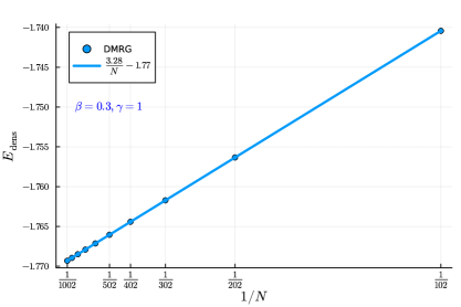
The relative percentage difference between the bulk part of the energy density obtained from Bethe Ansatz and is and the relative percentage difference between the boundary and impurity part of the energy density is .
We show for more representative cases of model parameter and the extraction of boundary and bulk part of the energy density by plotting the energy density for various values of in Fig.18.

C.1 Hermitian limit
When either or is set to zero, the model considered here reduces to the Hermitian case studied in [44] with equal strength of boundary couplings at the two ends of the spin chain. Here, we consider the case when is set to zero and analyze the accuracy of DMRG calculation using ITensor library [36].
We compute the ground state energy for various values of and extract the boundary and bulk part of the energy density. We notice that the bulk part of the energy density obtained from DMRG and Bethe Ansatz in thermodynamic limit have relative difference in order of whereas the boundary part which get contribution from both the open boundary condition and the presence of impurities suffer from finite size effect and hence the difference between the result obtained from two method is relatively larger as shown in Fig.19.
As shown in the first figure of Fig.(18), for the Hermitian case of and , the energy density in thermodynamic limit is extracted by fitting energy density for various values of . We find that the relative error between the Bethe Ansatz and DMRG result for bulk part of the energy density is and the boundary part of the energy density is . This shows that the relative errors in boundary and bulk part of the energy density for Hermitian case is similar to the ones for non-Hermitian case. This shows that the non-Hermitian DMRG implemented in ITensor library [36] used by turning on the ishermitian=false flag works equally well compared to the Hermitian DMRG implemented in ITensor library.