Spinning Black Binaries in de Sitter space
Abstract
We construct stationary, rotating black binaries in general relativity with a positive cosmological constant. We consider identical black holes with either aligned or anti-aligned spins. Both cases have less entropy than the corresponding single Kerr/Schwarzschild de Sitter black hole with the same total angular momentum and cosmological horizon entropy. Our solutions establish continuous non-uniqueness in general relativity without matter. They also provide initial data for the spinning binary merger problem (when orbital angular momentum is added).
Introduction.
A single black hole in isolation is an unchanging, time-independent gravitational object. But can two or more black holes exist in such a state of stationary equilibrium? This question has been around since the early days of general relativity. Early work by Bach and Weyl [1], later generalized by Israel and Khan [2] found multi-black hole solutions that were static, but contained unphysical conical singularities. Indeed, several theorems [3, 4, 5] preclude the existence of static, asymptotically flat multi black holes. With the addition of electric charge, a well-known multi-black hole solution was found by Majumdar and Papapetrou [6, 7], but these solutions require that the black holes be maximally charged, which is unrealistic. Multi black holes were also found in more exotic situations, such as higher-dimensional spacetimes with compact directions [8].
A natural consideration that was not included above is the effect of rotation. While orbital rotation breaks stationarity due to the emission of gravitational waves, spin-spin interactions [9] do not. Notably, spin-spin interactions are a key ingredient to molecular stability [10, 11, 12, 13]. Newtonian attraction scales with distance as , while spin-spin interaction scales as and therefore might have a dominant role at smaller distances. Nevertheless, all known asymptotically flat, stationary black binaries are singular, even those that maximize spin-spin repulsion (see e.g. [14, 15, 16, 17, 18, 19, 20, 21, 22, 23, 24, 25, 26]), though the existence of singularity-free spinning binaries has not been ruled out by any theorem. We do mention here that with the addition of a massive complex scalar field, the scalar pressure together with the spin-spin can balance a spinning binary of hairy black holes [27].
What about the inclusion of a positive cosmological constant ()? After all, this ingredient explains the accelerated expansion of the Universe [28, 29, 30, 31, 32], at least according to the -Cold Dark Matter (CDM) model. With a positive cosmological constant, it was recently found that non-rotating black binary solutions do indeed exist [33]. These solutions are called de Sitter black binaries. These binaries exist because the expansion from the cosmological constant balances out the mutual attraction of the black holes, and their existence could be anticipated from Newton-Hooke analysis [33]. However, this configuration is unstable, as any perturbation would cause the black holes to merge or fly apart.
In this Letter, we add rotation to the de Sitter binaries found in [33], study their properties, and discuss the prospect that spin-spin interactions can stabilize the binaries. For simplicity, we take the individual black holes to be identical and focus on the cases where the spin axes are aligned or anti-aligned, which happens to also be the situations with the strongest spin-spin interaction.
Our results are also of mathematical interest, as they establish continuous non-uniqueness of de Sitter black holes, in contrast to the asymptotically flat case [34, 35, 36, 37, 38, 39, 40, 41, 42, 43, 44].
Newton-Hooke.
Some de Sitter binaries can be described by Newton-Hooke analysis [33], which we review here with the inclusion of spin-spin interactions. We adopt geometrized units .
Consider black holes with masses , positions , and spin vectors , . Including a gravitational force, cosmological Hooke’s law, and dipolar spin-spin interactions, Newton’s second law becomess
| (1) | ||||
for , de Sitter radius , and . Stationary solutions exist when .
Consider now the case with two equal mass black holes separated by a distance , aligned along the -axis, with their spins also aligned along the -axis: , and . Take the symmetric cases with (repulsive spin-spin force) or (attractive spin-spin force). Then (1) admits stationary spinning binary solutions when , which implies
| (2) |
In deriving the above, we discarded terms. We also expressed the mass and spin of the test body in terms of the temperature and angular velocity of a Kerr black hole, so that
| (3) | ||||
For vanishing spin, , (2) yields , where is the Schwarzschild radius of the particles, in agreement with [33]. The equilibrium condition (2) can fall within the regime of validity of Newton-Hook theory, which occurs when (i.e. large ).
With nonzero spin, , an inspection of (2) for a given (large) shows that is a monotonically decreasing function of . Moreover, the curve for the aligned binary () is always below the curve for the anti-aligned case (). This agrees with expectations as spin-spin forces are repulsive for aligned spins, so the black holes need to be closer apart to remain in equilibrium (for fixed gravitational and cosmological forces). The opposite is true for anti-aligned spins. Our numerical (anti-)aligned spinning solutions of de Sitter general relativity will match this behaviour.
Numerical construction.
Now we construct spinning de Sitter binaries using numerical relativity. We use the Einstein-DeTurck method [45] (see [46, 47] for a review), which first involves the selection of a reference metric which has the same causal (regularity, horizon, and asymptotic) structure and, usually, the same symmetries as the solution we seek.
Our reference metric is based on the one used in [33], which is a carefully chosen combination of the Bach-Weyl solution with two identical black holes [1, 2, 48] and the static patch of de Sitter space. Like the reference metric in [33], ours has a symmetry, temporal and azimuthal Killing vectors and , two black hole horizons, and a cosmological horizon. Our main modification is the addition of a cross term that introduces the angular velocities () to the black holes in a frame where the de Sitter horizon is not rotating. The symmetry forces the spin axes of the binaries to be aligned or anti-aligned. Further details on the reference metric can be found in the Supplementary Material.
With a reference metric, we then solve the Einstein-DeTurck equation
| (4) |
where and are the metric and its Ricci tensor, , and is the Christoffel connection. Unlike the Einstein equation (without proper gauge fixing), the equation (4) is elliptic [45, 46, 49, 47], and yields a well-posed boundary problem with suitable boundary conditions. In our case, boundary conditions are set by regularity and symmetry requirements. The aligned and anti-aligned cases have the same boundary conditions except at the symmetry plane, where the metric component has Neumann and Dirichlet boundary conditions, respectively.
A solution to (4) solves the Einstein equation only when (the solution will then be in the gauge ). In certain cases, solutions to the Einstein-DeTurck equation are guaranteed to satisfy [49, 50]. However, there are no such guarantees when . Fortunately, ellipticity guarantees local uniqueness. That is, solutions with cannot be arbitrarily close to those with , and thus we can monitor the norm to verify that our numerical discretization converges in the continuum to a true Einstein solution (see Supplementary Material).
Results.
With our symmetry requirements, the rotating de Sitter binaries form a two-parameter family. Numerically, we take these parameters to be the horizon temperature and angular velocity . Because scanning the full parameter space is computationally expensive, we leave a thorough sweep to future work. Instead we focus our attention on solutions with a fixed temperature , and varying . Note that the Newton-Hooke regime occurs for (i.e. very small black holes).
In Fig. 1, we show the Komar angular momentum of one of the black holes versus its angular velocity . The highest angularity velocity we have reached is . We see no evidence of pathologies or singularities (see Supplementary Material for curvature invariants), so it is possible that these binaries exist for higher (however, it cannot be ruled out that solutions stop existing at a critical due to a lack of bound states).
We show both aligned and anti-aligned results, but they do not differ much. We see that the angular momentum increases with angular velocity. If solutions exist for higher , we would expect that the angular momentum will reach a maximum, as the same occurs for constant-temperature Kerr de Sitter black holes. A polynomial extrapolation gives a peak around 111In a forthcoming publication [DSW-chargedBinary], we construct charged de Sitter binaries, and we see a maximum charge as the electric potential increases..

We now discuss the proper distance along the symmetry axis between the black hole horizons as a function of . This is shown in Fig. 2 for a temperature that seems sufficiently large to expect qualitative matching with Newton-Hooke expectations. We see that, in agreement with the analysis of the Newton-Hooke relation (2), by increasing spin the black holes move closer together with the aligned binary always having a smaller distance.

We now discuss the thermodynamics of the system. In our case, the first law of black hole mechanics reads [52]
| (5) |
where is the temperature of the cosmological horizon, and is its entropy. We checked that our data obeys this law to within .
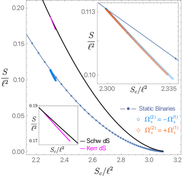
In Fig. 3, we show the total black hole entropy against the cosmological horizon entropy [52]. Again, we are only showing the spinning de Sitter binaries for the constant temperature . For reference, we also included the corresponding values for Schwarzschild de Sitter, Kerr de Sitter, and the static binaries from [33]. In the Kerr case, we only show black holes with the same total angular momentum as the aligned de Sitter binaries. The anti-aligned binaries have zero total angular momentum, so should be compared with Schwarzschild and the static binaries. We see that in all cases, the spinning binaries have less entropy than the corresponding Schwarzschild or Kerr black holes, and so do not dominate the microcanonical ensemble.
From a dynamical perspective, the cosmological horizon entropy does not necessarily stay constant during evolution. But, both horizons satisfy a second law, so it cannot decrease during evolution. We note that our maximal entropy in Fig. 3 is monotonically decreasing with . That is, the maximum entropy is larger than any entropy for . This suggests that the endpoint that maximizes the entropy is indeed the Schwarzschild de Sitter black hole and also suggests its stability. Similar arguments can be made in asymptotically flat space, where energy and angular momentum can be radiated to infinity, and hence are not conserved during evolution.
Conclusions.
We constructed the first examples of stationary, spinning black binary solutions of general relativity with a positive cosmological constant where the gravitational, cosmological and spin-spin interactions combine to produce an equilibrium configuration. We have found these solutions well away from the regime where Newton-Hooke theory is valid, but the properties of our binaries match the Newton-Hooke expectations.
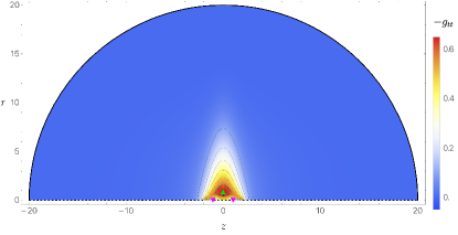
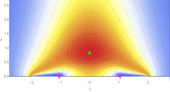
We point out that, like in [33], the available uniqueness theorems [53, 54, 55, 56] do not actually forbid the existence of these de Sitter binaries. This is largely because such theorems make assumptions about the level sets of the gauge-invariant metric component . Fig. 4 shows such level sets for a binary with (other solutions are qualitatively similar). The location of the maximum of is marked by a green triangle. The fact that this maximum is a point in this plot and not a line demonstrates that the assumptions in these theorems are violated (we refer the reader to [33] for a more detailed discussion on this matter).
For completeness, we also show the minima of marked by the two magenta inverted-triangles. These minima take negative values because of the ergoregion around each black hole (where energy and angular momentum can be extracted from the Penrose process or superradiant scattering).
It is clear that black hole uniqueness is strongly violated in de Sitter, unlike in flat space. Indeed, we have an infinite non-uniqueness. For example, in the anti-aligned case, we have a whole continuous two-parameter family of solutions with zero total angular momentum. Therefore, there is no analogous no-hair conjecture [57] for pure gravity with a .
Although the solutions we have found do not dominate the microcanonical ensemble, this does not necessarily mean that they are dynamically unstable. Because spin-spin interactions act on shorter length scales than that of the Newtonian potential, they may provide a mechanism for stabilizing the binary in some regions of parameter space, much like the stability of molecules [10, 11, 12, 13]. It would be interesting to see if this intuition also holds within general relativity, which would require a proper stability analysis of our numerical spinning binaries (or their extensions in the parameter space).
We have left a more thorough search of parameter space to future work. This could include higher angular velocities as well as a sweep over the full 2-parameter family. It would also be interesting to drop the symmetry restrictions and consider unequal black holes with unequal spins. In the case where one of the black holes is much smaller than the other, the Mathisson-Papapetrou-Dixon’s formalism [58, 59, 60, 61, 62, 63, 9] can be used. Work in this direction is underway.
Finally, we note that our solutions have spin but no orbital angular momentum. Adding orbital angular momentum will also create quadrupole moments that emit gravitational radiation and hence, the system will not be stationary. Nevertheless, our solutions can provide initial data that satisfy the elliptic constraint equations of the time evolution problem, that ultimately leads to the black hole binary merger and associated gravitational (and electromagnetic) wave emission.
Acknowledgements.
Acknowledgments.
O.D. acknowledges financial support from the STFC “Particle Physics Grants Panel (PPGP) 2018” Grant No. ST/T000775/1 and PPGP 2020 grant No. ST/X000583/1. O.D.’s research was also supported in part by the YITP-ExU long-term workshop Quantum Information, Quantum Matter and Quantum Gravity (QIMG2023), Yukawa Institute for Theoretical Physics, Kyoto Univ., where part of this work was completed. J. E. S. has been partially supported by STFC consolidated grant ST/T000694/1. The authors acknowledge the use of the IRIDIS High Performance Computing Facility, and associated support services at the University of Southampton, for the completion of this work.
Supplementary Material
Appendix A Metric Ansatz for Spinning Black Binaries in de Sitter
In the Einstein-DeTurck formalism, (4) requires a reference metric which has the same casual (asymptotic and horizon) structure and, whenever possible, also the same symmetries as the solution we seek. We will follow the same procedure in [33] to obtain the reference metric, making a few modifications to accommodate spin.
The reference metric in [33] was built from a careful combination of the Bach-Weyl [1] (i.e., the Israel-Khan solution [2] with two black holes) and de Sitter space. The Bach-Weyl solution is a closed form, asymptotically flat solution of the Einstein equation that consists of two non-spinning black holes held together by a conical singularity. The overall strategy is to combine this singular binary with the de Sitter horizon in hopes of finding a de Sitter solution with a conical singularity, and then remove the conical singularity.
The Bach-Weyl solution is usually written in Weyl coordinates because the resulting Einstein equation in this gauge can be expressed in an integrable form. These coordinates have a “rod-structure” so that the coordinate line includes both inner and outer segments of the symmetry axis as well as the black hole horizons. This rod-structure is inconvenient for numerical purposes, largely because it introduces more coordinate singularities and makes the application of boundary conditions difficult. Instead, in [33], a transformation
| (6) |
was used to map both horizons, as well as the outer and inner segments of the axis into the four sides of a coordinate rectangle . The Bach-Weyl solution [1, 2] then takes the form [33]
| (7) |
where is an arbitrary dimensionful length scale that we have introduced for later use in de Sitter, and
| (8) | ||||
All functions , , , , and are smooth and positive definite in the domain. vanishes at (asymptotic infinity), and is positive and smooth otherwise. The solution is parametrized by .
To eventually accommodate a cosmological horizon, we also consider the polar Weyl coordinates defined by:
| (9) |
where the Bach-Weyl solution [1, 2] takes the form [33]
| (10) |
with
| (11) | ||||
Note that and approach unity when , where the spacetime becomes asymptotically flat.
Now we separately consider de Sitter space, which can be written in isotropic coordinates [33]
| (12) |
where is the de Sitter radius . In these coordinates, the de Sitter horizon has a constant temperature of . In (12), as in (10), is a gauge parameter that simply scales the radial coordinate .
The form (12) for de Sitter space is suggestively similar to the Bach-Weyl solution (10) in polar Weyl coordinates. Aside from some factors of and (which approach unity at large ), the only differences are that de Sitter in isotropic coordinates has an overall conformal factor of and a factor of in the term whose zero defines the de Sitter horizon. This effectively constrains the coordinate in our integration domain to . We will make use of these similarities below.
Now we can form a reference metric as was done in [33]. To do so note that from (6) and (9), we can find an explicit coordinate transformation between the coordinates and the polar Weyl coordinates:
| (13a) | ||||
| (13b) | ||||
which is needed in what follows.
With these ingredients in place, we can finally describe our reference metric:
| (14) |
with several functions that appear in theses metrics defined in (8) or (A). We will describe the remaining functions further below. The equality between the first and second lines of (A) (here and in the remainder of this section) is understood to be through the coordinate transformation (13). We will use coordinates in the region near the black holes and inner segment of the axis, and the coordinates near the cosmological horizon. The DeTurck metric (A) is a simple upgrade of the static DeTurck reference metric (B5) of [33] where we have simply introduced a term to accommodate the spins of the black holes. More concretely, we have simply taken (B5) of [33] and made the replacement (which also introduces a new function defined below). This reference metric depends on four parameters, and whose physical interpretation is given below.
We only made four changes to the Bach-Weyl (Israel-Khan) solution to arrive at the reference metric (A). The first is the inclusion of a conformal factor to enable the matching to de Sitter spacetime (12) in isotropic coordinates in the far-region. The second is the inclusion of a function in the term with a conical parameter that we will adjust to remove any conical singularities. This is achieved with the choices
| (15) |
The third change is the inclusion of a factor of in the term which introduces a cosmological horizon at ( is a complicated function that will be given further below in (17)). The fourth change is the replacement where must satisfy but can otherwise be freely chosen. We choose
| (16) |
This fourth change introduces an angular velocity at the horizons (which is given by the novel parameter ) but leaves the cosmological horizon (where vanishes) with zero rotation.
We have some freedom to choose the function , but the choice is delicate [33]. For numerical reasons, we want to be smooth both in and coordinates. The DeTurck method further requires that preserves the regularity of both the black hole and cosmological horizons [45, 46, 47]. In addition, to aid in finding a solution using a Newton-Raphson algorithm, it would be convenient to also choose to match physical expectations in certain limits. Specifically, we expect that when the cosmological horizon is large compared to other length scales (i.e. ), the spacetime near the cosmological horizon should approach de Sitter and the spacetime closer to the origin should be approximately described by the Bach-Weyl solution (when and ). As detailed in [33], these requirements are achieved if we choose to be [33]
| (17) |
where and are any smooth, positive definite functions that agree with and , respectively at . To choose and , we first take the expressions for and as written in (A), and treat them as functions and . We then set and similarly for . Note that we cannot use a choice like as it is not smooth in the coordinates at .
The reference metric (A) is parametrized by , , and . This metric describes a solution that is everywhere regular when the conical parameter to be given by (15), with black hole horizons at . These are Killing horizons generated by the Killing vector field , i.e. (where we use the fact that and ). The temperature and angular velocity are given by
| (18) |
where and . Note that because of the overall factor of in the metric, and as expressed here are dimensionless. Any and that give the same are physically equivalent. Effectively, is a gauge parameter that only sets an overall scale (it fixes the cosmological horizon location to be at ) and then fixes the black hole temperature. Solutions described by (A) also have a cosmological horizon at (where vanishes) with temperature and angular velocity . This is generated by the Killing vector field , i.e. . Note that, unlike the event horizon, the cosmological horizon has vanishing angular velocity. The reference metric therefore only has two physical parameters, and (or and ).
With a reference metric, we can finally write our metric ansatz for the spinning binary in de Sitter, which is essentially the most general ansatz compatible with the symmetries of the problem:
| (19) |
where are unknown functions of and are unknown functions of . The known functions, already present in (A) and defined in (8) or (A), should be treated as scalars, transforming between coordinate systems as (13). Note that when we set (and similarly for the associated set of tilde functions ), we recover the DeTurck reference metric (A). The choice of our treatment of the factor allows us to more easily recover the static results [33] in the limit .
Most of the boundary conditions are determined by regularity, and we refer readers to Section V of the review [47] for a detailed discussion of such boundary conditions. Many of these are set by including factors of , , and (and similar factors of , , and into the metric ansatz. The reflection plane at () deserves a few further comments. Our reference metric is even about this surface, which agrees with the desired solutions with aligned spins, for which we demand Neumann boundary conditions. For the anti-aligned case, we take the same boundary conditions except for (), for which we choose a Dirichlet condition. The fact that the reference metric does not itself satisfy this condition does not lead to any contradictions. This is indeed not a problem since this is happening at an axis of symmetry (not at a boundary of the spacetime) and the reference metric still has well defined parity (moreover, one explicitly checks that the de Turck norm indeed vanishes along this axis even with the Neumann boundary conditions).
We supplement the boundary conditions by a set of patching conditions to join the two different coordinate systems together. We defer a discussion of patching to the next section.
For fixed cosmological constant, our solutions are physically parametrised by and , but our solutions are parametrised by four parameters: , , , . is set according to (15) to remove conical singularities, is uniquely determined by a choice of , but any combination of our parameters and that give the same black hole temperature are physically equivalent. After some trial and error, we find good numerical results by fixing and using and to parametrize the solutions.
Our (aligned or anti-aligned) spinning de Sitter binaries are thus a 2-parameter family of solutions parametrized by and . Any combination of and that give the same black hole temperature are physically equivalent. To collect our numerical data, we typically have fixed and used and to parametrize our solutions. We have tried different values of , but after trial and error, this value typically generated the best numerical results.
Appendix B Patching and Numerical Methods
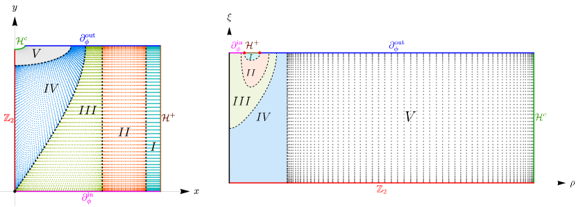
In this section, we explain how we partition the domain of integration using patching techniques (reviewed e.g. in [47]). The solution we seek contains five boundaries: the inner segment of the axis (), the black hole horizon (), the outer segment of the axis (), the cosmological horizon (), and the plane of symmetry. Near the black hole event horizon we use coordinates, while near the cosmological horizon we use coordinates, and these coordinates at patched together.
For the results presented in this Letter, we used a total of five patches , ,, and with each of these having four boundaries: see Fig. 5. Patches and are defined in coordinates, and patch in coordinates. The patching boundary (dashed line in Fig. 5) between patches and is given by constant , and between patches and it is given by constant . The patching boundary between patches and is given by . Finally, the patching boundary between patch and patch is given by .
We fix the grid parameters , and by:
| (20) |
We apply the numerical methods detailed in [47], and discretize each of our patches on a Chebyshev-Gauss-Lobatto grid using transfinite interpolation and pseudospectral collocation, for a total grid size of . For , the associated grid points are explicitly displayed in Fig. 5, using a different colour code for each patch. After discretization, the Newton-Raphson equation and boundary conditions are solved with LU decomposition, using the (static) solution of [33] as a first starting seed.
Appendix C Further results
Let us review the Kerr de Sitter black hole in order to make comparisons with the spinning binaries. We begin by introducing the parameters and , where and are the horizon radius and cosmological horizon radius, and is the rotation parameter. Then in a frame with a non-rotating cosmological horizon, the temperature, entropy, angular velocity, and angular momenta of the event () and cosmological () horizons of the Kerr-dS (KdS) black hole are:
| (21) |
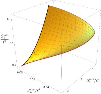
Regular Kerr-dS black holes exist for and where is the value of at extremality where . In the left panel of Fig. 6, we display the microcanonical phase diagram with the Kerr-dS black hole family. This plot displays the full Kerr-dS family of solutions. The black line () describes the Schwarzschild-dS solution, the red line describes the extremal Kerr-dS family () and the grey curve describes Kerr-dS black holes in the Nariai limit (i.e. ).
To produce the microcanonical phase diagram displayed in Fig. 3 of the main text, we had to find the corresponding Kerr-dS (or Schwarzschild-dS) solution with the same and same angular momentum as the spinning binary. For that, we used (C) to find the matching Kerr-dS parameters , and then used these to find the event horizon entropy of this Kerr-dS black hole. This generates the magenta curve in Fig. 3 of the main text or the cyan and magenta curves in the left panel of Fig. 3 (note that for the cyan curve one has , i.e. it describes Schwarzschild-dS black holes) that are also displayed in the left panel of Fig. 6 (the cyan curve on top of the black curve is barely seen since it has very small length). As it is clear from Fig. 3 in the main text, the 2-parameter families of regular (anti-)aligned spinning binaries are described by surfaces that are well below the Kerr-dS surface of Fig. 6 (for values of and where they co-exist).
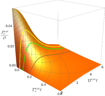
In the main text, we pointed out that for Kerr-dS black holes with fixed temperature, the Komar angular momentum first increases with till it reaches a maximum, and then decreases as increases further. This is explicitly shown in the right panel of Fig. 6 where we plot as a function of and and display three families with constant (yellow, green, brown curves); note that Ker-dS exists for higher values of temperature and angular velocity than those shown.
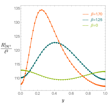
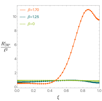
We have designed our numerical code such that the binary solutions are parametrized by the black hole temperature and angular velocity. In particular, some of the solutions we present have constant temperature and with . We stopped at because it becomes increasingly more difficult to find numerical solutions with higher . This occurs because some of the functions start developing very large gradients and/or a hierarchy of scales between different regions of the integration domain. However, do not find no evidence for the appearance of curvature singularities beyond . One such curvature invariant that we monitored is the pullback of the Ricci curvature into the black hole () and cosmological horizons (), which are shown in the left and right panels of Fig. 7, for three different values of . These quantities remain clearly finite as grows which suggests that our binaries should exist for even higher values of without developing curvature singularities.
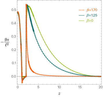
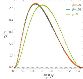
An important gauge invariant quantity of the binary system is the time-time component of the metric . In the left panel of Fig. 8 we plot as a function of the Weyl coordinate along the axis that connects the two black holes (i.e. with Weyl coordinate ) and that contains the inner -axis (), black hole horizon () and outer -axis () for anti-aligned binaries with for three different values of . We first notice the existence of an ergoregion with . As expected, we see that this ergoregion is absent for , and the minimum of becomes more negative as increases. One also finds that becomes considerably more spiked around its local maximum outside the black hole horizon (i.e. just above ) and then decays faster with as increases. This partially justifies why it becomes increasingly more difficult to find our numerical solutions as grows. But it is important to note that this does not imply the development of any pathology. Indeed, if instead of the (gauge dependent) coordinate , we plot as a function of the (gauge invariant) proper length along the outer -axis, as we do in the right panel of Fig. 8, one finds that the qualitative behaviour of the curve (in particular, its width) does not change significantly as increases. Anti-aligned spinning binaries with have similar qualitative behaviour.
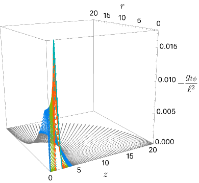
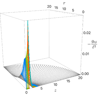
To have a more holistic illustration of how our solutions look like, (besides Fig. 4 in the main text) in Figs. 910 we display the two metric functions and (that are gauge invariant since and are Killing vector fields) as a function of the original cylindrical Weyl coordinates for two representative aligned spinning binaries with black hole temperature and angular velocity (Fig. 9) and (Fig. 10). The system is symmetric about , i.e. (the minus sign holds only for the component in the anti-aligned binary) and thus we just display the solution for . The five different colours represent the five distinct patches that we use and the colour code is the same one displayed in Fig. 5. Note that, as required, one always has a smooth transition between patches. Anti-aligned spinning binaries with have similar qualitative behaviour.
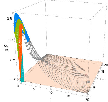
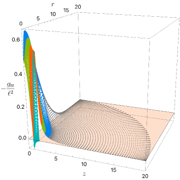
Recall that in this cylindrical Weyl coordinate chart , we have a “rod structure” where the rotation axis and the black hole horizons are all located at . More concretely, at , the black horizon lies in the region and thus, the norm of the horizon generator vanishes here (not plotted). The ergoregion (where ) is also along this segment at but extends for in a neighbourhood of this rod. Figs. 910 indeed show that is negative in these ergoregions and that the negative absolute minimum of (that is at as better pinpointed by the magenta inverted triangles in Fig. 4) increases as increases. Moreover, still at , the inner segment of the axis between the black holes is in the region and the outer segments of the axis are in and : not shown (see [33]), vanishes in these segments. The solution has a cosmological horizon at (with temperature ) where vanishes (since this horizon is generated by with ) as clearly identified in the left panels of Figs. 910 .
In the right panels of Figs. 910 we plot . This function vanishes everywhere when . When the components of the binary are spinning, vanishes at along the inner and outer segments of the axis. It also vanishes at the cosmological horizon since , but is otherwise non-zero. In particular, it is non-vanishing at along inside of which it attains its maximum value, and this maximum value increases as increases. Note that is an even function of for aligned spinning binaries (the case that is shown in Figs. 910), but is an odd function of in the anti-aligned binary case (not shown).
Appendix D Convergence Tests
In this section, we show that the norm of the DeTurck vector vanishes in the continuum limit, as expected for a solution of the Einstein-DeTurck equation that is not a Ricci soliton (i.e. that is instead a true solution to the Einstein equation). Additionally, we find exponential convergence, which is consistent with the use of Chebyshev pseudospectral collocation methods.
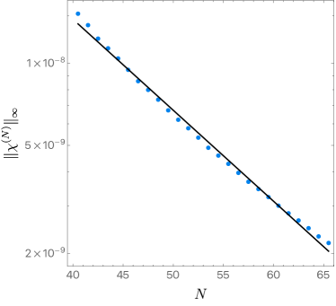
Let be computed on a (5-patched) grid with spectral collocation points. For concreteness, we take as given in (15), , and . In Fig. 11 we show as a function of in a -plot. The solid black line shows the best -fit to a straight line in the -plot, and yields
| (22) |
The exponential trend is clear and confirms that the Einstein-DeTurck solution is converging to a true solution of the Einstein equation (and not to a Ricci soliton with finite ).
References
- [1] R. Bach and H. Weyl, “New solutions to Einstein’s equations of gravitation. B. Explicit determination of static, axially symmetric fields (By Rudolf Bach). With a supplement on the static two-body problem (By Hermann Weyl). [Republication of: R. Bach and H. Weyl, Mathematische Zeitschrift 13 (1922) 134] ,” Gen Relativ Gravit 44 (2012) 817.
- [2] W. Israel and K. A. Khan, “Collinear particles and bondi dipoles in general relativity,” Il Nuovo Cimento (1955-1965) 33 no. 2, (Jul, 1964) 331–344.
- [3] W. Israel, “Event horizons in static vacuum space-times,” Phys. Rev. 164 (1967) 1776–1779.
- [4] D. C. Robinson, “A simple proof of the generalization of Israel’s theorem.,” General Relativity and Gravitation 8 no. 8, (Aug., 1977) 695–698.
- [5] G. L. Bunting and A. K. M. Masood-Ul-Alam, “Nonexistence of multiple black holes in asymptotically Euclidean static vacuum space-time.,” General Relativity and Gravitation 19 no. 2, (Feb., 1987) 147–154.
- [6] S. D. Majumdar, “A class of exact solutions of Einstein’s field equations,” Phys. Rev. 72 (1947) 390–398.
- [7] A. Papapetrou, “A Static solution of the equations of the gravitational field for an arbitrary charge distribution,” Proc. Roy. Irish Acad.(Sect. A) A51 (1947) 191–204.
- [8] M. Astorino, R. Emparan, and A. Viganò, “Bubbles of nothing in binary black holes and black rings, and viceversa,” JHEP 07 (2022) 007, arXiv:2204.09690 [hep-th].
- [9] R. M. Wald, “Gravitational spin interaction,” Phys. Rev. D 6 (1972) 406–413.
- [10] N. Bohr, “On the constitution of atoms and molecules, part i,” Philosophical Magazine 26 (1913) 1.
- [11] N. Bohr, “On the constitution of atoms and molecules, part ii, systems containing only a single nucleus,” Philosophical Magazine 26 (1913) 476.
- [12] N. Bohr, “On the constitution of atoms and molecules, part iii, systems containing several nuclei,” Philosophical Magazine 26 (1913) 857.
- [13] A. Svidzinsky, M. Scully, and D. Herschbach, “Bohr’s molecular model, a century later,” Physics Today 67 no. 1, (01, 2014) 33–39.
- [14] Z. Perjés, “Solutions of the coupled einstein-maxwell equations representing the fields of spinning sources,” Phys. Rev. Lett. 27 (Dec, 1971) 1668–1670.
- [15] W. Israel and G. A. Wilson, “A class of stationary electromagnetic vacuum fields,” J. Math. Phys. 13 (1972) 865–871.
- [16] J. B. Hartle and S. W. Hawking, “Solutions of the Einstein-Maxwell equations with many black holes,” Commun. Math. Phys. 26 (1972) 87–101.
- [17] A. Tomimatsu and H. Sato, “New Exact Solution for the Gravitational Field of a Spinning Mass,” Phys. Rev. Lett. 29 (1972) 1344–1345.
- [18] D. Kramer and G. Neugebauer, “The superposition of two kerr solutions,” Physics Letters A 75 no. 4, (1980) 259–261.
- [19] G. Neugebauer, “Relarivistic gravitational fields of rotating bodies,” Physics Letters A 86 no. 2, (1981) 91–93.
- [20] H. Stephani, D. Kramer, M. MacCallum, C. Hoenselaers, and E. Herlt, Exact Solutions of Einstein’s Field Equations. Cambridge Monographs on Mathematical Physics. Cambridge University Press, 2 ed., 2003.
- [21] V. S. Manko and E. Ruiz, “Exact solution of the double-kerr equilibrium problem,” Classical and Quantum Gravity 18 no. 2, (Jan, 2001) L11.
- [22] C. A. R. Herdeiro and C. Rebelo, “On the interaction between two Kerr black holes,” JHEP 10 (2008) 017, arXiv:0808.3941 [gr-qc].
- [23] V. S. Manko, E. D. Rodchenko, E. Ruiz, and B. I. Sadovnikov, “Exact solutions for a system of two counter-rotating black holes,” Phys. Rev. D 78 (2008) 124014, arXiv:0809.2422 [gr-qc].
- [24] V. S. Manko and E. Ruiz, “Metric for two equal Kerr black holes,” Phys. Rev. D 96 no. 10, (2017) 104016, arXiv:1702.05802 [gr-qc].
- [25] V. S. Manko and E. Ruiz, “Metric for two arbitrary Kerr sources,” Phys. Lett. B 794 (2019) 36–40, arXiv:1806.10408 [gr-qc].
- [26] V. S. Manko and E. Ruiz, “Equatorially symmetric configurations of two Kerr-Newman black holes,” Phys. Rev. D 105 no. 2, (2022) 024036, arXiv:2011.04313 [gr-qc].
- [27] C. A. R. Herdeiro and E. Radu, “Two Spinning Black Holes Balanced by Their Synchronized Scalar Hair,” Phys. Rev. Lett. 131 no. 12, (2023) 121401, arXiv:2305.15467 [gr-qc].
- [28] Supernova Cosmology Project Collaboration, S. Perlmutter et al., “Discovery of a supernova explosion at half the age of the Universe and its cosmological implications,” Nature 391 (1998) 51–54, arXiv:astro-ph/9712212.
- [29] Supernova Search Team Collaboration, A. G. Riess et al., “Observational evidence from supernovae for an accelerating universe and a cosmological constant,” Astron. J. 116 (1998) 1009–1038, arXiv:astro-ph/9805201.
- [30] Supernova Cosmology Project Collaboration, S. Perlmutter et al., “Measurements of and from 42 high redshift supernovae,” Astrophys. J. 517 (1999) 565–586, arXiv:astro-ph/9812133.
- [31] A. Wright, “It’s a mystery,” Nature Physics 7 no. 11, (Nov, 2011) 833–833.
- [32] Planck Collaboration, P. A. R. Ade et al., “Planck 2013 results. XVI. Cosmological parameters,” Astron. Astrophys. 571 (2014) A16, arXiv:1303.5076 [astro-ph.CO].
- [33] O. J. C. Dias, G. W. Gibbons, J. E. Santos, and B. Way, “Static Black Binaries in de Sitter Space,” Phys. Rev. Lett. 131 no. 13, (2023) 131401, arXiv:2303.07361 [gr-qc].
- [34] J. E. Chase, “Event horizons in static scalar-vacuum space-times,” Commun. Math. Phys. 19 (1970) 276.
- [35] R. Penney, “Axially Symmetric Zero-Mass Meson Solutions of Einstein Equations,” Phys. Rev. 174 (1968) 1578–1579.
- [36] J. D. Bekenstein, “Transcendence of the law of baryon-number conservation in black hole physics,” Phys. Rev. Lett. 28 (1972) 452–455.
- [37] J. D. Bekenstein, “Nonexistence of baryon number for static black holes,” Phys. Rev. D5 (1972) 1239–1246.
- [38] J. D. Bekenstein, “Nonexistence of baryon number for black holes. ii,” Phys. Rev. D5 (1972) 2403–2412.
- [39] C. Teitelboim, “Nonmeasurability of the quantum numbers of a black hole,” Phys. Rev. D5 (1972) 2941–2954.
- [40] J. B. Hartle, Magic Without Magic. edited by J. Klauder, Freeman, San Francisco, 1972.
- [41] M. Heusler, “A No hair theorem for selfgravitating nonlinear sigma models,” J. Math. Phys. 33 (1992) 3497–3502.
- [42] J. D. Bekenstein, “Novel ’no scalar hair’ theorem for black holes,” Phys. Rev. D51 (1995) 6608–6611.
- [43] J. D. Bekenstein, “Black hole hair: 25 - years after,” in 2nd International Sakharov Conference on Physics, pp. 216–219. 5, 1996. arXiv:gr-qc/9605059.
- [44] D. Sudarsky, “A Simple proof of a no hair theorem in Einstein Higgs theory,,” Class. Quant. Grav. 12 (1995) 579–584.
- [45] M. Headrick, S. Kitchen, and T. Wiseman, “A New approach to static numerical relativity, and its application to Kaluza-Klein black holes,” Class. Quant. Grav. 27 (2010) 035002, arXiv:0905.1822 [gr-qc].
- [46] T. Wiseman, Numerical construction of static and stationary black holes. in Black Holes in Higher Dimensions, CUP 2012, Ed. Gary T. Horowitz, 2011. arXiv:1107.5513 [gr-qc]. http://inspirehep.net/record/920553/files/arXiv:1107.5513.pdf.
- [47] O. J. C. Dias, J. E. Santos, and B. Way, “Numerical Methods for Finding Stationary Gravitational Solutions,” Class. Quant. Grav. 33 no. 13, (2016) 133001, arXiv:1510.02804 [hep-th].
- [48] R. Emparan and E. Teo, “Macroscopic and microscopic description of black diholes,” Nucl. Phys. B 610 (2001) 190–214, arXiv:hep-th/0104206.
- [49] P. Figueras, J. Lucietti, and T. Wiseman, “Ricci solitons, Ricci flow, and strongly coupled CFT in the Schwarzschild Unruh or Boulware vacua,” Class. Quant. Grav. 28 (2011) 215018, arXiv:1104.4489 [hep-th].
- [50] P. Figueras and T. Wiseman, “On the existence of stationary Ricci solitons,” Class. Quant. Grav. 34 no. 14, (2017) 145007, arXiv:1610.06178 [gr-qc].
- [51] In a forthcoming publication [DSW-chargedBinary], we construct charged de Sitter binaries, and we see a maximum charge as the electric potential increases.
- [52] G. W. Gibbons and S. W. Hawking, “Cosmological Event Horizons, Thermodynamics, and Particle Creation,” Phys. Rev. D 15 (1977) 2738–2751.
- [53] P. G. LeFloch and L. Rozoy, “Uniqueness of kottler spacetime and the besse conjecture,” Comptes Rendus Mathematique 348 no. 19, (2010) 1129–1132.
- [54] S. Borghini, P. T. Chruściel, and L. Mazzieri, “On the uniqueness of Schwarzschild-de Sitter spacetime,” arXiv:1909.05941 [math.DG].
- [55] D. Katona and J. Lucietti, “Uniqueness of the extremal Schwarzschild de Sitter spacetime,” Lett. Math. Phys. 114 no. 1, (2024) 18, arXiv:2309.04238 [gr-qc].
- [56] D. Katona, “Uniqueness of extremal charged black holes in de Sitter,” arXiv:2403.08467 [gr-qc].
- [57] R. Ruffini and J. A. Wheeler, “Introducing the black hole,” Phys. Today 24 no. 1, (1971) 30.
- [58] M. Mathisson, “Republication of: New mechanics of material systems, acta phys. pol. 6 (1937) 163,” General relativity and gravitation 42 no. 4, (2010) 1011–1048.
- [59] A. Papapetrou, “Spinning test-particles in general relativity. i,” Proceedings of the Royal Society of London. Series A. Mathematical and Physical Sciences 209 no. 1097, (1951) 248–258.
- [60] E. Corinaldesi and A. Papapetrou, “Spinning test-particles in general relativity. ii,” Proceedings of the Royal Society of London. Series A. Mathematical and Physical Sciences 209 no. 1097, (1951) 259–268.
- [61] W. G. Dixon, “Dynamics of extended bodies in general relativity. I. Momentum and angular momentum,” Proc. Roy. Soc. Lond. A 314 (1970) 499–527.
- [62] W. G. Dixon, “The definition of multipole moments for extended bodies,” General Relativity and Gravitation 4 (1973) 199–209.
- [63] W. G. Dixon, “Dynamics of extended bodies in general relativity III. Equations of motion,” Phil. Trans. Roy. Soc. Lond. A 277 no. 1264, (1974) 59–119.