Accelerated Over-Relaxation Heavy-Ball Methods with Provable Acceleration and Global Convergence

Abstract

The heavy-ball momentum method has gained widespread popularity for accelerating gradient descent by incorporating a momentum term. Recent studies have conclusively shown that the heavy-ball method cannot achieve an accelerated convergence rate for general smooth strongly convex optimization problems. This work introduces the Accelerated Over-Relaxation Heavy-Ball (AOR-HB) method, a novel approach that represents the first heavy-ball method to demonstrate provable global and accelerated convergence for smooth strongly convex optimization. The key innovation of the AOR-HB method lies in the application of an over-relaxation technique to the gradient term. This novel approach enables the method to be applied to min-max problems and meet optimal lower complexity bounds. This breakthrough addresses a long-standing theoretical gap in heavy-ball momentum methods and paves the way for developing accelerated methods that transcend the boundaries of convex optimization to non-convex optimization. Numerical experiments validate the effectiveness of the proposed algorithms, with their performance matching that of other leading first-order optimization methods.

1 Introduction

We first consider the unconstrained optimization problem:

$$\min_{x\in\mathbb{R}^{d}}f(x),$$ (1)

where the objective function $f$ is $\mu$-strongly convex and $L$-smooth. Later on we also consider extension to a class of min-max problems (7) with bilinear coupling.

Notation.

$\mathbb{R}^{d}$ is $d$-dimensional Euclidean space with inner product $\langle\cdot,\cdot\rangle$ and the induced norm $\|\cdot\|$. $f:\mathbb{R}^{d}\to\mathbb{R}$ is a differentiable function. We say $f$ is $\mu$-strongly convex function when there exists $\mu>0$ such that

$$f(y)-f(x)-\langle\nabla f(x),y-x\rangle\geq\frac{\mu}{2}\|x-y\|^{2},\quad\forall~{}x,y\in\mathbb{R}^{d}.$$

We say $f$ is $L$-smooth with $L>0$ if its gradient is Lipschitz continuous:

$$\|\nabla f(x)-\nabla f(y)\|\leq L\|x-y\|,\quad\forall~{}x,y\in\mathbb{R}^{d}.$$

The condition number $\kappa_{f}$ is defined as $\kappa_{f}=L/\mu$.

When $f$ is $\mu$-strongly convex and $L$-smooth, the global minimizer $x^{*}$ of problem (1) exists and is unique. The Bregman divergence of $f$ is defined as $D_{f}(y,x):=f(y)-f(x)-\langle\nabla f(x),y-x\rangle$. In particular, $D_{f}(x,x^{*})=f(x)-f^{*}$ as $\nabla f(x^{*})=0$. Various bounds and identities on the Bregman divergence can be found in Appendix A.

Heavy-ball methods and flow.

Over the past two decades, first-order methods, which rely solely on gradient information rather than the Hessian as required by Newton’s method, have gained significant interest due to their efficiency and adaptability to large-scale data-driven applications and machine learning tasks (Bottou et al., , 2018). Among these methods, the gradient descent method is one of the most straightforward and well-established algorithms. However, for ill-conditioned problems, where the condition number $\kappa_{f}\gg 1$, the gradient descent method suffers from slow convergence.

In order to accelerate the gradient descent methods, a momentum term, i.e., a weighted combination of the previous step, was introduced, encouraging the method to move along search directions that utilize not only current but also previously seen information. The heavy-ball (HB) method (also known as the momentum method (Polyak, , 1964)) was in the form of:

$$x_{k+1}=x_{k}-\gamma\nabla f(x_{k})+\beta(x_{k}-x_{k-1}),$$ (2)

where $(\beta,\gamma)$ are constant parameters. Polyak motivated the method by an analogy to a "heavy ball" moving in a potential well defined by the cost function. The corresponding ordinary differential equation (ODE) model is commonly referred to as the heavy-ball flow (Polyak, , 1964):

$$x^{\prime\prime}+\theta x^{\prime}+\eta\nabla f(x)=0,$$ (3)

where $x^{\prime}$ is taking the derivative of $x(t)$ for $t>0$, and $(\theta,\eta)$ are constant parameters.

Non-convergence and non-acceleration of the HB method.

Polyak, (1964) showed under a suitable choice of parameters $(\beta,\gamma)$ in (2): $\beta=\left(\frac{\sqrt{L}-\sqrt{\mu}}{\sqrt{L}+\sqrt{\mu}}\right)^{2}$, $\gamma=\frac{4}{(\sqrt{L}+\sqrt{\mu})^{2}}$, and when $x_{k}$ is sufficiently close to the optimal solution $x^{*}$, $\|x_{k}-x^{*}\|$ converges at rate $\frac{1-\sqrt{\rho}}{1+\sqrt{\rho}}$, where $\rho=\mu/L=1/\kappa$. Polyak’s choice relies on the spectral analysis of the linear system and thus the accelerated rate is only limited to the convex and quadratic objectives and is local for iterates near $x^{*}$. Indeed Lessard et al., (2016) designed a non-convergent example to show that the Polyak’s choice of parameters does not guarantee the global convergence for general strongly convex objective functions.

By changing to an appropriate range of parameters $(\beta,\gamma)$, in Ghadimi et al., (2015); Sun et al., (2019); Saab Jr et al., (2022); Shi et al., (2022), the global linear convergence of the HB method has been established. However, the rate is given by $1-\mathcal{O}(\rho)$ in Shi et al., (2022), which coincides with that of the gradient descent and not the accelerated rate $1-\mathcal{O}(\sqrt{\rho})$.

The absence of acceleration is not due to a technical difficulty in the convergence analysis. Recently, Goujaud et al., (2023) have demonstrated that the HB method provably fails to achieve an accelerated convergence rate for smooth and strongly convex problems. Specifically, for any positive parameters $(\beta,\gamma)$ in equation (2), there exists an $L$-smooth, $\mu$-strongly convex function, and an initialization such that HB fails to converge. Even in the class of smooth and strongly convex quadratic function $f$, the convergence rate is not accelerated; that is, it is $1-\mathcal{O}(\rho)$. Consequently, the HB method, in the form of equation (2), does not offer global and accelerated convergence for general convex functions. For more related works on HB methods, see Appendix B.1.

Main contributions for strongly convex optimization.

We propose a variant of the HB method in the form of

$$x_{k+1} =x_{k}-\gamma(2\nabla f(x_{k})-\nabla f(x_{k-1}))+\beta(x_{k}-x_{k-1}),$$ (4)

$$\gamma =\frac{1}{(\sqrt{L}+\sqrt{\mu})^{2}},\quad\quad\beta=\frac{L}{(\sqrt{L}+\sqrt{\mu})^{2}}.$$

The method (4) can be obtained as a discretization of the HB flow (3) with $\theta=2,\eta=\frac{1}{\mu}$. The most notable yet simple change is using $2\nabla f(x_{k})-\nabla f(x_{k-1})$ not $\nabla f(x_{k})$ to approximate $\nabla f(x)$. Namely an over-relaxation technique is applied to the gradient term. Therefore, we name (4) accelerated over-relaxation heavy-ball (AOR-HB) method. The gradient $\nabla f(x_{k})$ can be re-used and thus essentially only one gradient evaluation is required for one iteration. An equivalent and analysis friendly version is given in (14) where two iterates $(x_{k},y_{k})$ are used.

We rigorously prove that AOR-HB enjoys the global linear convergence with accelerated rate.

Theorem 1.1 (Convergence of AOR-HB method).

Suppose $f$ is $\mu$-strongly convex and $L$-smooth. Let $(x_{k},y_{k})$ be generated by scheme (14) with initial value $(x_{0},y_{0})$ and step size $\alpha=\sqrt{\mu/L}$. Then there exists a non-negative constant $C_{0}=C_{0}(x_{0},y_{0},\mu,L)$ so that we have the accelerated linear convergence

$$f(x_{k+1})-f^{*}+\frac{\mu}{2}\|y_{k+1}-x^{*}\|^{2}\leq C_{0}\left(\frac{2}{2+\sqrt{\mu/L}}\right)^{k},\quad k\geq 1.$$ (5)

Other optimal first-order methods.

To accelerate the HB method, one can introduce either an additional gradient step or a line search step with adequate decay into the algorithm; see Wilson et al., (2021); Siegel, (2019); Chen and Luo, (2021).

Nesterov accelerated gradient (Nesterov, , 1983, page 81) can be viewed as an alternative enhancement of the HB method. Nesterov’s approach calculates the gradient at points that are extrapolated based on the inertial force:

$$x_{k+1} =x_{k}+\beta(x_{k}-x_{k-1})-\gamma\nabla f(x_{k}+\beta(x_{k}-x_{k-1})),~{}\text{with}~{}\beta=\frac{\sqrt{L}-\sqrt{\mu}}{\sqrt{L}+\sqrt{\mu}},\gamma=\frac{1}{L}.$$ (6)

Nesterov devised the method of estimate sequences (Nesterov, , 2013) to prove that (6) achieves the optimal linear convergence rate $1-\mathcal{O}(\sqrt{\rho})$.

The AOR term $2\nabla f(x_{k})-\nabla f(x_{k-1})$ can be also treat as adding a gradient correction in the spirit of Shi et al., (2022). However, the difference is that in Shi et al., (2022), the correction is obtained by a discretization of $\nabla^{2}f$ in the continuous level, while ours still keeps the simplicity of the HB flow.

Numerous accelerated gradient methods have been developed for smooth and strongly convex optimization problems (Lin et al., , 2015; Drusvyatskiy et al., , 2018; Bubeck et al., , 2015; Aujol et al., , 2022; Van Scoy et al., , 2017; Cyrus et al., , 2018); to name just a few. However, extending these methodologies to non-convex cases is both rare and challenging. In contrast, we will demonstrate that our AOR-HB method can be readily generalized to certain scenarios beyond convex optimization.

Main contributions for a class of saddle point problems.

We extend the AOR-HB method to a strongly-convex-strongly-concave saddle point system with bilinear coupling, defined as follows:

$$\min_{u\in\mathbb{R}^{m}}\max_{p\in\mathbb{R}^{n}}~{}\mathcal{L}(u,p):=f(u)-g(p)+\langle Bu,p\rangle$$ (7)

where $B\in\mathbb{R}^{n\times m}$ is a matrix and $B^{\top}$ denotes its transpose, $f:\mathbb{R}^{m}\to\mathbb{R}$ and $g:\mathbb{R}^{n}\to\mathbb{R}$ are strongly convex functions with $\mu_{f}$ and $\mu_{g}$, respectively. Problem (7) has a large number of applications, some of which we briefly introduce in Appendix B.3.

We propose the following second-order ODE model:

$$\begin{pmatrix}u^{\prime\prime}\\ p^{\prime\prime}\end{pmatrix}+\begin{pmatrix}2I&\frac{1}{\mu_{f}}B^{\top}\\ -\frac{1}{\mu_{g}}B&2I\end{pmatrix}\begin{pmatrix}u^{\prime}\\ p^{\prime}\end{pmatrix}+\begin{pmatrix}\frac{1}{\mu_{f}}\nabla_{u}\mathcal{L}(u,p)\\ -\frac{1}{\mu_{g}}\nabla_{p}\mathcal{L}(u,p)\end{pmatrix}=\begin{pmatrix}0\\ 0\end{pmatrix},$$ (8)

which can be understood as the HB flow extended to saddle point systems and is thus named the HB-saddle flow. AOR-HB-saddle method (Algorithm 3) is designed based on discretization of HB-saddle flow (8). We prove that our AOR-HB-saddle method is a first-order algorithm that achieves optimal iteration complexity.

Theorem 1.2 (Convergence of AOR-HB-saddle method).

Suppose $f$ is $\mu_{f}$-strongly convex and $L_{f}$-smooth, $g$ is $\mu_{g}$-strongly convex and $L_{g}$-smooth and let $\sqrt{\rho}=(\sqrt{2}-1)\min\left\{\sqrt{\frac{\mu_{f}}{L_{f}}},\sqrt{\frac{\mu_{g}}{L_{g}}},\frac{\sqrt{\mu_{f}\mu_{g}}}{\|B\|}\right\}$. Let $(u_{k},v_{k},p_{k},q_{k})$ be generated by Algorithm 3 with initial value $(u_{0},v_{0},p_{0},q_{0})$ and step size $\alpha=\sqrt{\rho}$. Then there exists a non-negative constant $C_{0}=C_{0}(u_{0},v_{0},p_{0},q_{0},\mu_{f},L_{f},\mu_{g},L_{g})$ so that we have the linear convergence

$$D_{f}(u_{k+1},u^{*})+D_{g}(p_{k+1},p^{*})+\frac{\mu_{f}}{2}\|v_{k+1}-u^{*}\|^{2}+\frac{\mu_{g}}{2}\|q_{k+1}-p^{*}\|^{2}\leq C_{0}\left(\frac{2}{2+\sqrt{\rho}}\right)^{k}.$$ (9)

This marks the first instance where the HB method extended beyond convex optimization, retaining a provable global convergence and demonstrating accelerated convergence rate. Only a handful of optimal first-order algorithms for saddle point problems have been developed recently (Metelev et al., , 2024; Thekumparampil et al., , 2022; Kovalev et al., , 2022; Jin et al., , 2022). Our method obtain efficient and robust performance in comparison with other methods while remains the simplicity of HB method and consequently requires less parameters to tune.

2 AOR-HB Method for Convex Optimization

A heavy-ball flow.

To understand the acceleration phenomenon, an accelerated gradient descent flow was proposed in Chen and Luo, (2021):

$$x^{\prime} =y-x,$$ (10a)

$$y^{\prime} =x-y-\frac{1}{\mu}\nabla f(x),$$ (10b)

which is a special case of the HB flow (3) with $\theta=2$ and $\eta=\frac{1}{\mu}$ by eliminating $y$.

To simplify notation, introduce ${\bf x}=(x,y)^{\top}$ and denote the right hand side of (10) by $\mathcal{G}$. Then (10) can be written as ${\bf x}^{\prime}=\mathcal{G}({\bf x})$. Obviously ${\bf x}^{*}=(x^{*},x^{*})^{\top}$ is a stationary point of $\mathcal{G}$, i.e., $\mathcal{G}({\bf x}^{*})=0$.

Strong Lyapunov property.

Lyapunov function is a non-negative function $\mathcal{E}({\bf x})$ satisfying $-\langle\nabla\mathcal{E}(\mathbf{x}),\mathcal{G}(\mathbf{x})\rangle\geq 0$ for all $\mathbf{x}$ near ${\bf x}^{*}$ and $\mathcal{E}({\bf x})=0$ if and only if ${\bf x}={\bf x}^{*}$. In order to get the exponential stability, Chen and Luo, (2021) introduce the so-called strong Lyapunov property: there exists $c>0$ such that

$$-\langle\nabla\mathcal{E}(\mathbf{x}),\mathcal{G}(\mathbf{x})\rangle\geq c\,\mathcal{E}(\mathbf{x})\quad\forall\mathbf{x}\in\mathbb{R}^{d}.$$ (11)

By choosing $\mathcal{E}(\mathbf{x})=f(x)-f^{*}+\frac{\mu}{2}\|y-x^{*}\|^{2}$, Chen and Luo, (2021, Section 6.2) show the strong Lyapunov property (11) with $c=1$. Indeed by direct calculation and the $\mu$-convexity of $f$

$$-\langle\nabla\mathcal{E}(\mathbf{x}),\mathcal{G}(\mathbf{x})\rangle=\langle\nabla f(x),x-x^{*}\rangle-\mu\langle x-y,y-x^{*}\rangle$$ (12)

$$={} \langle\nabla f(x),x-x^{*}\rangle-\frac{\mu}{2}\left(\|x-x^{*}\|^{2}-\|x-y\|^{2}-\|y-x^{*}\|^{2}\right)$$

$$\geq{} f(x)-f(x^{*})+\frac{\mu}{2}\|y-x^{*}\|^{2}+\frac{\mu}{2}\|x-y\|^{2}={}\mathcal{E}(\mathbf{x})+\frac{\mu}{2}\|x-y\|^{2}.$$

Therefore if ${\bf x}^{\prime}=\mathcal{G}({\bf x})$,

$$\frac{\,{\rm d}}{\,{\rm d}t}\mathcal{E}\left({\bf x}(t)\right)=\langle\nabla\mathcal{E}({\bf x}),{\bf x}^{\prime}\rangle=\langle\nabla\mathcal{E}({\bf x}),\mathcal{G}({\bf x})\rangle\leq-\mathcal{E}({\bf x}(t)),$$ (13)

and the exponential stability of $\mathbf{x}^{*}$ follows. The discrete strong Lyapunov property (Chen and Luo, , 2021, Section 3.4) will imply decay rate of discrete Lyapunov functions.

AOR-HB method for smooth strongly convex minimization problems.

Based on discretization of HB flow (10), we propose an accelerated overrrelaxation heavy-ball (AOR-HB) method:

$$\frac{x_{k+1}-x_{k}}{\alpha} =y_{k}-x_{k+1},$$ (14a)

$$\frac{y_{k+1}-y_{k}}{\alpha} =x_{k+1}-y_{k+1}-\frac{1}{\mu}(2\nabla f(x_{k+1})-\nabla f(x_{k})).$$ (14b)

For the gradient term, we use an accelerated over-relaxation (AOR) (Hadjidimos, , 1978) technique $\nabla f(x)\approx 2\nabla f(x_{k+1})-\nabla f(x_{k})$. Eliminating $y_{k}$ leads to the formulation (4) and summarized in Algorithm 1. The gradient $\nabla f(x_{k+1})$ can be re-used in the next iteration and thus essentially only one gradient evaluation is required for one iteration in Algorithm 1.

Algorithm 1 Accelerated Over-Relaxation Heavy-Ball Method (AOR-HB)

1:Parameters: $x_{0},x_{1}\in\mathbb{R}^{d},L,\mu.$ Set $\gamma=\frac{1}{(\sqrt{L}+\sqrt{\mu})^{2}},\beta=\frac{L}{(\sqrt{L}+\sqrt{\mu})^{2}}$.

2:for $k=1,2,\dots$ do

3:     $\displaystyle x_{k+1}=x_{k}-\gamma(2\nabla f(x_{k})-\nabla f(x_{k-1}))+\beta(x_{k}-x_{k-1})$ .

4:end for

5:return $x_{k+1}$

The convergence rate in Theorem 1.1 is global and accelerated, in the sense that to obtain $f(x_{k})-f^{*}\leq\epsilon$ and $\|x_{k}-x^{*}\|\leq\epsilon$, we need at most $\mathcal{O}\left(\sqrt{\kappa}|\log\epsilon|\right)$ iterations. The iteration complexity is optimal for first-order methods (Nesterov, , 2013). We give a proof for Theorem 1.1 in Appendix C and outline the key steps using quadratic objectives here.

Preliminaries for convergence analysis.

Consider the quadratic and convex function $f(x)=\frac{1}{2}\|x\|_{A}^{2}-\langle b,x\rangle+c$ for $b\in\mathbb{R}^{d},c\in\mathbb{R}$ and symmetric and positive definite (SPD) matrix $A$ with bound on its eigenvalues $\mu\leq\lambda(A)\leq L$, where $\lambda(A)$ denotes a generic eigenvalue of matrix $A$, and $\lambda_{\min}(A)$ and $\lambda_{\max}(A)$ are minimal and maximal eigenvalues of $A$. For a symmetric matrix $A$, introduce $\langle x,y\rangle_{A}=\langle Ax,y\rangle=\langle x,Ay\rangle$ and $\|\cdot\|^{2}_{A}:=\langle\cdot,\cdot\rangle_{A}$. Although $\|\cdot\|^{2}_{A}$ may not be nonnegative, the following identity of squares always holds:

$$\langle y-x,y-z\rangle_{A}=\frac{1}{2}\|y-x\|_{A}^{2}+\frac{1}{2}\|y-z\|_{A}^{2}-\frac{1}{2}\|z-x\|_{A}^{2}.$$ (15)

For two symmetric matrices $D,A$, we denote $A\prec D$ if $D-A$ is SPD and $A\preceq D$ if $D-A$ is positive semi-definite. One can easily verify that $A\preceq D$ is equivalent to $\lambda_{\max}(D^{-1}A)\leq 1$ or $\lambda_{\min}(A^{-1}D)\geq 1$ when $D$ is non-singular.

Denote by $\mathcal{D}=\begin{pmatrix}A&\;0\\ 0&\;\mu I\end{pmatrix}$ and $\mathcal{A}^{\operatorname{sym}}=\begin{pmatrix}0&\;A\\ A&\;0\end{pmatrix}$. Define two Lyapunov functions

$$\mathcal{E}({\bf x}):=\frac{1}{2}\|{\bf x}-{\bf x}^{*}\|^{2}_{\mathcal{D}},\quad\text{ and }\;\mathcal{E}^{\alpha}({\bf x}):=\frac{1}{2}\|{\bf x}-{\bf x}^{*}\|^{2}_{\mathcal{D}+\alpha\mathcal{A}^{\operatorname{sym}}}.$$

Notice that $\mathcal{E}({\bf x})=f(x)-f^{*}+\frac{\mu}{2}\|y-x^{*}\|^{2}$ which enjoys the strong Lyapunov property (12). By direct calculation, we have $\lambda(\mathcal{D}^{-1}\mathcal{A}^{\operatorname{sym}})=\pm\sqrt{\lambda(A)/\mu}$ which implies

$$\left(1-\alpha/\sqrt{\rho}\right)\mathcal{D}\preceq\mathcal{D}+\alpha\mathcal{A}^{\operatorname{sym}}\preceq\left(1+\alpha/\sqrt{\rho}\right)\mathcal{D}.$$ (16)

Therefore for $0\leq\alpha\leq\sqrt{\rho}$ with $\rho=\mu/L$,

$$0\leq\left(1-\alpha/\sqrt{\rho}\right)\mathcal{E}({\bf x})\leq\mathcal{E}^{\alpha}({\bf x})\leq 2\mathcal{E}({\bf x}),\quad\forall{\bf x}=(x,y)^{\top}\in\mathbb{R}^{2d}.$$ (17)

Convergence analysis for quadratic functions.

The AOR-HB method (14) is a correction of the implicit Euler discretization of the flow (10)

$${\bf x}_{k+1}-{\bf x}_{k}=\alpha\mathcal{G}({\bf x}_{k+1})-\alpha\begin{pmatrix}0&I\\ \frac{1}{\mu}A&0\end{pmatrix}({\bf x}_{k+1}-{\bf x}_{k}).$$ (18)

As $\mathcal{E}$ is quadratic, $D_{\mathcal{E}}({\bf x},{\bf y})=\frac{1}{2}\|{\bf x}-{\bf y}\|_{\mathcal{D}}^{2}$. So use the definition of Bregman divergence, we have the identity for the difference of the Lyapunov function $\mathcal{E}$ at consecutive steps:

$$\mathcal{E}({\bf x}_{k+1})-\mathcal{E}({\bf x}_{k})= ~{}\langle\nabla\mathcal{E}({\bf x}_{k+1}),{\bf x}_{k+1}-{\bf x}_{k}\rangle-\frac{1}{2}\|{\bf x}_{k}-{\bf x}_{k+1}\|_{\mathcal{D}}^{2}.$$ (19)

Substitute (18) into (19) and expand the cross term:

$$\langle\nabla\mathcal{E}({\bf x}_{k+1}),{\bf x}_{k+1}-{\bf x}_{k}\rangle=\alpha\langle\nabla\mathcal{E}({\bf x}_{k+1}),\mathcal{G}({\bf x}_{k+1})\rangle-\alpha\langle{\bf x}_{k+1}-{\bf x}^{*},{\bf x}_{k+1}-{\bf x}_{k}\rangle_{\mathcal{A}^{\operatorname{sym}}}.$$ (20)

The AOR $Ax\approx Ax_{k+1}+A(x_{k+1}-x_{k})$ is used to make the last term in (20) associated to a symmetric matrix $\mathcal{A}^{\rm sym}$. With such symmetrization, we can use identity of squares (15)

$$\langle{\bf x}_{k+1}-{\bf x}^{*},{\bf x}_{k+1}-{\bf x}_{k}\rangle_{\mathcal{A}^{\operatorname{sym}}}=\frac{1}{2}\left(\|{\bf x}_{k+1}-{\bf x}^{*}\|_{\mathcal{A}^{\operatorname{sym}}}^{2}+\|{\bf x}_{k+1}-{\bf x}_{k}\|_{\mathcal{A}^{\operatorname{sym}}}^{2}-\|{\bf x}_{k}-{\bf x}^{*}\|_{\mathcal{A}^{\operatorname{sym}}}^{2}\right).$$

Substitute back to (19) and rearrange terms, we obtain the following identity:

$$\mathcal{E}^{\alpha}({\bf x}_{k+1})-\mathcal{E}^{\alpha}({\bf x}_{k})= ~{}\alpha\langle\nabla\mathcal{E}({\bf x}_{k+1}),\mathcal{G}({\bf x}_{k+1})\rangle-\frac{1}{2}\|{\bf x}_{k+1}-{\bf x}_{k}\|_{\mathcal{D}+\alpha\mathcal{A}^{\operatorname{sym}}}^{2},$$ (21)

which holds for arbitrary step size $\alpha$.

Now take $0\leq\alpha\leq\sqrt{\rho}$. Due to (16), the last term in (21) is non-positive. Use the strong Lyapunov property $-\langle\nabla\mathcal{E}(\mathbf{x}),\mathcal{G}(\mathbf{x})\rangle\geq\mathcal{E}(\mathbf{x})$, and the bound $\mathcal{E}^{\alpha}({\bf x})\leq 2\mathcal{E}({\bf x})$ to get

$$\mathcal{E}^{\alpha}({\bf x}_{k+1})-\mathcal{E}^{\alpha}({\bf x}_{k})\leq-\alpha\mathcal{E}({\bf x}_{k+1})\leq-\frac{\alpha}{2}\mathcal{E}^{\alpha}({\bf x}_{k+1}),$$ (22)

which implies the global linear convergence of $\mathcal{E}^{\alpha}$:

$$\mathcal{E}^{\alpha}({\bf x}_{k+1})\leq\frac{1}{1+\alpha/2}\mathcal{E}^{\alpha}({\bf x}_{k})\leq\left(\frac{1}{1+\alpha/2}\right)^{k+1}\mathcal{E}^{\alpha}({\bf x}_{0}),\quad k\geq 0.$$

Moreover, (22) implies

$$\mathcal{E}({\bf x}_{k+1})\leq\frac{1}{\alpha}(\mathcal{E}^{\alpha}({\bf x}_{k})-\mathcal{E}^{\alpha}({\bf x}_{k+1}))\leq\frac{1}{\alpha}\mathcal{E}^{\alpha}({\bf x}_{k})\leq\frac{1}{\alpha}\left(\frac{1}{1+\alpha/2}\right)^{k}\mathcal{E}^{\alpha}({\bf x}_{0}),$$

which implies (5) with $C_{0}=\frac{1}{\alpha}\mathcal{E}^{\alpha}({\bf x}_{0})\geq 0$.

While we employ matrix analysis for quadratic functions, we wish to emphasize that the equalities and the strong Lyapunov property utilized in the proof are applicable to general smooth and strongly convex functions. A key technique for the transition involves various bounds on the Bergman divergence $D_{f}(x,x^{*})$, which acts as a counterpart to the quadratic function $\frac{1}{2}\|x-x^{*}\|_{A}^{2}$. The gradient of the Bergman divergence, $\nabla D_{f}(x,x^{*})=\nabla f(x)-\nabla f(x^{*})$, is the nonlinear equivalent of $Ax-Ax^{*}$; see Appendix C for details.

Extension to non-strongly convex optimization.

For non-strongly convex but convex optimization problems, i.e., $\mu=0$, we propose a variant AOR-HB-0 method in Algorithm 2. In Section 4, we show that AOR-HB-0 is comparable to Nesterov’s accelerated gradient method through numerical experiments. The rigorous convergence analysis is left as future work.

Algorithm 2 Accelerated Over-Relaxation Heavy-Ball Method for $\mu=0$ (AOR-HB-0)

1:Parameters: $x_{0},x_{1}\in\mathbb{R}^{d},L.$

2:for $k=1,2,\dots$ do

3:     $\displaystyle x_{k+1}=x_{k}-\frac{k}{k+3}\frac{1}{L}(2\nabla f(x_{k})-\nabla f(x_{k-1}))+\frac{k}{k+3}(x_{k}-x_{k-1}).$

4:end for

5:return $x_{k+1}$

3 AOR-HB Method for a Class of Saddle Point Problems

In this section, we extend the HB flow to min-max problems and proposed an optimal first-order method for strongly-convex-strongly-concave saddle point problems.

Strongly-convex-strongly-concave saddle point problem with bilinear coupling.

The solution $(u^{*},p^{*})$ to the min-max problem (7) is called a saddle point of $\mathcal{L}(u,p)=f(u)-g(p)+\langle Bu,p\rangle$:

$$\mathcal{L}(u^{*},p)\leq\mathcal{L}(u^{*},p^{*})\leq\mathcal{L}(u,p^{*}),\quad\forall~{}u\in\mathbb{R}^{m},p\in\mathbb{R}^{n}.$$

As $\mathcal{L}(\cdot,p)$ is strongly convex for any given $p$ and $\mathcal{L}(u,\cdot)$ is strongly concave for any given $u$, we called it a strongly-convex-strongly-concave saddle point problem. Under this setting, the saddle point $(u^{*},p^{*})$ exists uniquely and is necessarily a critical point of $\mathcal{L}(u,p)$ satisfying the first order necessary condition:

$$\nabla\mathcal{L}(u^{*},p^{*}):=\begin{pmatrix}\nabla f&B^{\top}\\ B&-\nabla g\end{pmatrix}\begin{pmatrix}u^{*}\\ p^{*}\end{pmatrix}=\begin{pmatrix}0\\ 0\end{pmatrix},$$ (23)

where $\langle\nabla f,u\rangle:=\nabla f(u)$ and $\langle\nabla g,p\rangle:=\nabla g(p)$.

HB-saddle flow.

We propose the following HB-saddle flow for solving the min-max problem (7):

$$u^{\prime} =v-u, v^{\prime} =u-v-\frac{1}{\mu_{f}}(\nabla f(u)+B^{\top}q),$$ (24)

$$p^{\prime} =q-p, q^{\prime} =p-q-\frac{1}{\mu_{g}}(\nabla g(p)-Bv).$$

Eliminating $(v,q)$, (24) is equivalent to the second order HB-saddle ODE model (8). The HB-saddle flow preserve the strong Lyapunov property (see Appendix E.2).

For the gradient term, we use $J\nabla\mathcal{L}$ instead of $\nabla\mathcal{L}$ with $J=\begin{pmatrix}I&0\\ 0&-I\end{pmatrix}$. When $\nabla f$ and $\nabla g$ are linear, $\nabla\mathcal{L}$ is symmetric but not monotone. $J\nabla\mathcal{L}$ is non-symmetric but strongly monotone. Namely

$$\langle J\nabla\mathcal{L}(x)-J\nabla\mathcal{L}(y),x-y\rangle\geq\min\{\mu_{f},\mu_{g}\}\|x-y\|^{2},\quad\forall~{}x=(u,p)^{\top},y=(v,q)^{\top}.$$

The strong monotonicity has essential similarity to strongly convexity. Comparing to the convex optimization, one extra difficulty is the bilinear coupling $\langle Bu,p\rangle$.

AOR-HB-saddle method.

We propose the accelerated over-relaxation heavy-ball method (AOR-HB-saddle) for solving the min-max problem (7) in Algorithm 3. Each iteration requires $2$ matrix-vector products and $2$ gradient evaluations if we store $\nabla f(u_{k})$ and $\nabla g(p_{k})$.

Algorithm 3 Accelerated over-relaxation Heavy-ball method for strongly-convex-strongly-concave saddle point problems with bilinear coupling (AOR-HB-saddle)

1:Parameters: $u_{0},v_{0}\in\mathbb{R}^{m},p_{0},q_{0}\in\mathbb{R}^{n},L_{f},L_{g},\mu_{f},\mu_{g},\|B\|.$

2:Set $\alpha=(\sqrt{2}-1)\min\left\{\sqrt{\frac{\mu_{f}}{L_{f}}},\sqrt{\frac{\mu_{g}}{L_{g}}},\frac{\sqrt{\mu_{f}\mu_{g}}}{\|B\|}\right\}.$

3:for $k=0,1,2,\dots$ do

4:     $\displaystyle u_{k+1}=\frac{1}{1+\alpha}(u_{k}+\alpha v_{k})$;  $\displaystyle p_{k+1}=\frac{1}{1+\alpha}(p_{k}+\alpha q_{k})$

5:     $\displaystyle v_{k+1}=\frac{1}{1+\alpha}\left(v_{k}+\alpha u_{k+1}-\frac{\alpha}{\mu_{f}}(2\nabla f(u_{k+1})-\nabla f(u_{k})+B^{\top}q_{k})\right)$

6:     $\displaystyle q_{k+1}=\frac{1}{1+\alpha}\left(q_{k}+\alpha p_{k+1}-\frac{\alpha}{\mu_{g}}(2\nabla g(p_{k+1})-\nabla g(p_{k})-B(2v_{k+1}-v_{k}))\right)$

7:end for

8:return $u_{k+1},v_{k+1},p_{k+1},q_{k+1}$

The convergence rate in Theorem 1.2 is global and accelerated, meaning that that to obtain $\|(u_{k},p_{k})-(u^{*},p^{*})\|\leq\epsilon$ and $\|(v_{k},q_{k})-(u^{*},p^{*})\|\leq\epsilon$, we need at most $\mathcal{O}\left(\sqrt{L_{f}/\mu_{f}+L_{g}/\mu_{g}+\|B\|^{2}/(\mu_{f}\mu_{g})}|\log\epsilon|\right)$ iterations. The iteration complexity is optimal for first-order methods for saddle point problems (Zhang et al., , 2022). We refer to the proof of Theorem 1.2 in Appendix E.3.

Remark 3.1.

We can treat the coupling implicitly: Line 5 and 6 in Algorithm 3 are replaced by

$$v_{k+1} =\frac{1}{1+\alpha}\left(v_{k}+\alpha u_{k+1}-\frac{\alpha}{\mu_{f}}(2\nabla f(u_{k+1})-\nabla f(u_{k})+B^{\top}q_{k+1})\right),$$ (25)

$$q_{k+1} =\frac{1}{1+\alpha}\left(q_{k}+\alpha p_{k+1}-\frac{\alpha}{\mu_{g}}(2\nabla g(p_{k+1})-\nabla g(p_{k})-Bv_{k+1})\right).$$

Now $(v_{k+1},q_{k+1})$ are coupled together and can be computed by inverting $\begin{pmatrix}(1+\alpha)I&\frac{\alpha}{\mu_{f}}B^{\top}\\ -\frac{\alpha}{\mu_{g}}B&(1+\alpha)I\end{pmatrix}$. It is essentially sufficient to compute $\left((1+\alpha)^{2}I+\frac{\alpha^{2}}{\mu_{f}\mu_{g}}BB^{\top}\right)^{-1}$ or $\left((1+\alpha)^{2}I+\frac{\alpha^{2}}{\mu_{f}\mu_{g}}B^{\top}B\right)^{-1}$, whichever is a relative small size matrix and can be further replaced by an inexact inner solver. We name the method as AOR-HB-saddle-I(implicit). For AOR-HB-saddle-I, the convergence rate can be improved to $1-\mathcal{O}(\sqrt{\rho})$ with $\rho=\min\left\{\frac{\mu_{f}}{L_{f}},\frac{\mu_{g}}{L_{g}}\right\}$. Then only $\mathcal{O}\left(\sqrt{L_{f}/\mu_{f}+L_{g}/\mu_{g}}|\log\epsilon|\right)$ evaluation of gradients and inversion of a linear algebraic system is required. It is preferable when the size $BB^{\top}$ or $B^{\top}B$ is small.

4 Numerical Results

In this section, we evaluate the performance of our proposed AOR-HB methods on a suite of optimization problems. All numerical experiments were conducted using MATLAB R2022a on a desktop computer equipped with an Intel Core i7-6800K CPU operating at 3.4 GHz and 32GB of RAM. We compare the results obtained by our methods against several state-of-the-art optimization algorithms from the literature.

4.1 Smooth convex minimization

We test our AOR-HB method (Algorithm LABEL:alg:AGD) and compare it with other first-order algorithms including: (i) GD: gradient descent; (ii) NAG: Nesterov acceleration (Nesterov, , 2013); (iii) HB: Polyak’s momentum method (Polyak, , 1964); (iv) TM: triple momentum method (Van Scoy et al., , 2017) and (v) ADR (Aujol et al., , 2022).

First, we test the algorithms using smooth multidimensional piecewise objective functions borrowed from Van Scoy et al., (2017). Let

$$f(x)=\sum_{i=1}^{p}h\left(a_{i}^{\top}x-b_{i}\right)+\frac{\mu}{2}\|x\|^{2},\quad h(x)=\begin{cases}\frac{1}{2}x^{2}e^{-r/x},&x>0\\ 0,&x\leq 0\end{cases},$$ (26)

where $A=\left[a_{1},\ldots,a_{p}\right]\in\mathbb{R}^{d\times p}$ and $b\in\mathbb{R}^{p}$ with $\|A\|=$ $\sqrt{L-\mu}$. Then $f$ is $\mu$- strongly convex and $L$-smooth. We randomly generate the components of $A$ and $b$ from the normal distribution and then scale $A$ so that $\|A\|=\sqrt{L-\mu}$.

Figure 3 demonstrates the logarithm of $\|x_{k}-x^{*}\|$ provided by the iterate of each algorithm. The HB method reaches a platform and does not converge. The other algorithms converge globally and linearly. As expected GD is non-accelerated, hence it converges slowly due to the large condition number. The AOR-HB method is as efficient as NAG and ADR. The TM method obtained a convergence rate of $(1-\sqrt{\mu/L})^{2}$ and is slightly faster than other accelerated algorithms. However, TM involves more parameters to tune and has not yet been adapted for non-convex scenarios.

Next, we report the numerical simulations on a logistic regression problem with $\ell_{2}$ regularizer:

$$\min_{x\in\mathbb{R}^{d}}\left\{\sum_{i=1}^{m}\log\left(1+\exp\left(-b_{i}a_{i}^{\top}x\right)\right)+\frac{\lambda}{2}\|x\|^{2}\right\},$$ (27)

where $\left(a_{i},b_{i}\right)\in\mathbb{R}^{d}\times\{-1,1\},i=1,2,\ldots,m$. For the logistic regression problem, $\mu=\lambda$ and $L=\lambda_{\max}\left(\sum_{i=1}^{m}a_{i}a_{i}^{\top}\right)+\lambda$. The data $a_{i}$ and $b_{i}$ are generated by the normal distribution and Bernoulli distribution, respectively. As illustrated by Figure 3, this is an example such that HB converges and it converges fastest. Our AOR-HB method is comparable to NAG and ADR, and TM is slightly faster than other accelerated methods, as expected from the theory.

We further test a degenerate case $\mu\approx 0$ by setting $\lambda=\frac{1}{d}$. In this case, we implement AOR-HB-0 Algorithm 2 and compare with Nesterov acceleration Nesterov, (1983) (NAG-0) and GD. In Figure 3, we plot the norm of error against the number of iterations. We can observe that AOR-HB-0 shares comparable accelerated convergence as NAG-0.

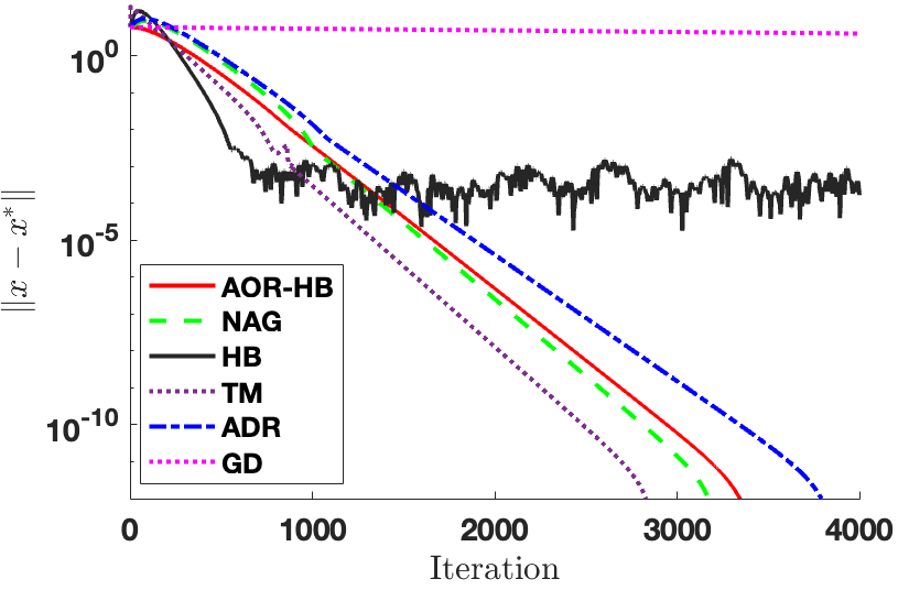
Figure 1: Simulation results using the objective (26) where $\mu=1,L=10^{4},d=100,p=5$ and $r=10^{-6}$.

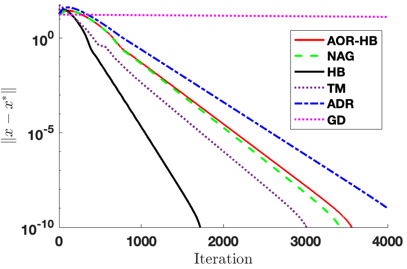
Figure 2: Simulation results for the logistic regression defined in (27) where $\lambda=0.1,d=1000,n=50$.

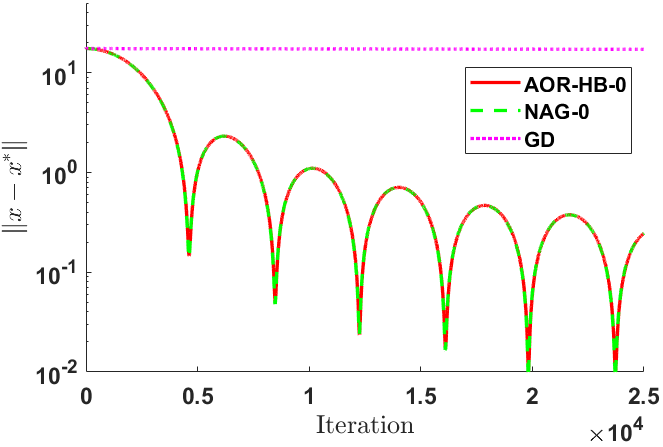
Figure 3: Simulation results for the logistic regression defined in (27) where $\lambda=1/d,d=1000,n=50$.

4.2 Policy evaluation problems with synthetic data

In this section, we compare AOR-HB-saddle (Algorithm 3) with the following algorithms: (i) AG-OG: accelerated gradient-optimistic gradient method with restarting regime  (Li et al., , 2023); (ii) APDG: accelerated primal-dual gradient method (Kovalev et al., , 2022); (iii) EG: a variant of extra-gradient method  (Mokhtari et al., , 2020).

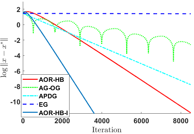
Figure 4: Simulation results for various methods to solve MSPBE: $\kappa_{g}=10^{4},\|\|B\|=10^{2}$.

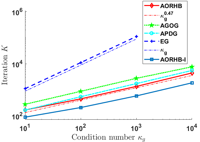
Figure 5: Iteration number required versus condition number for various algorithms.

We consider policy evaluation problems in reinforcement learning (Du et al., , 2017) when finding minimum of the mean squared projected Bellman error (MSPBE):

$$\arg\min_{u}\frac{1}{2}\|Bu-b\|_{C^{-1}}^{2}+\frac{1}{2}\|u\|^{2}.$$

The corresponding saddle point problem (see Appendix B.3) is

$$\min_{u\in\mathbb{R}^{m}}\max_{p\in\mathbb{R}^{n}}\frac{1}{2}\|u\|^{2}-\frac{1}{2}\|p\|_{C}^{2}-\langle b,p\rangle+\langle Bu,p\rangle.$$

The saddle point formulation saves the computation cost of inverting $C$. In this example, $\mu_{f}=L_{f}=1$, $\mu_{g}=\lambda_{\min}(C)$ and $L_{g}=\lambda_{\max}(C)$. We generate random matrices $B$ and $C$ such that $\mu_{g}=1$ and the condition number $\kappa_{g}=\|B\|^{2}$. We set $m=2500$ and $n=50$.

We plot the convergence of error versus number of iterations in Figure 5 for the case where $\kappa_{g}=10^{4}$. Different choices of condition numbers yield similar results, where our AOR-HB-saddle methods achieve much faster linear convergence than all other algorithms. AOR-HB-saddle has a single-loop structure and require fewer parameters to tune, which is favorable for implementation. In particular, AOR-HB-saddle-I is the semi-implicit scheme (25) with step size $\alpha=\sqrt{1/\kappa(g)}$. We use direct solver to compute $((1+\alpha)I+\frac{\alpha^{2}}{(1+\alpha)\mu_{f}\mu_{g}}BB^{\top})^{-1}$ since it is a small $50\times 50$ SPD matrix. As the step size is enlarged, AOR-HB-saddle-I converges fastest and is overall time-efficient especially when the coupling term $\|B\|^{2}/(\mu_{f}\mu_{g})$ is larger than $\sqrt{\kappa_{f}}$ and $\sqrt{\kappa_{g}}$.

In Figure 5, we plot the iteration number $K$ versus $\kappa_{g}$ such that $\frac{\|x_{K}-x^{*}\|}{\|x_{0}-x^{*}\|}\leq 10^{-6}$ for $x_{k}=(u_{k},p_{k})^{\top}$ generated by the algorithms. In this log-log scale plot, we can observe that the growth of iteration complexity is $\mathcal{O}(\sqrt{\kappa_{g}})$ for accelerated algorithms and $\mathcal{O}(\kappa_{g})$ for EG, which matches the convergence analysis. Among all accelerated algorithms we have tested, our AOR-HB-saddle method requires fewer iteration steps to achieve the desired accuracy and is simple to implement.

5 Concluding Remarks

In conclusion, we have introduced the Accelerated Over-Relaxation Heavy-Ball (AOR-HB) methods, a significant advancement of the accelerated first order optimization algorithms. Our method has been proven to exhibit global and accelerated convergence for not only smooth and strongly convex optimization problems but also a class of min-max problems with bilinear coupling. This breakthrough fills a theoretical gap in heavy-ball momentum methods and opens the door to developing accelerated methods with potential forays into non-convex optimization scenarios.

Although AOR-HB methods are accelerated first-order algorithms for convex and non-convex optimization, they still have some limitations. First, AOR-HB methods needs parameters $\mu$ and $L$. This is common for accelerated methods, but investigating adaptive strategies to reduce the parameters is an interesting future topic. Second, some rates in the theorems are not as tight as TM (Van Scoy et al., , 2017; Taylor and Drori, , 2023). A high-resolution ODE for obtaining the optimal rate is studied in Sun et al., (2020), which involves the Hessian. To understand and reveal the acceleration phenomenon of different ODE models is an interesting future topic. Third, expanding the applicability of the AOR-HB method to non-smooth, composite convex optimization, and/or weakly convex problems could significantly broaden its utility. Examining the algorithm’s behavior under stochastic conditions, such as noisy gradients or inherent stochasticity in objective functions, is crucial for understanding its robustness in practical applications in machine learning.

Appendix A Definitions and Standard Results

We review some foundational results from the convex analysis.

Recall that the Bregman divergence of $f$ is defined as

$$D_{f}(y,x):=f(y)-f(x)-\langle\nabla f(x),y-x\rangle,$$

which is in general non-symmetric, i.e., $D_{f}(y,x)\neq D_{f}(x,y)$. A symmetrized Bregman divergence is defined as

$$\langle\nabla f(x)-\nabla f(y),x-y\rangle=D_{f}(y,x)+D_{f}(x,y).$$

We have the following bounds on the Bregman divergence and the symmetrized Bregman divergence.

Lemma A.1 (Section 2.1 in Nesterov, (2018)).

Suppose $f:\mathbb{R}^{d}\rightarrow\mathbb{R}$ is $\mu$-strongly convex and $L$-smooth. For any $x,y\in\mathbb{R}^{d}$,

$$\frac{\mu}{2}\|x-y\|^{2} \leq D_{f}(y,x)\leq\frac{L}{2}\|x-y\|^{2},$$ (28a)

$$\frac{1}{2L}\|\nabla f(x)-\nabla f(y)\|^{2} \leq D_{f}(y,x)\leq\frac{1}{2\mu}\|\nabla f(x)-\nabla f(y)\|^{2},$$ (28b)

$$\mu\|x-y\|^{2} \leq\langle\nabla f(x)-\nabla f(y),x-y\rangle\leq L\|x-y\|^{2},$$ (28c)

$$\frac{1}{L}\|\nabla f(x)-\nabla f(y)\|^{2} \leq\langle\nabla f(x)-\nabla f(y),x-y\rangle\leq\frac{1}{\mu}\|\nabla f(x)-\nabla f(y)\|^{2}.$$ (28d)

The following three-point identity on the Bregman divergence will be used to replace the identity of squares.

Lemma A.2 (Bregman divergence identity (Chen and Teboulle, , 1993)).

If function $f:\mathbb{R}^{d}\rightarrow\mathbb{R}$ is differentiable, then for any $x,y,z\in\mathbb{R}^{d}$, it holds that

$$\langle\nabla f(y)-\nabla f(x),y-z\rangle=D_{f}(z,y)+D_{f}(y,x)-D_{f}(z,x).$$ (29)

Proof.

By definition,

$$D_{f}(z,y) =f(z)-f(y)-\langle\nabla f(y),z-y\rangle,$$

$$D_{f}(y,x) =f(y)-f(x)-\langle\nabla f(x),y-x\rangle,$$

$$D_{f}(z,x) =f(z)-f(x)-\langle\nabla f(x),z-x\rangle.$$

Direct calculation gives the identity. ∎

Appendix B Related Works

B.1 Extensions/Applications of heavy-ball methods

While the acceleration guarantee has not yet proved rigorously, applications of heavy-ball methods including extension to constrained and distributed optimization problems have confirmed its performance benefits over the standard gradient-based methods (Wang and Miller, , 2013; Ochs et al., , 2015; Ghadimi et al., , 2013; Diakonikolas and Jordan, , 2021).

Sutskever et al., (2013) showed that stochastic gradient descent with momentum improves the training of deep and recurrent neural networks. Also, using heavy-ball flow improves neural ODEs training and inference (Xia et al., , 2021). Recently, accelerated convergence of stochastic heavy-ball methods has been established in Pan et al., (2023); Bollapragada et al., (2022); Wang et al., (2021) but only for quadratic objectives. To get rid of the hyperparameters used in the heavy-ball methods, Saab Jr et al., (2022) proposed an adaptive heavy-ball that estimates the Polyak’s optimal hyper-parameters at each iteration.

B.2 First-order methods and dynamic system

One approach to better understand the mechanism of the iterative method is the continuous-time analysis: derive an ordinary differential equation (ODE) model which coincides with the iterative method taking step size close to zero. Starting from the accelerated first-order methods for unconstrained optimization, an important milestone in this direction is to understand the acceleration from the variational perspective (Su et al., , 2016; Wibisono et al., , 2016). While the iterative methods are first-order, the continuous-time dynamics proposed for accelerated methods are high-order or high-resolution ODEs (Shi et al., , 2022; Sun et al., , 2020; Muehlebach and Jordan, , 2019; Attouch et al., , 2000). With the continuous-time dynamic, novel accelerated methods are proposed by time discretization of the ODE model and usually the behaviour of the dynamic facilitates the convergence analysis of the iterative methods (Krichene et al., , 2015; Luo and Chen, , 2022; Aujol et al., , 2022; Wilson et al., , 2021; Siegel, , 2019).

Due to the appealing results, systematic framework to draw connection between the dynamic system and the accelerated iterative method gains lots of interest (Scieur et al., , 2017; Ushiyama et al., , 2024; Taylor et al., , 2018; Sanz Serna and Zygalakis, , 2021). In fact, the theory and methods developed for other problem classes often build upon the work done in unconstrained optimization (Diakonikolas and Orecchia, , 2019).

B.3 Applications of strongly-convex-strongly concave saddle point problems with bilinear coupling

A classical application is the regularized empirical risk minimization (ERM) with linear predictors, which is a classical supervised learning problem. Given a data matrix $B=[b_{1},b_{2},\cdots,b_{n}]^{\top}\in\mathbb{R}^{n\times m}$ where $b_{i}\in\mathbb{R}^{m}$ is the feature vector of the $i$-th data entry, the ERM problem aims to solve

$$\min_{u\in\mathbb{R}^{m}}g(Bu)+f(u),$$ (30)

where $g:\mathbb{R}^{n}\to\mathbb{R}$ is some strongly convex loss function, $f:\mathbb{R}^{m}\to\mathbb{R}$ is a strongly convex regularizer and $u\in\mathbb{R}^{m}$ is the linear predictor. Equivalently, we can solve the saddle point problem

$$\min_{u\in\mathbb{R}^{m}}\max_{p\in\mathbb{R}^{n}}\left\{p^{\top}Bu-g^{*}(p)+f(u)\right\}.$$ (31)

The saddle point formulation is favorable in many scenarios, for instance (Zhang and Xiao, , 2017; Du and Hu, , 2019; Lei et al., , 2017).

Another application is policy evaluation problems in reinforcement learning when finding minimum the mean squared projected Bellman error (Du et al., , 2017):

$$\arg\min_{u}\frac{1}{2}\|Bu-b\|_{C^{-1}}^{2}+\frac{1}{2}\|u\|^{2},$$

where $B,C$ are given matrices. The corresponding saddle point problem is

$$\min_{u\in\mathbb{R}^{m}}\max_{p\in\mathbb{R}^{n}}\frac{1}{2}\|u\|^{2}-\frac{1}{2}\|p\|_{C}^{2}-\langle b,p\rangle+\langle Bu,p\rangle.$$

The saddle point formulation saves the computation cost of inverting $C$.

Appendix C Proof of Theorem 1.1

Consider the Lyapunov function

$$\mathcal{E}({\bf x})=\mathcal{E}(x,y): =f(x)-f^{*}+\frac{\mu}{2}\|y-x^{*}\|^{2}=D_{f}(x,x^{*})+\frac{\mu}{2}\|y-x^{*}\|^{2},$$ (32)

and the modified Lyapunov function

$$\mathcal{E}^{\alpha}({\bf x})=\mathcal{E}^{\alpha}(x,y): =\mathcal{E}(x,y)+\alpha\langle\nabla f(x)-\nabla f(x^{*}),y-x^{*}\rangle$$ (33)

$$=D_{f}(x,x^{*})+\frac{\mu}{2}\|y-x^{*}\|^{2}+\alpha\langle\nabla f(x)-\nabla f(x^{*}),y-x^{*}\rangle.$$

The novelty of $\mathcal{E}^{\alpha}(x,y)$ is the inclusion of the cross term $\alpha\langle\nabla f(x)-\nabla f(x^{*}),y-x^{*}\rangle$.

We denote the right-hand side of the AGD flow (10) as

$$\mathcal{G}({\bf x})=\mathcal{G}(x,y):=\begin{pmatrix}y-x,\\ x-y-\frac{1}{\mu}\nabla f(x)\end{pmatrix}.$$

Lemma C.1 (Strong Lyapunov property (Luo and Chen, , 2022)).

$$-\langle\nabla\mathcal{E}(x,y),\mathcal{G}(x,y)\rangle\geq\mathcal{E}(x,y)+\frac{\mu}{2}\|x-y\|^{2},\quad\forall~{}x,y\in\mathbb{R}^{d}.$$ (34)

Proof.

By direct calculation and the $\mu$-convexity of $f$,

$$-\langle\nabla\mathcal{E}(x,y),\mathcal{G}(x,y)\rangle=\langle\nabla f(x),x-x^{*}\rangle-\mu\langle x-y,y-x^{*}\rangle$$

$$={} \langle\nabla f(x),x-x^{*}\rangle-\frac{\mu}{2}\left(\|x-x^{*}\|^{2}-\|x-y\|^{2}-\|y-x^{*}\|^{2}\right)$$

$$\geq{} f(x)-f(x^{*})+\frac{\mu}{2}\|y-x^{*}\|^{2}+\frac{\mu}{2}\|x-y\|^{2}={}\mathcal{E}(x,y)+\frac{\mu}{2}\|x-y\|^{2}.$$

∎

Lemma C.2.

Suppose $f:\mathbb{R}^{d}\rightarrow\mathbb{R}$ is $\mu$-strongly convex and $L$-smooth. Denote by $\rho=\mu/L$. For any two vectors ${\bf x}_{k},{\bf x}_{k+1}\in\mathbb{R}^{2d}$ and $\alpha>0$, we have the following inequality on the Bregman divergence of $\mathcal{E}$ defined by (32)

$$\left(1-\frac{\alpha}{\sqrt{\rho}}\right)D_{\mathcal{E}}({\bf x}_{k},{\bf x}_{k+1}) \leq{}D_{\mathcal{E}}({\bf x}_{k},{\bf x}_{k+1})\pm\alpha\langle y_{k+1}-y_{k},\nabla f(x_{k+1})-\nabla f(x_{k})\rangle$$

$$\leq\left(1+\frac{\alpha}{\sqrt{\rho}}\right)D_{\mathcal{E}}({\bf x}_{k},{\bf x}_{k+1}).$$

Proof.

Using the identity of squares (15) (for $y$) and Bregman divergence identity (29) (for $x$), we have the component form of

$$D_{\mathcal{E}}({\bf x}_{k},{\bf x}_{k+1})=D_{f}(x_{k},x_{k+1})+\frac{\mu}{2}\|y_{k}-y_{k+1}\|^{2}.$$

By Cauchy-Schwarz inequality and bound (28b) in Lemma A.1, we have

$$\alpha\left|\langle y_{k+1}-y_{k},\nabla f(x_{k+1})-\nabla f(x_{k})\rangle\right|\leq ~{}\frac{\alpha}{2\sqrt{\mu L}}\|\nabla f(x_{k})-\nabla f(x_{k+1})\|^{2}+\frac{\alpha\sqrt{L\mu}}{2}\|y_{k}-y_{k+1}\|^{2}$$

$$\leq ~{}\alpha\sqrt{\frac{L}{\mu}}D_{f}(x_{k},x_{k+1})+\frac{\alpha\sqrt{L\mu}}{2}\|y_{k}-y_{k+1}\|^{2}$$

$$= ~{}\alpha\sqrt{\frac{L}{\mu}}\left(D_{f}(x_{k},x_{k+1})+\frac{\mu}{2}\|y_{k}-y_{k+1}\|^{2}\right).$$

∎

By Lemma C.2 and $\mathcal{E}({\bf x})=D_{\mathcal{E}}({\bf x},{\bf x}^{*})$ where ${\bf x}^{*}:=(x^{*},x^{*})^{\top}$, it is straightforward to verify the following bounds for $\mathcal{E},~{}\mathcal{E}^{\alpha}$ as Lyapunov functions. Assume $0<\alpha\leq\sqrt{\rho}$ with $\rho=\frac{\mu}{L}$. Then

$$0\leq\mathcal{E}^{\alpha}({\bf x})\leq 2\mathcal{E}({\bf x}),\quad\forall~{}{\bf x}=(x,y)^{\top}\in\mathbb{R}^{2d}.$$ (35)

Now we are in the position to prove our first main result.

Proof of Theorem 1.1.

We write (14) as a correction of Implicit Euler discretization of (10):

$${\bf x}_{k+1}-{\bf x}_{k}=\alpha\mathcal{G}({\bf x}_{k+1})-\alpha\begin{pmatrix}y_{k+1}-y_{k}\\ \frac{1}{\mu}(\nabla f(x_{k+1})-\nabla f(x_{k}))\end{pmatrix}.$$ (36)

and substitude into the identity of $\mathcal{E}$

$$\mathcal{E}({\bf x}_{k+1})-\mathcal{E}({\bf x}_{k})=(\nabla\mathcal{E}({\bf x}_{k+1}),{\bf x}_{k+1}-{\bf x}_{k})-D_{\mathcal{E}}({\bf x}_{k},{\bf x}_{k+1})$$

$$=\alpha\langle\nabla\mathcal{E}({\bf x}_{k+1}),\mathcal{G}({\bf x}_{k+1})\rangle-\alpha\langle\nabla\mathcal{E}({\bf x}_{k+1}),\begin{pmatrix}y_{k+1}-y_{k}\\ \frac{1}{\mu}(\nabla f(x_{k+1})-\nabla f(x_{k}))\end{pmatrix}\rangle-D_{\mathcal{E}}({\bf x}_{k},{\bf x}_{k+1}).$$

We write out the component form of the middle term and split it as

$$\alpha\langle\nabla f(x_{k+1})-\nabla f(x^{*}),y_{k+1}-y_{k}\rangle+\alpha\langle y_{k+1}-x^{*},\nabla f(x_{k+1})-\nabla f(x_{k})\rangle$$

$$={} \alpha\langle\nabla f(x_{k+1})-\nabla f(x^{*}),y_{k+1}-x^{*}\rangle+\alpha\langle y_{k+1}-y_{k},\nabla f(x_{k+1})-\nabla f(x_{k})\rangle$$

$$-\alpha\langle y_{k}-x^{*},\nabla f(x_{k})-\nabla f(x^{*})\rangle.$$

Substitute back to (19) and rearrange terms, we obtain the following identity:

$$\mathcal{E}^{\alpha}({\bf x}_{k+1})-\mathcal{E}^{\alpha}({\bf x}_{k})= ~{}\alpha\langle\nabla\mathcal{E}({\bf x}_{k+1}),\mathcal{G}({\bf x}_{k+1})\rangle$$ (37)

$$-D_{\mathcal{E}}({\bf x}_{k},{\bf x}_{k+1})-\alpha\langle y_{k+1}-y_{k},\nabla f(x_{k+1})-\nabla f(x_{k})\rangle,$$

By Lemma C.2, we can drop the terms in the second line for $0\leq\alpha\leq\sqrt{\rho}$. Use the strong Lyapunov property (34) and bound (35), we have

$$\mathcal{E}^{\alpha}({\bf x}_{k+1})-\mathcal{E}^{\alpha}({\bf x}_{k})\leq-\alpha\mathcal{E}({\bf x}_{k+1})\leq-\frac{\alpha}{2}\mathcal{E}^{\alpha}({\bf x}_{k+1}),$$ (38)

which implies the global linear convergence of $\mathcal{E}^{\alpha}$:

$$\mathcal{E}^{\alpha}({\bf x}_{k+1})\leq\frac{1}{1+\alpha/2}\mathcal{E}^{\alpha}({\bf x}_{k})\leq\left(\frac{1}{1+\alpha/2}\right)^{k+1}\mathcal{E}^{\alpha}({\bf x}_{0}),\quad k\geq 0.$$

Moreover, (38) implies

$$\mathcal{E}({\bf x}_{k+1})\leq\frac{1}{\alpha}(\mathcal{E}^{\alpha}({\bf x}_{k})-\mathcal{E}^{\alpha}({\bf x}_{k+1}))\leq\frac{1}{\alpha}\mathcal{E}^{\alpha}({\bf x}_{k})\leq\frac{1}{\alpha}\left(\frac{1}{1+\alpha/2}\right)^{k}\mathcal{E}^{\alpha}({\bf x}_{0}),$$

which coincides with (5) with $C_{0}=\frac{1}{\alpha}\mathcal{E}^{\alpha}({\bf x}_{0})\geq 0$. ∎

Appendix D Equivalent formulation of AOR-HB-saddle

Algorithm 2 is equivalent to the following discretization of the HB-saddle flow (45):

$$\frac{u_{k+1}-u_{k}}{\alpha} =v_{k}-u_{k+1},$$ (39a)

$$\frac{p_{k+1}-p_{k}}{\alpha} =q_{k}-p_{k+1},$$ (39b)

$$\frac{v_{k+1}-v_{k}}{\alpha} =u_{k+1}-v_{k+1}-\frac{1}{\mu_{f}}\left(2\nabla f(u_{k+1})-\nabla f(u_{k})+B^{\top}q_{k}\right),$$ (39c)

$$\frac{q_{k+1}-q_{k}}{\alpha} =p_{k+1}-q_{k+1}-\frac{1}{\mu_{g}}\left(2\nabla g(p_{k+1})-\nabla g(p_{k})-B(2v_{k+1}-v_{k})\right).$$ (39d)

The discretization is a mixture of implicit Euler and explicit Euler with time step size $\alpha$. For both the gradient terms and $Bv$ term, we use the AOR technique, i.e., $\nabla f(u)\approx 2\nabla f(u_{k+1})-\nabla f(u_{k})$, $\nabla g(p)\approx 2\nabla g(p_{k+1})-\nabla g(p_{k})$ and $Bv\approx B(2v_{k+1}-v_{k})$. Algorithm 3 is implementation-friendly while (39) is convenient for deriving convergence analysis.

Appendix E Proofs of Section 3

E.1 A class of monotone operator equations

In fact, we can extend HB flow to a broad class of monotone operator equation $\mathcal{A}(x)=0$ with

$$\mathcal{A}(x)=\nabla F(x)+\mathcal{N}x,$$ (40)

where $F$ is a strongly convex function and $L_{F}$ smooth, and $\mathcal{N}$ is a linear and skew-symmetric operator, i.e., $\mathcal{N}^{\top}=-\mathcal{N}$. Then $\mathcal{A}$ is Lipschitz continuous with constant $L_{\mathcal{A}}\leq L_{F}+\|\mathcal{N}\|$. Therefore $\mathcal{A}$ is monotone and Lipschitz continuous which is also known as inverse-strongly monotonicity (Browder and Petryshyn, , 1967; Liu and Nashed, , 1998) or co-coercitivity (Zhu and Marcotte, , 1996). Consequently equation $\mathcal{A}(x)=0$ has a unique solution $x^{*}$ (Rockafellar, , 1976).

As a special case, we recover strongly-convex-strongly-concave saddle point problems with bilinear coupling when $x:=(u,p)^{\top}$, $F(x):=f(u)+g(p)$ and $\mathcal{N}:=\begin{pmatrix}0&\;B^{\top}\\ -B&\;0\end{pmatrix}.$

We introduce an accelerated gradient flow

$$\left\{\begin{aligned} x^{\prime}&=y-x,\\ y^{\prime}&=x-y-\mu^{-1}(\nabla F(x)+\mathcal{N}y).\end{aligned}\right.$$ (41)

Comparing with the accelerated gradient flow (10) for convex optimization, the difference is the gradient and skew-symmetric splitting $\mathcal{A}(x)\rightarrow\nabla F(x)+\mathcal{N}y$.

Denote the vector field on the right hand side of (41) by $\mathcal{G}(x,y)$. Then $\mathcal{G}(x^{*},x^{*})=0$ and thus $(x^{*},x^{*})$ is an equilibrium point of (41).

We first show $(x^{*},x^{*})$ is exponentially stable. Consider the Lyapunov function:

$$\mathcal{E}(x,y)=D_{F}(x,x^{*})+\frac{\mu}{2}\|y-x^{*}\|^{2}.$$ (42)

For $\mu$-strongly convex $F$, function $D_{F}(\cdot,x^{*})\in\mathcal{S}_{\mu}$. Then $\mathcal{E}(x,y)\geq 0$ and $\mathcal{E}(x,y)=0$ iff $x=y=x^{*}$.

We then verify the strong Lyapunov property. The proof is similar to that of Lemma C.1.

Theorem E.1 (Strong Lyapunov Property).

Assume function $F$ is $\mu$-strongly convex. Then for the Lyapunov function (42) and the accelerated gradient flow vector field $\mathcal{G}$ asoociated to (41), the following strong Lyapunov property holds

$$-\nabla\mathcal{E}(x,y)\cdot\mathcal{G}(x,y)\geq\mathcal{E}(x,y)+\frac{\mu}{2}\|y-x\|^{2},\quad\forall~{}x,y\in\mathcal{V}.$$ (43)

Proof.

First of all, as $\mathcal{G}(x^{*},x^{*})=0$,

$$-\langle\nabla\mathcal{E}(x,y),\mathcal{G}(x,y)\rangle=-\langle\nabla\mathcal{E}(x,y),\mathcal{G}(x,y)-\mathcal{G}(x^{*},x^{*})\rangle.$$

Direct computation gives

$$-\langle\nabla\mathcal{E}(x,y),\mathcal{G}(x,y)\rangle= ~{}\langle\nabla D_{F}(x,x^{*}),x-x^{*}-(y-x^{*})\rangle-\mu\langle y-x^{*},x-x^{*}\rangle$$

$$+\mu\|y-x^{*}\|^{2} +\langle\nabla F(x)-\nabla F(x^{*}),y-x^{*}\rangle+\langle y-x^{*},\mathcal{N}(y-x^{*})\rangle$$

$$=~{}\langle\nabla F(x) -\nabla F(x^{*}),x-x^{*}\rangle+\mu\|y-x^{*}\|^{2}-\mu\langle y-x^{*},x-x^{*}\rangle,$$

where we have used $\nabla D_{F}(x,x^{*})=\nabla F(x)-\nabla F(x^{*})$ and $\langle y-x^{*},\mathcal{N}(y-x^{*})\rangle=0$ since $\mathcal{N}$ is skew-symmetric. We expand the last two term using the identity of squares: (15)

$$\frac{1}{2}\|y-x^{*}\|^{2}-\langle y-x^{*},x-x^{*}\rangle=\frac{1}{2}\|y-x\|^{2}-\frac{1}{2}\|x-x^{*}\|^{2}.$$

Using the bound (28a), we get

$$\langle\nabla F(x)-\nabla F(x^{*}),x-x^{*}\rangle=D_{F}(x,x^{*})+D_{F}(x^{*},x)\geq D_{F}(x,x^{*})+\frac{\mu}{2}\|x-x^{*}\|^{2}$$

and obtain (43). ∎

The calculation is more clear when $\nabla F(x)=Ax$ is linear with $A=\nabla^{2}F\geq\mu I$. We denote by ${\bf x}=(x,y)^{\top}$ and $\mathcal{E}({\bf x})=\frac{1}{2}\|{\bf x}-{\bf x}^{*}\|_{\mathcal{D}}^{2}$ with $\mathcal{D}=\begin{pmatrix}A&0\\ 0&\mu I\end{pmatrix}$. Then $-\langle\nabla\mathcal{E}(x,y),\mathcal{G}(x,y)-\mathcal{G}(x^{*},x^{*})\rangle$ is a quadratic form $({\bf x}-{\bf x}^{*})^{\top}\mathcal{M}({\bf x}-{\bf x}^{*})$. We calculate the matrix $\mathcal{M}$ as

$$\begin{pmatrix}A&0\\ 0&\mu I\end{pmatrix}\begin{pmatrix}I&-I\\ -I+\mu^{-1}A&\quad I+\mu^{-1}\mathcal{N}\end{pmatrix}=\begin{pmatrix}A&-A\\ -\mu I+A&\;\mu I+\mathcal{N}\end{pmatrix}.$$

As $v^{\top}Mv=v^{\top}\operatorname{sym}(M)v$ where $\operatorname{sym}(\cdot)$ is the symmetric part of a matrix, direct computation gives

$$\operatorname{sym}\begin{pmatrix}A&-A\\ -\mu I+A&\;\mu I+\mathcal{N}\end{pmatrix} =\begin{pmatrix}A&-\mu I/2\\ -\mu I/2&\mu I\end{pmatrix}$$

$$\geq\begin{pmatrix}A/2&0\\ 0&\;\mu I/2\end{pmatrix}+\frac{1}{2}\begin{pmatrix}\mu I&-\mu I\\ -\mu I&\;\mu I\end{pmatrix},$$

where in the last step we use the convexity $A\geq\mu I$. Then (43) follows.

E.2 Exponential stability of HB-saddle flow

Return to the saddle point problems, we let ${\bf x}=(x,y)^{\top}$ with $x=(u,p)^{\top},y=(v,q)^{\top}\in\mathbb{R}^{m}\times\mathbb{R}^{n}$ and denote by

$$F(x):=f(u)+g(p),\ \mathcal{N}:=\begin{pmatrix}0&\;B^{\top}\\ -B&\;0\end{pmatrix},\ \mathcal{D}_{\mu}:=\begin{pmatrix}\mu_{f}&0\\ 0&\mu_{g}\end{pmatrix}.$$

Consider the Lyapunov function

$$\mathcal{E}({\bf x})=\mathcal{E}(u,v,p,q) :=D_{F}(x,x^{*})+\frac{1}{2}\|y-x^{*}\|_{\mathcal{D}_{\mu}}^{2}$$ (44)

$$=D_{f}(u,u^{*})+D_{g}(p,p^{*})+\frac{\mu_{f}}{2}\|u-u^{*}\|^{2}+\frac{\mu_{g}}{2}\|p-p^{*}\|^{2},$$

As $f,g$ are strongly convex, $\mathcal{E}({\bf x})\geq 0$ and $\mathcal{E}({\bf x})=0$ iff $u=v=u^{*}$ and $p=q=p^{*}$.

Recall that the HB-saddle flow is

$$u^{\prime} =v-u,$$ (45)

$$p^{\prime} =q-p,$$

$$v^{\prime} =u-v-\frac{1}{\mu_{f}}(\nabla f(u)+B^{\top}q),$$

$$q^{\prime} =p-q-\frac{1}{\mu_{g}}(\nabla g(p)-Bv).$$

Denoted the vector field on the right hand side of (45) by $\mathcal{G}(u,v,p,q)$, as a special case of Theorem E.1, we obtain the following strong Lyapunov property.

Theorem E.2 (Strong Lyapunov property for HB-saddle flow).

Suppose $f$ is $\mu_{f}$-strongly convex $g$ is $\mu_{g}$-strongly convex. The following strong Lyapunov property holds for all $u,v\in\mathbb{R}^{m},p,q\in\mathbb{R}^{n}$.

$$-\langle\nabla\mathcal{E}(u,v,p,q),\mathcal{G}(u,v,p,q)\rangle\geq\mathcal{E}(u,v,p,q)+\frac{\mu_{f}}{2}\|v-u\|^{2}+\frac{\mu_{g}}{2}\|q-p\|^{2}.$$ (46)

Consequently, for solutions $(u(t),v(t),p(t),q(t))$ of the HB-saddle flow (24), we have the exponential stability:

$$D_{f}(u,u^{*})+D_{g}(p,p^{*})+\frac{\mu_{f}}{2}\|v-u^{*}\|^{2}+\frac{\mu_{g}}{2}\|q-p^{*}\|^{2}\leq e^{-t}\mathcal{E}(u(0),v(0),p(0),q(0)),~{}\quad t>0.$$

E.3 Proof of Theorem 1.2

Consider the modified Lyapunov function

$$\mathcal{E}^{\alpha}({\bf x}) :=\mathcal{E}({\bf x})+\alpha\langle\nabla F(x)-\nabla F(x^{*}),y-x^{*}\rangle-\alpha\|y-y^{*}\|^{2}_{\mathcal{B}^{\operatorname{sym}}},$$ (47)

where $\mathcal{E}({\bf x})$ is defined as (44) and $\mathcal{B}^{\operatorname{sym}}=\begin{pmatrix}0&B^{\top}\\ B&0\end{pmatrix}$. Due to the bilinear coupling, additional cross term $\alpha\|y-y^{*}\|^{2}_{\mathcal{B}^{\operatorname{sym}}}=2\alpha(B(v-v^{*}),q-q^{*})$ is included in $\mathcal{E}^{\alpha}$.

We shall split $\frac{1}{2}\|y-x^{*}\|_{\mathcal{D}_{\mu}}^{2}$ to $\frac{\beta}{2}\|y-x^{*}\|_{\mathcal{D}_{\mu}}^{2}+\frac{1-\beta}{2}\|y-x^{*}\|_{\mathcal{D}_{\mu}}^{2}$ to bound the two cross terms. The cross term $\alpha\langle\nabla F(x)-\nabla F(x^{*}),y-x^{*}\rangle$ can be bounded using the vector form of Lemma C.2. Next we focus on the $\alpha\|y-y^{*}\|^{2}_{\mathcal{B}^{\operatorname{sym}}}$.

Lemma E.1.

Denoted by $\mathcal{D}_{\mu}=\begin{pmatrix}\mu_{f}I&\;0\\ 0&\;\mu_{g}I\end{pmatrix}$ with $\mu_{f},\mu_{g}>0$ and $\mathcal{B}^{\operatorname{sym}}=\begin{pmatrix}0&B^{\top}\\ B&0\end{pmatrix}$. For any $\alpha,c>0$, we have

$$\left(1-\frac{\alpha\|B\|}{c\sqrt{\mu_{f}\mu_{g}}}\right)c\mathcal{D}\leq c\mathcal{D}_{\mu}\pm\alpha\mathcal{B}^{\operatorname{sym}}\leq\left(1+\frac{\alpha\|B\|}{c\sqrt{\mu_{f}\mu_{g}}}\right)c\mathcal{D}_{\mu}.$$ (48)

Proof.

We first calculate the eigenvalues of $\mathcal{D}_{\mu}^{-1}\mathcal{B}^{\operatorname{sym}}$. By choosing the SVD basis of $B=U\Sigma V$, its eigenvalue is given by the $2\times 2$ matrix $\begin{pmatrix}0&\mu_{f}^{-1}\sigma(B)\\ \mu_{g}^{-1}\sigma(B)&0\end{pmatrix}$, where $\sigma(B)$ is a singular value of $B$. So $\lambda(\mathcal{D}_{\mu}^{-1}\mathcal{B}^{\operatorname{sym}})=\pm\frac{\sigma(B)}{\sqrt{\mu_{f}\mu_{g}}}$ and consequently

$$-\frac{\|B\|}{\sqrt{\mu_{f}\mu_{g}}}\leq\lambda_{\min}(\mathcal{D}_{\mu}^{-1}\mathcal{B}^{\operatorname{sym}})\leq\lambda_{\max}(\mathcal{D}_{\mu}^{-1}\mathcal{B}^{\operatorname{sym}})\leq\frac{\|B\|}{\sqrt{\mu_{f}\mu_{g}}}.$$ (49)

Then write $c\mathcal{D}_{\mu}\pm\alpha\mathcal{B}^{\operatorname{sym}}=c\mathcal{D}_{\mu}(I\pm\frac{\alpha}{c}\mathcal{D}_{\mu}^{-1}\mathcal{B}^{\operatorname{sym}})$ and apply the bound (49) to get the desired result. ∎

Lemma E.2.

Suppose $f:\mathbb{R}^{m}\rightarrow\mathbb{R}$ is $\mu_{f}$-strongly convex and $L_{f}$-smooth, $g:\mathbb{R}^{n}\rightarrow\mathbb{R}$ is $\mu_{g}$-strongly convex and $L_{g}$-smooth. Let $F({\bf x})=f(u)+g(p)$. Denoted by

$$\sqrt{\rho}=(\sqrt{2}-1)\min\left\{\sqrt{\frac{\mu_{f}}{L_{f}}},\sqrt{\frac{\mu_{g}}{L_{g}}},\frac{\sqrt{\mu_{f}\mu_{g}}}{\|B\|}\right\}.$$

Then for any $\alpha>0$ and $\mathcal{E}$ defined by (44) and any two vectors ${\bf x}_{k},{\bf x}_{k+1}\in\mathbb{R}^{2(m+n)}$

$$\left(1-\frac{\alpha}{\sqrt{\rho}}\right)D_{\mathcal{E}}({\bf x}_{k},{\bf x}_{k+1})$$ (50)

$$\leq{} D_{\mathcal{E}}({\bf x}_{k},{\bf x}_{k+1})\pm\alpha\langle y_{k+1}-y_{k},\nabla F(x_{k+1})-\nabla F(x_{k})\rangle\pm\alpha\|y_{k}-y_{k+1}\|^{2}_{\mathcal{B}^{\operatorname{sym}}},$$

$$\leq{} \left(1+\frac{\alpha}{\sqrt{\rho}}\right)D_{\mathcal{E}}({\bf x}_{k},{\bf x}_{k+1}).$$

In particular, for $\alpha\leq\sqrt{\rho}$, we have the bound

$$0\leq\mathcal{E}^{\alpha}({\bf x})\leq 2\mathcal{E}({\bf x})\quad{\bf x}\in\mathbb{R}^{2d}.$$ (51)

Proof.

For any $\beta\in(0,1)$, using the vector form of Lemma C.2, we have bound

$$\left(1-\frac{\alpha}{\sqrt{\rho_{F}}}\right)\left(D_{F}(x_{k},x_{k+1})+\frac{\beta}{2}\|y_{k}-y_{k+1}\|_{\mathcal{D}_{\mu}}^{2}\right)$$ (52)

$$\leq{} D_{F}(x_{k},x_{k+1})+\frac{\beta}{2}\|y_{k}-y_{k+1}\|_{\mathcal{D}_{\mu}}^{2}\pm\alpha\langle y_{k+1}-y_{k},\nabla F(x_{k+1})-\nabla F(x_{k})\rangle$$

$$\leq{} \left(1+\frac{\alpha}{\sqrt{\rho_{F}}}\right)\left(D_{F}(x_{k},x_{k+1})+\frac{\beta}{2}\|y_{k}-y_{k+1}\|_{\mathcal{D}_{\mu}}^{2}\right)$$

with $\rho_{F}=\beta\min\left\{\frac{\mu_{f}}{L_{f}},\frac{\mu_{g}}{L_{g}}\right\}$.

Use Lemma E.1, we have the bound

$$\left(1-\frac{2\alpha\|B\|}{(1-\beta)\sqrt{\mu_{f}\mu_{g}}}\right)\frac{1-\beta}{2}\|y_{k}-y_{k+1}\|_{\mathcal{D}_{\mu}}^{2} \leq\frac{1-\beta}{2}\|y_{k}-y_{k+1}\|_{\mathcal{D}_{\mu}}^{2}\pm\alpha\|y_{k}-y_{k+1}\|^{2}_{\mathcal{B}^{\operatorname{sym}}}$$ (53)

$$\leq\left(1+\frac{2\alpha\|B\|}{(1-\beta)\sqrt{\mu_{f}\mu_{g}}}\right)\frac{1-\beta}{2}\|y_{k}-y_{k+1}\|_{\mathcal{D}_{\mu}}^{2}.$$

Choose $\beta\in(0,1)$ s.t. $\sqrt{\beta}=\frac{1-\beta}{2}$, i.e., $\beta=3-2\sqrt{2}$ and $\sqrt{\beta}=\sqrt{2}-1$. Adding (52) and (53) implies (50).

Apply (50) with ${\bf x}_{k}={\bf x}$ and ${\bf x}_{k+1}={\bf x}^{*}$ to get (51). ∎

Now we are ready to prove the theorem.

Proof of Theorem 1.2.

We write (39) as a correction of the implicit Euler method

$${\bf x}_{k+1}-{\bf x}_{k}=\alpha\mathcal{G}({\bf x}_{k+1})-\alpha\begin{pmatrix}0&I\\ \mathcal{D}_{\mu}^{-1}\nabla F&0\end{pmatrix}({\bf x}_{k+1}-{\bf x}_{k})-\alpha\begin{pmatrix}0\\ \mathcal{D}_{\mu}^{-1}\mathcal{B}^{\operatorname{sym}}(y_{k+1}-y_{k})\end{pmatrix}.$$ (54)

Use the definition of Bregman divergence, we have the identity for the difference of the Lyapunov function $\mathcal{E}$ at consecutive steps:

$$\mathcal{E}({\bf x}_{k+1})-\mathcal{E}({\bf x}_{k})=(\nabla\mathcal{E}({\bf x}_{k+1}),{\bf x}_{k+1}-{\bf x}_{k})-D_{\mathcal{E}}({\bf x}_{k},{\bf x}_{k+1})$$

Substitute (54) and expand the cross term:

$$\langle\nabla\mathcal{E}({\bf x}_{k+1}), {\bf x}_{k+1}-{\bf x}_{k}\rangle={}\alpha\langle\nabla\mathcal{E}({\bf x}_{k+1}),\mathcal{G}({\bf x}_{k+1})\rangle$$ (55)

$$- \alpha\langle\nabla F(x_{k+1})-\nabla F(x^{*}),y_{k+1}-y_{k}\rangle-\alpha\langle y_{k+1}-x^{*},\nabla F(x_{k+1})-\nabla F(x_{k})\rangle$$

$$- \alpha\langle y_{k+1}-y^{*},y_{k+1}-y_{k}\rangle_{\mathcal{B}^{\operatorname{sym}}}$$

We split the gradient term as

$$\alpha\langle\nabla F(x_{k+1})-\nabla F(x^{*}),y_{k+1}-y_{k}\rangle+\alpha\langle y_{k+1}-x^{*},\nabla F(x_{k+1})-\nabla F(x_{k})\rangle$$

$$={} \alpha\langle\nabla F(x_{k+1})-\nabla F(x^{*}),y_{k+1}-x^{*}\rangle+\alpha\langle y_{k+1}-y_{k},\nabla F(x_{k+1})-\nabla F(x_{k})\rangle$$

$$-\alpha\langle y_{k}-x^{*},\nabla F(x_{k})-\nabla F(x^{*})\rangle.$$

We can use identity of squares (15) to expand

$$\langle y_{k+1}-y^{*},y_{k+1}-y_{k}\rangle_{\mathcal{B}^{\operatorname{sym}}}=\frac{1}{2}\left(\|y_{k+1}-y^{*}\|_{\mathcal{B}^{\operatorname{sym}}}^{2}+\|y_{k+1}-y_{k}\|_{\mathcal{B}^{\operatorname{sym}}}^{2}-\|y_{k}-y^{*}\|_{\mathcal{B}^{\operatorname{sym}}}^{2}\right).$$

Substitute back to (19) and rearrange terms, we obtain the following identity:

$$\mathcal{E}^{\alpha}({\bf x}_{k+1})-\mathcal{E}^{\alpha}({\bf x}_{k})=~{}\alpha\langle\nabla\mathcal{E}({\bf x}_{k+1}),\mathcal{G}({\bf x}_{k+1})\rangle$$ (56)

$$-D_{\mathcal{E}}({\bf x}_{k},{\bf x}_{k+1})+\alpha\langle y_{k+1}-y_{k},\nabla F(x_{k+1})-\nabla F(x_{k})\rangle-\alpha\|y_{k}-y_{k+1}\|^{2}_{\mathcal{B}^{\operatorname{sym}}},$$

which holds for arbitrary step size $\alpha$.

Now take $\alpha\leq\sqrt{\rho}$. The last term in (56) is non-positive. Use the strong Lyapunov property, and the bound $\mathcal{E}^{\alpha}({\bf x})\leq 2\mathcal{E}({\bf x})$ to get

$$\mathcal{E}^{\alpha}({\bf x}_{k+1})-\mathcal{E}^{\alpha}({\bf x}_{k})\leq-\alpha\mathcal{E}({\bf x}_{k+1})\leq-\frac{\alpha}{2}\mathcal{E}^{\alpha}({\bf x}_{k+1}),$$ (57)

which implies the global linear convergence:

$$\mathcal{E}^{\alpha}({\bf x}_{k+1})\leq\frac{1}{1+\alpha/2}\mathcal{E}^{\alpha}({\bf x}_{k})\leq\left(\frac{1}{1+\alpha/2}\right)^{k+1}\mathcal{E}^{\alpha}({\bf x}_{0}),\quad k\geq 0.$$

Moreover, (57) implies

$$\mathcal{E}({\bf x}_{k+1})\leq\frac{1}{\alpha}(\mathcal{E}^{\alpha}({\bf x}_{k})-\mathcal{E}^{\alpha}({\bf x}_{k+1}))\leq\frac{1}{\alpha}\mathcal{E}^{\alpha}({\bf x}_{k})\leq\frac{1}{\alpha}\left(\frac{1}{1+\alpha/2}\right)^{k}\mathcal{E}^{\alpha}({\bf x}_{0}),$$

which coincides with (5) with $C_{0}=\frac{1}{\alpha}\mathcal{E}^{\alpha}({\bf x}_{0})\geq 0$. ∎

References

• Attouch et al., (2000) Attouch, H., Goudou, X., and Redont, P. (2000). The heavy ball with friction method, i. the continuous dynamical system: global exploration of the local minima of a real-valued function by asymptotic analysis of a dissipative dynamical system. Communications in Contemporary Mathematics, 2(01):1–34.
• Aujol et al., (2022) Aujol, J.-F., Dossal, C., and Rondepierre, A. (2022). Convergence rates of the heavy ball method for quasi-strongly convex optimization. SIAM Journal on Optimization, 32(3):1817–1842.
• Bollapragada et al., (2022) Bollapragada, R., Chen, T., and Ward, R. (2022). On the fast convergence of minibatch heavy ball momentum. arXiv preprint arXiv:2206.07553.
• Bottou et al., (2018) Bottou, L., Curtis, F. E., and Nocedal, J. (2018). Optimization methods for large-scale machine learning. SIAM review, 60(2):223–311.
• Browder and Petryshyn, (1967) Browder, F. E. and Petryshyn, W. V. (1967). Construction of fixed points of nonlinear mappings in Hilbert space. Journal of Mathematical Analysis and Applications, 20(2):197–228.
• Bubeck et al., (2015) Bubeck, S., Lee, Y. T., and Singh, M. (2015). A geometric alternative to Nesterov’s accelerated gradient descent. arXiv preprint arXiv:1506.08187.
• Chen and Teboulle, (1993) Chen, G. and Teboulle, M. (1993). Convergence analysis of a proximal-like minimization algorithm using Bregman functions. SIAM Journal on Optimization, 3(3):538–543.
• Chen and Luo, (2021) Chen, L. and Luo, H. (2021). A unified convergence analysis of first order convex optimization methods via strong Lyapunov functions. arXiv preprint arXiv:2108.00132, 4(9):10.
• Cyrus et al., (2018) Cyrus, S., Hu, B., Van Scoy, B., and Lessard, L. (2018). A robust accelerated optimization algorithm for strongly convex functions. In 2018 Annual American Control Conference (ACC), pages 1376–1381. IEEE.
• Diakonikolas and Jordan, (2021) Diakonikolas, J. and Jordan, M. I. (2021). Generalized momentum-based methods: A Hamiltonian perspective. SIAM Journal on Optimization, 31(1):915–944.
• Diakonikolas and Orecchia, (2019) Diakonikolas, J. and Orecchia, L. (2019). The approximate duality gap technique: A unified theory of first-order methods. SIAM Journal on Optimization, 29(1):660–689.
• Drusvyatskiy et al., (2018) Drusvyatskiy, D., Fazel, M., and Roy, S. (2018). An optimal first order method based on optimal quadratic averaging. SIAM Journal on Optimization, 28(1):251–271.
• Du et al., (2017) Du, S. S., Chen, J., Li, L., Xiao, L., and Zhou, D. (2017). Stochastic variance reduction methods for policy evaluation. In International Conference on Machine Learning, pages 1049–1058. PMLR.
• Du and Hu, (2019) Du, S. S. and Hu, W. (2019). Linear convergence of the primal-dual gradient method for convex-concave saddle point problems without strong convexity. In The 22nd International Conference on Artificial Intelligence and Statistics, pages 196–205. PMLR.
• Ghadimi et al., (2015) Ghadimi, E., Feyzmahdavian, H. R., and Johansson, M. (2015). Global convergence of the heavy-ball method for convex optimization. In 2015 European control conference (ECC), pages 310–315. IEEE.
• Ghadimi et al., (2013) Ghadimi, E., Shames, I., and Johansson, M. (2013). Multi-step gradient methods for networked optimization. IEEE Transactions on Signal Processing, 61(21):5417–5429.
• Goujaud et al., (2023) Goujaud, B., Taylor, A., and Dieuleveut, A. (2023). Provable non-accelerations of the heavy-ball method. arXiv preprint arXiv:2307.11291.
• Hadjidimos, (1978) Hadjidimos, A. (1978). Accelerated overrelaxation method. Mathematics of Computation, 32(141):149–157.
• Jin et al., (2022) Jin, Y., Sidford, A., and Tian, K. (2022). Sharper rates for separable minimax and finite sum optimization via primal-dual extragradient methods. In Conference on Learning Theory, pages 4362–4415. PMLR.
• Kovalev et al., (2022) Kovalev, D., Gasnikov, A., and Richtárik, P. (2022). Accelerated primal-dual gradient method for smooth and convex-concave saddle-point problems with bilinear coupling. Advances in Neural Information Processing Systems, 35:21725–21737.
• Krichene et al., (2015) Krichene, W., Bayen, A., and Bartlett, P. L. (2015). Accelerated mirror descent in continuous and discrete time. Advances in neural information processing systems, 28.
• Lei et al., (2017) Lei, Q., Yen, I. E.-H., Wu, C.-y., Dhillon, I. S., and Ravikumar, P. (2017). Doubly greedy primal-dual coordinate descent for sparse empirical risk minimization. In International Conference on Machine Learning, pages 2034–2042. PMLR.
• Lessard et al., (2016) Lessard, L., Recht, B., and Packard, A. (2016). Analysis and design of optimization algorithms via integral quadratic constraints. SIAM Journal on Optimization, 26(1):57–95.
• Li et al., (2023) Li, C. J., Yuan, H., Gidel, G., Gu, Q., and Jordan, M. (2023). Nesterov meets optimism: rate-optimal separable minimax optimization. In International Conference on Machine Learning, pages 20351–20383. PMLR.
• Lin et al., (2015) Lin, H., Mairal, J., and Harchaoui, Z. (2015). A universal catalyst for first-order optimization. Advances in neural information processing systems, 28.
• Liu and Nashed, (1998) Liu, F. and Nashed, M. Z. (1998). Regularization of nonlinear ill-posed variational inequalities and convergence rates. Set-Valued Analysis, 6(4):313–344.
• Luo and Chen, (2022) Luo, H. and Chen, L. (2022). From differential equation solvers to accelerated first-order methods for convex optimization. Mathematical Programming, 195(1):735–781.
• Metelev et al., (2024) Metelev, D., Rogozin, A., Gasnikov, A., and Kovalev, D. (2024). Decentralized saddle-point problems with different constants of strong convexity and strong concavity. Computational Management Science, 21(1):5.
• Mokhtari et al., (2020) Mokhtari, A., Ozdaglar, A., and Pattathil, S. (2020). A unified analysis of extra-gradient and optimistic gradient methods for saddle point problems: Proximal point approach. In International Conference on Artificial Intelligence and Statistics, pages 1497–1507. PMLR.
• Muehlebach and Jordan, (2019) Muehlebach, M. and Jordan, M. (2019). A dynamical systems perspective on nesterov acceleration. In International Conference on Machine Learning, pages 4656–4662. PMLR.
• Nesterov, (1983) Nesterov, Y. (1983). A method of solving a convex programming problem with convergence rate $O(1/k^{2})$. Doklady Akademii Nauk SSSR, 269(3):543.
• Nesterov, (2013) Nesterov, Y. (2013). Introductory lectures on convex optimization: A basic course, volume 87. Springer Science & Business Media.
• Nesterov, (2018) Nesterov, Y. (2018). Lectures on convex optimization, volume 137. Springer.
• Ochs et al., (2015) Ochs, P., Brox, T., and Pock, T. (2015). iPiasco: inertial proximal algorithm for strongly convex optimization. Journal of Mathematical Imaging and Vision, 53:171–181.
• Pan et al., (2023) Pan, R., Liu, Y., Wang, X., and Zhang, T. (2023). Accelerated convergence of stochastic heavy ball method under anisotropic gradient noise. arXiv preprint arXiv:2312.14567.
• Polyak, (1964) Polyak, B. T. (1964). Some methods of speeding up the convergence of iteration methods. Ussr computational mathematics and mathematical physics, 4(5):1–17.
• Rockafellar, (1976) Rockafellar, R. T. (1976). Monotone operators and the proximal point algorithm. SIAM journal on control and optimization, 14(5):877–898.
• Saab Jr et al., (2022) Saab Jr, S., Phoha, S., Zhu, M., and Ray, A. (2022). An adaptive polyak heavy-ball method. Machine Learning, 111(9):3245–3277.
• Sanz Serna and Zygalakis, (2021) Sanz Serna, J. M. and Zygalakis, K. C. (2021). The connections between Lyapunov functions for some optimization algorithms and differential equations. SIAM Journal on Numerical Analysis, 59(3):1542–1565.
• Scieur et al., (2017) Scieur, D., Roulet, V., Bach, F., and d’Aspremont, A. (2017). Integration methods and optimization algorithms. Advances in Neural Information Processing Systems, 30.
• Shi et al., (2022) Shi, B., Du, S. S., Jordan, M. I., and Su, W. J. (2022). Understanding the acceleration phenomenon via high-resolution differential equations. Mathematical Programming, pages 1–70.
• Siegel, (2019) Siegel, J. W. (2019). Accelerated first-order methods: Differential equations and Lyapunov functions. arXiv preprint arXiv:1903.05671.
• Su et al., (2016) Su, W., Boyd, S., and Candes, E. J. (2016). A differential equation for modeling Nesterov’s accelerated gradient method: Theory and insights. Journal of Machine Learning Research, 17(153):1–43.
• Sun et al., (2020) Sun, B., George, J., and Kia, S. (2020). High-resolution modeling of the fastest first-order optimization method for strongly convex functions. In 2020 59th IEEE Conference on Decision and Control (CDC), pages 4237–4242. IEEE.
• Sun et al., (2019) Sun, T., Yin, P., Li, D., Huang, C., Guan, L., and Jiang, H. (2019). Non-ergodic convergence analysis of heavy-ball algorithms. In Proceedings of the AAAI Conference on Artificial Intelligence, volume 33, pages 5033–5040.
• Sutskever et al., (2013) Sutskever, I., Martens, J., Dahl, G., and Hinton, G. (2013). On the importance of initialization and momentum in deep learning. In International conference on machine learning, pages 1139–1147. PMLR.
• Taylor and Drori, (2023) Taylor, A. and Drori, Y. (2023). An optimal gradient method for smooth strongly convex minimization. Mathematical Programming, 199(1):557–594.
• Taylor et al., (2018) Taylor, A., Van Scoy, B., and Lessard, L. (2018). Lyapunov functions for first-order methods: Tight automated convergence guarantees. In International Conference on Machine Learning, pages 4897–4906. PMLR.
• Thekumparampil et al., (2022) Thekumparampil, K. K., He, N., and Oh, S. (2022). Lifted primal-dual method for bilinearly coupled smooth minimax optimization. In International Conference on Artificial Intelligence and Statistics, pages 4281–4308. PMLR.
• Ushiyama et al., (2024) Ushiyama, K., Sato, S., and Matsuo, T. (2024). A unified discretization framework for differential equation approach with Lyapunov arguments for convex optimization. Advances in Neural Information Processing Systems, 36.
• Van Scoy et al., (2017) Van Scoy, B., Freeman, R. A., and Lynch, K. M. (2017). The fastest known globally convergent first-order method for minimizing strongly convex functions. IEEE Control Systems Letters, 2(1):49–54.
• Wang and Miller, (2013) Wang, H. and Miller, P. C. (2013). Scaled heavy-ball acceleration of the Richardson-Lucy algorithm for 3D microscopy image restoration. IEEE Transactions on Image Processing, 23(2):848–854.
• Wang et al., (2021) Wang, J.-K., Lin, C.-H., and Abernethy, J. D. (2021). A modular analysis of provable acceleration via Polyak’s momentum: Training a wide ReLU network and a deep linear network. In International Conference on Machine Learning, pages 10816–10827. PMLR.
• Wibisono et al., (2016) Wibisono, A., Wilson, A. C., and Jordan, M. I. (2016). A variational perspective on accelerated methods in optimization. proceedings of the National Academy of Sciences, 113(47):E7351–E7358.
• Wilson et al., (2021) Wilson, A. C., Recht, B., and Jordan, M. I. (2021). A Lyapunov analysis of accelerated methods in optimization. Journal of Machine Learning Research, 22(113):1–34.
• Xia et al., (2021) Xia, H., Suliafu, V., Ji, H., Nguyen, T., Bertozzi, A., Osher, S., and Wang, B. (2021). Heavy ball neural ordinary differential equations. Advances in Neural Information Processing Systems, 34:18646–18659.
• Zhang et al., (2022) Zhang, J., Hong, M., and Zhang, S. (2022). On lower iteration complexity bounds for the convex concave saddle point problems. Mathematical Programming, 194(1):901–935.
• Zhang and Xiao, (2017) Zhang, Y. and Xiao, L. (2017). Stochastic primal-dual coordinate method for regularized empirical risk minimization. Journal of Machine Learning Research, 18(84):1–42.
• Zhu and Marcotte, (1996) Zhu, D. L. and Marcotte, P. (1996). Co-coercivity and its role in the convergence of iterative schemes for solving variational inequalities. SIAM Journal on Optimization, 6(3):714–726.