Block Coordinate Descent Methods for Optimization under J-Orthogonality Constraints with Applications

Abstract

The J-orthogonal matrix, also referred to as the hyperbolic orthogonal matrix, is a class of special orthogonal matrix in hyperbolic space, notable for its advantageous properties. These matrices are integral to optimization under J-orthogonal constraints, which have widespread applications in statistical learning and data science. However, addressing these problems is generally challenging due to their non-convex nature and the computational intensity of the constraints. Currently, algorithms for tackling these challenges are limited. This paper introduces JOBCD, a novel Block Coordinate Descent method designed to address optimizations with J-orthogonality constraints. We explore two specific variants of JOBCD: one based on a Gauss-Seidel strategy (GS-JOBCD), the other on a variance-reduced and Jacobi strategy (VR-J-JOBCD). Notably, leveraging the parallel framework of a Jacobi strategy, VR-J-JOBCD integrates variance reduction techniques to decrease oracle complexity in the minimization of finite-sum functions. For both GS-JOBCD and VR-J-JOBCD, we establish the oracle complexity under mild conditions and strong limit-point convergence results under the Kurdyka-Lojasiewicz inequality. To demonstrate the effectiveness of our method, we conduct experiments on hyperbolic eigenvalue problems, hyperbolic structural probe problems, and the ultrahyperbolic knowledge graph embedding problem. Extensive experiments using both real-world and synthetic data demonstrate that JOBCD consistently outperforms state-of-the-art solutions, by large margins.

1 Introduction

A matrix $\mathbf{X}\in\mathbb{R}^{n\times n}$ is a J-orthogonal matrix if $\textstyle\mathbf{X}^{\mathsf{T}}\mathbf{J}\mathbf{X}=\mathbf{J}$, where $\textstyle\mathbf{J}=[\begin{smallmatrix}\mathbf{I}_{p}&\mathbf{0}\\ \mathbf{0}&-\mathbf{I}_{n-p}\end{smallmatrix}]$, and $\mathbf{I}_{p}$ is a $p\times p$ identity matrix. Here, $\mathbf{J}\in\mathbb{R}^{n\times n}$ is the signature matrix with signature $(p,n-p)$. In this paper, we mainly focus on the following optimization problem under J-orthogonality constraints:

$${\textstyle\min_{\mathbf{X}\in\mathbb{R}^{n\times n}}f(\mathbf{X})\triangleq\frac{1}{N}\sum_{i=1}^{N}f_{i}(\mathbf{X}),\,\operatorname{s.t.}\,\mathbf{X}^{\mathsf{T}}\mathbf{J}\mathbf{X}=\mathbf{J}.}$$ (1)

Here, $f(\mathbf{X})$ could have a finite-sum structure, each component function $f_{i}(\mathbf{X})$ is assumed to be differentiable, and $N$ is the number of data points. For brevity, the J-orthogonality constraint $\mathbf{X}^{\mathsf{T}}\mathbf{J}\mathbf{X}=\mathbf{J}$ in Problem (1) is rewritten as $\mathbf{X}\in\mathcal{J}$.

We impose the following assumptions on Problem (1) throughout this paper. ($\mathbb{A}$-i) For any matrices $\mathbf{X}$ and $\mathbf{X}^{+}$, we assume $f_{i}:\mathbb{R}^{n\times n}\mapsto\mathbb{R}$ is continuously differentiable for some symmetric positive semidefinite matrix $\mathbf{H}\in\mathbb{R}^{nn\times nn}$ that:

$$\textstyle f_{i}(\mathbf{X}^{+})\leq f_{i}(\mathbf{X})+\langle\mathbf{X}^{+}-\mathbf{X},\nabla f_{i}(\mathbf{X})\rangle+\tfrac{1}{2}\|\mathbf{X}^{+}-\mathbf{X}\|_{\mathbf{H}}^{2},$$ (2)

for all $i\in[N]$, where $\|\mathbf{H}\|\leq L_{f}$ for some constant $L_{f}>0$ and ${\textstyle\|\mathbf{X}\|_{\mathbf{H}}^{2}}\triangleq{\textstyle\operatorname{vec}(\mathbf{X})^{\top}\mathbf{H}\operatorname{vec}(\mathbf{X})}$. This further implies that: $\|\nabla f_{i}(\mathbf{X})-\nabla f_{i}(\mathbf{X}^{+})\|_{\mathsf{F}}\leq L_{f}\|\mathbf{X}-\mathbf{X}^{+}\|_{\mathsf{F}}$ for all $i\in[N]$. Importantly, the function ${\textstyle f(\mathbf{X})=\frac{1}{2}\operatorname{tr}(\mathbf{X}^{\top}\mathbf{CXD})=\frac{1}{2}\|\mathbf{X}\|_{\mathbf{H}}^{2}}$ with $\mathbf{H}=\mathbf{D}\otimes\mathbf{C}$ satisfies the equality $\forall\mathbf{X},\mathbf{X}^{+},{\textstyle f(\mathbf{X}^{+})=\mathcal{Q}(\mathbf{X}^{+};\mathbf{X})}$ in (2), where ${\textstyle\mathbf{C}\in\mathbb{R}^{n\times n}}$ and ${\textstyle\mathbf{D}\in\mathbb{R}^{n\times n}}$ are arbitrary symmetric matrices. ($\mathbb{A}$-ii) The function $f_{i}(\mathbf{X})$ is coercive for all $i\in N$, that is, ${\textstyle\lim_{\|\mathbf{X}\|_{\mathsf{F}}\rightarrow\infty}f_{i}(\mathbf{X})=\infty},\,\forall i$.

Problem (1) defines an optimization framework that is fundamental to a wide range of models in statistical learning and data science, including hyperbolic eigenvalue problem HoroPCA ; Tabaghi2023PrincipalCA ; SLAPNICAR200057 , hyperbolic structural probe problem hewitt2019structural ; chen2021probing , and ultrahyperbolic knowledge graph embedding xiong2022ultrahyperbolic . Additionally, it is closely related to machine learning in hyperbolic spaces, including Lorentz model learning nickel2018learning ; yu2019numerically ; chen2021fully and ultrahyperbolic neural networks law2021ultrahyperbolic ; zhang2021lorentzian ; tabaghi2020hyperbolic . It also intersects with hyperbolic linear algebra bojanczyk2003solving ; higham2003j , addressing problems such as the indefinite least squares problem, hyperbolic QR factorization, and indefinite polar decomposition.

1.1 Related Work

$\blacktriangleright$ Block Coordinate Descent Methods. Block Coordinate Descent (BCD) is a well-established iterative algorithm that sequentially minimizes along block coordinate directions. Its simplicity and efficiency have led to its widespread adoption in structured convex applications nutini2022let . Recently, BCD has gained traction in non-convex problems due to its robust optimality guarantees and/or excellent empirical performance in areas including optimal transport huang2021riemannian , matrix optimization fawzi2021faster , fractional minimization yuan2023fractional , deep neural networks cai2023cyclic ; zeng2019global ; ma2020hsic , federated learningwu2021federated , black-box optimization cai2021zeroth , and optimization with orthogonality constraints yuan2023block ; gao2019parallelizable . To our knowledge, this is the first application of BCD methods to optimization under J-orthoginality constraints, with a focus on analyzing their theoretical guarantees and empirical efficacy.

$\blacktriangleright$ Minimizing Smooth Functions under J-Orthogonality Constraints. The J-orthogonal matrix belongs to a subset of generalized orthogonal matrices golub2013matrix ; novakovic2022kogbetliantz ; hui2022low . However, projecting onto the J-orthogonality constraint poses challenges, complicating the extension of conventional optimization algorithms to address optimization problems under these constraints absil2008optimization ; golub2013matrix . This contrasts with computing orthogonal projections using methods such as polar or SVD decomposition, or approximating them via QR factorization. Existing methods for addressing Problem (1) can be categorized into three classes. (i) CS-Decomposition Based Methods. These approaches involve parameterizing four orthogonal matrices (as described in Proposition 2.2) and subsequently minimizing a smooth function over these matrices in an alternating fashion. The involvement of $3\times 3$ block matrices makes the implementation of these methods very challenging. Consequently, the work of xiong2022ultrahyperbolic focuses on optimizing a reduced subspace of the CS decomposition parameters, albeit at the expense of losing some degrees of freedom. (ii) Unconstrained Multiplier Correction Methods xiao2020class ; Gau2018 ; gao2019parallelizable . These methods leverage the symmetry and explicit closed-form expression of the Lagrangian multiplier at the first-order optimality condition. Consequently, they address an unconstrained problem, resulting in efficient first-order infeasible approaches. (iii) Alternating Direction Method of Multipliers HeY12 . This method reformulates the original problem into a bilinear constrained optimization problem by introducing auxiliary variables. It employs dual variables to handle bilinear constraints, iteratively optimizing primal variables while keeping other primal and dual variables fixed, and using a gradient ascent strategy to update the dual variables. This approach has become widely adopted for solving general nonconvex and nonsmooth composite optimization problems. Notably, all the aforementioned methods solely identify critical points of Problem (1).

$\blacktriangleright$ Finite-Sum Problems via Stochastic Gradient Descent. The finite-sum structure is prevalent in machine learning and statistical modeling, facilitating decomposition into smaller, more manageable components. This property is advantageous for developing efficient algorithms for large-scale problems, such as Stochastic Gradient Descent (SGD). Reducing variance is crucial in SGD because it can lead to more stable and faster convergence. Various techniques, such as mini-batch SGD, momentum methods, and variance reduction methods like SAGA defazio2014saga , SVRG NIPS2013TongZ , SARAH nguyen2017sarah , SPIDER fang2018spider ; wang2019spiderboost , SNVRG zhou2020stochastic , and PAGE li2021page , have been developed to address this issue. Additionally, SGD for minimizing composite functions has also been investigated by the authors ghadimi2016mini ; j2016proximal ; li2017convergence .

1.2 Contributions

This paper makes the following contributions. (i) Algorithmically: We introduce the JOBCD algorithm, a novel Block Coordinate Descent method specifically designed to tackle optimizations constrained by J-orthogonality. We explore two specific variants of JOBCD, one based on a Gauss-Seidel strategy (GS-JOBCD), the other on a variance-reduced and Jacobi strategy (VR-J-JOBCD). Notably, VR-J-JOBCD incorporates a variance-reduction technique into a parallel framework to reduce oracle complexity in the minimization of finite-sum functions (See Section 2). (ii) Theoretically: We provide comprehensive optimality and convergence analyses for both algorithms (see Sections 3 and 4). (iii) Empirically: Extensive experiments across hyperbolic eigenvalue problems, structural probe problems, and ultrahyperbolic knowledge graph embedding, using both real-world and synthetic data, consistently show the significant superiority of JOBCD over state-of-the-art solutions (see Section 5).

2 The Proposed JOBCD Algorithm

This section proposes JOBCD for solving optimization problems under J-orthogonality constraints in Problem (1), which is based on randomized block coordinate descent. Two variants of JOBCD are explored, one based on a Gauss-Seidel strategy (GS-JOBCD), the other on a variance-reduced and Jocobi strategy (VR-J-JOBCD).

Notations. We define $[n]\triangleq\{1,2,\ldots,n\}$. We denote $\Omega\triangleq{\textstyle\{\mathcal{B}_{1},\mathcal{B}_{2},\ldots,\mathcal{B}_{\mathrm{C}_{n}^{2}}\}}$ as all the possible combinations of the index vectors choosing $2$ items from $n$ without repetition. For any $\texttt{{B}}\in\Omega$, we define $\mathbf{U}_{\texttt{{B}}}\in\mathbb{R}^{n\times 2}$ as $(\mathbf{U}_{\texttt{{B}}})_{ji}=1\text{ if }\texttt{{B}}_{i}=j,\text{ else }0$ for all $j$ and $i$, leading to $\mathbf{U}_{\texttt{{B}}}^{\mathsf{T}}\mathbf{X}=\mathbf{X}(\texttt{{B}},:)\in\mathbb{R}^{2\times n}$. We denote $\mathcal{J}_{\texttt{{B}}}\triangleq\{\mathbf{V}\,|\,\mathbf{V}^{\mathsf{T}}\mathbf{J}_{\texttt{{B}}\texttt{{B}}}\mathbf{V}=\mathbf{J}_{\texttt{{B}}\texttt{{B}}}\}$, where $\mathbf{J}_{\texttt{{B}}\texttt{{B}}}\in\mathbb{R}^{2\times 2}$ is the sub-matrix of $\mathbf{J}$ indexed by B. Further notations are provided in Appendix A.1.

2.1 Gauss-Seidel Block Coordinate Descent Algorithm

This subsection describes the proposed GS-JOBCD algorithm. We consider Problem (1) with $N=1$ only, without utilizing its finite-sum structure.

GS-JOBCD is an iterative algorithm that, in each iteration $t$, randomly and uniformly (with replacement) selects a coordinate B from the set $\Omega$ and then solves a small-sized subproblem. The row index $[n]$ of the decision variable $\mathbf{X}$ are separated to two sets B and $\texttt{{B}}^{c}$, where $\texttt{{B}}\in\Omega$ with $|\texttt{{B}}|=2$ is the working set and $\texttt{{B}}^{c}=[n]\setminus\texttt{{B}}$. For simplicity, we use B instead of $\texttt{{B}}^{t}$. Following yuan2023block , we consider the following block coordinate update rule: $[\mathbf{X}^{t+1}(\texttt{{B}},:)=\mathbf{V}\mathbf{X}^{t}(\texttt{{B}},:)]\Leftrightarrow[\mathbf{X}^{t+1}=\mathbf{X}^{t}+\mathbf{U}_{\texttt{{B}}}(\mathbf{V}-\mathbf{I})\mathbf{U}_{\texttt{{B}}}^{\mathsf{T}}\mathbf{X}^{t}]$, where $\mathbf{V}\in\mathbb{R}^{2\times 2}$ is some suitable matrix.

The following lemma illustrates matrix selection for enforcing J-orthogonality constraints via the update rule $\mathbf{X}^{+}\Leftarrow\mathcal{X}_{\texttt{{B}}}(\mathbf{V})\triangleq\mathbf{X}+\mathbf{U}_{\texttt{{B}}}(\mathbf{V}-\mathbf{I})\mathbf{U}_{\texttt{{B}}}^{\mathsf{T}}\mathbf{X}$, and presents associated properties.

Lemma 2.1.

(Proof in Section C.1) For any $\texttt{{B}}\in\Omega$, we define $\mathbf{X}^{+}\triangleq\mathcal{X}_{\texttt{{B}}}(\mathbf{V})\triangleq\mathbf{X}+\mathbf{U}_{\texttt{{B}}}(\mathbf{V}-\mathbf{I})\mathbf{U}_{\texttt{{B}}}^{\mathsf{T}}\mathbf{X}$. We have: (a) If $\mathbf{V}\in\mathcal{J}_{\texttt{{B}}}$ and $\mathbf{X}\in\mathcal{J}$, then $\mathbf{X}^{+}\in\mathcal{J}$. (b) $\|\mathbf{X}^{+}-\mathbf{X}\|^{2}_{\mathsf{F}}\leq\|\mathbf{X}\|_{\mathsf{F}}^{2}\cdot\|\mathbf{V}-\mathbf{I}\|_{\mathsf{F}}^{2}$. (c) $\|\mathbf{X}^{+}-\mathbf{X}\|_{\mathbf{H}}^{2}\leq\|\mathbf{V}-\mathbf{I}\|_{\mathbf{Q}}^{2}$ for all $\mathbf{Q}\succcurlyeq\underline{\mathbf{Q}}\triangleq(\mathbf{Z}^{\top}\otimes\mathbf{U}_{\texttt{{B}}})^{\top}\mathbf{H}(\mathbf{Z}^{\top}\otimes\mathbf{U}_{\texttt{{B}}})$, ${\textstyle\mathbf{Z}\triangleq\mathbf{U}_{\texttt{{B}}}^{\top}\mathbf{X}\in\mathbb{R}^{k\times n}}$.

$\blacktriangleright$ The Main Algorithm. Using the above update rule, we consider the following iterative procedure: $\mathbf{X}^{t+1}\Leftarrow\mathcal{X}_{\texttt{{B}}}^{t}(\bar{\mathbf{V}}^{t})$, where $\bar{\mathbf{V}}^{t}\in\arg\min_{\mathbf{V}}f(\mathcal{X}_{\texttt{{B}}}^{t}(\mathbf{V}))$. However, the resulting subproblem could be still difficult to solve. This inspires us to use sequential majorization minimization RazaviyaynHL13 ; Mairal13 to address it. This technique iteratively constructs a surrogate function that upper-bounds the objective function, allowing for effective optimization and gradual reduction of the objective function. We derive:

$$f(\mathcal{X}_{\texttt{{B}}}^{t}(\mathbf{V})) \stackrel{{\scriptstyle\text{\char 172}}}{{\leq}} \textstyle f(\mathbf{X}^{t})+\tfrac{1}{2}\|\mathcal{X}_{\texttt{{B}}}^{t}(\mathbf{V})-\mathbf{X}^{t}\|_{\mathbf{H}}^{2}+\langle\mathcal{X}_{\texttt{{B}}}^{t}(\mathbf{V})-\mathbf{X}^{t},\nabla f(\mathbf{X}^{t})\rangle$$ (3)

$$\stackrel{{\scriptstyle\text{\char 173}}}{{\leq}} \textstyle f(\mathbf{X}^{t})+\tfrac{1}{2}\|\mathbf{V}-\mathbf{I}\|_{\mathbf{Q}+\theta\mathbf{I}}^{2}+\langle\mathbf{V}-\mathbf{I},[\nabla f(\mathbf{X}^{t})(\mathbf{X}^{t})^{\mathsf{T}}]_{\texttt{{B}}\texttt{{B}}}\rangle\triangleq\mathcal{G}(\mathbf{V};\mathbf{X}^{t},\texttt{{B}}^{t}),$$

where step ① uses Inequality (2); step ② uses Claim (c) of Lemma 2.1, $\theta\geq 0$ and the fact that $\langle\mathbf{U}_{\texttt{{B}}}(\mathbf{V}-\mathbf{I})\mathbf{U}_{\texttt{{B}}}^{\mathsf{T}}\mathbf{X},\nabla f(\mathbf{X})\rangle=\langle\mathbf{V}-\mathbf{I},[\nabla f(\mathbf{X})\mathbf{X}^{\mathsf{T}}]_{\texttt{{B}}\texttt{{B}}}\rangle$, and the choice of $\mathbf{Q}\in\mathbb{R}^{4\times 4}$ that:

$${\textstyle\mathbf{Q}=\underline{\mathbf{Q}}},\text{ or }{\textstyle\mathbf{Q}=\varsigma\mathbf{I}_{2}},\text{ with }{\textstyle\|\underline{\mathbf{Q}}\|\leq\varsigma\leq L_{f}}.$$ (4)

Therefore, the function $\mathcal{G}(\mathbf{V};\mathbf{X}^{t},\texttt{{B}}^{t})$ becomes a majorization function of $f(\mathbf{X})$ at $\mathbf{X}^{t}\in\mathcal{J}$ for all $\texttt{{B}}^{t}\in\Omega$. We can consider the following optimization problem to find ${\overline{\textup{V}}}^{t}$: ${\overline{\textup{V}}}^{t}\in\arg\min_{\mathbf{V}}\mathcal{G}(\mathbf{V};\mathbf{X}^{t},\texttt{{B}}^{t})$.

We summarize the proposed GS-JOBCD in Algorithm 1.

Init.: Set $\mathbf{X}^{0}$ to satisfy J-orthogonality constraints (e.g., via Hyperbolic CS Decomposition).

for $t$ from 0 to $T$ do

       (S1) Choose a coordinate $\texttt{{B}}^{t}$ with $|\texttt{{B}}^{t}|=2$ from the set $\Omega$ randomly and uniformly (with replacement) for the $t$-th iteration. Denote $\texttt{{B}}=\texttt{{B}}^{t}$.

       (S2) Choose a matrix $\mathbf{Q}\in\mathbb{R}^{4\times 4}$ using Formula (4).

       (S3) Solve the following small-size subproblem globally.

$$\textstyle{\overline{\textup{V}}}^{t} \in \arg\min_{\mathbf{V}\in\mathcal{J}_{\texttt{{B}}}}~{}\tfrac{1}{2}\|\mathbf{V}-\mathbf{I}\|_{\mathbf{Q}+\theta\mathbf{I}}^{2}+\langle\mathbf{V}-\mathbf{I},[\nabla f(\mathbf{X}^{t})(\mathbf{X}^{t})^{\mathsf{T}}]_{\texttt{{B}}\texttt{{B}}}\rangle+f(\mathbf{X}^{t})$$ (5)

$$= \arg\min_{\mathbf{V}\in\mathcal{J}_{\texttt{{B}}}\in\mathbb{R}^{2\times 2}}~{}\tfrac{1}{2}\|\mathbf{V}\|_{\dot{\mathbf{Q}}}^{2}+\langle\mathbf{V},\mathbf{P}\rangle+c$$ (6)

where $\mathbf{P}\triangleq[\nabla f(\mathbf{X}^{t})(\mathbf{X}^{t})^{\mathsf{T}}]_{\texttt{{B}}\texttt{{B}}}-\operatorname{mat}(\dot{\mathbf{Q}}\operatorname{vec}(\mathbf{I}_{2}))$, $\dot{\mathbf{Q}}=\mathbf{Q}+\theta\mathbf{I}$ and $c\triangleq f(\mathbf{X}^{t})-\langle\mathbf{I}_{2},[\nabla f(\mathbf{X}^{t})(\mathbf{X}^{t})^{\mathsf{T}}]_{\texttt{{B}}\texttt{{B}}}\rangle+\tfrac{1}{2}\|\mathbf{I}\|_{\dot{\mathbf{Q}}}^{2}$ is a constant.

      (S4) $\mathbf{X}^{t+1}(\texttt{{B}},:)={\overline{\textup{V}}}^{t}\mathbf{X}^{t}(\texttt{{B}},:)$

end for

Algorithm 1 GS-JOBCD: Block Coordinate Descent Methods using a Gauss-Seidel Strategy for Solving Problem (1)

Although the J-orthogonality constraint typically has a sorted diagonal with $\operatorname{diag}(\mathbf{J})\in\{-1,+1\}^{n}$, GS-JOBCD is also applicable to problems with more general constraints $\mathbf{X}^{\mathsf{T}}\mathbf{J}\mathbf{X}=\mathbf{J}$ where $\operatorname{diag}(\mathbf{J})\in\{\pm 1\}^{n}$ is unsorted.

$\blacktriangleright$ Solving the Small-Sized Subproblem. We now elaborate on how to find the global optimal solution of Problem (6). We notice that $\mathbf{V}\in\mathcal{J}_{\texttt{{B}}}\triangleq\{\mathbf{V}\,|\,\mathbf{V}^{\mathsf{T}}\mathbf{J}_{\texttt{{B}}\texttt{{B}}}\mathbf{V}=\mathbf{J}_{\texttt{{B}}\texttt{{B}}}\}$, where $\mathbf{J}_{\texttt{{B}}\texttt{{B}}}\in\{(\begin{smallmatrix}1&0\\ 0&-1\end{smallmatrix}),(\begin{smallmatrix}1&0\\ 0&1\end{smallmatrix}),(\begin{smallmatrix}-1&0\\ 0&-1\end{smallmatrix})\}$. We now concentrate on the first case where $\mathbf{J}_{\texttt{{B}}\texttt{{B}}}=(\begin{smallmatrix}1&0\\ 0&-1\end{smallmatrix})$. The following proposition provides a strategy to decompose any J-orthogonal matrix.

Proposition 2.2.

(Hyperbolic CS Decomposition Stewart2005 ) Let $\mathbf{V}$ be J-orthogonal with signature $(p,n-p)$. Assume that $n-p\leq p$. Then there exist vectors $\dot{c},\dot{s}\in\mathbb{R}^{n-p}$ with $\dot{c}\odot\dot{c}-\dot{s}\odot\dot{s}=\mathbf{1}$, and orthogonal matrices $\mathbf{U}_{1},\mathbf{V}_{1}\in\mathbb{R}^{p\times p}$ and $\mathbf{U}_{2},\mathbf{V}_{2}\in\mathbb{R}^{(n-p)\times(n-p)}$ such that: ${\tiny{\textstyle\mathbf{V}=[\begin{array}[]{cc}\mathbf{U}_{1}&0\\ 0&\mathbf{U}_{2}\end{array}][\begin{array}[]{ccc}\operatorname{Diag}(\dot{c})&0&\operatorname{Diag}(\dot{s})\\ 0&I_{p-(n-p)}&0\\ \operatorname{Diag}(\dot{s})&0&\operatorname{Diag}(\dot{c})\end{array}][\begin{array}[]{cc}\mathbf{V}_{1}^{\mathsf{T}}&0\\ 0&\mathbf{V}_{2}^{\mathsf{T}}\end{array}]}}$.

Applying Proposition 2.2 with $n=2$, $p=1$, and $\mathbf{U}_{1}=\mathbf{U}_{2}=\mathbf{V}_{1}=\mathbf{V}_{2}=\pm 1$, $\operatorname{\tilde{c}}^{2}-\operatorname{\tilde{s}}^{2}=1$ with $\operatorname{\tilde{c}},\operatorname{\tilde{s}}\in\mathbb{R}$, we parametrize $\mathbf{V}$ as: $\mathbf{V}=(\begin{smallmatrix}\pm 1&0\\ 0&\pm 1\end{smallmatrix})\cdot(\begin{smallmatrix}\operatorname{\tilde{c}}&\operatorname{\tilde{s}}\\ \operatorname{\tilde{s}}&\operatorname{\tilde{c}}\end{smallmatrix})\cdot(\begin{smallmatrix}\pm 1&0\\ 0&\pm 1\end{smallmatrix})$, where we denote $\operatorname{\tilde{s}}$ as $\sinh(\mu)$, $\operatorname{\tilde{c}}$ as $\cosh(\mu)$, and $\operatorname{\tilde{t}}$ as $\tanh(\mu)$for some $\mu\in\mathbb{R}$, for simplicity of notation. It is not difficult to show that Problem (6) reduces to the following one-dimensional search problem:

$$\bar{\mu}\in\min_{\mu}\tfrac{1}{2}\operatorname{vec}(\mathbf{V})^{\mathsf{T}}\dot{\mathbf{Q}}\operatorname{vec}(\mathbf{V})+\langle\mathbf{V},\mathbf{P}\rangle,\,\operatorname{s.t.}\,\mathbf{V}\in\{(\begin{smallmatrix}\operatorname{\tilde{c}}&\operatorname{\tilde{s}}\\ ~{}\operatorname{\tilde{s}}&\operatorname{\tilde{c}}\end{smallmatrix}),(\begin{smallmatrix}\operatorname{\tilde{c}}&~{}-\operatorname{\tilde{s}}\\ -\operatorname{\tilde{s}}&~{}\operatorname{\tilde{c}}\end{smallmatrix}),(\begin{smallmatrix}-\operatorname{\tilde{c}}&~{}-\operatorname{\tilde{s}}\\ \operatorname{\tilde{s}}&~{}\operatorname{\tilde{c}}\end{smallmatrix}),(\begin{smallmatrix}\operatorname{\tilde{c}}&~{}-\operatorname{\tilde{s}}\\ \operatorname{\tilde{s}}&~{}-\operatorname{\tilde{c}}\end{smallmatrix})\}.$$ (7)

We apply a breakpoint search method to solve Problem (7). For simplicity, we provide an analysis only for the first case. A detailed discussion of all four cases can be found in Appendix Section B.1. For the case where $\mathbf{V}=(\begin{smallmatrix}\operatorname{\tilde{c}}&\operatorname{\tilde{s}}\\ \operatorname{\tilde{s}}&\operatorname{\tilde{c}}\end{smallmatrix})$, Problem (7) reduces to the following problem:

$$\min_{\operatorname{\tilde{c}},\operatorname{\tilde{s}}}a\operatorname{\tilde{c}}+b\operatorname{\tilde{s}}+c\operatorname{\tilde{c}}^{2}+d\operatorname{\tilde{c}}\operatorname{\tilde{s}}+e\operatorname{\tilde{s}}^{2},$$ (8)

where $a=\mathbf{P}_{11}+\mathbf{P}_{22}$, $b=\mathbf{P}_{12}+\mathbf{P}_{21}$, $c=\tfrac{1}{2}(\dot{\mathbf{Q}}_{11}+\dot{\mathbf{Q}}_{41}+\dot{\mathbf{Q}}_{14}+\dot{\mathbf{Q}}_{44})$, $d=\tfrac{1}{2}(\dot{\mathbf{Q}}_{21}+\dot{\mathbf{Q}}_{31}+\dot{\mathbf{Q}}_{12}+\dot{\mathbf{Q}}_{42}+\dot{\mathbf{Q}}_{13}+\dot{\mathbf{Q}}_{43}+\dot{\mathbf{Q}}_{24}+\dot{\mathbf{Q}}_{34})$, and $e=\tfrac{1}{2}(\dot{\mathbf{Q}}_{22}+\dot{\mathbf{Q}}_{32}+\dot{\mathbf{Q}}_{23}+\dot{\mathbf{Q}}_{33})$. Then we perform a substitution to convert Problem (8) into an equivalent problem that depends on the trigonometric functions: (i) $\operatorname{\tilde{c}}^{2}=\tfrac{1}{1-\operatorname{\tilde{t}}^{2}}$; (ii) $\operatorname{\tilde{s}}^{2}=\tfrac{\operatorname{\tilde{t}}^{2}}{1-\operatorname{\tilde{t}}^{2}}$; (iii) $\operatorname{\tilde{t}}=\tfrac{\operatorname{\tilde{s}}}{\operatorname{\tilde{c}}}$. The following lemma provides a characterization of the global optimal solution for Problem (8).

Lemma 2.3.

(Proof in Section C.2) We let ${\textstyle\breve{F}(\tilde{c},\tilde{s})}\triangleq{\textstyle a\tilde{c}+b\tilde{s}+c\tilde{c}^{2}+d\tilde{c}\tilde{s}+e\tilde{s}^{2}}$. The optimal solution $\bar{\mu}$ to Problem (8) can be computed as: $[\cosh(\tilde{\mu}),\sinh(\tilde{\mu})]\in\arg\min_{[c,s]}\,\breve{F}(c,s),\,\operatorname{s.t.}\,[c,s]\in\{[{\textstyle\tfrac{1}{\sqrt{1-(\bar{t}_{+})^{2}}}},{\textstyle\tfrac{\bar{t}_{+}}{\sqrt{1-(\bar{t}_{+})^{2}}}}],[\tfrac{-1}{\sqrt{1-(\bar{t}_{-})^{2}}},\tfrac{-\bar{t}_{-}}{\sqrt{1-(\bar{t}_{-})^{2}}}]\}$, where $\bar{t}_{+}\in\arg\min_{t}\,p(t)\triangleq\tfrac{a+bt}{\sqrt{1-t^{2}}}+\tfrac{w+dt}{1-t^{2}}$; $\bar{t}_{-}\in\arg\min_{t}\tilde{p}(t)\triangleq\tfrac{-a-bt}{\sqrt{1-t^{2}}}+\tfrac{w+dt}{1-t^{2}}$. Here $w=c+e$.

We now describe how to find the optimal solution $\bar{t}_{+}$, where $\bar{t}_{+}\in\arg\min_{t}\,p(t)\triangleq\tfrac{a+bt}{\sqrt{1-t^{2}}}+\tfrac{w+dt}{1-t^{2}}$; this strategy can naturally be extended to find $\bar{t}_{-}$. Initially, we have the following first-order optimality conditions for the problem: ${\textstyle 0=\nabla p(t)=}{\textstyle[b(1-t^{2})+(a+bt)t]}{\textstyle\sqrt{1-t^{2}}}+{\textstyle[d(1-t^{2})+(w+dt)(2t)]}\Leftrightarrow dt^{2}+2wt+d=-[b+at]{\textstyle\sqrt{1-t^{2}}}$. Squaring both sides yields the following quartic equation: $c_{4}t^{4}+c_{3}t^{3}+c_{2}t^{2}+c_{1}t+c_{0}=0$, where $c_{4}=d^{2}+a^{2}$, $c_{3}=4wd+2ab$, $c_{2}=4w^{2}+2d^{2}-a^{2}+b^{2}$, $c_{1}=4wd-2ab$, $c_{0}=d^{2}-b^{2}$. This equation can be solved analytically by Lodovico Ferrari’s method Quaequation , resulting in all its real roots $\{\bar{t}_{1},\bar{t}_{2},\ldots,\bar{t}_{j}\}$ with $1\leq j\leq 4$.

For the second and third cases, Problem (6) essentially boils down to optimization under orthogonality constraints. The work of yuan2023block derives a breakpoint search method for finding the optimal solution for Problem (6) with $\mathbf{J}_{\texttt{{B}}\texttt{{B}}}\in\{(\begin{smallmatrix}1&0\\ 0&1\end{smallmatrix}),(\begin{smallmatrix}-1&0\\ 0&-1\end{smallmatrix})\}$ using the Givens rotation and Jacobi reflection matrices.

2.2 Variance-Reduced Jacobi Block Coordinate Descent Algorithm

This subsection proposes the VR-J-JOBCD algorithm, a randomized block coordinate descent method derived from GS-JOBCD. Importantly, by leveraging the parallel framework of a Jacobi strategy hansen1963cyclic ; cutkosky2019momentum , VR-J-JOBCD integrates variance reduction techniques schmidt2017minimizing ; li2021page ; hari2021convergence to decrease oracle complexity in the minimization of finite-sum functions. This makes the algorithm effective for minimizing large-scale problems under J-orthogonality constraints.

Notations. We assume $n$ is an even number in this paper. We create $(n/2)$ pairs by non-overlapping grouping of the numbers in any arbitrary combination, with each pair containing two distinct numbers from the set $[n]$. It is not hard to verify that such grouping yields ${\textstyle\mathrm{C}_{J}=(n!)/(2^{{n}/{2}}\tfrac{n}{2}!})$ possible combinations. The set of these combinations is denoted as $\Upsilon\triangleq\{\tilde{\mathcal{B}}_{i}\}_{i=1}^{\mathrm{C}_{J}}\triangleq{\textstyle\{\tilde{\mathcal{B}}_{1},\tilde{\mathcal{B}}_{2},\ldots,\tilde{\mathcal{B}}_{\mathrm{C}_{J}}\}}$ .

$\blacktriangleright$ Variance Reduction Strategy. We incorporate state-of-the-art variance reduction strategies from the literature li2021page ; cai2023cyclic into our algorithm to solve Problem (1). These methods iteratively generate a stochastic gradient estimator as follows:

$$\tilde{\mathbf{G}}^{t}=\left\{\begin{array}[]{ll}\tfrac{1}{b}\sum_{i\in\texttt{{{S}}}_{+}^{t}}\nabla f_{i}(\mathbf{X}^{t}),&\hbox{\text{ with probability } $p$;}\\ \tilde{\mathbf{G}}^{t-1}+\tfrac{1}{b^{\prime}}\sum_{i\in\texttt{{{S}}}_{*}^{t}}(\nabla f_{i}(\mathbf{X}^{t})-\nabla f_{i}(\mathbf{X}^{t-1})),&\hbox{\text{ with probability } $1-p$.}\end{array}\right.$$ (11)

Here, $\{\texttt{{{S}}}_{+}^{t},\texttt{{{S}}}_{*}^{t}\}$ are uniform random minibatch samples with $|\texttt{{{S}}}_{+}^{t}|=b$, $|\texttt{{{S}}}_{*}^{t}|=b^{\prime}$, and $\tilde{\mathbf{G}}^{0}=\tfrac{1}{b}\sum_{i\in\texttt{{{S}}}_{+}^{0}}\nabla f_{i}(\mathbf{X}^{0})$. We drop the superscript $t$ for $\{\texttt{{{S}}}_{+}^{t},\texttt{{{S}}}_{*}^{t}\}$ as $t$ can be inferred from context. We only focus on the default setting that li2021page ; cai2023cyclic : $b=N$, $b^{\prime}=\sqrt{b}$ and ${\textstyle p=\frac{b^{\prime}}{b+b^{\prime}}}$.

$\blacktriangleright$ Jacobi Block Coordinate Descent Method. The proposed algorithm is built upon the parallel framework of a Jacobi strategy. In each iteration $t$, we randomly and uniformly (with replacement) select a coordinate set $\texttt{{B}}^{t}\triangleq\{\texttt{{B}}_{(1)}^{t},\texttt{{B}}_{(2)}^{t},\cdots,\texttt{{B}}_{(\frac{n}{2})}^{t}\}$ from the set $\Upsilon$ with $\texttt{{B}}^{t}\in\mathbb{N}^{\frac{n}{2}\times 2}$ and $\textstyle\texttt{{B}}^{t}_{(i)}\in\mathbb{N}^{2}$. For all $t$, we have: ${\textstyle\texttt{{B}}^{t}_{(i)}\cap\texttt{{B}}^{t}_{(j)}}=\emptyset$ and $\cup_{i=1}^{n/2}(\texttt{{B}}_{(i)}^{t})=[n]$. We drop the superscript $t$ if $t$ can be inferred from context.

The following lemma shows how to choose a suitable matrix $\mathbf{Q}$ so that the Jacobi strategy can be applied.

Lemma 2.4.

(Proof in Section C.3) We let $\texttt{{B}}^{t}\triangleq\{\texttt{{B}}_{(1)}^{t},\texttt{{B}}_{(2)}^{t},\cdots,\texttt{{B}}_{(\frac{n}{2})}^{t}\}\in\Upsilon$ for all $t$. We let $\mathbf{Q}=\varsigma\mathbf{I}_{4}$, where $\varsigma$ is some suitable constant with $\varsigma\leq L_{f}$. For any $\texttt{{B}}_{(i)}^{t}$ and $\texttt{{B}}_{(j)}^{t}$ with $i\neq j$, their corresponding objective functions as in Equation (3) are independent.

We consider the following block coordinate update rule in VR-J-JOBCD: $\mathbf{X}^{t+1}\Leftarrow\tilde{\mathcal{X}}_{\texttt{{B}}}^{t}(\mathbf{V}_{:})\triangleq\mathbf{X}^{t}+{\textstyle[\sum_{i=1}^{n/2}\mathbf{U}_{\texttt{{B}}_{(i)}}(\mathbf{V}_{i}-\mathbf{I}_{2})\mathbf{U}_{\texttt{{B}}_{(i)}}^{\top}]\mathbf{X}^{t}}$. The following lemma provides properties of this rule.

Lemma 2.5.

(Proof in Section C.4) We let $\texttt{{B}}\in\Upsilon$, $\mathbf{V}_{i}\in\mathcal{J}_{\texttt{{B}}_{(i)}}$, $\mathbf{X}\in\mathcal{J}$, and $i\in[\frac{n}{2}]$. We define $\mathbf{X}^{+}\triangleq\tilde{\mathcal{X}}_{\texttt{{B}}}(\mathbf{V}_{:})\triangleq\mathbf{X}+[\sum_{i=1}^{n/2}\mathbf{U}_{\texttt{{B}}_{(i)}}(\mathbf{V}_{i}-\mathbf{I}_{2})\mathbf{U}_{\texttt{{B}}_{(i)}}^{\top}]\mathbf{X}$. We have: (a) ${\textstyle\sum_{i=1}^{\frac{n}{2}}\|\mathbf{U}_{\texttt{{B}}_{(i)}}(\mathbf{V}_{i}-\mathbf{I}_{2})\mathbf{U}_{\texttt{{B}}_{(i)}}^{\top}\mathbf{X}\|_{\mathsf{F}}^{2}=\|\sum_{i=1}^{\frac{n}{2}}\mathbf{U}_{\texttt{{B}}_{(i)}}(\mathbf{V}_{i}-\mathbf{I}_{2})\mathbf{U}_{\texttt{{B}}_{(i)}}^{\top}\mathbf{X}\|_{\mathsf{F}}^{2}}$. (b) $\|\mathbf{X}^{+}-\mathbf{X}\|^{2}_{\mathsf{F}}\leq\|\mathbf{X}\|^{2}_{\mathsf{F}}\cdot\sum_{i=1}^{n/2}\|\mathbf{V}_{i}-\mathbf{I}_{2}\|_{\mathsf{F}}^{2}$. (c) $\|\mathbf{X}^{+}-\mathbf{X}\|_{\mathbf{H}}^{2}\leq{\textstyle\sum_{i=1}^{n/2}\|\mathbf{V}_{i}-\mathbf{I}_{2}\|_{\mathbf{Q}}^{2}}$ with ${\textstyle\mathbf{Q}=\varsigma\mathbf{I}_{4}}$. (d) For all $\tilde{\mathbf{G}}\in\mathbb{R}^{n\times n}$, it follows that: $2\sum_{i=1}^{n/2}\langle\mathbf{V}_{i}-\mathbf{I}_{2},[(\nabla f(\mathbf{X})-\tilde{\mathbf{G}}){\mathbf{X}}^{\top}]_{\texttt{{B}}_{(i)}\texttt{{B}}_{(i)}}\rangle\leq\|\mathbf{X}\|_{\mathsf{F}}^{2}\sum_{i=1}^{n/2}\|\mathbf{V}_{i}-\mathbf{I}_{2}\|_{\mathsf{F}}^{2}+\|[\nabla f(\mathbf{X})-\tilde{\mathbf{G}}]\|^{2}_{\mathsf{F}}$.

$\blacktriangleright$ The Main Algorithm. Using the update rule above, we consider the following iterative procedure: $\mathbf{X}^{t+1}\Leftarrow\tilde{\mathcal{X}}_{\texttt{{B}}}^{t}(\mathbf{V}_{:})$, where $\bar{\mathbf{V}}_{:}^{t}\in\arg\min_{\mathbf{V}_{:}}f(\tilde{\mathcal{X}}_{\texttt{{B}}}^{t}(\mathbf{V}_{:}))$. We establish the majorization function for $f(\tilde{\mathcal{X}}_{\texttt{{B}}}^{t}(\mathbf{V}_{:}))$, as follows:

$$f(\tilde{\mathcal{X}}_{\texttt{{B}}}^{t}(\mathbf{V}_{:})) \stackrel{{\scriptstyle\text{\char 172}}}{{\leq}} \textstyle f(\mathbf{X}^{t})+\langle\tilde{\mathcal{X}}_{\texttt{{B}}}^{t}(\mathbf{V}_{:})-\mathbf{X}^{t},\nabla f(\mathbf{X}^{t})\rangle+\tfrac{1}{2}\|\tilde{\mathcal{X}}_{\texttt{{B}}}^{t}(\mathbf{V}_{:})-\mathbf{X}^{t}\|_{\mathbf{H}}^{2}$$ (12)

$$\stackrel{{\scriptstyle\text{\char 173}}}{{\leq}} f(\mathbf{X}^{t})+{\textstyle\sum_{i=1}^{n/2}\{\langle\mathbf{V}_{i}-\mathbf{I}_{2},[\nabla f(\mathbf{X})(\mathbf{X})^{\top}]_{\texttt{{B}}_{(i)}\texttt{{B}}_{(i)}}\rangle}+{\textstyle\frac{1}{2}\|\mathbf{V}_{i}-\mathbf{I}_{2}\|_{(\theta+\varsigma)\mathbf{I}}^{2}}\}$$

where step ① uses the results of telescoping Inequality (2) over $i$ from $1$ to $N$; step ② uses $\mathbf{X}^{t+1}-\mathbf{X}^{t}=\textstyle[\sum_{i=1}^{n/2}\mathbf{U}_{\texttt{{B}}_{(i)}}(\mathbf{V}_{i}-\mathbf{I}_{2})\mathbf{U}_{\texttt{{B}}_{(i)}}^{\top}]\mathbf{X}^{t}$, Claim (c) of Lemma 2.5, $\theta\geq 0$, and $\mathbf{Q}=\varsigma\mathbf{I}$.

Instead of computing the exact Euclidean gradient $\nabla f(\mathbf{X}^{t})$ as GS-JOBCD, VR-J-JOBCD maintains and updates a recursive gradient estimator $\tilde{\mathbf{G}}^{t}$ using a variance-reduced strategy as in Formula (11). We consider minimizing the following function instead of the one on the right-hand side of Inequality (12):

$$\mathcal{T}(\mathbf{V}_{:};\mathbf{X}^{t},\texttt{{B}}^{t})\triangleq f(\mathbf{X}^{t})+{\textstyle\sum_{i=1}^{n/2}\langle\mathbf{V}_{i}-\mathbf{I}_{2},[\tilde{\mathbf{G}}^{t}(\mathbf{X}^{t})^{\top}]_{\texttt{{B}}_{(i)}\texttt{{B}}_{(i)}}\rangle}+{\textstyle\frac{1}{2}\|\mathbf{V}_{i}-\mathbf{I}_{2}\|_{\ddot{\mathbf{Q}}}^{2}}.$$ (13)

Here, $\mathcal{T}(\mathbf{V}_{:};\mathbf{X}^{t},\texttt{{B}}^{t})$ can be termed as a stochastic majorization function of $f(\tilde{\mathcal{X}}_{\texttt{{B}}}^{t}(\mathbf{V}_{:}))$ at the current solution $\mathbf{X}^{t}$. Therefore, we can consider the following optimization problem to find $\{\mathbf{V}_{:}\}$ using: $\bar{\mathbf{V}}_{:}^{t}\in\arg\min_{\mathbf{V}_{:}}\mathcal{T}(\mathbf{V}_{:};\mathbf{X}^{t},\texttt{{B}}^{t})$, which can be decomposed into $(n/2)$ independent subproblems and solved in parallel. It is important to note that each $\mathbf{V}_{i}$ in Problem (14) is identical to Problem (6), which can be efficiently solved in $\mathcal{O}(1)$ using the breakpoint search method, as in GS-JOBCD.

We summarize the proposed VR-J-JOBCD in Algorithm 2. Notably, when $N=1$, VR-J-JOBCD simplifies to a direct Jacobi strategy for solving Problem (1), which we refer to as J-JOBCD.

Init.: Set $\mathbf{X}^{0}$ to satisfy J-orthogonality constraints (e.g., via Hyperbolic CS Decomposition).

for $t$ from 0 to $T$ do

       (S1) Choose a coordinate $\texttt{{B}}^{t}$ from the set $\Upsilon$ randomly and uniformly (with replacement) for the $t$-th iteration. Denote $\texttt{{B}}=\texttt{{B}}^{t}$. In our implementation, we simply randomly permute the set $\{1,2,...,n\}$ and then output the grouping $\{[1,2],[3,4],[5,6],\cdots,,[n-1,n]\}$.

      

      (S2) Use a variance-reduced strategy (11) to obtain $\tilde{\mathbf{G}}^{t}$.

      (S3) Solve small-sized subproblems in parallel with $\mathbf{Q}=\varsigma\mathbf{I}\in\mathbb{R}^{4\times 4}$. for $i=1$ to $n/2$ in parallel do

            

$$\textstyle{\overline{\textup{V}}}_{i}^{t}\in~{} \arg\min_{\mathbf{V}_{i}\in\mathcal{J}_{\texttt{{B}}_{(i)}}}~{}\tfrac{1}{2}\|\mathbf{V}_{i}-\mathbf{I}\|_{\ddot{\mathbf{Q}}}^{2}+\langle\mathbf{V}_{i}-\mathbf{I},[\nabla f(\mathbf{X}^{t})(\mathbf{X}^{t})^{\mathsf{T}}]_{\texttt{{B}}_{(i)}\texttt{{B}}_{(i)}}\rangle+f(\mathbf{X}^{t})$$

$$=~{} \arg\min_{\mathbf{V}_{i}\in\mathcal{J}_{\texttt{{B}}_{(i)}}}~{}\tfrac{1}{2}\|\mathbf{V}_{i}\|_{\ddot{\mathbf{Q}}}^{2}+\langle\mathbf{V}_{i},\mathbf{P}_{i}\rangle$$ (14)

       where $\mathbf{P}_{i}\triangleq[\nabla f(\mathbf{X}^{t})(\mathbf{X}^{t})^{\mathsf{T}}]_{\texttt{{B}}_{(i)}\texttt{{B}}_{(i)}}-\operatorname{mat}(\ddot{\mathbf{Q}}\operatorname{vec}(\mathbf{I}_{2}))-\theta\mathbf{I}_{2}$, $\ddot{\mathbf{Q}}=(\zeta+\theta)\mathbf{I}$.

      (S4) Update the solution $\mathbf{X}^{t+1}$ in parallel as follows: for $i=1$ to $n/2$ in parallel do

             ${\textstyle\mathbf{X}^{t+1}(\texttt{{B}}_{(i)},:)=\bar{\mathbf{V}}^{t}_{i}\mathbf{X}^{t}(\texttt{{B}}_{(i)},:)}$

      

end for

Algorithm 2 VR-J-JOBCD: Block Coordinate Descent Methods using a variance-reduced and Jacobi strategy for Solving Problem 1

3 Optimality Analysis

This section provides an optimality analysis for the proposed algorithms.

Initially, we define the first-order optimality condition for Problem (1). Since the matrix $\mathbf{X}^{\mathsf{T}}\mathbf{J}\mathbf{X}$ is symmetric, the Lagrangian multiplier $\Lambda$ corresponding to the constraints $\mathbf{X}^{\mathsf{T}}\mathbf{J}\mathbf{X}=\mathbf{J}$ is also a symmetric matrix. The Lagrangian function of problem (1) is $\mathcal{L}(\mathbf{X},\Lambda)=f(\mathbf{X})-\tfrac{1}{2}\langle\Lambda,\mathbf{X}^{\mathsf{T}}\mathbf{J}\mathbf{X}-\mathbf{J}\rangle$.

We obtain the following lemma for the first-order optimality condition for Problem (1).

Lemma 3.1.

(Proof in Section D.1, First-Order Optimality Condition) We let $\mathcal{J}\triangleq\{\mathbf{X}\,|\,\mathbf{X}^{\mathsf{T}}\mathbf{J}\mathbf{X}=\mathbf{J}\}$. We have (a) A solution $\check{\mathbf{X}}\in\mathcal{J}$ is a critical point of problem (1) if and only if: $\mathbf{0}=\nabla_{\mathcal{J}}f(\check{\mathbf{X}})\triangleq\nabla f(\check{\mathbf{X}})-\mathbf{J}\check{\mathbf{X}}[\nabla f(\check{\mathbf{X}})]^{\top}\check{\mathbf{X}}\mathbf{J}$. The associated Lagrangian multiplier can be computed as $\Lambda=\mathbf{J}\check{\mathbf{X}}^{\mathsf{T}}\nabla f(\check{\mathbf{X}})$. (b) The critical point condition is equivalent to the requirement that the matrix $\mathbf{X}\nabla f(\check{\mathbf{X}})^{\mathsf{T}}\mathbf{J}$ is symmetric, which is expressed as $\mathbf{X}\mathbf{G}^{\mathsf{T}}\mathbf{J}=[\mathbf{X}\mathbf{G}^{\mathsf{T}}\mathbf{J}]^{\mathsf{T}}$.

Remarks. While our results in Lemma 3.1 show similarities to existing works focusing on problems under orthogonality constraints Wen2012AFM , this study marks the first investigation into the first-order optimality condition for optimization problems under J-orthogonality constraints.

The following definition is useful in our subsequent analysis of the proposed algorithms.

Definition 3.2.

(Block Stationary Point, abbreviated as BS-point) Let $\theta>0$. A solution $\ddot{\mathbf{X}}\in\mathcal{J}$ is termed as a block stationary point if, for all $\texttt{{B}}\in\Omega\triangleq{\textstyle\{\mathcal{B}_{1},\mathcal{B}_{2},\ldots,\mathcal{B}_{\mathrm{C}_{n}^{2}}\}}$, the following condition is satisfied: $\mathbf{I}_{2}\in\arg\min_{\mathbf{V}\in\mathcal{J}_{\texttt{{B}}}}\mathcal{G}(\mathbf{V};\ddot{\mathbf{X}},\texttt{{B}}).$

The following theorem shows the relation between critical points and BS-points.

Theorem 3.3.

(Proof in Section D.2) Any BS-point is a critical point, while the reverse is not necessarily true.

4 Convergence Analysis

This section provides a convergence analysis for GS-JOBCD and VR-J-JOBCD.

For GS-JOBCD, the randomness of output $({\overline{\textup{V}}}^{t},\mathbf{X}^{t+1})$ for all $t$ are influenced by the random variable $\xi^{t}\triangleq{(\texttt{{B}}^{1};\texttt{{B}}^{2};\cdots;\texttt{{B}}^{t})}$. For VR-J-JOBCD, the randomness of output $(\bar{\mathbf{V}}_{:}^{t},\mathbf{X}^{t+1})$ are influenced by the random variables $\iota^{t}\triangleq{(\texttt{{B}}^{1},\texttt{{{S}}}_{+}^{1},\texttt{{{S}}}_{*}^{1};\texttt{{B}}^{2},\texttt{{{S}}}_{+}^{2},\texttt{{{S}}}_{*}^{2};\cdots;\texttt{{B}}^{t},\texttt{{{S}}}_{+}^{t},\texttt{{{S}}}_{*}^{t})}$.

We denote $\bar{\mathbf{X}}$ as the global optimal solution of Problem (1). To simplify notations, we define: $u^{t}=\|\tilde{\mathbf{G}}^{t}-\nabla f(\mathbf{X}^{t})\|_{\mathsf{F}}^{2}$, and $\Delta_{i}=f(\mathbf{X}^{i})-f(\bar{\mathbf{X}})$.

We impose the following additional assumptions on the proposed algorithms.

Assumption 4.1.

There exists constants $\{{\overline{\textup{X}}},{\overline{\textup{V}}}\}$ that: $\|\mathbf{X}^{t}\|_{\mathsf{F}}\leq{\overline{\textup{X}}}$, and $\|\mathbf{V}^{t}\|_{\mathsf{F}}\leq{\overline{\textup{V}}}$ for all $t$.

Assumption 4.2.

There exists a constant ${\overline{\textup{G}}}$ that: $\|\nabla f(\mathbf{X}^{t})\|_{\mathsf{F}}\leq{\overline{\textup{G}}}$, and $\|\tilde{\mathbf{G}}^{t}\|_{\mathsf{F}}\leq{\overline{\textup{G}}}$ for all $t$.

Assumption 4.3.

For any ${\textstyle\mathbf{X}\in\mathbb{R}^{n\times n}}$, ${\textstyle\mathbb{E}_{i}[\|\nabla f_{i}(\mathbf{X}^{t})-\nabla f(\mathbf{X}^{t})\|_{\mathsf{F}}^{2}]}\leq{\textstyle\sigma^{2}}$, where $i$ is drawn uniformly at random from $[N]$.

Remarks. (i) Assumption 4.1 is satisfied as the function $f_{i}(\mathbf{X})$ is coercive for all $i$. (ii) Assumption 4.2 imposes a bound on the (stochastic) gradient, a fairly moderate condition frequently employed in nonconvex optimization KingmaB14 . (iii) Assumption 4.3 ensures that the variance of the stochastic gradient is bounded, which is a common requirement in stochastic optimization li2021page ; cai2023cyclic .

4.1 Global Convergence

We define the $\epsilon$-BS-point as follows.

Definition 4.4.

($\epsilon$-BS-point) Given any constant $\epsilon>0$, a point $\ddot{\mathbf{X}}$ is called an $\epsilon$-BS-point if: $\mathcal{E}(\ddot{\mathbf{X}})\leq\epsilon$. Here, $\mathcal{E}(\mathbf{X})$ is defined as $\mathcal{E}(\mathbf{X})\triangleq\frac{1}{C_{n}^{2}}\sum_{i=1}^{C_{n}^{2}}\operatorname{dist}(\mathbf{I}_{2},\arg\min_{\mathbf{V}}\mathcal{G}(\mathbf{V};\mathbf{X},\mathcal{B}_{i}))^{2}$ for For GS-JOBCD, while it is defined as $\mathcal{E}(\mathbf{X})\triangleq\frac{1}{\mathrm{C}_{J}}\sum_{i=1}^{\mathrm{C}_{J}}\mathbb{E}_{\iota^{t}}[\operatorname{dist}(\mathbf{I}_{2},\arg\min_{\mathbf{V}_{:}}\mathcal{T}(\mathbf{V}_{:};\mathbf{X},\tilde{\mathcal{B}}_{i}))^{2}]$ for VR-J-JOBCD, where the expectation is with respect to the randomness inherent in the algorithm li2021page .

We have the following useful lemma for VR-J-JOBCD.

Lemma 4.5.

(Proof in Section E.1) Suppose Assumption 4.3 holds, then the variance $\mathbb{E}_{\iota^{t}}[u_{k}]$ of the gradient estimators $\{\tilde{\mathbf{G}}^{t}\}$ of Algorithm 2 is bounded by: ${\textstyle\mathbb{E}_{\iota^{t}}[u^{t}]}\leq{\textstyle\frac{p(N-b)}{b(N-1)}\sigma^{2}+(1-p)\mathbb{E}_{\iota^{t-1}}[u^{t-1}]}+{\textstyle\frac{L_{f}^{2}{\overline{\textup{X}}}^{2}(1-p)}{b^{\prime}}\mathbb{E}_{\iota^{t-1}}[\sum_{i=1}^{n/2}\|\mathbf{V}^{t-1}_{i}-\mathbf{I}_{2}\|_{\mathsf{F}}^{2}]}$

The following two theorems establish the iteration complexity (or oracle complexity) for GS-JOBCD and VR-J-JOBCD.

Theorem 4.6.

(Proof in Section E.2) GS-JOBCD finds an $\epsilon$-BS-point of Problem (1) within ${\textstyle\mathcal{O}(\tfrac{\Delta_{0}N}{\epsilon})}$ arithmetic operations.

Theorem 4.7.

(Proof in Section E.3) Let $b=N$, $b^{\prime}=\sqrt{N}$, and ${\textstyle p=\frac{b^{\prime}}{b+b^{\prime}}}$. VR-J-JOBCD finds an $\epsilon$-BS-point of Problem (1) within ${\textstyle\mathcal{O}(nN+\tfrac{\Delta_{0}\sqrt{N}}{\epsilon})}$ arithmetic operations.

Remark. Theorems 4.6 and 4.7 demonstrate that the arithmetic operation complexity of GS-JOBCD is linearly dependent on ${\textstyle N}$, while VR-J-JOBCD is linearly dependent on ${\textstyle\sqrt{N}}$. Therefore, VR-J-JOBCD reduces the iteration complexity significantly.

4.2 Strong Convergence under KL Assumption

We prove algorithms achieve strong convergence based on a non-convex analysis tool called Kurdyka-Łojasiewicz inequalityattouch2010proximal .

We impose the following assumption on Problem (1).

Assumption 4.8.

(Kurdyka-Łojasiewicz Property). Assume that ${\textstyle f^{\circ}(\mathbf{X})=f(\mathbf{X})+\mathcal{I}_{\mathcal{J}}(\mathbf{X})}$ is a KL function. For all $\mathbf{X}\in\operatorname{dom}f^{\circ}$, there exists $\sigma\in[0,1),\eta\in(0,+\infty]$ a neighborhood $\Upsilon$ of $\mathbf{X}$ and a concave and continuous function $\varphi(t)=ct^{1-\sigma},c>0$, $t\in[0,\eta)$ such that for all ${\textstyle\mathbf{X}^{\prime}\in\Upsilon}$ and satisfies $f^{\circ}(\mathbf{X}^{\prime})\in$ $(f^{\circ}(\mathbf{X}),f^{\circ}(\mathbf{X})+\eta)$, the following holds: $\operatorname{dist}(\mathbf{0},\nabla f^{\circ}(\mathbf{X}^{\prime}))\varphi^{\prime}(f^{\circ}(\mathbf{X}^{\prime})-f^{\circ}(\mathbf{X}))\geq 1.$

We establish strong limit-point convergence for VR-J-JOBCD and GS-JOBCD.

Theorem 4.9.

(Proof in Section E.5, a Finite Length Property). The sequence ${\textstyle\{\mathbf{X}^{t}\}_{t=0}^{\infty}}$ of GS-JOBCD has finite length property that: $\forall t,{\textstyle\sum_{i=1}^{t}\mathbb{E}_{\xi^{t}}[\|\mathbf{X}^{t+1}-\mathbf{X}^{t}\|_{\mathsf{F}}]}\leq\mathcal{O}(\varphi(\Delta_{1}))<+\infty$, where $\varphi(\cdot)$ is the desingularization function defined in Proposition 4.8.

Theorem 4.10.

(Proof in Section E.4, a Finite Length Property). Choosing $b=N$, ${\textstyle b^{\prime}=\sqrt{N}}$ and ${\textstyle p=\frac{b^{\prime}}{b+b^{\prime}}}$, then the sequence $\{\mathbf{X}^{t}\}_{t=0}^{\infty}$ of VR-J-JOBCD has finite length property that: $\forall t,\sum_{i=1}^{t}\mathbb{E}_{\iota^{t}}[\|\mathbf{X}^{t+1}-\mathbf{X}^{t}\|_{\mathsf{F}}]\leq\mathcal{O}({\textstyle\frac{\varphi(\Delta_{1})}{N^{1/4}}})<+\infty$, where $\varphi(\cdot)$ is the desingularization function defined in Assumption 4.8.

Theorem 4.11.

(Proof in Section E.6). We define $d_{t}\triangleq\sum_{i=t}^{\infty}\|\mathbf{V}^{i}-\mathbf{I}\|_{\mathsf{F}}$. There exists $t^{\prime}$ such that for all $t\geq t^{\prime}$, GS-JOBCD have:
(a) If $\sigma\in(\frac{1}{4},\frac{1}{2}]$, then we have $\|\mathbf{X}^{t}-\mathbf{X}^{\infty}\|_{\mathsf{F}}\leq\mathcal{O}(\tfrac{1}{\operatorname{exp}(t)})$.
(b) If $\sigma\in(\frac{1}{2},1)$, then we have $\|\mathbf{X}^{t}-\mathbf{X}^{\infty}\|_{\mathsf{F}}\leq\mathcal{O}(\frac{1}{t^{\frac{1}{\tau}}})$, where $\tau=\frac{2\sigma-1}{1-\sigma}\in(0,\infty)$.

Theorem 4.12.

(Proof in Section E.7). We define $d_{t}\triangleq\sum_{i=t}^{\infty}{\textstyle\sqrt{\sum_{j=1}^{n/2}\|\bar{\mathbf{V}}_{j}^{i}-\mathbf{I}_{2}\|_{\mathsf{F}}^{2}}}$. There exists $t^{\prime}$ such that for all $t\geq t^{\prime}$, VR-J-JOBCD have:
(a) If $\sigma\in(\frac{1}{4},\frac{1}{2}]$, then we have $\|\mathbf{X}^{t}-\mathbf{X}^{\infty}\|_{\mathsf{F}}\leq\mathcal{O}(\frac{1}{\operatorname{exp}(tN^{1/4})})$.
(b) If $\sigma\in(\frac{1}{2},1)$, then we have $\|\mathbf{X}^{t}-\mathbf{X}^{\infty}\|_{\mathsf{F}}\leq\mathcal{O}(\frac{1}{t^{(1+\frac{1}{\tau})}N^{(1/4+\frac{1}{4\tau})}})$, where $\tau=\frac{2\sigma-1}{1-\sigma}\in(0,\infty)$.

5 Applications and Numerical Experiments

This section demonstrates the effectiveness and efficiency of JOBCD on three optimization tasks: (i) the hyperbolic eigenvalue problem, (ii) structural probe problem, and (iii) Ultra-hyperbolic Knowledge Graph Embedding problem. We provide experiments for the last problem in Section F.2.

$\blacktriangleright$ Application to the Hyperbolic Eigenvalue Problem (HEVP). The hyperbolic eigenvalue problem refers to the generalized eigenvalue problem in hyperbolic spaces SLAPNICAR200057 . This problem is a fundamental component in machine learning models, such as Hyperbolic PCA Tabaghi2023PrincipalCA ; HoroPCA . Given a data matrix $\mathbf{D}\in\mathbb{R}^{m\times n}$ and a signature matrix $\mathbf{J}$ with signature $(p,n-p)$, HEVP can be formulated as the following optimization problem: $\min_{\mathbf{X}}~{}-{\mathbf{tr}}(\mathbf{X}^{\mathsf{T}}\mathbf{D}^{\mathsf{T}}\mathbf{D}\mathbf{X}),\,\operatorname{s.t.}\,\mathbf{X}^{\mathsf{T}}\mathbf{J}\mathbf{X}=\mathbf{J}$.

$\blacktriangleright$ Application to the Hyperbolic Structural Probe Problem (HSPP). The Structure Probe (SP) is a metric learning model aimed at understanding the intrinsic semantic information of large language models hewitt2019structural chen2021probing . Given a data matrix $\mathbf{D}\in\mathbb{R}^{m\times n}$ and its associated Euclidean distance metric matrix $\mathbf{T}\in\mathbb{R}^{m\times m}$, HSPP employs a smooth homeomorphic mapping function $\varphi(\cdot)$ to project the data $\mathbf{D}$ into ultra-hyperbolic space. Subsequently, it seeks an appropriate linear transformation $\mathbf{X}\in\mathbb{R}^{n\times n}$ constrained within a specific structure $\mathbf{X}\in\mathcal{J}$, such that the resulting transformed data $\mathbf{Q}\triangleq\varphi(\mathbf{D})\mathbf{X}\in\mathbb{R}^{m\times n}$ exhibits similarity to the original distance metric matrix $\mathbf{T}$ under the ultra-hyperbolic geodesic distance $d_{\alpha}(\mathbf{Q}_{i:},\mathbf{Q}_{j:})$, expressed as $\mathbf{T}_{i,j}\thickapprox d_{\alpha}(\mathbf{Q}_{i:},\mathbf{Q}_{j:})$ for all $i,j\in[m]$, where $\mathbf{Q}_{i:}$ is $i$-th row of the matrix $\mathbf{Q}\in\mathbb{R}^{m\times n}$. This can be formulated as the following optimization problem: $\min_{\mathbf{X}}\tfrac{1}{m^{2}}\sum_{i,j\in m}(\mathbf{T}_{i,j}-d_{\alpha}(\mathbf{Q}_{i:},\mathbf{Q}_{j:}))^{2},~{}\operatorname{s.t.}~{}\mathbf{Q}\triangleq\varphi(\mathbf{D})\mathbf{X}$, $\mathbf{X}\in\mathcal{J}$. For more details on the functions $\varphi(\cdot)$ and $d_{\alpha}(\cdot,\cdot)$, please refer to Appendix Section F.1.

$\blacktriangleright$ Datasets. To generate the matrix $\mathbf{D}\in\mathbb{R}^{m\times n}$, we use 8 real-world or synthetic data sets for both HEVP and HSPP tasks: ‘Cifar’, ‘CnnCaltech’, ‘Gisette’, ‘Mnist’, ‘randn’, ‘Sector’, ‘TDT2’, ‘w1a’. We randomly extract a subset from the original data sets for the experiments.

$\blacktriangleright$ Compared Methods. We compare GS-JOBCD and VR-J-JOBCD with 3 state-of-the-art optimization algorithms under J-orthogonality constraints. (i) The CS Decomposition Method (CSDM) xiong2022ultrahyperbolic . (ii) Stardard ADMM (ADMM) HeY12 . UMCM: Unconstrained Multiplier Correction Method xiao2020class ; Gau2018 .

$\blacktriangleright$ Experiment Settings. All methods are implemented using Pytorch on an Intel 2.6 GHz processor with an A40 (48GB). For HSPP, we fix $\alpha$ to 1. Each method employs the same random J-orthogonal matrix. The built-in solver Admm is used to solve the unconstrained minimization problem in CSDM. We provide our code in the supplemental material.

Table 1: Comparisons of the objectives for HEVP across all the compared methods. The time limit is set to 90s. The notation ‘(+)’ indicates that GS-JOBCD significantly improves upon the initial solution provided by CSDM. The $1^{st},2^{\text{nd }}$, and $3^{\text{rd }}$ best results are colored with red, green and blue, respectively. The value in $(\cdot)$ stands for $\sum_{ij}^{n}|\mathbf{X}^{\top}\mathbf{J}\mathbf{X}-\mathbf{J}|_{ij}.$

dataname(m-n-p)	UMCM	ADMM	CSDM	GS-JOBCD	J-JOBCD	CSDM+GS-JOBCD
cifar(1000-100-50)	-1.05e+04(3.0e-09)	-1.05e+04(3.0e-09)	-5.28e+04(5.4e-09)	-1.03e+05(2.6e-08)	-1.11e+05(1.4e-07)	-1.24e+05(2.6e-08)(+)
CnnCal(2000-1000-500)	-5.89e+02(2.9e-08)	-5.89e+02(3.1e-10)	-1.11e+03(5.2e-10)	-1.07e+03(1.3e-09)	-9.16e+03(6.9e-08)	-1.15e+03(6.9e-10)(+)
gisette(3000-1000-500)	-3.22e+06(3.1e-10)	-3.22e+06(3.1e-10)	-8.53e+06(4.9e-10)	-9.49e+06(1.2e-09)	-1.36e+07(2.6e-08)	-9.65e+06(7.9e-10)(+)
mnist(1000-780-390)	-8.65e+04(4.1e-10)	-8.65e+04(4.1e-10)	-2.56e+05(5.6e-10)	-3.14e+05(1.2e-09)	-1.20e+06(4.1e-08)	-3.06e+05(7.6e-10)(+)
randn(10-10-5)	1.29e+02(9.7e-02)	1.29e+02(9.7e-02)	2.45e+02(2.3e-01)	-3.96e+01(9.7e-02)	-3.97e+02(9.7e-02)	1.55e+01(2.3e-01)(+)
randn(100-100-50)	-1.03e+04(3.0e-09)	-1.03e+04(2.5e-07)	-1.98e+04(4.4e-09)	-2.28e+04(5.6e-08)	-4.37e+04(2.6e-07)	-2.41e+04(4.2e-08)(+)
randn(1000-1000-500)	-1.16e+06(3.1e-10)	-1.16e+06(3.1e-10)	-1.93e+06(5.0e-10)	-1.22e+06(6.9e-10)	-1.04e+07(2.3e-07)	-1.95e+06(6.7e-10)(+)
sector(500-1000-500)	-3.61e+03(3.1e-10)	-3.61e+03(3.1e-10)	-7.90e+03(4.9e-10)	-9.24e+03(1.3e-09)	-1.06e+04(2.0e-08)	-8.51e+03(6.4e-10)(+)
TDT2(1000-1000-500)	-4.25e+06(3.1e-10)	-4.25e+06(3.1e-10)	-9.39e+06(4.8e-10)	-1.05e+07(1.1e-09)	-1.42e+07(2.1e-08)	-1.04e+07(6.5e-10)(+)
w1a(2470-290-145)	-3.02e+04(1.1e-04)	-3.02e+04(1.1e-04)	-5.72e+04(2.7e-05)	-9.21e+04(1.1e-04)	-9.32e+06(1.1e-04)	-7.94e+04(2.7e-05)(+)

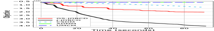
(a) Gisette (3000-100-50)

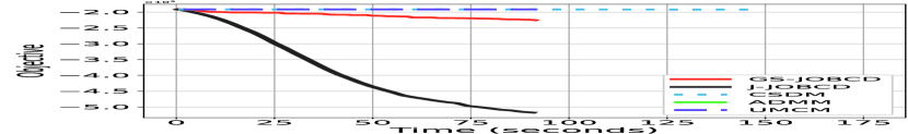
(b) Sector (500-1000-500)

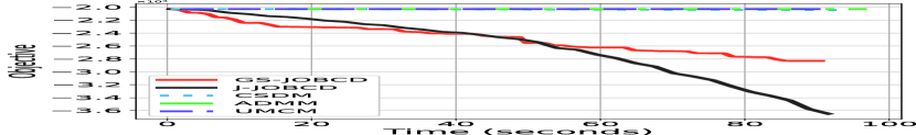
(c) wla (2470-290-145)

Figure 1: The convergence curve for the HEVP across various datasets with different parameters $(m,n,p)$.

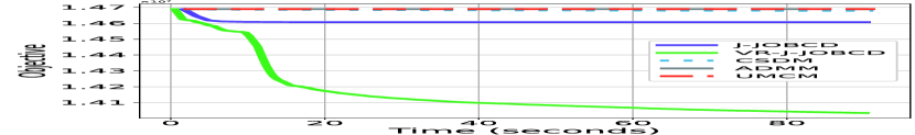
(a) Cifar (10000-50-45)

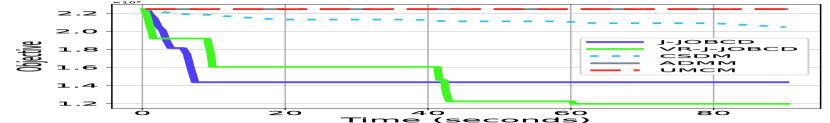
(b) Gisette (6000-50-45)

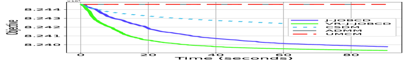
(c) News20 (7967-50-45)

Figure 2: The convergence curve for HSPP across various datasets with different parameters $(m,n,p)$.

$\blacktriangleright$ Experiment Results. Table 1 and Figure 1 display the accuracy and computational efficiency for HEVP, while Figure 2 presents the results for HSPP, leading to the following observations: (i) GS-JOBCD and JJOBCD consistently deliver better performance than the other methods. (ii) Other methods frequently encounter poor local minima, whereas GS-JOBCD effectively escapes these minima and typically achieves lower objective values, aligning with our theory that our methods locate stronger stationary points. (iii) VR-J-JOBCD outperforms both J-JOBCD and CSDM when dealing with a large dataset characterized by an infinite-sum structure.

6 Conclusions

In this paper, we propose a new approach JOBCD, which is based on block coordinate descent, for solving the optimization problem under J-orthogonality constraints. We discuss two specific variants of JOBCD: one based on a Gauss-Seidel strategy (GS-JOBCD), the other on a variance-reduced Jacobi strategy. Both algorithms capitalize on specific structural characteristics of the constraints to converge to more favorable stationary solutions. Notably, VR-J-JOBCD incorporates a variance-reduction technique into a parallel framework to reduce oracle complexity in the minimization of finite-sum functions. For both GS-JOBCD and VR-J-JOBCD, we establish the oracle complexity under mild conditions and strong limit-point convergence results under the Kurdyka-Lojasiewicz inequality. Some experiments on the hyperbolic eigenvalue problem and structural probe problem show the efficiency and efficacy of the proposed methods.

Appendix

The appendix is organized as follows.

Appendix A introduces some notations, technical preliminaries, and relevant lemmas.

Appendix B concludes some additional discussions.

Appendix C presents the proofs for Section 2.

Appendix D offers the proofs for Section 3.

Appendix E contains the proofs for Section 4.

Appendix F contains several extra experiments, extensions and discussions of the proposed methods.

Appendix A Notations, Technical Preliminaries, and Relevant Lemmas

A.1 Notations

In this paper, we denote the Lowercase boldface letters represent vectors, while uppercase letters represent real-valued matrices. We use the Matlab colon notation to denote indices that describe submatrices. The following notations are used throughout this paper.

• $\mathbb{N}$ : Set of natural numbers

• $\mathbb{R}$ : Set of real numbers

• $[n]$: $\{1,2,...,n\}$

• $\|\mathbf{x}\|$: Euclidean norm: $\|\mathbf{x}\|=\|\mathbf{x}\|_{2}=\sqrt{\langle\mathbf{x},\mathbf{x}\rangle}$

• $\mathbf{x}_{i}$: the $i$-th element of vector $\mathbf{x}$

• $\mathbf{X}_{i,j}$ or $\mathbf{X}_{ij}$ : the ($i^{\text{th}}$, $j^{\text{th}}$) element of matrix $\mathbf{X}$

• $\operatorname{vec}(\mathbf{X})$ : $\operatorname{vec}(\mathbf{X})\in\mathbb{R}^{nn\times 1}$, the vector formed by stacking the column vectors of $\mathbf{X}$

• $\operatorname{mat}(\mathbf{x})\in\mathbb{R}^{n\times n}\text{, Convert }\mathbf{x}\in\mathbb{R}^{nn\times 1}\text{ into a matrix with }\operatorname{mat}(\operatorname{vec}(\mathbf{X}))=\mathbf{X}$

• $\mathbf{X}^{\mathsf{T}}$ : the transpose of the matrix $\mathbf{X}$

• $\operatorname{sign}(t)$ : the signum function, $\operatorname{sign}(t)=1$ if $t\geq 0$ and $\operatorname{sign}(t)=-1$ otherwise

• $\mathbf{X}\otimes\mathbf{Y}:$ Kronecker product of $\mathbf{X}$ and $\mathbf{Y}$

• $\text{det}(\mathbf{D})$ : Determinant of a square matrix $\mathbf{D}\in\mathbb{R}^{n\times n}\mathbf{D}\in\mathbb{R}^{n\times n}$

• $\mathbf{C}_{n}^{2}$ : the number of possible combinations choosing $k$ items from $n$ without repetition.

• $\mathbf{0}_{n,r}$ : A zero matrix of size $n\times r$; the subscript is omitted sometimes

• $\mathbf{I}_{r}$ : $\mathbf{I}_{r}\in\mathbb{R}^{r\times r}$, Identity matrix

• $\mathbf{X}\succeq\mathbf{0}(\text{or}~{}\succ\mathbf{0})$ : the Matrix $\mathbf{X}$ is symmetric positive semidefinite (or definite)

• $\operatorname{Diag}(\mathbf{x})$: Diagonal matrix with $\mathbf{x}$ as the main diagonal entries.

• ${\mathbf{tr}}(\mathbf{A})$ : Sum of the elements on the main diagonal $\mathbf{A}$: ${\mathbf{tr}}(\mathbf{A})=\sum_{i}\mathbf{A}_{i,i}$

• $\|\mathbf{X}\|_{*}$ : Nuclear norm: sum of the singular values of matrix $\mathbf{X}$

• $\|\mathbf{X}\|$ : Operator/Spectral norm: the largest singular value of $\mathbf{X}$

• $\|\mathbf{X}\|_{\mathsf{F}}$ : Frobenius norm: $(\sum_{ij}{\mathbf{X}_{ij}^{2}})^{1/2}$

• $\nabla f(\mathbf{X})$ : classical (limiting) Euclidean gradient of $f(\mathbf{X})$ at $\mathbf{X}$

• $\nabla_{\mathcal{J}}f(\mathbf{X})$ : Riemannian gradient of $f(\mathbf{X})$ at $\mathbf{X}$

• $\mathcal{I}_{\mathbf{\xi}}(\mathbf{X})$ : the indicator function of a set $\mathbf{\xi}$ with $\mathcal{I}_{\mathbf{\xi}}(\mathbf{X})=0$ if $\mathbf{X}\in\mathbf{\xi}$ and otherwise $+\infty$

• $\text{dist}(\mathbf{\xi},\mathbf{\xi}^{\prime})$ : the distance between two sets with $\text{dist}(\mathbf{\xi},\mathbf{\xi}^{\prime})\triangleq\inf_{\mathbf{X}\in\mathbf{\xi},\mathbf{X}^{\prime}\in\mathbf{\xi}^{\prime}}\|\mathbf{X}-\mathbf{X}^{\prime}\|_{\mathsf{F}}$

• $\mathcal{I}_{\mathbf{\xi}}(\mathbf{\mathbf{x}})$ : the indicator function of a set $\mathbf{\xi}$ with $\mathcal{I}_{\mathbf{\xi}}(\mathbf{\mathbf{x}})=0$ if $\mathbf{\mathbf{x}}\in\mathbf{\xi}$ and otherwise $+\infty$.

A.2 Relevant Lemmas

Lemma A.1.

(Lemma 6.6 of yuan2023block ) For any $\mathbf{W}\in\mathbb{R}^{n\times n}$, we have: $\sum_{i=1}^{C_{n}^{k}}\|\mathbf{W}(\mathcal{B}_{i},\mathcal{B}_{i})\|_{\mathsf{F}}^{2}=\tfrac{k}{n}C_{n}^{k}\sum_{i}\mathbf{W}_{ii}^{2}+C_{n-2}^{k-2}\sum_{i}\sum_{j,j\neq i}\mathbf{W}_{ij}^{2}$. Here, the set $\{\mathcal{B}_{1},\mathcal{B}_{2},\cdots,\mathcal{B}_{C_{n}^{k}}\}$ represents all possible combinations of the index vectors choosing $k$ items from $n$ without repetition.

Lemma A.2.

We have $\texttt{{{S}}}_{+}$ be the set of $|\texttt{{{S}}}_{+}|=b$ samples from $[N]$, drawn with replacement and uniformly at random. Then, $\forall t,\mathbf{X}^{t}\in\mathbb{R}^{n\times n}$, we have:

$${\textstyle\mathbb{E}_{\iota^{t}}[\|\frac{1}{b}\sum_{i\in\texttt{{{S}}}_{+}}\nabla f_{i}(\mathbf{X}^{t})-\nabla f(\mathbf{X}^{t})\|_{\mathsf{F}}^{2}]=\frac{N-b}{b(N-1)}\mathbb{E}_{\iota^{t}}[\|\nabla f_{i}(\mathbf{X}^{t})-\nabla f(\mathbf{X}^{t})\|_{\mathsf{F}}^{2}].}$$

Proof.

The proof is exactly the same as in Lemma 2.8 of cai2023cyclic . ∎

Lemma A.3.

The tangent space ${\textstyle\mathbf{T}_{\mathbf{X}}\mathcal{J}}$ of manifold constructed by ${\textstyle\mathbf{X}^{\top}\mathbf{J}\mathbf{X}=\mathbf{J}}$, with $\mathbf{X}\in\mathbb{R}^{n\times n}$, is :

$${\textstyle\mathbf{T}_{\mathbf{X}}\mathcal{J}}\triangleq{\textstyle\{\mathbf{Y}\in\mathbb{R}^{n\times n}\mid\mathbf{X}^{\top}\mathbf{J}\mathbf{Y}+\mathbf{Y}^{\top}\mathbf{J}\mathbf{X}=0\}},$$ (15)

where $\mathbf{Y}=t\tilde{\mathbf{Y}}$ with $t$ is a positive scalar approaching 0.

Proof.

Assuming point $\mathbf{X}\in\mathbb{R}^{n\times n}$ lies on manifold $\mathcal{J}$, we have: ${\textstyle h(\mathbf{X})=\mathbf{X}^{\top}\mathbf{J}\mathbf{X}-\mathbf{J}}$. Moving along $\mathbf{Y}\in\mathbb{R}^{n\times n}$ in the tangent space of $\mathbf{X}$, we obtain:

$${\textstyle h(\mathbf{X+Y})}= {\textstyle(\mathbf{X+Y})^{\top}\mathbf{J}(\mathbf{X+Y})-\mathbf{J}}$$

$$= {\textstyle\mathbf{X}^{\top}\mathbf{J}\mathbf{X}+\mathbf{X}^{\top}\mathbf{J}\mathbf{Y}+\mathbf{Y}^{\top}\mathbf{J}\mathbf{X}+\mathbf{Y}^{\top}\mathbf{J}\mathbf{Y}-\mathbf{J}}$$

$$\stackrel{{\scriptstyle\text{\char 172}}}{{=}} {\textstyle\mathbf{X}^{\top}\mathbf{J}\mathbf{Y}+\mathbf{Y}^{\top}\mathbf{J}\mathbf{X}+\mathbf{Y}^{\top}\mathbf{J}\mathbf{Y}}$$

$$\stackrel{{\scriptstyle\text{\char 173}}}{{=}} {\textstyle t\mathbf{X}^{\top}\mathbf{J}\tilde{\mathbf{Y}}+t\tilde{\mathbf{Y}}^{\top}\mathbf{J}\mathbf{X}+t^{2}\tilde{\mathbf{Y}}^{\top}\mathbf{J}\tilde{\mathbf{Y}}}$$

where step ① uses ${\textstyle\mathbf{X}^{\top}\mathbf{J}\mathbf{X}=\mathbf{J}}$; step ② uses $\mathbf{Y}=t\tilde{\mathbf{Y}}$.

Since $t$ is a positive scalar approaching 0, we can ignore the higher-order term: $t^{2}\tilde{\mathbf{Y}}^{\top}\mathbf{J}\tilde{\mathbf{Y}}$. According to the properties of the tangent space of any manifold, we have: ${\textstyle h(\mathbf{X+Y})=0}$, In other words, $\mathbf{X}^{\top}\mathbf{J}\mathbf{Y}+\mathbf{Y}^{\top}\mathbf{J}\mathbf{X}=0$, i.e. we obtain the defining equation for the tangent space: ${\textstyle\mathbf{T}_{\mathbf{X}}\mathcal{J}\triangleq\{\mathbf{Y}\in\mathbb{R}^{n\times n}\mid\mathbf{X}^{\top}\mathbf{J}\mathbf{Y}+\mathbf{Y}^{\top}\mathbf{J}\mathbf{X}=0\}}$. ∎

Appendix B Additional Discussions

B.1 On the Global Optimal Solution for Problem (7)

In Section 2.1, we have demonstrated how to use the breakpoint search method to obtain an optimal solution for the case of $\mathbf{V}=(\begin{smallmatrix}\operatorname{\tilde{c}}&\operatorname{\tilde{s}}\\ \operatorname{\tilde{s}}&\operatorname{\tilde{c}}\end{smallmatrix})$ of Problem (7). Since the structure of the other three cases $\mathbf{V}\in\{(\begin{smallmatrix}\operatorname{\tilde{c}}&~{}-\operatorname{\tilde{s}}\\ -\operatorname{\tilde{s}}&~{}\operatorname{\tilde{c}}\end{smallmatrix}),(\begin{smallmatrix}-\operatorname{\tilde{c}}&~{}-\operatorname{\tilde{s}}\\ \operatorname{\tilde{s}}&~{}\operatorname{\tilde{c}}\end{smallmatrix}),(\begin{smallmatrix}\operatorname{\tilde{c}}&~{}-\operatorname{\tilde{s}}\\ \operatorname{\tilde{s}}&~{}-\operatorname{\tilde{c}}\end{smallmatrix})\}$ is exactly the same except for the coefficients of Problem (8), we will provide the corresponding coefficients in Problem (8): $\min_{\operatorname{\tilde{c}},\operatorname{\tilde{s}}}a\operatorname{\tilde{c}}+b\operatorname{\tilde{s}}+c\operatorname{\tilde{c}}^{2}+d\operatorname{\tilde{c}}\operatorname{\tilde{s}}+e\operatorname{\tilde{s}}^{2}$, and omit the specific analysis process.

Case (a). $\mathbf{V}=(\begin{smallmatrix}\operatorname{\tilde{c}}&~{}-\operatorname{\tilde{s}}\\ -\operatorname{\tilde{s}}&~{}\operatorname{\tilde{c}}\end{smallmatrix})$: $a=\mathbf{P}_{11}+\mathbf{P}_{22}$, $b=-\mathbf{P}_{12}-\mathbf{P}_{21}$, $c=\tfrac{1}{2}(\dot{\mathbf{Q}}_{11}+\dot{\mathbf{Q}}_{41}+\dot{\mathbf{Q}}_{14}+\dot{\mathbf{Q}}_{44})$, $d=-\tfrac{1}{2}(\dot{\mathbf{Q}}_{21}+\dot{\mathbf{Q}}_{31}+\dot{\mathbf{Q}}_{12}+\dot{\mathbf{Q}}_{42}+\dot{\mathbf{Q}}_{13}+\dot{\mathbf{Q}}_{43}+\dot{\mathbf{Q}}_{24}+\dot{\mathbf{Q}}_{34})$, and $e=\tfrac{1}{2}(\dot{\mathbf{Q}}_{22}+\dot{\mathbf{Q}}_{32}+\dot{\mathbf{Q}}_{23}+\dot{\mathbf{Q}}_{33})$.

Case (b). $\mathbf{V}=(\begin{smallmatrix}-\operatorname{\tilde{c}}&~{}-\operatorname{\tilde{s}}\\ \operatorname{\tilde{s}}&~{}\operatorname{\tilde{c}}\end{smallmatrix})$:$a=-\mathbf{P}_{11}+\mathbf{P}_{22}$, $b=-\mathbf{P}_{12}+\mathbf{P}_{21}$, $c=\tfrac{1}{2}(\dot{\mathbf{Q}}_{11}-\dot{\mathbf{Q}}_{41}-\dot{\mathbf{Q}}_{14}+\dot{\mathbf{Q}}_{44})$, $d=\tfrac{1}{2}(\dot{\mathbf{Q}}_{21}-\dot{\mathbf{Q}}_{31}+\dot{\mathbf{Q}}_{12}-\dot{\mathbf{Q}}_{42}-\dot{\mathbf{Q}}_{13}+\dot{\mathbf{Q}}_{43}-\dot{\mathbf{Q}}_{24}+\dot{\mathbf{Q}}_{34})$, and $e=\tfrac{1}{2}(\dot{\mathbf{Q}}_{22}-\dot{\mathbf{Q}}_{32}-\dot{\mathbf{Q}}_{23}+\dot{\mathbf{Q}}_{33})$.

Case (c). $\mathbf{V}=(\begin{smallmatrix}\operatorname{\tilde{c}}&~{}-\operatorname{\tilde{s}}\\ \operatorname{\tilde{s}}&~{}-\operatorname{\tilde{c}}\end{smallmatrix})$:$a=\mathbf{P}_{11}-\mathbf{P}_{22}$, $b=-\mathbf{P}_{12}+\mathbf{P}_{21}$, $c=\tfrac{1}{2}(\dot{\mathbf{Q}}_{11}-\dot{\mathbf{Q}}_{41}-\dot{\mathbf{Q}}_{14}+\dot{\mathbf{Q}}_{44})$, $d=\tfrac{1}{2}(-\dot{\mathbf{Q}}_{21}+\dot{\mathbf{Q}}_{31}-\dot{\mathbf{Q}}_{12}+\dot{\mathbf{Q}}_{42}+\dot{\mathbf{Q}}_{13}-\dot{\mathbf{Q}}_{43}+\dot{\mathbf{Q}}_{24}-\dot{\mathbf{Q}}_{34})$, and $e=\tfrac{1}{2}(\dot{\mathbf{Q}}_{22}-\dot{\mathbf{Q}}_{32}-\dot{\mathbf{Q}}_{23}+\dot{\mathbf{Q}}_{33})$.

Appendix C Proofs for Section 2

C.1 Proof of Lemma 2.1

Proof.

Defining $\mathbf{J}_{\texttt{{B}}\texttt{{B}}}=\mathbf{J}(\mathbf{U}_{\texttt{{B}}},\mathbf{U}_{\texttt{{B}}})$ , then we have: $\mathbf{J}\mathbf{U}_{\texttt{{B}}}=\mathbf{U}_{\texttt{{B}}}\mathbf{J}_{\texttt{{B}}\texttt{{B}}}$, $\mathbf{U}_{\texttt{{B}}}^{\top}\mathbf{J}=\mathbf{J}_{\texttt{{B}}\texttt{{B}}}\mathbf{U}_{\texttt{{B}}}^{\top}$, and $\mathbf{U}_{\texttt{{B}}}^{\top}\mathbf{J}\mathbf{U}_{\texttt{{B}}}=\mathbf{J}_{\texttt{{B}}\texttt{{B}}}$.

Part (a). For any $\mathbf{V}\in\mathbb{R}^{2\times 2}$ and $\texttt{{B}}\in\{\mathcal{B}_{i}\}_{i=1}^{\mathbf{C}_{n}^{2}}$, we have:

$${[\mathbf{X}^{+}]^{\top}\mathbf{J}\mathbf{X}^{+}-\mathbf{X}^{\top}\mathbf{J}\mathbf{X}}$$

$$\stackrel{{\scriptstyle\text{\char 172}}}{{=}} \mathbf{X}^{\top}\mathbf{J}\mathbf{U}_{\texttt{{B}}}(\mathbf{V}-\mathbf{I}_{2})\mathbf{U}_{\texttt{{B}}}^{\top}\mathbf{X}+[\mathbf{U}_{\texttt{{B}}}(\mathbf{V}-\mathbf{I}_{2})\mathbf{U}_{\texttt{{B}}}^{\top}\mathbf{X}]^{\top}\mathbf{J}\mathbf{X}$$

$$+[\mathbf{U}_{\texttt{{B}}}(\mathbf{V}-\mathbf{I}_{2})\mathbf{U}_{\texttt{{B}}}^{\top}\mathbf{X}]^{\top}\mathbf{J}[\mathbf{U}_{\texttt{{B}}}(\mathbf{V}-\mathbf{I}_{2})\mathbf{U}_{\texttt{{B}}}^{\top}\mathbf{X}]$$

$$= \mathbf{X}^{\top}[\mathbf{J}\mathbf{U}_{\texttt{{B}}}(\mathbf{V}-\mathbf{I}_{2})\mathbf{U}_{\texttt{{B}}}^{\top}+\mathbf{U}_{\texttt{{B}}}(\mathbf{V}-\mathbf{I}_{2})^{\top}\mathbf{U}_{\texttt{{B}}}^{\top}\mathbf{J}+\mathbf{U}_{\texttt{{B}}}(\mathbf{V}-\mathbf{I}_{2})^{\top}\mathbf{U}_{\texttt{{B}}}^{\top}\mathbf{J}\mathbf{U}_{\texttt{{B}}}(\mathbf{V}-\mathbf{I}_{2})\mathbf{U}_{\texttt{{B}}}^{\top}]\mathbf{X}$$

$$= \mathbf{X}^{\top}[\mathbf{U}_{\texttt{{B}}}\mathbf{J}_{\texttt{{B}}\texttt{{B}}}(\mathbf{V}-\mathbf{I}_{2})\mathbf{U}_{\texttt{{B}}}^{\top}+\mathbf{U}_{\texttt{{B}}}(\mathbf{V}-\mathbf{I}_{2})^{\top}\mathbf{J}_{\texttt{{B}}\texttt{{B}}}\mathbf{U}_{\texttt{{B}}}^{\top}+\mathbf{U}_{\texttt{{B}}}(\mathbf{V}-\mathbf{I}_{2})^{\top}\mathbf{J}_{\texttt{{B}}\texttt{{B}}}(\mathbf{V}-\mathbf{I}_{2})\mathbf{U}_{\texttt{{B}}}^{\top}]\mathbf{X}$$

$$= \mathbf{X}^{\top}\mathbf{U}_{\texttt{{B}}}[\mathbf{J}_{\texttt{{B}}\texttt{{B}}}(\mathbf{V}-\mathbf{I}_{2})+(\mathbf{V}-\mathbf{I}_{2})^{\top}\mathbf{J}_{\texttt{{B}}\texttt{{B}}}+(\mathbf{V}-\mathbf{I}_{2})^{\top}\mathbf{J}_{\texttt{{B}}\texttt{{B}}}(\mathbf{V}-\mathbf{I}_{2})]\mathbf{U}_{\texttt{{B}}}^{\top}\mathbf{X}$$

$$= \mathbf{X}^{\top}\mathbf{U}_{\texttt{{B}}}[\mathbf{V}^{\top}\mathbf{J}_{\texttt{{B}}\texttt{{B}}}\mathbf{V}-\mathbf{J}_{\texttt{{B}}\texttt{{B}}}]\mathbf{U}_{\texttt{{B}}}^{\top}\mathbf{X}$$

$$\stackrel{{\scriptstyle\text{\text{\char 173}}}}{{=}} \mathbf{0}.$$

Part (b). Using the update rule for ${\textstyle\mathbf{X}^{+}=\mathbf{X}+\mathbf{U}_{\texttt{{B}}}(\mathbf{V}-\mathbf{I}_{2})\mathbf{U}_{\texttt{{B}}}^{\top}\mathbf{X}\in\mathbb{R}^{n\times n}}$, we derive:

$${\textstyle\|\mathbf{X}^{+}-\mathbf{X}\|_{\mathsf{F}}} = {\textstyle\|\mathbf{U}_{\texttt{{B}}}(\mathbf{V}-\mathbf{I}_{2})\mathbf{U}_{\texttt{{B}}}^{\top}\mathbf{X}\|_{\mathsf{F}}}$$

$$\stackrel{{\scriptstyle\text{\char 172}}}{{\leq}} {\textstyle\|\mathbf{U}_{\texttt{{B}}}\|_{\mathsf{F}}\cdot\|(\mathbf{V}-\mathbf{I}_{2})\mathbf{U}_{\texttt{{B}}}^{\top}\mathbf{X}\|_{\mathsf{F}}},$$

$$\stackrel{{\scriptstyle\text{\char 173}}}{{\leq}} {\textstyle\|\mathbf{U}_{\texttt{{B}}}\|_{\mathsf{F}}\cdot\|(\mathbf{V}-\mathbf{I}_{2})\|_{\mathsf{F}}\cdot\|\mathbf{U}_{\texttt{{B}}}^{\top}\|_{\mathsf{F}}\cdot\|\mathbf{X}\|_{\mathsf{F}}},$$

$$\stackrel{{\scriptstyle\text{\char 174}}}{{=}} {\textstyle\|\mathbf{V}-\mathbf{I}_{2}\|_{\mathsf{F}}\cdot\|\mathbf{X}\|_{\mathsf{F}}},$$

where step ① and step ② use the norm inequality that ${\textstyle\|\mathbf{AX}\|_{\mathsf{F}}\leq\|\mathbf{A}\|_{\mathsf{F}}\cdot\|\mathbf{X}\|_{\mathsf{F}}}$ for any $\mathbf{A}$ and $\mathbf{X}$; step ③ uses ${\textstyle\|\mathbf{U}_{\texttt{{B}}}\|=\|\mathbf{U}_{\texttt{{B}}}^{\top}\|=1}$.

Part (c). We define $\mathbf{Z}\triangleq\mathbf{U}_{\texttt{{B}}}^{\top}\mathbf{X}$. We derive:

$$\|\mathbf{X}^{+}-\mathbf{X}\|_{\mathbf{H}}^{2} {=} {\textstyle\|\mathbf{U}_{\texttt{{B}}}(\mathbf{V}-\mathbf{I}_{2})\mathbf{Z}\|_{\mathbf{H}}^{2}}$$

$$\stackrel{{\scriptstyle\text{\char 172}}}{{=}} \text{vec}(\mathbf{U}_{\texttt{{B}}}(\mathbf{V}-\mathbf{I}_{2})\mathbf{Z})^{\top}\mathbf{H}\text{vec}(\mathbf{U}_{\texttt{{B}}}(\mathbf{V}-\mathbf{I}_{2})\mathbf{Z})$$

$$\stackrel{{\scriptstyle\text{\char 173}}}{{=}} \text{vec}(\mathbf{V}-\mathbf{I}_{2})^{\top}(\mathbf{Z}^{\top}\otimes\mathbf{U}_{\texttt{{B}}})^{\top}\mathbf{H}(\mathbf{Z}^{\top}\otimes\mathbf{U}_{\texttt{{B}}})\text{vec}(\mathbf{V}-\mathbf{I}_{2})$$

$$= \|\mathbf{V}-\mathbf{I}_{2}\|^{2}_{(\mathbf{Z}^{\top}\otimes\mathbf{U}_{\texttt{{B}}})^{\top}\mathbf{H}(\mathbf{Z}^{\top}\otimes\mathbf{U}_{\texttt{{B}}})}$$

$$\stackrel{{\scriptstyle\text{\char 174}}}{{\leq}} \|\mathbf{V}-\mathbf{I}_{2}\|^{2}_{\mathbf{Q}},$$

where step ① uses $\|\mathbf{X}\|^{2}_{\mathbf{H}}=\text{vec}(\mathbf{X})^{\top}\mathbf{H}\text{vec}(\mathbf{X})$; step ② uses $(\mathbf{Z}^{\top}\otimes\mathbf{R})\text{vec}(\textbf{U})=\text{vec}(\mathbf{R}\mathbf{U}\mathbf{Z})$ for all $\mathbf{R}$, $\mathbf{Z}$ and $\mathbf{U}$ of suitable dimensions; step ③ uses the choice of $\mathbf{Q}\succcurlyeq\underline{\mathbf{Q}}\triangleq(\mathbf{Z}^{\top}\otimes\mathbf{U}_{\texttt{{B}}})^{\top}\mathbf{H}(\mathbf{Z}^{\top}\otimes\mathbf{U}_{\texttt{{B}}})$. ∎

C.2 Proof of Lemma 2.3

Proof.

We denote $w=c+e$. According to the properties of trigonometric functions, we have: (i) $\operatorname{\tilde{c}}^{2}=\tfrac{1}{1-\operatorname{\tilde{t}}^{2}}$; (ii) $\operatorname{\tilde{s}}^{2}=\tfrac{\operatorname{\tilde{t}}^{2}}{1-\operatorname{\tilde{t}}^{2}}$; (iii)$\operatorname{\tilde{t}}=\tfrac{\operatorname{\tilde{s}}}{\operatorname{\tilde{c}}}$, leading to: ${\textstyle\operatorname{\tilde{c}}=\frac{\pm 1}{\sqrt{1-\operatorname{\tilde{t}}^{2}}},\operatorname{\tilde{s}}=\frac{\pm\operatorname{\tilde{t}}}{\sqrt{1-\operatorname{\tilde{t}}^{2}}}}$ with $|\operatorname{\tilde{t}}|<1$.

We discuss two cases for Problem (8).

Case (a). ${\textstyle\operatorname{\tilde{c}}=\frac{1}{\sqrt{1-\operatorname{\tilde{t}}^{2}}},\operatorname{\tilde{s}}=\frac{\operatorname{\tilde{t}}}{\sqrt{1-\operatorname{\tilde{t}}^{2}}}}$. Problem (8) is equivalent to the following problem: $\bar{\mu}_{+}=\arg\min_{\mu}\frac{a+\operatorname{\tilde{t}}b}{\sqrt{1-\operatorname{\tilde{t}}^{2}}}+\frac{w+\operatorname{\tilde{t}}d}{1-\operatorname{\tilde{t}}^{2}}-e$. Therefore, the optimal solution $\bar{\mu}_{+}$can be computed as:

$${\textstyle\cosh(\bar{\mu}_{+})=\frac{1}{\sqrt{1-(\bar{t}_{+})^{2}}},~{}\text{and}~{}\sinh(\bar{\mu}_{+})=\frac{\bar{t}_{+}}{\sqrt{1-(\bar{t}_{+})^{2}}}}$$ (16)

Case (b). ${\textstyle\operatorname{\tilde{c}}=\frac{-1}{\sqrt{1-\operatorname{\tilde{t}}^{2}}},\operatorname{\tilde{s}}=\frac{-\operatorname{\tilde{t}}}{\sqrt{1-\operatorname{\tilde{t}}^{2}}}}$. Problem (8) is equivalent to the following problem: $\bar{\mu}_{-}=\arg\min_{\mu}\frac{-a-\operatorname{\tilde{t}}b}{\sqrt{1-\operatorname{\tilde{t}}^{2}}}+\frac{w+\operatorname{\tilde{t}}d}{1-\operatorname{\tilde{t}}^{2}}-e$. Therefore, the optimal solution $\bar{\mu}_{-}$can be computed as:

$${\textstyle\cosh(\bar{\mu}_{-})=\frac{-1}{\sqrt{1-(\bar{t}_{-})^{2}}},~{}\text{and}~{}\sinh(\bar{\mu}_{-})=\frac{-\bar{t}_{-}}{\sqrt{1-(\bar{t}_{-})^{2}}}}.$$ (17)

We define the objective function as: ${\textstyle\breve{F}(\tilde{c},\tilde{s})}\triangleq{\textstyle a\tilde{c}+b\tilde{s}+c\tilde{c}^{2}+d\tilde{c}\tilde{s}+e\tilde{s}^{2}}$. In view of (16) and (17), the optimal solution pair $[cosh(\bar{\mu},sinh(\bar{\mu})]$ for problem (8) can be computed as:

$$[\cosh(\bar{\mu}),\sinh(\bar{\mu})]=\arg\min_{[c,s]}\breve{F}(c,s),$$

$$~{}\operatorname{s.t.}~{}[c,s]\in\{[\cosh(\bar{\mu}_{+}),\sinh(\bar{\mu}_{+})],[\cosh(\bar{\mu}_{-}),\sinh(\bar{\mu}_{-})]\}$$

Importantly, it is not necessary to compute the values $\bar{\mu}_{+}$ for (16) and $\bar{\mu}_{-}$ for (17).

∎

C.3 Proof of Lemma 2.4

Proof.

The objective function for $\texttt{{B}}_{(i)}^{t}$ as in Equation (3) is formulated as :

$$\textstyle f(\mathbf{X}^{t})+\tfrac{1}{2}\|\mathbf{V}_{i}-\mathbf{I}\|_{\mathbf{Q}+\theta\mathbf{I}}^{2}+\langle\mathbf{V}_{i}-\mathbf{I},[\nabla f(\mathbf{X}^{t})(\mathbf{X}^{t})^{\mathsf{T}}]_{\texttt{{B}}_{(i)}^{t}\texttt{{B}}_{(i)}^{t}}\rangle$$

Part (1). For the part of ${\textstyle\frac{1}{2}\|\mathbf{V}_{i}-\mathbf{I}\|_{\mathbf{Q}+\theta\mathbf{I}}^{2}}$, it is obviously irrelevant.

Part (2). For the part of $\langle\mathbf{V}_{i}-\mathbf{I},[\nabla f(\mathbf{X}^{t})(\mathbf{X}^{t})^{\mathsf{T}}]_{\texttt{{B}}_{(i)}^{t}\texttt{{B}}_{(i)}^{t}}\rangle$, we note that $[\nabla f(\mathbf{X}^{t})(\mathbf{X}^{t})^{\top}]_{\texttt{{B}}_{(i)}^{t}\texttt{{B}}_{(i)}^{t}}=[\nabla f(\mathbf{X}^{t})]{(\texttt{{B}}_{(i)}^{t},:)}[(\mathbf{X}^{t})^{\top}]{(:,\texttt{{B}}_{(i)}^{t})}=[\nabla f(\mathbf{X}^{t})]{(\texttt{{B}}_{(i)}^{t},:)}[(\mathbf{X}^{t}){(\texttt{{B}}_{(i)}^{t},:)}]^{\top}$ , which just use the information of block $\texttt{{B}}_{(i)}^{t}$. The proof ends. ∎

C.4 Proof of Lemma 2.5

Proof.

Part (a). For the purpose of analysis, we define the following: $\forall i\in[\frac{n}{2}],\mathbf{K}_{i}=\mathbf{U}_{\texttt{{B}}_{(i)}}(\mathbf{V}_{i}-\mathbf{I}_{2})\mathbf{U}_{\texttt{{B}}_{(i)}}^{\top}\mathbf{X}$.

$$\textstyle\|\sum_{i=1}^{\frac{n}{2}}[\mathbf{U}_{\texttt{{B}}_{(i)}}(\mathbf{V}_{i}-\mathbf{I}_{2})\mathbf{U}_{\texttt{{B}}_{(i)}}^{\top}\mathbf{X}]\|_{\mathsf{F}}^{2} \stackrel{{\scriptstyle\text{\char 172}}}{{=}} \left\|\left[\begin{array}[]{c}\mathbf{K}_{1}\\ \mathbf{K}_{2}\\ \vdots\\ \mathbf{K}_{\frac{n}{2}}\end{array}\right]\right\|_{\mathsf{F}}^{2}$$

$$\stackrel{{\scriptstyle\text{\char 173}}}{{=}} {\textstyle\|\mathbf{K}_{1}\|_{\mathsf{F}}^{2}+\|\mathbf{K}_{2}\|_{\mathsf{F}}^{2}+\cdots+\|\mathbf{K}_{\frac{n}{2}}\|_{\mathsf{F}}^{2}}$$

$$\stackrel{{\scriptstyle\text{\char 174}}}{{=}} {\textstyle\sum_{i=1}^{\frac{n}{2}}[\|\mathbf{U}_{\texttt{{B}}_{(i)}}(\mathbf{V}_{i}-\mathbf{I}_{2})\mathbf{U}_{\texttt{{B}}_{(i)}}^{\top}\mathbf{X}\|_{\mathsf{F}}^{2}]}$$

where step ① uses the definition of $\mathbf{K}_{i}$ and the assumption that $\texttt{{B}}\in\Upsilon$; step ② uses the definition of Squared Frobenius Norm; step ③ uses the definition of $\mathbf{K}_{i}$.

Part (b). Using the update rule for ${\textstyle\mathbf{X}^{+}=\mathbf{X}+[\sum_{i=1}^{n/2}\mathbf{U}_{\texttt{{B}}_{(i)}}(\mathbf{V}_{i}-\mathbf{I}_{2})\mathbf{U}_{\texttt{{B}}_{(i)}}^{\top}]\mathbf{X}\in\mathbb{R}^{n\times n}}$, we have the following inequalities:

$${\textstyle\|\mathbf{X}^{+}-\mathbf{X}\|_{\mathsf{F}}^{2}} = {\textstyle\|[\sum_{i=1}^{n/2}\mathbf{U}_{\texttt{{B}}_{(i)}}(\mathbf{V}_{i}-\mathbf{I}_{2})\mathbf{U}_{\texttt{{B}}_{(i)}}^{\top}]\mathbf{X}\|_{\mathsf{F}}^{2}}$$ (23)

$$\stackrel{{\scriptstyle\text{\char 172}}}{{=}} {\textstyle\sum_{i=1}^{n/2}\|[\mathbf{U}_{\texttt{{B}}_{(i)}}(\mathbf{V}_{i}-\mathbf{I}_{2})\mathbf{U}_{\texttt{{B}}_{(i)}}^{\top}]\mathbf{X}\|_{\mathsf{F}}^{2}}$$ (24)

$$\stackrel{{\scriptstyle\text{\char 173}}}{{\leq}} {\textstyle\sum_{i=1}^{n/2}\|\mathbf{V}_{i}-\mathbf{I}_{2}\|_{\mathsf{F}}^{2}\cdot\|\mathbf{X}\|_{\mathsf{F}}^{2}},$$ (25)

where step ① uses the conclusion of Part (a); step ② uses the same proof process of Part (b) of lemma 2.1.

Part (c). We derive the following results:

$$\frac{1}{2}\|\mathbf{X}^{+}-\mathbf{X}\|_{\mathbf{H}}^{2} ={\textstyle\frac{1}{2}\|[\sum_{i=1}^{n/2}\mathbf{U}_{\texttt{{B}}_{(i)}}(\mathbf{V}_{i}-\mathbf{I}_{2})\mathbf{U}_{\texttt{{B}}_{(i)}}^{\top}]\mathbf{X}\|_{\mathbf{H}}^{2}}$$

$$\stackrel{{\scriptstyle\text{\char 172}}}{{=}}{\textstyle\frac{1}{2}\sum_{i=1}^{n/2}\|[\mathbf{U}_{\texttt{{B}}_{(i)}}(\mathbf{V}_{i}-\mathbf{I}_{2})\mathbf{U}_{\texttt{{B}}_{(i)}}^{\top}]\mathbf{X}\|_{\mathbf{H}}^{2}}$$

$$\stackrel{{\scriptstyle\text{\char 173}}}{{\leq}}{\textstyle\frac{1}{2}\sum_{i=1}^{n/2}\|\mathbf{V}_{i}-\mathbf{I}_{2}\|_{\mathbf{Q}}^{2}}$$

where step ① uses the conclusion of Part (a); step ② uses the same proof process of Part (c) of lemma 2.1.

Part (d). We derive the following results:

$${\textstyle\sum_{i=1}^{n/2}\langle\mathbf{V}_{i}-\mathbf{I}_{2},[(\nabla f(\mathbf{X})-\tilde{\mathbf{G}}){\mathbf{X}}^{\top}]_{\texttt{{B}}_{\mathbf{i}}\texttt{{B}}_{\mathbf{i}}}\rangle}$$ (26)

$$= {\textstyle\sum_{i=1}^{n/2}\langle[\mathbf{U}_{\texttt{{B}}_{(i)}}(\mathbf{V}_{i}-\mathbf{I}_{2})\mathbf{U}_{\texttt{{B}}_{(i)}}^{\top}]\mathbf{X},[(\nabla f(\mathbf{X})-\tilde{\mathbf{G}})]\rangle}$$

$$= {\textstyle\langle\mathbf{X}^{+}-\mathbf{X},[(\nabla f(\mathbf{X})-\tilde{\mathbf{G}})]\rangle}$$

$$\stackrel{{\scriptstyle\text{\char 172}}}{{\leq}} {\textstyle\frac{1}{2}\|\mathbf{X}^{+}-\mathbf{X}\|^{2}_{\mathsf{F}}+\frac{1}{2}\|[\nabla f(\mathbf{X})-\tilde{\mathbf{G}}]\|^{2}_{\mathsf{F}}}$$

$$\stackrel{{\scriptstyle\text{\char 173}}}{{\leq}} {\textstyle\frac{1}{2}\|\mathbf{X}\|_{\mathsf{F}}^{2}\sum_{i=1}^{n/2}\|\mathbf{V}_{i}-\mathbf{I}_{2}\|_{\mathsf{F}}^{2}+\frac{1}{2}\|[\nabla f(\mathbf{X})-\tilde{\mathbf{G}}]\|^{2}_{\mathsf{F}}}$$

where step ① uses $\forall\mathbf{A},\mathbf{B},\frac{1}{2}\|\mathbf{A}-\mathbf{B}\|^{2}_{\mathsf{F}}=\frac{1}{2}\|\mathbf{A}\|^{2}_{\mathsf{F}}+\frac{1}{2}\|\mathbf{B}\|^{2}_{\mathsf{F}}-\langle\mathbf{A},\mathbf{B}\rangle\geq 0$, with $\mathbf{A}=\|\mathbf{X}^{+}-\mathbf{X}\|^{2}_{\mathsf{F}}$ and $\mathbf{B}=\|[\nabla f(\mathbf{X})-\tilde{\mathbf{G}}]\|^{2}_{\mathsf{F}}$; step ② uses the conclusion of Part (b). ∎

Appendix D Proofs for Section 3

D.1 Proof of Lemma 3.1

Proof.

We consider the Lagrangian function of problem (1):

$$\mathcal{L}(\mathbf{X},\Lambda)=f(\mathbf{X})-\tfrac{1}{2}\langle\Lambda,\mathbf{X}^{\mathsf{T}}\mathbf{J}\mathbf{X}-\mathbf{J}\rangle.$$ (27)

Setting the gradient of $\mathcal{L}(\mathbf{X},\Lambda)$ w.r.t. $\mathbf{X}$ to zero yields:

$$\nabla f(\mathbf{X})-\mathbf{J}\mathbf{X}\Lambda=\mathbf{0}.$$ (28)

Part (a). Multiplying both sides by $\mathbf{X}^{\mathsf{T}}$ and using the fact that $\mathbf{X}^{\mathsf{T}}\mathbf{J}\mathbf{X}=\mathbf{J}$, we have $\mathbf{J}\Lambda=\mathbf{X}^{\mathsf{T}}\nabla f(\mathbf{X})$. Multiplying both sides by $\mathbf{J}^{\mathsf{T}}$ and using $\mathbf{J}^{\top}\mathbf{J}=\mathbf{I}$, we have $\Lambda=\mathbf{J}\mathbf{X}^{\top}\nabla f(\mathbf{X})$. Since $\Lambda$ is symmetric, we have $\Lambda=\nabla f(\mathbf{X})^{\mathsf{T}}\mathbf{X}\mathbf{J}$. Putting this equality into Equality (28) yields the following first-order optimality condition for Problem (1):

$$\nabla f(\mathbf{X})=\mathbf{J}\mathbf{X}[\nabla f(\mathbf{X})]^{\mathsf{T}}\mathbf{X}\mathbf{J}.$$ (29)

Part (b). We let $\mathbf{G}=\nabla f(\mathbf{X})$. We derive the following results:

$$\mathbf{G}=\mathbf{J}\mathbf{X}\mathbf{G}^{\mathsf{T}}\mathbf{X}\mathbf{J} \stackrel{{\scriptstyle\text{\char 172}}}{{\Rightarrow}} \mathbf{J}\mathbf{X}^{\mathsf{T}}\cdot\mathbf{G}=\mathbf{J}\mathbf{X}^{\mathsf{T}}\cdot\mathbf{J}\mathbf{X}\mathbf{G}^{\mathsf{T}}\mathbf{X}\mathbf{J}$$

$$\stackrel{{\scriptstyle\text{\char 173}}}{{\Rightarrow}} \mathbf{J}\mathbf{X}^{\mathsf{T}}\mathbf{G}=\mathbf{G}^{\mathsf{T}}\mathbf{X}\mathbf{J}$$

$$\stackrel{{\scriptstyle\text{\char 174}}}{{\Rightarrow}} \mathbf{X}(\mathbf{J}\mathbf{X}^{\mathsf{T}}\mathbf{G})\mathbf{X}^{\mathsf{T}}=\mathbf{X}(\mathbf{G}^{\mathsf{T}}\mathbf{X}\mathbf{J})\mathbf{X}^{\mathsf{T}}$$

$$\stackrel{{\scriptstyle\text{\char 175}}}{{\Rightarrow}} \mathbf{X}\underbrace{\mathbf{J}\mathbf{X}^{\mathsf{T}}\mathbf{G}\mathbf{X}^{\mathsf{T}}\mathbf{J}}_{\triangleq\mathbf{G}^{\mathsf{T}}}\mathbf{J}=\mathbf{J}\underbrace{\mathbf{J}\mathbf{X}\mathbf{G}^{\mathsf{T}}\mathbf{X}\mathbf{J}}_{\triangleq\mathbf{G}}\mathbf{X}^{\mathsf{T}}$$

$$\stackrel{{\scriptstyle\text{\char 176}}}{{\Rightarrow}} (\mathbf{X}\mathbf{G}^{\mathsf{T}}\mathbf{J})\cdot\mathbf{J}\mathbf{X}=(\mathbf{J}\mathbf{G}\mathbf{X}^{\mathsf{T}})\cdot\mathbf{J}\mathbf{X}$$

$$\stackrel{{\scriptstyle\text{\char 177}}}{{\Rightarrow}} \mathbf{X}\mathbf{G}^{\mathsf{T}}\mathbf{X}=\mathbf{J}\mathbf{G}\mathbf{J}$$

$$\stackrel{{\scriptstyle\text{\char 178}}}{{\Rightarrow}} \mathbf{J}\mathbf{X}\mathbf{G}^{\mathsf{T}}\mathbf{X}\mathbf{J}=\mathbf{G},$$

where step ① uses the results of left-multiplying both sides by $\mathbf{J}\mathbf{X}^{\mathsf{T}}$; step ② uses $\mathbf{J}\cdot\mathbf{X}^{\mathsf{T}}\mathbf{J}\mathbf{X}=\mathbf{J}\mathbf{J}=\mathbf{I}$; step ③ uses the results of left-multiplying both sides by $\mathbf{X}$ and subsequently right-multiplying them by $\mathbf{X}^{\mathsf{T}}$; ④ uses $\mathbf{G}=\mathbf{J}\mathbf{X}\mathbf{G}^{\mathsf{T}}\mathbf{X}\mathbf{J}$; step ⑤ uses the the results of right-multiplying both sides by $\mathbf{J}\mathbf{X}$; step ⑥ uses $\mathbf{J}\mathbf{J}=\mathbf{I}$ and $\mathbf{X}^{\mathsf{T}}\mathbf{J}\mathbf{X}=\mathbf{J}$; step ⑦ uses the results of left-multiply both sides by $\mathbf{J}$ and right-multiplied by $\mathbf{J}$.

Given Equality (D.1), we conclude that the critical point condition is equivalent to the requirement that the matrix $\mathbf{X}\nabla f(\check{\mathbf{X}})^{\mathsf{T}}\mathbf{J}$ is symmetric, which is expressed as $\mathbf{X}\mathbf{G}^{\mathsf{T}}\mathbf{J}=[\mathbf{X}\mathbf{G}^{\mathsf{T}}\mathbf{J}]^{\mathsf{T}}$. ∎

D.2 Proof of Theorem 3.3

Proof.

We use $\ddot{\mathbf{X}}$ and $\check{\mathbf{X}}$ to denote any BS-point and critical point, respectively.

For all $\texttt{{B}}\in\Omega\triangleq{\textstyle\{\mathcal{B}_{1},\mathcal{B}_{2},\ldots,\mathcal{B}_{\mathrm{C}_{n}^{2}}\}}$, we have:

$$\mathbf{I}_{2}\in\arg\min_{\mathbf{V}\in\mathcal{J}_{\texttt{{B}}}}\mathcal{G}(\mathbf{V};\ddot{\mathbf{X}},\texttt{{B}}).$$

where $\mathcal{G}(\mathbf{V};\mathbf{X},\texttt{{B}})\triangleq f(\mathbf{X})+\tfrac{1}{2}\|\mathbf{V}-\mathbf{I}_{2}\|_{\mathbf{Q}+\theta\mathbf{I}}^{2}+\langle\mathbf{V}-\mathbf{I},[\nabla f(\mathbf{X})(\mathbf{X})^{\mathsf{T}}]_{\texttt{{B}}\texttt{{B}}}\rangle$.

The Euclidean gradient of $\mathcal{G}(\mathbf{V};\ddot{\mathbf{X}},\texttt{{B}})$ can be computed as:

$$\textstyle\ddot{\mathbf{G}}\triangleq\operatorname{mat}((\mathbf{Q}+\theta\mathbf{I}_{2})\operatorname{vec}(\mathbf{V}-\mathbf{I}_{2}))+[\nabla f(\ddot{\mathbf{X}})(\ddot{\mathbf{X}})^{\mathsf{T}}]_{\texttt{{B}}\texttt{{B}}}.$$ (31)

Given Lemma 3.1, we set the Riemannian gradient of $\mathcal{G}(\mathbf{V};\ddot{\mathbf{X}},\texttt{{B}})$ w.r.t. $\mathbf{V}$ to zero, leading to the following first-order optimality condition:

$$\mathbf{0}=\nabla_{\mathcal{J}}\mathcal{G}(\mathbf{V};\ddot{\mathbf{X}},\texttt{{B}})=\ddot{\mathbf{G}}-\mathbf{U}_{\texttt{{B}}}^{\mathsf{T}}\mathbf{J}\mathbf{V}\ddot{\mathbf{G}}^{\top}\mathbf{V}\mathbf{J}\mathbf{U}_{\texttt{{B}}}.$$ (32)

Letting $\mathbf{V}=\mathbf{I}_{2}$, and using the definition of $\ddot{\mathbf{G}}$, we have:

$$\textstyle\mathbf{0}_{2,2}=[\nabla f(\mathbf{X})(\mathbf{X})^{\mathsf{T}}]_{\texttt{{B}}\texttt{{B}}}-\mathbf{J}_{\texttt{{B}}\texttt{{B}}}\ddot{\mathbf{G}}^{\top}\mathbf{J}_{\texttt{{B}}\texttt{{B}}},~{}\forall\texttt{{B}}\in\{\mathcal{B}_{i}\}_{i=1}^{\mathbf{C}_{n}^{2}}$$

$$\Rightarrow \textstyle\mathbf{0}_{2,2}=\mathbf{U}_{\texttt{{B}}}^{\top}[\nabla f(\ddot{\mathbf{X}})\ddot{\mathbf{X}}^{\mathsf{T}}]\mathbf{U}_{\texttt{{B}}}-\mathbf{J}_{\texttt{{B}}\texttt{{B}}}\mathbf{U}_{\texttt{{B}}}^{\top}[\ddot{\mathbf{X}}\nabla f(\ddot{\mathbf{X}})^{\mathsf{T}}]\mathbf{U}_{\texttt{{B}}}\mathbf{J}_{\texttt{{B}}\texttt{{B}}},~{}\forall\texttt{{B}}\in\{\mathcal{B}_{i}\}_{i=1}^{\mathbf{C}_{n}^{2}}$$

$$\stackrel{{\scriptstyle\text{\char 172}}}{{\Rightarrow}} \textstyle\mathbf{0}_{2,2}=\mathbf{U}_{\texttt{{B}}}^{\top}[\nabla f(\ddot{\mathbf{X}})\ddot{\mathbf{X}}^{\mathsf{T}}]\mathbf{U}_{\texttt{{B}}}-\mathbf{U}_{\texttt{{B}}}^{\top}\mathbf{J}[\ddot{\mathbf{X}}\nabla f(\ddot{\mathbf{X}})^{\mathsf{T}}]\mathbf{J}\mathbf{U}_{\texttt{{B}}},~{}\forall\texttt{{B}}\in\{\mathcal{B}_{i}\}_{i=1}^{\mathbf{C}_{n}^{2}}$$

$$\stackrel{{\scriptstyle\text{\char 173}}}{{\Rightarrow}} \textstyle\mathbf{0}_{n,n}=[\nabla f(\ddot{\mathbf{X}})\ddot{\mathbf{X}}^{\mathsf{T}}]-\mathbf{J}[\ddot{\mathbf{X}}\nabla f(\ddot{\mathbf{X}})^{\mathsf{T}}]\mathbf{J},$$

$$\stackrel{{\scriptstyle\text{\char 174}}}{{\Rightarrow}} \textstyle[\mathbf{J}\nabla f(\ddot{\mathbf{X}})\ddot{\mathbf{X}}^{\mathsf{T}}]=[\mathbf{J}\nabla f(\ddot{\mathbf{X}})\ddot{\mathbf{X}}^{\mathsf{T}}]^{\mathsf{T}},$$

where step ① uses $\mathbf{U}_{\texttt{{B}}}^{\top}\mathbf{J}=\mathbf{J}_{\texttt{{B}}\texttt{{B}}}\mathbf{U}_{\texttt{{B}}}^{\top}$ and $\mathbf{J}\mathbf{U}_{\texttt{{B}}}=\mathbf{U}_{\texttt{{B}}}\mathbf{J}_{\texttt{{B}}\texttt{{B}}}$; step ② uses the the following results for any $\mathbf{W}\in\mathbb{R}^{n\times n}$:

$$({\textstyle\forall\texttt{{B}}\in\{\mathcal{B}_{i}\}_{i=1}^{\mathbf{C}_{n}^{2}},\mathbf{0}_{2,2}}={\textstyle\mathbf{U}_{\texttt{{B}}}^{\top}\mathbf{W}\mathbf{U}_{\texttt{{B}}}=\mathbf{W}_{\texttt{{B}}\texttt{{B}}})}\Rightarrow{\textstyle(\mathbf{W}=\mathbf{0}_{n,n})};$$ (33)

step ③ uses the fact that both sides are left-multiplied by $\mathbf{J}$. We conclude that the matrix $\mathbf{J}\nabla f(\ddot{\mathbf{X}})\ddot{\mathbf{X}}^{\mathsf{T}}$ is symmetric. Using Claim (b) of Lemma 3.1, we conclude that $\ddot{\mathbf{X}}$ is a also a critical point.

Notably, the condition in Equation (32) is a necessary but not sufficient condition. This is because BS-point is the global minimum of Problem: $\arg\min_{\mathbf{V}\in\mathcal{J}_{\texttt{{B}}}}\mathcal{G}(\mathbf{V};\ddot{\mathbf{X}},\texttt{{B}})$, according to Definition 3.2. ∎

Appendix E Proofs for Section 4

E.1 Proof of Lemma 4.5

Proof.

By the definition of $\tilde{\mathbf{G}}^{t}$, we have

$$\mathbb{E}_{\iota^{t}}[\|\tilde{\mathbf{G}}^{t}-\nabla f(\mathbf{X}^{t})\|_{\mathsf{F}}^{2}]$$

$$\stackrel{{\scriptstyle\text{\char 172}}}{{=}} p\mathbb{E}_{\iota^{t}}[\textstyle\|\frac{1}{b}\sum_{i=1}^{b}\nabla f_{i}(\mathbf{X}^{t})-\nabla f(\mathbf{X}^{t})\|_{\mathsf{F}}^{2}]+$$

$$(1-p)\mathbb{E}_{\iota^{t}}[\textstyle\|\tilde{\mathbf{G}}^{t-1}+\frac{1}{b^{\prime}}\sum_{i=1}^{b^{\prime}}(\nabla f_{i}(\mathbf{X}^{t})-\nabla f_{i}(\mathbf{X}^{t-1}))-\nabla f(\mathbf{X}^{t})\|_{\mathsf{F}}^{2}]$$

$$\stackrel{{\scriptstyle\text{\char 173}}}{{=}} p\mathbb{E}_{\iota^{t}}[\textstyle\|\frac{1}{b}\sum_{i=1}^{b}\nabla f_{i}(\mathbf{X}^{t})-\nabla f(\mathbf{X}^{t})\|_{\mathsf{F}}^{2}]+(1-p)\mathbb{E}_{\iota^{t-1}}[\|\textstyle\tilde{\mathbf{G}}^{t-1}-\nabla f(\mathbf{X}^{t-1})\|_{\mathsf{F}}^{2}]$$

$$+(1-p)\mathbb{E}_{\iota^{t}}[\textstyle\|\frac{1}{b^{\prime}}\sum_{i=1}^{b^{\prime}}(\nabla f_{i}(\mathbf{X}^{t})-\nabla f_{i}(\mathbf{X}^{t-1}))-\nabla f(\mathbf{X}^{t})+\nabla f(\mathbf{X}^{t-1})\|_{\mathsf{F}}^{2}]$$

where step ① uses formula (11); step ② uses that $\tilde{\mathbf{G}}^{t-1}-\nabla f(\mathbf{X}^{t-1})$ is measurable w.r.t. $\iota^{t-1}$ and $\mathbb{E}_{\iota^{t}}[\textstyle\|\frac{1}{b^{\prime}}\sum_{i=1}^{b^{\prime}}(\nabla f_{i}(\mathbf{X}^{t})-\nabla f_{i}(\mathbf{X}^{t-1}))-\nabla f(\mathbf{X}^{t})+\nabla f(\mathbf{X}^{t-1})\|_{\mathsf{F}}^{2}]=0$. We further have

$${\textstyle\mathbb{E}_{\iota^{t}}[\|\tilde{\mathbf{G}}^{t}-\nabla f(\mathbf{X}^{t})\|_{\mathsf{F}}^{2}]}$$ (34)

$$\stackrel{{\scriptstyle\text{\char 172}}}{{\leq}} {\textstyle p\mathbb{E}_{\iota^{t}}[\|\frac{1}{b}\sum_{i=1}^{b}\nabla f_{i}(\mathbf{X}^{t})-\nabla f(\mathbf{X}^{t})\|_{\mathsf{F}}^{2}]+(1-p)\mathbb{E}_{\iota^{t-1}}[\|\tilde{\mathbf{G}}^{t-1}-\nabla f(\mathbf{X}^{t-1})\|_{\mathsf{F}}^{2}]}$$

$${\textstyle+(1-p)\mathbb{E}_{\iota^{t}}[\|\frac{1}{b^{\prime}}\sum_{i=1}^{b^{\prime}}(\nabla f_{i}(\mathbf{X}^{t})-\nabla f_{i}(\mathbf{X}^{t-1}))\|_{\mathsf{F}}^{2}]}$$

$$\stackrel{{\scriptstyle\text{\char 173}}}{{\leq}} {\textstyle\frac{p(N-b)}{b(N-1)}\mathbb{E}_{\iota^{t}}[\|\nabla f_{i}(\mathbf{X}^{t})-\nabla f(\mathbf{X}^{t})\|_{\mathsf{F}}^{2}]+(1-p)\mathbb{E}_{\iota^{t-1}}\|\tilde{\mathbf{G}}^{t-1}-\nabla f(\mathbf{X}^{t-1})\|_{\mathsf{F}}^{2}]}$$

$${\textstyle+\frac{1-p}{b^{\prime}}\mathbb{E}_{\iota^{t-1}}[\|\nabla f_{i}(\mathbf{X}^{t})-\nabla f_{i}(\mathbf{X}^{t-1})\|_{\mathsf{F}}^{2}]}$$

$$\stackrel{{\scriptstyle\text{\char 174}}}{{\leq}} \textstyle\frac{p(N-b)}{b(N-1)}\sigma^{2}+(1-p)\mathbb{E}_{\iota^{t-1}}[\|\tilde{\mathbf{G}}^{t-1}-\nabla f(\mathbf{X}^{t-1})\|_{\mathsf{F}}^{2}]$$

$$\textstyle+\frac{L_{f}^{2}{\overline{\textup{X}}}^{2}(1-p)}{b^{\prime}}\mathbb{E}_{\iota^{t-1}}[\sum_{i=1}^{n/2}\|\mathbf{V}^{t-1}_{i}-\mathbf{I}_{2}\|_{\mathsf{F}}^{2}]~{}~{}~{}~{}$$

where step ① uses that for any random variable $\mathbf{X},\mathbb{E}[(\mathbf{X}-\mathbb{E}[\mathbf{X}])^{2}]\leq\mathbb{E}[\mathbf{X}^{2}]$; step ② uses lemma A.2; step ③ uses assumption 4.3, Inequality (2) and Part (b) of lemma 2.5. ∎

E.2 Proof of theorem 4.6

Proof.

For simplicity, we use B instead of $\texttt{{B}}^{t}$. We will show that the following inequality holds :

$${\textstyle\frac{\theta}{2}\|\bar{\mathbf{V}}^{t}-\mathbf{I}_{2}\|_{\mathsf{F}}^{2}\leq f(\mathbf{X}^{t})-f(\mathbf{X}^{t+1})}.$$ (35)

Since $\bar{\mathbf{V}}^{t}$ is the global optimal solution of Problem (5), we have:

$${\textstyle\mathcal{G}(\bar{\mathbf{V}}^{t};\mathbf{X}^{t},\texttt{{B}})\leq\mathcal{G}(\mathbf{V};\mathbf{X}^{t},\texttt{{B}}),\mathbf{V}\in\mathcal{J}_{\texttt{{B}}}}$$

Letting $\mathbf{V}=\mathbf{I}_{2}$, we have: ${\textstyle\mathcal{G}(\bar{\mathbf{V}}^{t};\mathbf{X}^{t},\texttt{{B}})\leq\mathcal{G}(\mathbf{I}_{2};\mathbf{X}^{t},\texttt{{B}})}$. We further obtain:

$${\textstyle\frac{1}{2}\|\bar{\mathbf{V}}^{t}-\mathbf{I}_{2}\|_{\mathbf{Q}+\theta\mathbf{I}}^{2}+\langle\bar{\mathbf{V}}^{t}-\mathbf{I},[\nabla f(\mathbf{X}^{t})(\mathbf{X}^{t})^{\top}]_{\texttt{{B}}\texttt{{B}}}\rangle\leq 0.}$$ (36)

Using Inequality (2) with $N=1$ and Part (c) of Lemma 2.1, we have:

$$f(\mathbf{X}^{t+1})\leq f(\mathbf{X}^{t})+{\textstyle\langle\bar{\mathbf{V}}^{t}-\mathbf{I}_{2},[\nabla f(\mathbf{X}^{t})(\mathbf{X}^{t})^{\top}]_{\texttt{{B}}\texttt{{B}}}\rangle}+{\textstyle\frac{1}{2}\|\bar{\mathbf{V}}^{t}-\mathbf{I}_{2}\|_{\mathbf{Q}}^{2}}.$$ (37)

Adding Inequality (36) and (37) together, we obtain the inequality in (35). Using the result of Part (b) in Lemma 2.1 that ${\textstyle\frac{\|\mathbf{X}^{+}-\mathbf{X}\|_{\mathsf{F}}^{2}}{\|\mathbf{X}\|_{\mathsf{F}}^{2}}\leq\|\mathbf{V}-\mathbf{I}_{2}\|_{\mathsf{F}}^{2}}$, we have the following sufficient decrease condition:

$${\textstyle f(\mathbf{X}^{t+1})-f(\mathbf{X}^{t})}\leq{\textstyle-\frac{\theta}{2}\|\bar{\mathbf{V}}^{t}-\mathbf{I}_{2}\|_{\mathsf{F}}^{2}}\leq{\textstyle-\frac{\theta}{2}\frac{\|\mathbf{X}^{t+1}-\mathbf{X}^{t}\|_{\mathsf{F}}^{2}}{\|\mathbf{X}^{t}\|_{\mathsf{F}}^{2}}}$$ (38)

We now prove the global convergence. Taking the expectation for Inequality (38), we obtain a lower bound on the expected progress made by each iteration for Algorithm 1:

$${\textstyle\mathbb{E}_{\xi^{t+1}}[f(\mathbf{X}^{t+1})]-\mathbb{E}_{\xi^{t}}[f(\mathbf{X}^{t})}]\leq{\textstyle-\mathbb{E}_{\xi^{t}}[\frac{\theta}{2}\|\bar{\mathbf{V}}^{t}-\mathbf{I}_{2}\|_{\mathsf{F}}^{2}]}.$$

Summing up the inequality above over $t=0,1,\ldots,T$, we have:

$${\textstyle\mathbb{E}_{\xi^{t}}[\frac{\theta}{2}\sum_{t=0}^{T}\|\bar{\mathbf{V}}^{t}-\mathbf{I}_{2}\|_{\mathsf{F}}^{2}]}\leq{\textstyle f(\mathbf{X}^{0})-\mathbb{E}_{\xi^{T+1}}[f(\mathbf{X}^{T+1})]}\leq{\textstyle f(\mathbf{X}^{0})-f(\bar{\mathbf{X}})}.$$

As a result, there exists an index $\bar{t}$ with $0\leq\bar{t}\leq T$ such that

$${\textstyle\mathbb{E}_{\xi^{\bar{t}}}[\|\bar{\mathbf{V}}^{\bar{t}}-\mathbf{I}_{2}\|_{\mathsf{F}}^{2}]}\leq{\textstyle\frac{2}{\theta(T+1)}[f(\mathbf{X}^{0})-f(\bar{\mathbf{X}})]}.$$ (39)

Furthermore, for any $t$, we have:

$$\mathcal{E}(\mathbf{X}^{t})\triangleq{\textstyle\frac{1}{C_{n}^{2}}\sum_{i=1}^{C_{n}^{2}}\operatorname{dist}(\mathbf{I}_{2},\arg\min_{\mathbf{V}}\mathcal{G}(\mathbf{V};\mathbf{X}^{t},\mathcal{B}_{i}))^{2}}={\textstyle\mathbb{E}_{\xi^{t}}[\|\bar{\mathbf{V}}^{t}-\mathbf{I}_{2}\|_{\mathsf{F}}^{2}]}$$ (40)

Combining Inequality (39) and equality (40), we have the following result:

$${\textstyle\mathbb{E}_{\xi^{t}}[\|\bar{\mathbf{V}}^{t}-\mathbf{I}_{2}\|_{\mathsf{F}}^{2}]}={\textstyle\mathcal{E}(\mathbf{X}^{\bar{t}})}\leq{\textstyle\frac{2(f(\mathbf{X}^{0})-f(\bar{\mathbf{X}}))}{\theta(T+1)}}.$$ (41)

We will give the arithmetic operations of GS-JOBCD. By the chosen parameters and Inequality (41), we have

$${\textstyle\mathcal{E}(\mathbf{X}^{\bar{t}})}\leq{\textstyle\frac{2(f(\mathbf{X}^{0})-f(\bar{\mathbf{X}}))}{\theta(T+1)}}\leq\epsilon.$$

We define ${\textstyle\Delta_{0}=f(\mathbf{X}_{0})-f(\bar{\mathbf{X}})}$ and set ${\textstyle T+1=\frac{2\Delta_{0}}{\epsilon\theta}}$. Denoting $m_{t}$ to be the number of arithmetic operations at $t$-th iteration, we have for $t\geq 1$:

$${\textstyle\mathbb{E}_{\xi^{t}}[m_{t}]=\mathcal{O}(2N).}$$

Then we have for $t\geq 1$, the total number of arithmetic operations $M^{T}$ in $T$ iterations to obtain $\epsilon$-BS-point is

$${\textstyle\mathbb{E}_{\xi^{T}}[M^{T}]}={\textstyle\mathbb{E}_{\xi^{t}}[\sum_{t=0}^{T}m_{t}]}={\textstyle 2(T+1)N}={\textstyle\mathcal{O}((T+1)N)}.$$

We have $(T+1)N=N\frac{2\Delta_{0}}{\epsilon\theta}=\mathcal{O}(\tfrac{\Delta_{0}N}{\epsilon})$. ∎

E.3 Proof of Theorem 4.7

Proof.

For simplicity, we use B instead of $\texttt{{B}}^{t}$. Defining $\bar{\mathbf{V}_{:}}^{t}$ as the global optimal solution of $\arg\min_{\mathbf{V}_{:}}\mathcal{T}(\mathbf{V}_{:};\mathbf{X}^{t},\texttt{{B}})$, we have:

$${\textstyle\mathcal{T}(\bar{\mathbf{V}_{:}}^{t};\mathbf{X}^{t},\texttt{{B}})\leq\mathcal{T}(\mathbf{V}_{:};\mathbf{X}^{t},\texttt{{B}}),\forall i,\mathbf{V}_{i}\in\mathcal{J}_{\texttt{{B}}_{(i)}}}$$

Letting $\mathbf{V}_{i}=\mathbf{I}_{2},\forall i$, we have: ${\textstyle\mathcal{T}(\bar{\mathbf{V}_{:}}^{t};\mathbf{X}^{t},\texttt{{B}})\leq\mathcal{T}(\mathbf{I}_{2};\mathbf{X}^{t},\texttt{{B}})}$. We further obtain:

$${\textstyle\frac{1}{2}\sum_{i=1}^{n/2}\|\bar{\mathbf{V}}_{i}^{t}-\mathbf{I}_{2}\|_{(\zeta+\theta)\mathbf{I}}^{2}+\sum_{i=1}^{n/2}\langle\bar{\mathbf{V}}_{i}^{t}-\mathbf{I},[\tilde{\mathbf{G}}^{t}(\mathbf{X}^{t})^{\top}]_{\texttt{{B}}_{(i)}\texttt{{B}}_{(i)}}\rangle\leq 0.}$$ (42)

Using the results of telescoping Inequality (2) over $i$ from $1$ to $N$ with Part (c) of Lemma 2.5, we have:

$${\textstyle f(\mathbf{X}^{t+1})\leq f(\mathbf{X}^{t})+\sum_{i=1}^{n/2}\langle\bar{\mathbf{V}}_{i}-\mathbf{I}_{2},[\nabla f(\mathbf{X})\mathbf{X}^{\top}]_{\texttt{{B}}_{(i)}\texttt{{B}}_{(i)}}\rangle+\frac{1}{2}\sum_{i=1}^{n/2}\|\bar{\mathbf{V}}_{i}-\mathbf{I}_{2}\|_{\zeta\mathbf{I}}^{2}.}$$ (43)

Adding inequality (42), and (43) together, we obtain the inequality in (44).

$${\textstyle\frac{\theta}{2}\sum_{i=1}^{n/2}\|\bar{\mathbf{V}}_{i}^{t}-\mathbf{I}_{2}\|_{\mathsf{F}}^{2}}$$ (44)

$$\leq {\textstyle f(\mathbf{X}^{t})-f(\mathbf{X}^{t+1})+\sum_{i=1}^{n/2}\langle\bar{\mathbf{V}}_{i}^{t}-\mathbf{I},[(\nabla f(\mathbf{X}^{t})-\tilde{\mathbf{G}}^{t})(\mathbf{X}^{t})^{\top}]_{\texttt{{B}}_{(i)}\texttt{{B}}_{(i)}}\rangle}$$

$$\stackrel{{\scriptstyle\text{\char 172}}}{{\leq}} {\textstyle f(\mathbf{X}^{t})-f(\mathbf{X}^{t+1})+\frac{1}{2}\|\mathbf{X}^{t}\|_{\mathsf{F}}^{2}\sum_{i=1}^{n/2}\|\bar{\mathbf{V}}_{i}^{t}-\mathbf{I}_{2}\|_{\mathsf{F}}^{2}+\frac{1}{2}\|[\nabla f(\mathbf{X}^{t})-\tilde{\mathbf{G}}^{t}]\|^{2}_{\mathsf{F}}}$$

where step ① uses Part (d) of Lemma 2.5.
Taking expectation on both sides of inequality (44) with respect to all randomness of the algorithm, and adding the inequality in Lemma 4.5 $\times\frac{1}{2p}$ to (44), we have:

$${\textstyle(\frac{\theta-{\overline{\textup{X}}}^{2}}{2}-\frac{L_{f}^{2}{\overline{\textup{X}}}^{2}(1-p)}{2pb^{\prime}})\mathbb{E}_{\iota^{t}}[\sum_{i=1}^{n/2}\|\bar{\mathbf{V}}_{i}^{t}-\mathbf{I}_{2}\|_{\mathsf{F}}^{2}]}$$ (45)

$$\leq {\textstyle\mathbb{E}_{\iota^{t}}[f(\mathbf{X}^{t})]-\mathbb{E}_{\iota^{t+1}}[f(\mathbf{X}^{t+1})]+\frac{(N-b)}{2b(N-1)}\sigma^{2}+\frac{1-p}{2p}(\mathbb{E}_{\iota^{t}}[u^{t}]-\mathbb{E}_{\iota^{t+1}}[u^{t+1}])}$$

Summing up the inequality above over $t=0,1,\ldots,T$, we have:

$${\textstyle(\frac{\theta-{\overline{\textup{X}}}^{2}}{2}-\frac{L_{f}^{2}{\overline{\textup{X}}}^{2}(1-p)}{2pb^{\prime}})}{\textstyle\mathbb{E}_{\iota^{T}}[\sum_{t=0}^{T}\sum_{i=1}^{n/2}\|\bar{\mathbf{V}}_{i}^{t}-\mathbf{I}_{2}\|_{\mathsf{F}}^{2}]}$$ (46)

$$\leq {\textstyle f(\mathbf{X}^{0})-\mathbb{E}_{\iota^{T}}[f(\mathbf{X}^{T})]}+{\textstyle\frac{(T+1)(N-b)}{2b(N-1)}\sigma^{2}}+{\textstyle\frac{1-p}{2p}(u^{0}-\mathbb{E}_{\iota^{T+1}}[u^{T+1}])}$$

$$\leq {\textstyle f(\mathbf{X}^{0})-f(\bar{\mathbf{X}})}+{\textstyle\frac{(T+1)(N-b)}{2b(N-1)}\sigma^{2}}+{\textstyle\frac{1-p}{2p}(u^{0}-\mathbb{E}_{\iota^{T+1}}[u^{T+1}])}$$

As a result, there exists an index $\bar{t}$ with $0\leq\bar{t}\leq T$ such that

$${\textstyle(\frac{\theta-{\overline{\textup{X}}}^{2}}{2}-\frac{L_{f}^{2}{\overline{\textup{X}}}^{2}(1-p)}{2pb^{\prime}})(T+1)\mathbb{E}_{\iota^{\bar{t}}}[\sum_{i=1}^{n/2}\|\bar{\mathbf{V}}_{i}^{\bar{t}}-\mathbf{I}_{2}\|_{\mathsf{F}}^{2}]}$$ (47)

$$\leq {\textstyle f(\mathbf{X}^{0})-f(\bar{\mathbf{X}})+\frac{(T+1)(N-b)}{2b(N-1)}\sigma^{2}+\frac{1-p}{2p}(u^{0}-\mathbb{E}_{\iota^{T+1}}[u^{T+1}])}$$

Defining ${\textstyle\varpi=\frac{\theta-{\overline{\textup{X}}}^{2}}{2}-\frac{L_{f}^{2}{\overline{\textup{X}}}^{2}(1-p)}{2pb^{\prime}}}$, furthermore, for any $t$ and $\forall i$, we have:

$${\textstyle\mathcal{E}(\mathbf{X}^{t})={\textstyle\frac{1}{\mathrm{C}_{J}}\sum_{i=1}^{\mathrm{C}_{J}}\mathbb{E}_{\iota^{t}}[\operatorname{dist}(\mathbf{I}_{2},\arg\min_{\mathbf{V}_{:}}\mathcal{T}(\mathbf{V}_{:};\mathbf{X}^{t},\tilde{\mathcal{B}}_{i}))^{2}]}=\mathbb{E}_{\iota^{t}}[\sum_{i=1}^{n/2}\|\bar{\mathbf{V}}_{i}^{t}-\mathbf{I}_{2}\|_{\mathsf{F}}^{2}]}$$ (48)

Combining inequality (47) and (48) , we have the following result:

$${\textstyle\mathcal{E}(\mathbf{X}^{\bar{t}})}{\textstyle\leq\frac{1}{(T+1)\varpi}(f(\mathbf{X}^{0})-f(\bar{\mathbf{X}})+\frac{(T+1)(N-b)}{2b(N-1)}\sigma^{2}+\frac{1-p}{2p}(u^{0}-\mathbb{E}_{\iota^{T+1}}[u^{T+1}]))}$$ (49)

By the chosen parameters and Inequality (49), we have

$${\textstyle\mathcal{E}(\mathbf{X}^{\bar{t}})\leq\frac{1}{(T+1)\varpi}(f(\mathbf{X}^{0})-f(\bar{\mathbf{X}})+\frac{(T+1)(N-b)}{2b(N-1)}\sigma^{2}+\frac{1-p}{2p}(u^{0}-\mathbb{E}_{\iota^{T+1}}[u^{T+1}]))\leq\epsilon}.$$

We define $\Delta_{0}=f(\mathbf{X}_{0})-f(\bar{\mathbf{X}})$ and set $T+1=\frac{\Delta_{0}}{\epsilon\varpi}$. Denoting $m_{t}^{i}$ to be the number of arithmetic operations to update the $i$-th block at $t$-th iteration, we have for $t\geq 1$

$${\textstyle\mathbb{E}_{\iota^{t}}[m_{t}^{i}]=\mathcal{O}(2(pb+(1-p)b^{\prime}))}.$$

Letting $m_{t}$ be the number of arithmetic operations in the $t$-the iteration, we have for $t\geq 1$

$${\textstyle\mathbb{E}_{\iota^{t}}[m_{t}]=\mathbb{E}_{\iota^{t}}[\sum_{i=1}^{n/2}m_{t}^{i}]=\mathcal{O}((pb+(1-p)b^{\prime})n/2\times 2)=\mathcal{O}(n(pb+(1-p)b^{\prime}))}.$$

Hence, the total number of arithmetic operations $M^{T}$ in $T$ iterations to obtain $\epsilon$-BS-point is

$${\textstyle\mathbb{E}_{\iota^{T}}[M]=\mathbb{E}_{\iota^{t}}[\sum_{t=0}^{T}m_{t}]=\mathcal{O}(bn)+\mathbb{E}_{\iota^{t}}[\sum_{t=1}^{T}m_{t}]=\mathcal{O}(bn+Tn(pb+(1-p)b^{\prime}))}.$$

Since $b=N,b^{\prime}=\sqrt{b}$ and ${\textstyle p=\frac{b^{\prime}}{b+b^{\prime}}}$, ${\textstyle\varpi=\frac{\theta-{\overline{\textup{X}}}^{2}}{2}-\frac{L_{f}^{2}{\overline{\textup{X}}}^{2}(1-p)}{2pb^{\prime}}=\frac{1}{2}(\theta-{\overline{\textup{X}}}^{2}-L_{f}^{2}{\overline{\textup{X}}}^{2})}$, we have

$${\textstyle nT(pb+(1-p)b^{\prime})=n\frac{\Delta_{0}}{\epsilon(\theta-{\overline{\textup{X}}}^{2}-L_{f}^{2}{\overline{\textup{X}}}^{2})}\frac{2bb^{\prime}}{b+b^{\prime}}\leq\frac{n\Delta_{0}}{\epsilon(\theta-{\overline{\textup{X}}}^{2}-L_{f}^{2}{\overline{\textup{X}}}^{2})}2b^{\prime}=\mathcal{O}(\tfrac{\Delta_{0}\sqrt{N}}{\epsilon})}.$$

∎

E.4 Proof of Theorem 4.10

Proof.

For simplicity, we use B instead of $\texttt{{B}}^{t}$. We notice that the Riemannian gradient of ${\textstyle\mathcal{T}(\mathbf{V}_{:};\mathbf{X}^{t},\texttt{{B}})}$ at the point ${\textstyle\mathbf{V}_{i}=\mathbf{I}_{2}},\forall i$ . Defining ${\textstyle\mathbf{G}=\tilde{\mathbf{G}}^{t}[\mathbf{X}^{t}]^{\top}}$ and using ${\textstyle\mathbf{J}\mathbf{U}_{\texttt{{B}}}=\mathbf{U}_{\texttt{{B}}}\mathbf{J}_{\texttt{{B}}\texttt{{B}}}}$, ${\textstyle\mathbf{U}_{\texttt{{B}}}^{\top}\mathbf{J}=\mathbf{J}_{\texttt{{B}}\texttt{{B}}}\mathbf{U}_{\texttt{{B}}}^{\top}}$,we have:

$${\textstyle\quad\nabla_{\mathcal{J}}\mathcal{T}(\mathbf{V}_{:}=\mathbf{I}_{2};\mathbf{X}^{t},\texttt{{B}})}={\textstyle\sum_{i=1}^{n/2}\mathbf{U}_{\texttt{{B}}_{(i)}}^{\top}\mathbf{G}\mathbf{U}_{\texttt{{B}}_{(i)}}-\mathbf{U}_{\texttt{{B}}_{(i)}}^{\top}\mathbf{J}\mathbf{G}^{\top}\mathbf{J}\mathbf{U}_{\texttt{{B}}_{(i)}}}$$ (50)

Then, we prove the following important lemmas.

Lemma E.1.

We have the following result for VR-J-JOBCD: ${\textstyle\mathbb{E}_{\iota^{t+1}}[\|\tilde{\mathbf{G}}^{t}-\tilde{\mathbf{G}}^{t+1}\|_{\mathsf{F}}]}\leq{\textstyle p\mathbb{E}_{\iota^{t}}[\sqrt{u^{t}}]}+{\textstyle L_{f}\mathbb{E}_{\iota^{t+1}}[\|{\textstyle\mathbf{X}^{t}-\mathbf{X}^{t+1}}\|_{\mathsf{F}}]}$

Proof.

By the definition of $\tilde{\mathbf{G}}^{t}$, with the choice of $b=N$, $b^{\prime}=\sqrt{b}$ and ${\textstyle p=\frac{b^{\prime}}{b+b^{\prime}}}$, we have

$${\textstyle\mathbb{E}_{\iota^{t+1}}[\|\tilde{\mathbf{G}}^{t}-\tilde{\mathbf{G}}^{t+1}\|_{\mathsf{F}}]}$$

$$\stackrel{{\scriptstyle\text{\char 172}}}{{=}} \mathbb{E}_{\iota^{t+1}}[\|\tilde{\mathbf{G}}^{t}-{\textstyle\frac{p}{b}\sum_{i=1}^{b}\nabla f_{i}(\mathbf{X}^{t+1})}-{\textstyle\frac{1-p}{b^{\prime}}\sum_{i=1}^{b^{\prime}}(\nabla f_{i}(\mathbf{X}^{t+1})-\nabla f_{i}(\mathbf{X}^{t}))}-(1-p)\tilde{\mathbf{G}}^{t}\|_{\mathsf{F}}]$$

$$= \mathbb{E}_{\iota^{t+1}}[\|p\tilde{\mathbf{G}}^{t}-{\textstyle\frac{p}{b}\sum_{i=1}^{b}\nabla f_{i}(\mathbf{X}^{t+1})}-{\textstyle\frac{1-p}{b^{\prime}}\sum_{i=1}^{b^{\prime}}(\nabla f_{i}(\mathbf{X}^{t+1})-\nabla f_{i}(\mathbf{X}^{t}))}\|_{\mathsf{F}}]$$

$$\stackrel{{\scriptstyle\text{\char 173}}}{{\leq}} p\mathbb{E}_{\iota^{t+1}}[\|\tilde{\mathbf{G}}^{t}-{\textstyle\nabla f(\mathbf{X}^{t+1})}\|_{\mathsf{F}}]+\tfrac{1-p}{b^{\prime}}\mathbb{E}_{\iota^{t}}[\|{\textstyle\sum_{i=1}^{b^{\prime}}\nabla f_{i}(\mathbf{X}^{t+1})-\nabla f_{i}(\mathbf{X}^{t})}\|_{\mathsf{F}}]$$

$$\stackrel{{\scriptstyle\text{\char 174}}}{{\leq}} p\mathbb{E}_{\iota^{t}}[\|\tilde{\mathbf{G}}^{t}-{\textstyle\nabla f(\mathbf{X}^{t})}\|_{\mathsf{F}}]+p\mathbb{E}_{\iota^{t+1}}[\|{\textstyle\nabla f(\mathbf{X}^{t})}-{\textstyle\nabla f(\mathbf{X}^{t+1})}\|_{\mathsf{F}}]$$

$$+\tfrac{1-p}{b^{\prime}}\mathbb{E}_{\iota^{t+1}}[\|{\textstyle\sum_{i=1}^{b^{\prime}}\nabla f_{i}(\mathbf{X}^{t+1})-\nabla f_{i}(\mathbf{X}^{t})}\|_{\mathsf{F}}]$$

$$\stackrel{{\scriptstyle\text{\char 175}}}{{\leq}} {\textstyle p\mathbb{E}_{\iota^{t}}[\sqrt{u^{t}}]}+{\textstyle p\mathbb{E}_{\iota^{t+1}}[\|{\textstyle\nabla f(\mathbf{X}^{t})}-{\textstyle\nabla f(\mathbf{X}^{t+1})}\|_{\mathsf{F}}]}+{\textstyle(1-p)\mathbb{E}_{\iota^{t+1}}[\|\nabla f_{i}(\mathbf{X}^{t+1})-\nabla f_{i}(\mathbf{X}^{t})\|_{\mathsf{F}}]}$$

$$\stackrel{{\scriptstyle\text{\char 176}}}{{\leq}} {\textstyle p\mathbb{E}_{\iota^{t}}[\sqrt{u^{t}}]}+{\textstyle L_{f}\mathbb{E}_{\iota^{t+1}}[\|{\textstyle\mathbf{X}^{t}-\mathbf{X}^{t+1}}\|_{\mathsf{F}}]}$$

where step ① uses formula (11); step ② uses norm inequality and $\frac{1}{b}\sum_{i=1}^{b}\nabla f_{i}(\mathbf{X}^{t+1})=\nabla f(\mathbf{X}^{t+1})$ with $b=N$ and norm inequality; step ③ uses triangle inequality that $\|\mathbf{A}-\mathbf{B}\|_{\mathsf{F}}\leq\|\mathbf{A}-\mathbf{C}\|_{\mathsf{F}}+\|\mathbf{C}-\mathbf{B}\|_{\mathsf{F}}$, for any $\mathbf{A}$, $\mathbf{B}$ and $\mathbf{C}$; step ④ the definition of $u^{t}$; step ⑤ uses Inequality (2) and the results of telescoping it over $i$ from 1 to $N$. ∎

Lemma E.2.

(Riemannian gradient Lower Bound for the Iterates Gap) We define ${\textstyle\phi\triangleq(3{\overline{\textup{X}}}+{\overline{\textup{V}}}{\overline{\textup{X}}}){\overline{\textup{G}}}+(1+{\overline{\textup{V}}}^{2}+\tfrac{n}{2}({\overline{\textup{X}}}^{2}+{\overline{\textup{V}}}^{2}{\overline{\textup{X}}}^{2}))L_{f}+(1+{\overline{\textup{V}}}^{2})\theta}$. It holds that: ${\textstyle\mathbb{E}_{\iota^{t+1}}[\operatorname{dist}(\mathbf{0},\nabla_{\mathcal{J}}\mathcal{T}(\mathbf{I}_{2};\mathbf{X}^{t+1},\texttt{{B}}^{t+1}))]}\leq{\textstyle\phi\cdot\mathbb{E}_{\iota^{t}}[\sum_{i=1}^{n/2}\|\bar{\mathbf{V}}_{i}^{t}-\mathbf{I}_{2}\|_{\mathsf{F}}]}+\tfrac{np\sqrt{u^{t}}}{2}({\overline{\textup{X}}}+{\overline{\textup{V}}}^{2}{\overline{\textup{X}}})$.

Proof.

For notation simplicity, we define:

$$\Omega_{i0}\triangleq {\textstyle\mathbf{U}_{\texttt{{B}}_{(i)}}^{\top}[\tilde{\mathbf{G}}^{t+1}][\mathbf{X}^{t+1}]^{\top}\mathbf{U}_{\texttt{{B}}_{(i)}}},\forall i$$ (51)

$$\Omega_{i1}\triangleq {\textstyle\mathbf{U}_{\texttt{{B}}_{(i)}}^{\top}[\tilde{\mathbf{G}}^{t+1}][\mathbf{X}^{t}]^{\top}\mathbf{U}_{\texttt{{B}}_{(i)}}},\forall i,$$ (52)

$$\Omega_{i2}\triangleq {\textstyle\mathbf{U}_{\texttt{{B}}_{(i)}}^{\top}[\tilde{\mathbf{G}}^{t}-\tilde{\mathbf{G}}^{t+1}][\mathbf{X}^{t}]^{\top}\mathbf{U}_{\texttt{{B}}_{(i)}}},\forall i.$$ (53)

First, using the optimality of ${\textstyle\bar{\mathbf{V}}_{i}^{t}},i\in\{1,\cdots,\frac{n}{2}\}$ for the subproblem, we have:

$$\mathbf{0}_{2,2}={\textstyle\tilde{\mathbf{G}_{i}}-\mathbf{J}_{\texttt{{B}}_{(i)}}\bar{\mathbf{V}}_{i}^{t}\tilde{\mathbf{G}}_{i}^{\top}\bar{\mathbf{V}}_{i}^{t}\mathbf{J}_{\texttt{{B}}_{(i)}}}$$ (54)

$$\text{ where }\tilde{\mathbf{G}_{i}}=\underbrace{{\textstyle\operatorname{mat}((\mathbf{Q}+\theta\mathbf{I}_{2})\operatorname{vec}(\bar{\mathbf{V}}_{i}^{t}-\mathbf{I}_{2}))}}_{\triangleq\Upsilon_{i1}}+\underbrace{{\textstyle\mathbf{U}_{\texttt{{B}}_{(i)}}^{\top}\tilde{\mathbf{G}}^{t}(\mathbf{X}^{t})^{\top}\mathbf{U}_{\texttt{{B}}_{(i)}}}}_{\triangleq\Upsilon_{i2}}.$$ (55)

Using the relation that ${\textstyle\tilde{\mathbf{G}_{i}}=\Upsilon_{i1}+\Upsilon_{i2}}$, we obtain the following results from the above equality:

$${\textstyle\mathbf{0}_{2,2}=(\Upsilon_{i1}+\Upsilon_{i2})-\mathbf{J}_{\texttt{{B}}_{(i)}}\bar{\mathbf{V}}_{i}^{t}(\Upsilon_{i1}+\Upsilon_{i2})^{\top}\bar{\mathbf{V}}_{i}^{t}\mathbf{J}_{\texttt{{B}}_{(i)}}}$$

$$\stackrel{{\scriptstyle\text{\char 172}}}{{\Rightarrow}} {\textstyle\mathbf{0}_{2,2}=\Upsilon_{i1}+\Omega_{i1}+\Omega_{i2}-\mathbf{J}_{\texttt{{B}}_{(i)}}\bar{\mathbf{V}}_{i}^{t}(\Upsilon_{i1}+\Omega_{i1}+\Omega_{i2})^{\top}\bar{\mathbf{V}}_{i}^{t}\mathbf{J}_{\texttt{{B}}_{(i)}}}$$

$$\Rightarrow {\textstyle\Omega_{i1}=\mathbf{J}_{\texttt{{B}}_{(i)}}\bar{\mathbf{V}}_{i}^{t}(\Upsilon_{i1}+\Omega_{i1}+\Omega_{i2})^{\top}\bar{\mathbf{V}}_{i}^{t}\mathbf{J}_{\texttt{{B}}_{(i)}}-\Upsilon_{i1}-\Omega_{i2}},$$ (56)

where step ① uses ${\textstyle\Upsilon_{i2}=\Omega_{i1}+\Omega_{i2}}$. Then we derive the following results:

$${\textstyle\mathbb{E}_{\iota^{t+1}}[\operatorname{dist}(\mathbf{0},\nabla_{\mathcal{J}}\mathcal{T}(\mathbf{V}_{:}=\mathbf{I}_{2};\mathbf{X}^{t+1},\texttt{{B}}^{t+1}))]}={\textstyle\mathbb{E}_{\iota^{t+1}}[\|\nabla_{\mathcal{J}}\mathcal{T}(\mathbf{V}_{:}=\mathbf{I}_{2};\mathbf{X}^{t+1},\texttt{{B}}^{t+1})\|_{\mathsf{F}}]}$$ (57)

$$\stackrel{{\scriptstyle\text{\char 172}}}{{=}} {\textstyle\mathbb{E}_{\iota^{t+1}}[\|\sum_{i=1}^{n/2}\mathbf{U}_{\texttt{{B}}_{(i)}^{t+1}}^{\top}(\tilde{\mathbf{G}}^{t+1}[\mathbf{X}^{t+1}]^{\top}-\mathbf{J}\mathbf{X}^{t+1}[\tilde{\mathbf{G}}^{t+1}]^{\top}\mathbf{J})\mathbf{U}_{\texttt{{B}}_{(i)}^{t+1}}\|_{\mathsf{F}}]}$$

$$\stackrel{{\scriptstyle\text{\char 173}}}{{=}} {\textstyle\mathbb{E}_{\iota^{t}}[\|\sum_{i=1}^{n/2}\mathbf{U}_{\texttt{{B}}_{(i)}}^{\top}(\tilde{\mathbf{G}}^{t+1}[\mathbf{X}^{t+1}]^{\top}-\mathbf{J}\mathbf{X}^{t+1}[\tilde{\mathbf{G}}^{t+1}]^{\top}\mathbf{J})\mathbf{U}_{\texttt{{B}}_{(i)}}\|_{\mathsf{F}}]}$$

$$\stackrel{{\scriptstyle\text{\char 174}}}{{=}} {\textstyle\mathbb{E}_{\iota^{t}}[\|\sum_{i=1}^{n/2}\Omega_{i0}-\mathbf{J}_{\texttt{{B}}_{(i)}}\Omega_{i0}^{\top}\mathbf{J}_{\texttt{{B}}_{(i)}}\|_{\mathsf{F}}]}$$

$$\stackrel{{\scriptstyle\text{\char 175}}}{{=}} {\textstyle\mathbb{E}_{\iota^{t}}[\|\sum_{i=1}^{n/2}(\Omega_{i0}-\Omega_{i1})+\Omega_{i1}-(\mathbf{J}_{\texttt{{B}}_{(i)}}\Omega_{i0}^{\top}\mathbf{J}_{\texttt{{B}}_{(i)}}-\mathbf{J}_{\texttt{{B}}_{(i)}}\Omega_{i1}^{\top}\mathbf{J}_{\texttt{{B}}_{(i)}})-\mathbf{J}_{\texttt{{B}}_{(i)}}\Omega_{i1}^{\top}\mathbf{J}_{\texttt{{B}}_{(i)}}\|_{\mathsf{F}}]}$$

$$\stackrel{{\scriptstyle\text{\char 176}}}{{\leq}} {\textstyle\mathbb{E}_{\iota^{t}}[\|\sum_{i=1}^{n/2}\Omega_{i0}-\Omega_{i1}\|_{\mathsf{F}}]}+{\textstyle\mathbb{E}_{\iota^{t+1}}[\|\sum_{i=1}^{n/2}\mathbf{J}_{\texttt{{B}}_{(i)}}\Omega_{i0}^{\top}\mathbf{J}_{\texttt{{B}}_{(i)}}-\mathbf{J}_{\texttt{{B}}_{(i)}}\Omega_{i1}^{\top}\mathbf{J}_{\texttt{{B}}_{(i)}}\|_{\mathsf{F}}]}$$

$$\textstyle+{\textstyle\mathbb{E}_{\iota^{t+1}}[\|\sum_{i=1}^{n/2}\Omega_{i1}-\mathbf{J}_{\texttt{{B}}_{(i)}}\Omega_{i1}^{\top}\mathbf{J}_{\texttt{{B}}_{(i)}}\|_{\mathsf{F}}]}$$

$$\stackrel{{\scriptstyle\text{\char 177}}}{{\leq}} {\textstyle\mathbb{E}_{\iota^{t}}[\|\sum_{i=1}^{n/2}\Omega_{i0}-\Omega_{i1}\|_{\mathsf{F}}]}+{\textstyle\mathbb{E}_{\iota^{t+1}}[\|\sum_{i=1}^{n/2}\Omega_{i0}^{\top}-\Omega_{i1}^{\top}\|_{\mathsf{F}}]}+{\textstyle\mathbb{E}_{\iota^{t+1}}[\|\sum_{i=1}^{n/2}\Omega_{i1}-\mathbf{J}_{\texttt{{B}}_{(i)}}\Omega_{i1}^{\top}\mathbf{J}_{\texttt{{B}}_{(i)}}\|_{\mathsf{F}}]}$$

$$\stackrel{{\scriptstyle\text{\char 178}}}{{\leq}} 2{\textstyle\mathbb{E}_{\iota^{t}}[\|\sum_{i=1}^{n/2}\Omega_{i0}-\Omega_{i1}\|_{\mathsf{F}}]}+{\textstyle\mathbb{E}_{\iota^{t+1}}[\|\sum_{i=1}^{n/2}\Omega_{i1}-\mathbf{J}_{\texttt{{B}}_{(i)}}\Omega_{i1}^{\top}\mathbf{J}_{\texttt{{B}}_{(i)}}\|_{\mathsf{F}}]}$$

$$\stackrel{{\scriptstyle\text{\char 179}}}{{=}} 2{\textstyle\mathbb{E}_{\iota^{t}}[\|\sum_{i=1}^{n/2}\Omega_{i0}-\Omega_{i1}\|_{\mathsf{F}}]}$$

$$+{\textstyle\mathbb{E}_{\iota^{t}}[\|\sum_{i=1}^{n/2}\mathbf{J}_{\texttt{{B}}_{(i)}}\bar{\mathbf{V}}_{i}^{t}(\Upsilon_{i1}+\Omega_{i1}+\Omega_{i2})^{\top}\bar{\mathbf{V}}_{i}^{t}\mathbf{J}_{\texttt{{B}}_{(i)}}-\Upsilon_{i1}-\Omega_{i2}-\mathbf{J}_{\texttt{{B}}_{(i)}}\Omega_{i1}^{\top}\mathbf{J}_{\texttt{{B}}_{(i)}}\|_{\mathsf{F}}]}$$

$$\stackrel{{\scriptstyle\text{\char 180}}}{{\leq}} 2{\textstyle\mathbb{E}_{\iota^{t}}[\|\sum_{i=1}^{n/2}\Omega_{i0}-\Omega_{i1}\|_{\mathsf{F}}]}+{\textstyle\mathbb{E}_{\iota^{t}}[\|\sum_{i=1}^{n/2}\mathbf{J}_{\texttt{{B}}_{(i)}}\bar{\mathbf{V}}_{i}^{t}\Upsilon_{i1}^{\top}\bar{\mathbf{V}}_{i}^{t}\mathbf{J}_{\texttt{{B}}_{(i)}}-\Upsilon_{i1}\|_{\mathsf{F}}]+}$$

$${\textstyle\mathbb{E}_{\iota^{t}}[\|\sum_{i=1}^{n/2}\bar{\mathbf{V}}_{i}^{t}\Omega_{i1}^{\top}\bar{\mathbf{V}}_{i}^{t}-\Omega_{i1}^{\top}\|_{\mathsf{F}}]}+{\textstyle\mathbb{E}_{\iota^{t}}[\|\sum_{i=1}^{n/2}\mathbf{J}_{\texttt{{B}}_{(i)}}\bar{\mathbf{V}}_{i}^{t}\Omega_{i2}^{\top}\bar{\mathbf{V}}_{i}^{t}\mathbf{J}_{\texttt{{B}}_{(i)}}-\Omega_{i2}\|_{\mathsf{F}}]}$$

where step ① uses Equality (50) ; step ② uses the fact that both the working set $\texttt{{B}}^{t}$ and $\texttt{{B}}^{t+1}$ are selected randomly and uniformly; step ③ uses the definition of $\Omega_{i0}$ in (51); step ④ uses $-\Omega_{i1}+\Omega_{i1}=\mathbf{0}$ and ${\textstyle-\Omega_{i1}^{\top}+\Omega_{i1}^{\top}=\mathbf{0}}$; step ⑤ uses the norm inequality; step ⑥ uses the norm inequality; step ⑦ uses the norm inequality; step ⑧ uses Equality (56); step ⑨ uses the norm inequality. We now establish individual bounds for each term for Inequality (57).

For the first term $2{\textstyle\mathbb{E}_{\iota^{t}}[\|\sum_{i=1}^{n/2}\Omega_{i0}-\Omega_{i1}\|_{\mathsf{F}}]}$ in (57):

$$2{\textstyle\mathbb{E}_{\iota^{t}}[\|\sum_{i=1}^{n/2}\Omega_{i0}-\Omega_{i1}\|_{\mathsf{F}}]} = 2{\textstyle\mathbb{E}_{\iota^{t}}[\|\sum_{i=1}^{n/2}\mathbf{U}_{\texttt{{B}}_{(i)}}^{\top}[\tilde{\mathbf{G}}^{t}][\mathbf{X}^{t}-\mathbf{X}^{t}]^{\top}\mathbf{U}_{\texttt{{B}}_{(i)}}\|_{\mathsf{F}}]}$$ (58)

$$\stackrel{{\scriptstyle\text{\char 172}}}{{=}} 2{\textstyle\mathbb{E}_{\iota^{t}}[\|\sum_{i=1}^{n/2}[\tilde{\mathbf{G}}^{t}][\mathbf{U}_{\texttt{{B}}_{(i)}}(\bar{\mathbf{V}}_{i}^{t}-\mathbf{I}_{2})\mathbf{U}_{\texttt{{B}}_{(i)}}\mathbf{X}^{t}]^{\top}\|_{\mathsf{F}}]}$$

$$\stackrel{{\scriptstyle\text{\char 173}}}{{\leq}} 2{\overline{\textup{X}}}{\overline{\textup{G}}}{\textstyle\mathbb{E}_{\iota^{t}}[\|\sum_{i=1}^{n/2}\bar{\mathbf{V}}_{i}^{t}-\mathbf{I}_{2}\|_{\mathsf{F}}]}$$

$$\stackrel{{\scriptstyle\text{\char 174}}}{{\leq}} 2{\overline{\textup{X}}}{\overline{\textup{G}}}{\textstyle\mathbb{E}_{\iota^{t}}[\sum_{i=1}^{n/2}\|\bar{\mathbf{V}}_{i}^{t}-\mathbf{I}_{2}\|_{\mathsf{F}}]}$$

where step ① uses ${\textstyle[\mathbf{X}^{t}-\mathbf{X}^{t}]_{\texttt{{B}}_{i}\texttt{{B}}_{i}}}={\textstyle\mathbf{U}_{\texttt{{B}}_{(i)}}(\bar{\mathbf{V}}_{i}^{t}-\mathbf{I}_{2})\mathbf{U}_{\texttt{{B}}_{(i)}}^{\top}\mathbf{X}^{t}}$; step ② uses the inequality $\|\mathbf{XY}\|_{\mathsf{F}}\leq\|\mathbf{X}\|_{\mathsf{F}}\|\mathbf{Y}\|_{\mathsf{F}}$ for all $\mathbf{X}$ and $\mathbf{Y}$ repeatedly and the fact that $\forall t,\|\tilde{\mathbf{G}}^{t}\|_{\mathsf{F}}\leq{\overline{\textup{G}}}$ and $\forall t,\|\mathbf{X}^{t}\|_{\mathsf{F}}\leq{\overline{\textup{X}}}$; step ③ uses the norm inequality.

For the second term ${\textstyle\mathbb{E}_{\iota^{t}}[\|\sum_{i=1}^{n/2}\mathbf{J}_{\texttt{{B}}_{(i)}}\bar{\mathbf{V}}_{i}^{t}\Upsilon_{i1}^{\top}\bar{\mathbf{V}}_{i}^{t}\mathbf{J}_{\texttt{{B}}_{(i)}}-\Upsilon_{i1}\|_{\mathsf{F}}]}$ in (57):

$${\textstyle\mathbb{E}_{\iota^{t}}[\|\sum_{i=1}^{n/2}\mathbf{J}_{\texttt{{B}}_{(i)}}\bar{\mathbf{V}}_{i}^{t}\Upsilon_{i1}^{\top}\bar{\mathbf{V}}_{i}^{t}\mathbf{J}_{\texttt{{B}}_{(i)}}-\Upsilon_{i1}\|_{\mathsf{F}}]}$$ (59)

$$\stackrel{{\scriptstyle\text{ \text{\char 172} }}}{{\leq}} {\textstyle\mathbb{E}_{\iota^{t}}[\|\sum_{i=1}^{n/2}\bar{\mathbf{V}}_{i}^{t}\Upsilon_{i1}^{\top}\bar{\mathbf{V}}_{i}^{t}\|_{\mathsf{F}}]}+{\textstyle\mathbb{E}_{\iota^{t}}[\|\sum_{i=1}^{n/2}\Upsilon_{i1}\|_{\mathsf{F}}]}$$

$$\stackrel{{\scriptstyle\text{ \text{\char 173} }}}{{\leq}} (1+{\overline{\textup{V}}}^{2}){\textstyle\mathbb{E}_{\iota^{t}}[\|\sum_{i=1}^{n/2}\Upsilon_{i1}\|_{\mathsf{F}}]}$$

$$\stackrel{{\scriptstyle\text{ \text{\char 174} }}}{{=}} (1+{\overline{\textup{V}}}^{2}){\textstyle\mathbb{E}_{\iota^{t}}[\|\sum_{i=1}^{n/2}\operatorname{mat}((\mathbf{Q}+\theta\mathbf{I}_{2})\operatorname{vec}(\bar{\mathbf{V}}_{i}^{t}-\mathbf{I}_{2}))\|_{\mathsf{F}}]}$$

$$\leq (1+{\overline{\textup{V}}}^{2})\|\mathbf{Q}+\theta\mathbf{I}_{2}\|_{\mathsf{F}}\cdot{\textstyle\mathbb{E}_{\iota^{t}}[\|\sum_{i=1}^{n/2}\bar{\mathbf{V}}_{i}^{t}-\mathbf{I}_{2}\|_{\mathsf{F}}]}$$

$$\stackrel{{\scriptstyle\text{ \text{\char 175} }}}{{\leq}} (1+{\overline{\textup{V}}}^{2})(L_{f}+\theta)\cdot{\textstyle\mathbb{E}_{\iota^{t}}[\sum_{i=1}^{n/2}\|\bar{\mathbf{V}}_{i}^{t}-\mathbf{I}_{2}\|_{\mathsf{F}}]}$$

where step ① uses the triangle inequality; step ② uses the inequality $\|\mathbf{XY}\|_{\mathsf{F}}\leq\|\mathbf{X}\|_{\mathsf{F}}\|\mathbf{Y}\|_{\mathsf{F}}$ for all $\mathbf{X}$ and $\mathbf{Y}$ and $\forall t,\|\mathbf{V}^{t}\|_{\mathsf{F}}\leq{\overline{\textup{V}}}$; step ③ uses the definition of $\Upsilon_{i1}$; step ④ uses the choice of $\mathbf{Q}\preceq L_{f}\mathbf{I}$ and the norm inequality.

For the third term ${\textstyle\mathbb{E}_{\iota^{t}}[\|\sum_{i=1}^{n/2}\bar{\mathbf{V}}_{i}^{t}\Omega_{i1}^{\top}\bar{\mathbf{V}}_{i}^{t}-\Omega_{i1}^{\top}\|_{\mathsf{F}}]}$ in (57), we have:

$${\textstyle\mathbb{E}_{\iota^{t}}[\|\sum_{i=1}^{n/2}\bar{\mathbf{V}}_{i}^{t}\Omega_{i1}^{\top}\bar{\mathbf{V}}_{i}^{t}-\Omega_{i1}^{\top}\|_{\mathsf{F}}]}$$ (60)

$$\stackrel{{\scriptstyle\text{\char 172}}}{{=}} {\textstyle\mathbb{E}_{\iota^{t}}[\|\sum_{i=1}^{n/2}\bar{\mathbf{V}}_{i}^{t}\Omega_{i1}^{\top}(\bar{\mathbf{V}}_{i}^{t}-\mathbf{I}_{2})+(\bar{\mathbf{V}}_{i}^{t}-\mathbf{I}_{2})\Omega_{i1}^{\top}\|_{\mathsf{F}}]}$$

$$\stackrel{{\scriptstyle\text{\char 173}}}{{\leq}} (1+{\overline{\textup{V}}}){\textstyle\mathbb{E}_{\iota^{t}}[\sum_{i=1}^{n/2}\|\Omega_{i1}\|_{\mathsf{F}}\cdot\|\bar{\mathbf{V}}_{i}^{t}-\mathbf{I}_{2}\|_{\mathsf{F}}]}$$

$$\stackrel{{\scriptstyle\text{\char 174}}}{{\leq}} ({\overline{\textup{X}}}+{\overline{\textup{V}}}{\overline{\textup{X}}}){\textstyle\mathbb{E}_{\iota^{t}}[\sum_{i=1}^{n/2}\|\tilde{\mathbf{G}}^{t}\|_{\mathsf{F}}\cdot\|\bar{\mathbf{V}}_{i}^{t}-\mathbf{I}_{2}\|_{\mathsf{F}}]}$$

$$\stackrel{{\scriptstyle\text{\char 175}}}{{\leq}} ({\overline{\textup{X}}}+{\overline{\textup{V}}}{\overline{\textup{X}}}){\overline{\textup{G}}}{\textstyle\mathbb{E}_{\iota^{t}}[\sum_{i=1}^{n/2}\|\bar{\mathbf{V}}_{i}^{t}-\mathbf{I}_{2}\|_{\mathsf{F}}]}$$

where step ① uses the fact that ${\textstyle-\bar{\mathbf{V}}_{i}^{t}\Omega_{i1}^{\top}\mathbf{I}_{2}+\bar{\mathbf{V}}_{i}^{t}\Omega_{i1}^{\top}=\mathbf{0}}$; step ② uses the norm inequality and $\forall t,{\textstyle\|\mathbf{V}^{t}\|_{\mathsf{F}}\leq{\overline{\textup{V}}}}$; step ③ uses the fact that ${\textstyle\|\Omega_{i1}\|_{\mathsf{F}}}={\textstyle\|\mathbf{U}_{\texttt{{B}}_{(i)}}^{\top}\tilde{\mathbf{G}}^{t}[\mathbf{X}^{t}]^{\top}\mathbf{U}_{\texttt{{B}}_{(i)}}\|_{\mathsf{F}}}\leq{\overline{\textup{X}}}{\textstyle\|\tilde{\mathbf{G}}^{t}\|_{\mathsf{F}}},\forall i$ which can be derived using the norm inequality ; step ④ uses the fact that $\forall\mathbf{X},\|\tilde{\mathbf{G}}^{t}\|_{\mathsf{F}}\leq{\overline{\textup{G}}}$.

For the fourth term ${\textstyle\mathbb{E}_{\iota^{t}}[\|\sum_{i=1}^{n/2}\mathbf{J}_{\texttt{{B}}_{(i)}}\bar{\mathbf{V}}_{i}^{t}\Omega_{i2}^{\top}\bar{\mathbf{V}}_{i}^{t}\mathbf{J}_{\texttt{{B}}_{(i)}}-\Omega_{i2}\|_{\mathsf{F}}]}$ in (57), we have:

$${\textstyle\mathbb{E}_{\iota^{t}}[\|\sum_{i=1}^{n/2}\mathbf{J}_{\texttt{{B}}_{(i)}}\bar{\mathbf{V}}_{i}^{t}\Omega_{i2}^{\top}\bar{\mathbf{V}}_{i}^{t}\mathbf{J}_{\texttt{{B}}_{(i)}}-\Omega_{i2}\|_{\mathsf{F}}]}$$ (61)

$$\stackrel{{\scriptstyle\text{\char 172}}}{{\leq}} {\textstyle\mathbb{E}_{\iota^{t}}[\|\sum_{i=1}^{n/2}\bar{\mathbf{V}}_{i}^{t}\Omega_{i2}^{\top}\bar{\mathbf{V}}_{i}^{t}\|_{\mathsf{F}}]}+{\textstyle\mathbb{E}_{\iota^{t}}[\|\sum_{i=1}^{n/2}\Omega_{i2}\|_{\mathsf{F}}]}$$

$$\stackrel{{\scriptstyle\text{\char 173}}}{{\leq}} (1+{\overline{\textup{V}}}^{2}){\textstyle\mathbb{E}_{\iota^{t}}[\|\sum_{i=1}^{n/2}\Omega_{i2}\|_{\mathsf{F}}]}$$

$$\stackrel{{\scriptstyle\text{\char 174}}}{{=}} (1+{\overline{\textup{V}}}^{2}){\textstyle\mathbb{E}_{\iota^{t}}[\|\sum_{i=1}^{n/2}\mathbf{U}_{\texttt{{B}}_{(i)}}^{\top}[\tilde{\mathbf{G}}^{t}-\tilde{\mathbf{G}}^{t}][\mathbf{X}^{t}]^{\top}\mathbf{U}_{\texttt{{B}}_{(i)}}\|_{\mathsf{F}}]}$$

$$\stackrel{{\scriptstyle\text{\char 175}}}{{\leq}} \tfrac{n}{2}({\overline{\textup{X}}}+{\overline{\textup{V}}}^{2}{\overline{\textup{X}}}){\textstyle\mathbb{E}_{\iota^{t}}[\|[\tilde{\mathbf{G}}^{t}-\tilde{\mathbf{G}}^{t}]\|_{\mathsf{F}}]}$$

$$\stackrel{{\scriptstyle\text{\char 176}}}{{\leq}} \tfrac{n}{2}({\overline{\textup{X}}}+{\overline{\textup{V}}}^{2}{\overline{\textup{X}}})({\textstyle p\mathbb{E}_{\iota^{t}}[\sqrt{u^{t}}]}+{\textstyle L_{f}\mathbb{E}_{\iota^{t}}[\|{\textstyle\mathbf{X}^{t}-\mathbf{X}^{t}}\|_{\mathsf{F}}]})$$

$$\stackrel{{\scriptstyle\text{\char 177}}}{{\leq}} \tfrac{np}{2}({\overline{\textup{X}}}+{\overline{\textup{V}}}^{2}{\overline{\textup{X}}})\mathbb{E}_{\iota^{t}}[\sqrt{u^{t}}]+\tfrac{nL_{f}}{2}({\overline{\textup{X}}}^{2}+{\overline{\textup{V}}}^{2}{\overline{\textup{X}}}^{2})\mathbb{E}_{\iota^{t}}{\textstyle[\sum_{i=1}^{n/2}\|\bar{\mathbf{V}}_{i}^{t}-\mathbf{I}_{2}\|_{\mathsf{F}}]}$$

where step ① uses the triangle inequality; step ② uses the norm inequality and $\forall t,\|\mathbf{V}^{t}\|_{\mathsf{F}}\leq{\overline{\textup{V}}}$; step ③ uses the definition of $\forall i,\Omega_{i2}=\mathbf{U}_{\texttt{{B}}_{(i)}}^{\top}[\tilde{\mathbf{G}}^{t}-\tilde{\mathbf{G}}^{t}][\mathbf{X}^{t}]^{\top}\mathbf{U}_{\texttt{{B}}_{(i)}}$ in (53); step ④ uses the norm inequality and $\forall t,\|\mathbf{X}^{t}\|_{\mathsf{F}}\leq{\overline{\textup{X}}}$; step ⑤ uses Lemma E.1; step ⑥ uses Part (b) in Lemma 2.5 and $\forall t,\|\mathbf{X}^{t}\|_{\mathsf{F}}\leq{\overline{\textup{X}}}$.

In view of( 58), (59), (60), (61), and (57), we have:

$${\textstyle\mathbb{E}_{\iota^{t+1}}[\|\nabla_{\mathcal{J}}\mathcal{T}(\mathbf{I}_{2};\mathbf{X}^{t+1},\texttt{{B}}^{t+1})\|_{\mathsf{F}}]}$$

$$\leq \tfrac{np}{2}({\overline{\textup{X}}}+{\overline{\textup{V}}}^{2}{\overline{\textup{X}}})\mathbb{E}_{\iota^{t}}[\sqrt{u^{t}}]+(c_{1}+c_{2}+c3+c4)\cdot{\textstyle\mathbb{E}_{\iota^{t}}[\sum_{i=1}^{n/2}\|\bar{\mathbf{V}}_{i}^{t}-\mathbf{I}_{2}\|_{\mathsf{F}}]}$$

$$= \tfrac{np}{2}({\overline{\textup{X}}}+{\overline{\textup{V}}}^{2}{\overline{\textup{X}}})\mathbb{E}_{\iota^{t}}[\sqrt{u^{t}}]+\phi{\textstyle\mathbb{E}_{\iota^{t}}[\sum_{i=1}^{n/2}\|\bar{\mathbf{V}}_{i}^{t}-\mathbf{I}_{2}\|_{\mathsf{F}}]}$$

where $c_{1}=2{\overline{\textup{X}}}{\overline{\textup{G}}},c_{2}=(1+{\overline{\textup{V}}}^{2})(L_{f}+\theta),c_{3}=({\overline{\textup{X}}}+{\overline{\textup{V}}}{\overline{\textup{X}}}){\overline{\textup{G}}}$, and $c_{4}=\tfrac{n}{2}({\overline{\textup{X}}}^{2}+{\overline{\textup{V}}}^{2}{\overline{\textup{X}}}^{2})L_{f}$. ∎

Lemma E.3.

We have the following results: $\operatorname{dist}(\mathbf{0},\nabla_{\mathcal{J}}f(\mathbf{X}^{t}))\leq\gamma\cdot\|\nabla_{\mathcal{J}}\mathcal{T}(\mathbf{I}_{2};\mathbf{X}^{t},\texttt{{B}})\|_{\mathsf{F}}+2{\overline{\textup{X}}}^{2}\sqrt{\mathbb{E}_{\iota^{t}}[u^{t}]}$ with $\gamma\triangleq{\textstyle{\overline{\textup{X}}}\sqrt{C_{n}^{2}}}$.

Proof.

We have the following inequalities:

$$\textstyle\|\nabla_{\mathcal{J}}f(\mathbf{X}^{t})\|_{\mathsf{F}} \stackrel{{\scriptstyle\text{\char 172}}}{{=}} \textstyle\|\nabla f(\mathbf{X}^{t})-\mathbf{J}\mathbf{X}^{t}(\nabla f(\mathbf{X}^{t}))^{\top}\mathbf{X}^{t}\mathbf{J}\|_{\mathsf{F}}$$

$$\stackrel{{\scriptstyle\text{\char 173}}}{{=}} {\textstyle\|\nabla f(\mathbf{X}^{t})(\mathbf{X}^{t})^{\top}\mathbf{J}\mathbf{X}^{t}\mathbf{J}-\mathbf{J}\mathbf{X}^{t}(\nabla f(\mathbf{X}^{t}))^{\top}\mathbf{J}\mathbf{J}\mathbf{X}^{t}\mathbf{J}\|_{\mathsf{F}}}$$

$$\stackrel{{\scriptstyle\text{\char 174}}}{{\leq}} {\textstyle\|\nabla f(\mathbf{X}^{t})(\mathbf{X}^{t})^{\top}-\mathbf{J}\mathbf{X}^{t}(\nabla f(\mathbf{X}^{t}))^{\top}\mathbf{J}\|_{\mathsf{F}}}{\textstyle\|\mathbf{J}\mathbf{X}^{t}\mathbf{J}\|_{\mathsf{F}}}$$

$$\stackrel{{\scriptstyle\text{\char 175}}}{{\leq}} {\overline{\textup{X}}}{\textstyle\|\nabla f(\mathbf{X}^{t})(\mathbf{X}^{t})^{\top}-\mathbf{J}\mathbf{X}^{t}(\nabla f(\mathbf{X}^{t}))^{\top}\mathbf{J}\|_{\mathsf{F}}}$$

where step ① uses the definition of ${\textstyle\nabla_{\mathcal{J}}f(\mathbf{X}^{t})}$; step ② uses $\mathbf{J}\mathbf{J}=\mathbf{I}$ and $\mathbf{X}^{\top}\mathbf{J}\mathbf{X}=\mathbf{J}\Rightarrow\mathbf{X}^{\top}\mathbf{J}\mathbf{X}\mathbf{J}=\mathbf{J}\mathbf{J}=\mathbf{I}$; step ③ uses the norm inequality and ; step ④ uses $\forall t,{\textstyle\|\mathbf{X}^{t}\|_{\mathsf{F}}}\leq{\overline{\textup{X}}}$.

We Consider ${\textstyle\|\nabla f(\mathbf{X}^{t})(\mathbf{X}^{t})^{\top}-\mathbf{J}\mathbf{X}^{t}(\nabla f(\mathbf{X}^{t}))^{\top}\mathbf{J}\|_{\mathsf{F}}}$:

$${\textstyle\|\nabla f(\mathbf{X}^{t})(\mathbf{X}^{t})^{\top}-\mathbf{J}\mathbf{X}^{t}(\nabla f(\mathbf{X}^{t}))^{\top}\mathbf{J}\|_{\mathsf{F}}}$$

$$\stackrel{{\scriptstyle\text{\char 172}}}{{\leq}} {\textstyle\|\tilde{\mathbf{G}}^{t}(\mathbf{X}^{t})^{\top}-\mathbf{J}\mathbf{X}^{t}(\tilde{\mathbf{G}}^{t})^{\top}\mathbf{J}\|_{\mathsf{F}}}+{\textstyle\|(\nabla f(\mathbf{X}^{t})-\tilde{\mathbf{G}}^{t})(\mathbf{X}^{t})^{\top}-\mathbf{J}\mathbf{X}^{t}(\nabla f(\mathbf{X}^{t})-\tilde{\mathbf{G}}^{t})^{\top}\mathbf{J}\|_{\mathsf{F}}}$$

$$\stackrel{{\scriptstyle\text{\char 173}}}{{\leq}} {\textstyle\|\tilde{\mathbf{G}}^{t}(\mathbf{X}^{t})^{\top}-\mathbf{J}\mathbf{X}^{t}(\tilde{\mathbf{G}}^{t})^{\top}\mathbf{J}\|_{\mathsf{F}}}+{\textstyle\|\nabla f(\mathbf{X}^{t})-\tilde{\mathbf{G}}^{t}\|_{\mathsf{F}}\cdot\|\mathbf{X}^{t}\|_{\mathsf{F}}}+{\textstyle\|\mathbf{X}^{t}\|_{\mathsf{F}}}\cdot{\textstyle\|\nabla f(\mathbf{X}^{t})-\tilde{\mathbf{G}}^{t}\|_{\mathsf{F}}}$$

$$\stackrel{{\scriptstyle\text{\char 174}}}{{\leq}} {\textstyle\|\tilde{\mathbf{G}}^{t}(\mathbf{X}^{t})^{\top}-\mathbf{J}\mathbf{X}^{t}(\tilde{\mathbf{G}}^{t})^{\top}\mathbf{J}\|_{\mathsf{F}}}+2{\overline{\textup{X}}}{\textstyle\sqrt{\mathbb{E}_{\iota^{t}}[u^{t}]}}$$

where step ① uses $\forall\mathbf{A},\mathbf{B},{\textstyle\|\mathbf{A}\|_{\mathsf{F}}-\|\mathbf{B}\|_{\mathsf{F}}\leq\|\mathbf{A}-\mathbf{B}\|_{\mathsf{F}}}$; step ② uses the norm inequality; step ③ uses $\forall t,\|\mathbf{X}^{t}\|_{\mathsf{F}}\leq{\overline{\textup{X}}}$. Thus,

$${\textstyle\|\nabla_{\mathcal{J}}F(\mathbf{X}^{t})\|_{\mathsf{F}}} \leq {\overline{\textup{X}}}{\textstyle\|\tilde{\mathbf{G}}^{t}(\mathbf{X}^{t})^{\top}-\mathbf{J}\mathbf{X}^{t}(\tilde{\mathbf{G}}^{t})^{\top}\mathbf{J}\|_{\mathsf{F}}}+2{\overline{\textup{X}}}^{2}{\textstyle\sqrt{\mathbb{E}_{\iota^{t}}[u^{t}]}}$$

$$\stackrel{{\scriptstyle\text{\char 172}}}{{\leq}} {\overline{\textup{X}}}{\textstyle\sqrt{C_{n}^{2}}}\cdot{\textstyle\|\sum_{i=1}^{n/2}\mathbf{U}_{\texttt{{B}}_{(i)}}^{\top}[\tilde{\mathbf{G}}^{t}(\mathbf{X}^{t})^{\top}-\mathbf{J}\mathbf{X}^{t}(\tilde{\mathbf{G}}^{t})^{\top}\mathbf{J}\mathbf{U}_{\texttt{{B}}_{(i)}}\|_{\mathsf{F}}]}+2{\overline{\textup{X}}}^{2}{\textstyle\sqrt{\mathbb{E}_{\iota^{t}}[u^{t}]}}$$

$$\stackrel{{\scriptstyle\text{\char 173}}}{{=}} {\overline{\textup{X}}}{\textstyle\sqrt{C_{n}^{2}}}\cdot{\textstyle\|\nabla_{\mathcal{J}}\mathcal{T}(\mathbf{I}_{2};\mathbf{X}^{t},\texttt{{B}})\|_{\mathsf{F}}}+2{\overline{\textup{X}}}^{2}{\textstyle\sqrt{\mathbb{E}_{\iota^{t}}[u^{t}]}}$$

where step ① uses Lemma A.1 with ${\textstyle\mathbf{W}=\tilde{\mathbf{G}}^{t}(\mathbf{X}^{t})^{\top}-\mathbf{J}\mathbf{X}^{t}(\tilde{\mathbf{G}}^{t})^{\top}\mathbf{J}}$ and $k=2$; step ② uses the definition of ${\textstyle\nabla_{\mathcal{J}}\mathcal{T}(\mathbf{I}_{2};\mathbf{X}^{t},\texttt{{B}})}$. ∎

We now present the following useful lemma.

Lemma E.4.

We define ${\textstyle\mathbf{T}_{\mathbf{X}}\mathcal{J}\triangleq\{\mathbf{Y}\in\mathbb{R}^{n\times n}\mid\mathcal{A}_{X}(\mathbf{Y})=\mathbf{0}\}}$ and ${\textstyle\mathcal{A}_{\mathbf{X}}(\mathbf{Y})\triangleq\mathbf{X}^{\top}\mathbf{J}\mathbf{Y}+\mathbf{Y}^{\top}\mathbf{J}\mathbf{X}}$. For any $\mathbf{G}\in\mathbb{R}^{n\times n}$ and $\mathbf{X}^{\top}\mathbf{J}\mathbf{X}=\mathbf{J}$, the unique minimizer of the following optimization problem:

$${\textstyle\bar{\mathbf{Y}}=\arg\min_{\mathbf{Y}\in\mathbf{T}_{\mathbf{X}M}\mathcal{J}}h(\mathbf{Y})=\frac{1}{2}\|\mathbf{Y}-\mathbf{G}\|_{\mathsf{F}}^{2}},$$

satisify ${\textstyle h(\bar{\mathbf{Y}})\leq h(\mathbf{G}-\mathbf{J}\mathbf{X}\mathbf{G}^{\top}\mathbf{X}\mathbf{J})}$.

Proof.

We note that ${\textstyle\bar{\mathbf{Y}}=\arg\min_{\mathbf{Y}\in\mathrm{T}_{\mathbf{X}}\mathcal{J}}\frac{1}{2}\|\mathbf{Y}-\mathbf{G}\|_{\mathsf{F}}^{2}}={\textstyle\arg\min_{\mathbf{Y}}\frac{1}{2}\|\mathbf{Y}-\mathbf{G}\|_{\mathrm{F}}^{2}}$, s.t. ${\textstyle\mathbf{X}^{\top}\mathbf{J}\mathbf{Y}+\mathbf{Y}^{\top}\mathbf{J}\mathbf{X}=\mathbf{0}}$. Introducing a multiplier ${\textstyle\bm{\Lambda}\in\mathbb{R}^{n\times n}}$ for the linear constraints ${\textstyle\mathbf{X}^{\top}\mathbf{J}\mathbf{Y}+\mathbf{Y}^{\top}\mathbf{J}\mathbf{X}=\mathbf{0}}$, we have following Lagrangian function: ${\textstyle\tilde{\mathcal{L}}(\mathbf{Y};\bm{\Lambda})=}$ ${\textstyle\frac{1}{2}\|\mathbf{Y}-\mathbf{G}\|_{\mathrm{F}}^{2}+\langle\mathbf{X}^{\top}\mathbf{J}\mathbf{Y}+\mathbf{Y}^{\top}\mathbf{J}\mathbf{X},\bm{\Lambda}\rangle}$. We naturally derive the following first-order optimality condition: ${\textstyle\mathbf{Y}-\mathbf{G}+\mathbf{J}\mathbf{X}\bm{\Lambda}=\mathbf{0}}$, ${\textstyle\mathbf{X}^{\top}\mathbf{J}\mathbf{Y}+\mathbf{Y}^{\top}\mathbf{J}\mathbf{X}=\mathbf{0}}$. Incorporating the term ${\textstyle\mathbf{Y}=\mathbf{G}-\mathbf{J}\mathbf{X}\bm{\Lambda}}$ into ${\textstyle\mathbf{X}^{\top}\mathbf{J}\mathbf{Y}+\mathbf{Y}^{\top}\mathbf{J}\mathbf{X}=\mathbf{0}}$, we obtain:

$${\textstyle\mathbf{X}^{\top}\mathbf{X}\bm{\Lambda}+\bm{\Lambda}^{\top}\mathbf{X}^{\top}\mathbf{X}}={\textstyle\mathbf{G}^{\top}\mathbf{J}\mathbf{X}+\mathbf{X}^{\top}\mathbf{J}\mathbf{G}}$$ (62)

Any $\bm{\Lambda}$ satisfying formula (62) is a feasible point, so we can easily find :

$${\textstyle\mathbf{X}^{\top}\mathbf{X}\bm{\Lambda}=\mathbf{X}^{\top}\mathbf{J}\mathbf{G}}$$ (63)

$$\stackrel{{\scriptstyle\text{\char 172}}}{{\Rightarrow}} {\textstyle\mathbf{X}\bm{\Lambda}=\mathbf{J}\mathbf{G}}$$

$$\stackrel{{\scriptstyle\text{\char 173}}}{{\Rightarrow}} {\textstyle\mathbf{X}^{\top}\mathbf{J}\mathbf{X}\bm{\Lambda}=\mathbf{X}^{\top}\mathbf{J}\mathbf{J}\mathbf{G}}$$

$$\stackrel{{\scriptstyle\text{\char 174}}}{{\Rightarrow}} {\textstyle\mathbf{J}\bm{\Lambda}=\mathbf{X}^{\top}\mathbf{G}}$$

$$\stackrel{{\scriptstyle\text{\char 175}}}{{\Rightarrow}} {\textstyle\bm{\Lambda}=\mathbf{J}\mathbf{X}^{\top}\mathbf{G}}$$

$$\stackrel{{\scriptstyle\text{\char 176}}}{{\Rightarrow}} {\textstyle\bm{\Lambda}=\mathbf{G}^{\top}\mathbf{X}\mathbf{J}}$$

where step ① uses the fact that any matrix $\mathbf{X}$ satisfying the J-orthogonality constraint has a determinant of 1 or -1, thus inv($\mathbf{X}$) exists; step ② multiply both sides of the equation by $\mathbf{X}\mathbf{J}$;step ③ uses $\mathbf{X}^{T}\mathbf{J}\mathbf{X}=\mathbf{J}$ and $\mathbf{J}\mathbf{J}=\mathbf{I}$; step ④ multiply both sides of the equation by $\mathbf{J}$ and uses $\mathbf{J}\mathbf{J}=\mathbf{I}$; step ⑤ uses the fact that $\bm{\Lambda}$ is a symmetric matrix.

Therefore, a feasible solution $\mathbf{Y}$ can be computed as ${\textstyle\mathbf{Y}=\mathbf{G}-\mathbf{J}\mathbf{X}\bm{\Lambda}=\mathbf{G}-\mathbf{J}\mathbf{X}\mathbf{G}^{\top}\mathbf{X}\mathbf{J}}$. Since $\bar{\mathbf{Y}}$ is the optimal solution, there must be ${\textstyle h(\bar{\mathbf{Y}})\leq h(\mathbf{G}-\mathbf{J}\mathbf{X}\mathbf{G}^{\top}\mathbf{X}\mathbf{J})}$. ∎

We now present the proof of this lemma.

Lemma E.5.

For any $\mathbf{X}\in\mathbb{R}^{n\times n}$, it holds that ${\textstyle\operatorname{dist}(\mathbf{0},\nabla f^{\circ}(\mathbf{X}))\leq\operatorname{dist}(\mathbf{0},\nabla_{\mathcal{J}}f(\mathbf{X}))}$.

Proof.

For the purpose of analysis, we define the nearest J orthogonal matrix to an arbitrary matrix $\mathbf{Y}\in\mathbb{R}^{n\times n}$ is given by $\mathcal{P}_{\mathcal{J}}(\mathbf{X})$. Similarly, we have $\mathcal{P}_{\mathbf{T}_{\mathbf{X}}\mathcal{J}}(\nabla f(\mathbf{X}))$ for projecting gradient $\nabla f(\mathbf{X})$ into space ${\mathbf{T}_{\mathbf{X}}\mathcal{J}}$.

We recall that the following first-order optimality conditions are equivalent for all $\mathbf{X}\in\mathbb{R}^{n\times n}$ :

$${\textstyle(\mathbf{0}\in\nabla f^{\circ}(\mathbf{X}))\Leftrightarrow(\mathbf{0}\in\mathcal{P}_{\mathbf{T}_{\mathbf{X}}\mathcal{J}}(\nabla f(\mathbf{X})))}.$$ (64)

Therefore, we derive the following results:

$${\textstyle\operatorname{dist}(\mathbf{0},\nabla f^{\circ}(\mathbf{X}))} = {\textstyle\inf_{\mathbf{Y}\in\nabla f^{\circ}(\mathbf{X})}\|\mathbf{Y}\|_{\mathsf{F}}}$$ (65)

$$= {\textstyle\inf_{\mathbf{Y}\in\mathcal{P}_{(\mathbf{T}_{\mathbf{X}}\mathcal{J})}(\nabla f(\mathbf{X}))}\|\mathbf{Y}\|_{\mathsf{F}}}$$ (66)

We let ${\textstyle\mathbf{G}\in\nabla f(\mathbf{X})}$ and obtain the following results from the above equality:

$${\textstyle\operatorname{dist}(\mathbf{0},\nabla f^{\circ}(\mathbf{X}))} \stackrel{{\scriptstyle\text{\char 172}}}{{\leq}} {\textstyle\|\mathbf{G}-\mathbf{J}\mathbf{X}\mathbf{G}^{\top}\mathbf{X}\mathbf{J}\|_{\mathsf{F}}},$$ (67)

$$\stackrel{{\scriptstyle\text{\char 173}}}{{=}} {\textstyle\|\nabla_{\mathcal{J}}f(\mathbf{X})\|_{\mathsf{F}}}\triangleq{\textstyle\operatorname{dist}(\mathbf{0},\nabla_{\mathcal{J}}f(\mathbf{X}))}.$$ (68)

where step ① uses Lemma E.4; step ② uses ${\textstyle\nabla_{\mathcal{J}}f(\mathbf{X})=\mathbf{G}-\mathbf{J}\mathbf{XG}^{\top}\mathbf{X}\mathbf{J}}$ with ${\textstyle\mathbf{G}\in\nabla f(\mathbf{X})}$. ∎

First of all, since ${\textstyle f^{\circ}(\mathbf{X})}\triangleq{\textstyle f(\mathbf{X})+\mathcal{I}_{\mathcal{J}}(\mathbf{X})}$ is a KL function, we have from Proposition 4.8 that:

$${\textstyle\frac{1}{\varphi^{\prime}(f^{\circ}(\mathbf{X}^{\prime})-f^{\circ}(\mathbf{X}))}} \leq {\textstyle\operatorname{dist}(0,\nabla f^{\circ}(\mathbf{X}^{\prime}))}$$ (69)

$$\stackrel{{\scriptstyle\text{\char 172}}}{{=}} {\textstyle\|\nabla_{\mathcal{J}}f(\mathbf{X}^{\prime})\|_{\mathsf{F}}},$$

where step ① uses Lemma E.5. Here, $\varphi(\cdot)$ is some certain concave desingularization function. Since $\varphi(\cdot)$ is concave, we have:

$$\forall\Delta\in\mathbb{R},\Delta^{+}\in\mathbb{R},{\textstyle\varphi(\Delta^{+})+(\Delta-\Delta^{+})\varphi^{\prime}(\Delta)\leq\varphi(\Delta)}.$$ (70)

Applying the inequality above with ${\textstyle\Delta=f(\mathbf{X}^{t})-f(\bar{\mathbf{X}})}$ and ${\textstyle\Delta^{+}=f(\mathbf{X}^{t+1})-f(\bar{\mathbf{X}})}$, we have:

$${\textstyle(f(\mathbf{X}^{t})-f(\mathbf{X}^{t+1}))\varphi^{\prime}(f(\mathbf{X}^{t})-f(\bar{\mathbf{X}}))}$$ (71)

$$\leq {\textstyle\varphi(f(\mathbf{X}^{t})-f(\bar{\mathbf{X}}))-\varphi(f(\mathbf{X}^{t+1})-f(\bar{\mathbf{X}}))}\triangleq\mathcal{E}^{t}.$$

With the sufficient descent condition as shown in Theorem 4.7, we derive the following inequalities:

$${\textstyle\mathbb{E}_{\iota^{t}}[\frac{\theta}{2}\sum_{i=1}^{n/2}\|\bar{\mathbf{V}}_{i}^{t}-\mathbf{I}_{2}\|_{\mathsf{F}}^{2}]}$$ (72)

$$\leq {\textstyle\mathbb{E}_{\iota^{t}}[f(\mathbf{X}^{t})-f(\mathbf{X}^{t+1})]}+\frac{1}{2}{\textstyle\mathbb{E}_{\iota^{t}}[\|\mathbf{X}^{t}\|_{\mathsf{F}}^{2}]\mathbb{E}_{\iota^{t}}[\sum_{i=1}^{n/2}\|\bar{\mathbf{V}}_{i}^{t}-\mathbf{I}_{2}\|_{\mathsf{F}}^{2}]}+{\textstyle\frac{1}{2}\mathbb{E}_{\iota^{t}}[u^{t}]}$$

$$\stackrel{{\scriptstyle\text{\char 172}}}{{\Rightarrow}} {\textstyle\mathbb{E}_{\iota^{t}}[\frac{\theta-{\overline{\textup{X}}}^{2}}{2}\sum_{i=1}^{n/2}\|\bar{\mathbf{V}}_{i}^{t}-\mathbf{I}_{2}\|_{\mathsf{F}}^{2}]}{\leq}{\textstyle\mathbb{E}_{\iota^{t}}[f(\mathbf{X}^{t})-f(\mathbf{X}^{t+1})]}+{\textstyle\frac{1}{2}\mathbb{E}_{\iota^{t}}[u^{t}]}$$ (73)

where step ① uses $\forall t,\|\mathbf{X}^{t}\|_{\mathsf{F}}\leq{\overline{\textup{X}}}$.

$${\textstyle\mathbb{E}_{\iota^{t}}[\frac{\theta-{\overline{\textup{X}}}^{2}}{2}\sum_{i=1}^{n/2}\|\bar{\mathbf{V}}_{i}^{t}-\mathbf{I}_{2}\|_{\mathsf{F}}^{2}]}$$ (75)

$$\stackrel{{\scriptstyle\text{\char 172}}}{{\leq}} {\textstyle\mathbb{E}_{\iota^{t}}[\frac{\mathcal{E}^{t}}{\varphi^{\prime}(f(\mathbf{X}^{t})-f(\bar{\mathbf{X}}))}]}+{\textstyle\frac{1}{2}\mathbb{E}_{\iota^{t}}[u^{t}]}$$

$$\stackrel{{\scriptstyle\text{\char 173}}}{{\leq}} {\textstyle\mathbb{E}_{\iota^{t}}[\mathcal{E}^{t}\|\nabla_{\mathcal{J}}f(\mathbf{X}^{t})\|_{\mathsf{F}}]}+{\textstyle\frac{1}{2}\mathbb{E}_{\iota^{t}}[u^{t}]}$$

$$\stackrel{{\scriptstyle\text{\char 174}}}{{\leq}} {\textstyle\mathbb{E}_{\iota^{t}}[\mathcal{E}^{t}\gamma\|\nabla_{\mathcal{J}}\mathcal{T}(\mathbf{I}_{2};\mathbf{X}^{t},\texttt{{B}})\|_{\mathsf{F}}+2\mathcal{E}^{t}{\overline{\textup{X}}}^{2}\sqrt{\mathbb{E}_{\iota^{t}}[u^{t}]}]}+{\textstyle\frac{1}{2}\mathbb{E}_{\iota^{t}}[u^{t}]}$$

$$\stackrel{{\scriptstyle\text{\char 175}}}{{\leq}} {\textstyle\mathbb{E}_{\iota^{t}}[\mathcal{E}^{t}\gamma\phi\sum_{i=1}^{n/2}\|\bar{\mathbf{V}}_{i}^{t-1}-\mathbf{I}_{2}\|_{\mathsf{F}}]+\mathcal{E}^{t}\gamma\tfrac{np}{2}({\overline{\textup{X}}}+{\overline{\textup{V}}}^{2}{\overline{\textup{X}}})\sqrt{\mathbb{E}_{\iota^{t}}[u^{t}]}}$$

$$+2\mathcal{E}^{t}{\overline{\textup{X}}}^{2}\sqrt{\mathbb{E}_{\iota^{t}}[u^{t}]}+{\textstyle\frac{1}{2}\mathbb{E}_{\iota^{t}}[u^{t}]}$$

$$\stackrel{{\scriptstyle\text{\char 176}}}{{\leq}} {\textstyle\mathbb{E}_{\iota^{t}}[\mathcal{E}^{t}\gamma\phi\sqrt{\frac{n}{2}}\sqrt{\sum_{i=1}^{n/2}\|\bar{\mathbf{V}}_{i}^{t-1}-\mathbf{I}_{2}\|^{2}_{\mathsf{F}}}}$$

$$+\mathcal{E}^{t}(2{\overline{\textup{X}}}^{2}+\gamma\tfrac{np}{2}{\overline{\textup{X}}}+\gamma\tfrac{np}{2}{\overline{\textup{V}}}^{2}{\overline{\textup{X}}})\sqrt{\mathbb{E}_{\iota^{t}}[u^{t}]}]+{\textstyle\frac{1}{2}\mathbb{E}_{\iota^{t}}[u^{t}]}$$

$$\stackrel{{\scriptstyle\text{\char 177}}}{{\leq}} {\textstyle\mathbb{E}_{\iota^{t}}[\frac{n{\mathcal{E}^{t}}^{2}\gamma^{2}\phi^{2}}{4\theta^{\prime}}+\frac{\theta^{\prime}}{2}\sum_{i=1}^{n/2}\|\bar{\mathbf{V}}_{i}^{t-1}-\mathbf{I}_{2}\|^{2}_{\mathsf{F}}+\frac{\bar{\theta}\mathbb{E}_{\iota^{t}}[u^{t}]}{2}}$$

$$+\tfrac{{\mathcal{E}^{t}}^{2}(2{\overline{\textup{X}}}^{2}+\gamma\tfrac{np}{2}{\overline{\textup{X}}}+\gamma\tfrac{np}{2}{\overline{\textup{V}}}^{2}{\overline{\textup{X}}})^{2}}{2\bar{\theta}}]+{\textstyle\frac{1}{2}\mathbb{E}_{\iota^{t}}[u^{t}]}$$

$$\stackrel{{\scriptstyle\text{\char 178}}}{{=}} {\textstyle\mathbb{E}_{\iota^{t}}[{\mathcal{E}^{t}}^{2}\mathfrak{A}^{2}+\frac{\theta^{\prime}}{2}\sum_{i=1}^{n/2}\|\bar{\mathbf{V}}_{i}^{t-1}-\mathbf{I}_{2}\|^{2}_{\mathsf{F}}]}+{\textstyle\frac{\bar{\theta}+1}{2}\mathbb{E}_{\iota^{t}}[u^{t}]}$$

where step ① uses the sufficient descent condition as shown in Theorem 4.7; step ② uses Inequality (71) and (69) with $\mathbf{X}^{\prime}=\mathbf{X}^{t}$ and $\mathbf{X}=\bar{\mathbf{X}}$; step ③ uses lemma E.3 ; step ④ uses Lemma E.2 ; step ⑤ uses $\forall x_{i}\in\mathbb{R},{\textstyle\frac{x_{1}+\cdots+x_{n}}{n}\leqslant\sqrt{\frac{x_{1}^{2}+\cdots+x_{n}^{2}}{n}}}$ ; step ⑥ applies the inequality that $\forall\theta^{\prime}>$ $0,a,b,ab\leq\frac{\theta^{\prime}a^{2}}{2}+\frac{b^{2}}{2\theta^{\prime}}$ with ${\textstyle a=\sqrt{\sum_{i=1}^{n/2}\|\bar{\mathbf{V}}_{i}^{t-1}-\mathbf{I}_{2}\|^{2}_{\mathsf{F}}}},{\textstyle b=\mathcal{E}^{t}\gamma\phi\sqrt{\frac{n}{2}}};{\textstyle a=\sqrt{\mathbb{E}_{\iota^{t}}[u^{t}]},b=\mathcal{E}^{t}(2{\overline{\textup{X}}}^{2}+\gamma\tfrac{np}{2}{\overline{\textup{X}}}+\gamma\tfrac{np}{2}{\overline{\textup{V}}}^{2}{\overline{\textup{X}}})}$; step ⑦ denote $\mathfrak{A}^{2}\triangleq\tfrac{(2{\overline{\textup{X}}}^{2}+\gamma\tfrac{np}{2}{\overline{\textup{X}}}+\gamma\tfrac{np}{2}{\overline{\textup{V}}}^{2}{\overline{\textup{X}}})^{2}}{2\bar{\theta}}+\frac{n\gamma^{2}\phi^{2}}{4\theta^{\prime}}$. To simplify the formula, we define $\aleph^{t}=\sum_{i=1}^{n/2}\|\bar{\mathbf{V}}_{i}^{t}-\mathbf{I}_{2}\|_{\mathsf{F}}^{2}$ .

Multiplying both sides by 2 and taking the square root of both sides, we have:

$${\textstyle\mathbb{E}_{\iota^{t}}[\sqrt{\theta-{\overline{\textup{X}}}^{2}}\sqrt{\aleph^{t}}]} \leq {\textstyle\sqrt{\textstyle\mathbb{E}_{\iota^{t}}[{\mathcal{E}^{t}}^{2}\mathfrak{A}^{2}+\theta^{\prime}\aleph^{t-1}]+(\bar{\theta}+1)\mathbb{E}_{\iota^{t}}[u^{t}]}}$$ (76)

$$\leq {\textstyle\sqrt{\textstyle\mathbb{E}_{\iota^{t}}[{\mathcal{E}^{t}}^{2}\mathfrak{A}^{2}]}}+{\textstyle\mathbb{E}_{\iota^{t-1}}[\sqrt{\theta^{\prime}\aleph^{t-1}}]}+\sqrt{(\bar{\theta}+1)\mathbb{E}_{\iota^{t}}[u^{t}]}$$

$$\leq {\textstyle{\mathcal{E}^{t}}\mathfrak{A}}+{\textstyle\sqrt{\theta^{\prime}}\mathbb{E}_{\iota^{t-1}}[\sqrt{\aleph^{t-1}}]}+\sqrt{(\bar{\theta}+1)}\sqrt{\mathbb{E}_{\iota^{t}}[u^{t}]}$$

To recursively eliminate term $\sqrt{(\bar{\theta}+1)\mathbb{E}_{\iota^{t}}[u^{t}]}$, we take the root of both sides of the Inequality in Lemma 4.5:

$${\textstyle\sqrt{\mathbb{E}_{\iota^{t}}[u^{t}]}} \leq {\textstyle\sqrt{\frac{p(N-b)}{b(N-1)}\sigma^{2}}+\sqrt{(1-p)\mathbb{E}_{\iota^{t-1}}[u^{t-1}]}}+{\textstyle\sqrt{\frac{L_{f}^{2}{\overline{\textup{X}}}^{2}(1-p)}{b^{\prime}}\mathbb{E}_{\iota^{t-1}}[\aleph^{t-1}]}}$$ (77)

$$\leq {\textstyle\sqrt{\frac{p(N-b)}{b(N-1)}\sigma^{2}}+\sqrt{(1-p)}\sqrt{\mathbb{E}_{\iota^{t-1}}[u^{t-1}]}}+{\textstyle\sqrt{\frac{L_{f}^{2}{\overline{\textup{X}}}^{2}(1-p)}{b^{\prime}}}\sqrt{\mathbb{E}_{\iota^{t-1}}[\aleph^{t-1}]}}$$

Adding Inequality ${\textstyle\frac{\sqrt{\bar{\theta}+1}}{1-\sqrt{1-p}}\times}$ (77) to (76)

$$\mathbb{E}_{\iota^{t}}[{\textstyle\sqrt{\theta-{\overline{\textup{X}}}^{2}}}{\textstyle\sqrt{\aleph^{t}}}] \leq {\textstyle{\mathcal{E}^{t}}\mathfrak{A}}+{\textstyle(\sqrt{\theta^{\prime}}+\sqrt{\frac{L_{f}^{2}{\overline{\textup{X}}}^{2}(1-p)}{b^{\prime}}}\frac{\sqrt{\bar{\theta}+1}}{1-\sqrt{1-p}})\mathbb{E}_{\iota^{t-1}}[\sqrt{\aleph^{t-1}}]}+$$ (78)

$${\textstyle\frac{\sqrt{1-p}\sqrt{(\bar{\theta}+1)}}{1-\sqrt{1-p}}}(\sqrt{\mathbb{E}_{\iota^{t-1}}[u^{t-1}]}-\sqrt{\mathbb{E}_{\iota^{t}}[u^{t}]})+{\textstyle\frac{\sqrt{\bar{\theta}+1}}{1-\sqrt{1-p}}}{\textstyle\sqrt{\frac{p(N-b)}{b(N-1)}\sigma^{2}}}$$

With the choice ${\textstyle\sqrt{\theta^{\prime}}=\frac{\sqrt{\theta-{\overline{\textup{X}}}^{2}}}{2}-\sqrt{\frac{L_{f}^{2}{\overline{\textup{X}}}^{2}(1-p)}{b^{\prime}}}\frac{\sqrt{\bar{\theta}+1}}{1-\sqrt{1-p}}}$, we have:

$${\textstyle\mathbb{E}_{\iota^{t}}[\sqrt{\theta-{\overline{\textup{X}}}^{2}}\sqrt{\aleph^{t}}]} \leq {\textstyle{\mathcal{E}^{t}}\mathfrak{A}}+{\textstyle(\frac{\sqrt{\theta-{\overline{\textup{X}}}^{2}}}{2})\mathbb{E}_{\iota^{t-1}}[\sqrt{\aleph^{t-1}}]}+$$ (79)

$${\textstyle\frac{\sqrt{1-p}\sqrt{(\bar{\theta}+1)}}{1-\sqrt{1-p}}}(\sqrt{\mathbb{E}_{\iota^{t-1}}[u^{t-1}]}-\sqrt{\mathbb{E}_{\iota^{t}}[u^{t}]})+{\textstyle\frac{\sqrt{\bar{\theta}+1}}{1-\sqrt{1-p}}}{\textstyle\sqrt{\frac{p(N-b)}{b(N-1)}\sigma^{2}}}$$

Rearranging terms, we have:

$${\textstyle\mathbb{E}_{\iota^{t}}[\sqrt{\theta-{\overline{\textup{X}}}^{2}}\sqrt{\aleph^{t}}]}-{\textstyle\mathbb{E}_{\iota^{t-1}}[\frac{\sqrt{\theta-{\overline{\textup{X}}}^{2}}}{2}\sqrt{\aleph^{t-1}}]}$$ (80)

$$\leq {\textstyle{\mathcal{E}^{t}}\mathfrak{A}}+{\textstyle\frac{\sqrt{1-p}\sqrt{(\bar{\theta}+1)}}{1-\sqrt{1-p}}(\sqrt{\mathbb{E}_{\iota^{t-1}}[u^{t-1}]}-\sqrt{\mathbb{E}_{\iota^{t}}[u^{t}]})}+{\textstyle\frac{\sqrt{\bar{\theta}+1}}{1-\sqrt{1-p}}}{\textstyle\sqrt{\frac{p(N-b)}{b(N-1)}\sigma^{2}}}$$

Summing the inequality above over $t=i,2\ldots,T$, we have:

$${\textstyle\mathbb{E}_{\iota^{T}}[\sqrt{\theta-{\overline{\textup{X}}}^{2}}\sqrt{\aleph^{T}}]}+{\textstyle\mathbb{E}_{\iota^{T-1}}[\frac{\sqrt{\theta-{\overline{\textup{X}}}^{2}}}{2}\sum_{t=i}^{T-1}\sqrt{\aleph^{t}}]}$$

$$\stackrel{{\scriptstyle}}{{\leq}} {\textstyle\mathfrak{A}\sum_{t=i}^{T}{\mathcal{E}^{t}}}+{\textstyle\frac{\sqrt{1-p}\sqrt{(\bar{\theta}+1)}}{1-\sqrt{1-p}}}{\textstyle(\sqrt{\mathbb{E}_{\iota^{i-1}}[u^{i-1}]}-\sqrt{\mathbb{E}_{\iota^{T}}[u^{T}]})}+$$

$${\textstyle\frac{(T-i+1)\sqrt{\bar{\theta}+1}}{1-\sqrt{1-p}}}{\textstyle\sqrt{\frac{p(N-b)}{b(N-1)}\sigma^{2}}}+{\textstyle\frac{\sqrt{\theta-{\overline{\textup{X}}}^{2}}}{2}\mathbb{E}_{\iota^{i-1}}[\sqrt{\aleph^{i-1}}]}$$

$$\stackrel{{\scriptstyle\text{\char 172}}}{{\leq}} {\textstyle\mathfrak{A}\sum_{t=i}^{T}{\mathcal{E}^{t}}}+{\textstyle\frac{\sqrt{1-p}\sqrt{(\bar{\theta}+1)}}{1-\sqrt{1-p}}}{\textstyle\sqrt{\mathbb{E}_{\iota^{i-1}}[u^{i-1}]}}+{\textstyle\frac{(T-i+1)\sqrt{\bar{\theta}+1}}{1-\sqrt{1-p}}}{\textstyle\sqrt{\frac{p(N-b)}{b(N-1)}\sigma^{2}}}+{\textstyle\frac{\sqrt{\theta-{\overline{\textup{X}}}^{2}}}{2}\mathbb{E}_{\iota^{i-1}}[\sqrt{\aleph^{i-1}}]}$$

where step ① uses the fact that ${\textstyle\mathbb{E}_{\iota^{T}}[u^{T}]\geq 0}$.

Since $b=N,b^{\prime}=\sqrt{b}$, ${\textstyle p=\frac{b^{\prime}}{b+b^{\prime}}}$, we have $\frac{(T+i-1)\sqrt{\bar{\theta}+1}}{1-\sqrt{1-p}}{\textstyle\sqrt{\frac{p(N-b)}{b(N-1)}\sigma^{2}}}=0$. Rearranging terms, we have:

$${\textstyle\mathbb{E}_{\iota^{T}}[\frac{\theta-{\overline{\textup{X}}}^{2}}{2}\sum_{t=i}^{T}\sqrt{\aleph^{t}}]}\leq{\textstyle\mathfrak{A}\sum_{t=i}^{T}{\mathcal{E}^{t}}}+{\textstyle\frac{\sqrt{1-p}\sqrt{(\bar{\theta}+1)}}{1-\sqrt{1-p}}}{\textstyle\sqrt{\mathbb{E}_{\iota^{i-1}}[u^{i-1}]}}+{\textstyle\frac{\sqrt{\theta-{\overline{\textup{X}}}^{2}}}{2}\mathbb{E}_{\iota^{i-1}}[\sqrt{\aleph^{i-1}}]}$$ (81)

Considering ${\textstyle\mathfrak{A}\sum_{t=i}^{T}\mathcal{E}^{t}}$, we have:

$${\textstyle\mathfrak{A}\sum_{t=i}^{T}\mathcal{E}^{t}} \stackrel{{\scriptstyle\text{\char 172}}}{{=}} {\textstyle\mathfrak{A}\sum_{t=i}^{T}\varphi(f(\mathbf{X}^{t})-f(\bar{\mathbf{X}}))-\varphi(f(\mathbf{X}^{t+1})-f(\bar{\mathbf{X}}))}$$ (82)

$$\stackrel{{\scriptstyle\text{\char 173}}}{{=}} \mathfrak{A}{\textstyle[\varphi(f(\mathbf{X}^{i})-f(\bar{\mathbf{X}}))-\varphi(f(\mathbf{X}^{T+1})-f(\bar{\mathbf{X}}))]}$$

$$\stackrel{{\scriptstyle\text{\char 174}}}{{\leq}} \mathfrak{A}{\textstyle\varphi(f(\mathbf{X}^{i})-f(\bar{\mathbf{X}}))}$$

where step ① uses the definition of $\mathcal{E}^{i}$ in (71); step ② uses a basic recursive reduction; step ③ uses the fact the desingularization function $\varphi(\cdot)$ is positive. Combining Inequality (81) and (82), we obtain :

$${\textstyle\mathbb{E}_{\iota^{T}}[\frac{\theta-{\overline{\textup{X}}}^{2}}{2}\sum_{t=i}^{T}\sqrt{\aleph^{t}}]} \leq {\textstyle\mathfrak{A}\varphi(f(\mathbf{X}^{i})-f(\bar{\mathbf{X}}))}+$$ (83)

$${\textstyle\frac{\sqrt{1-p}\sqrt{(\bar{\theta}+1)}}{1-\sqrt{1-p}}}{\textstyle\sqrt{\mathbb{E}_{\iota^{i-1}}[u^{i-1}]}}+{\textstyle\frac{\sqrt{\theta-{\overline{\textup{X}}}^{2}}}{2}\mathbb{E}_{\iota^{i}}[\sqrt{\aleph^{i-1}}]}$$

Using $\forall t,{\textstyle\|\mathbf{V}^{t}\|_{\mathsf{F}}\leq{\overline{\textup{V}}}}$, we have the fact that ${\textstyle\|\mathbf{V}_{i}-\mathbf{I}_{2}\|_{\mathsf{F}}^{2}}\leq{\textstyle(\|\mathbf{V}_{i}\|_{\mathsf{F}}+\|\mathbf{I}_{2}\|_{\mathsf{F}})^{2}}\leq{\textstyle({\overline{\textup{X}}}+\sqrt{2})^{2}}$ and ${\textstyle\sum_{i=1}^{n/2}\|\bar{\mathbf{V}}_{i}^{0}-\mathbf{I}_{2}\|_{\mathsf{F}}^{2}}\leq{\textstyle\frac{n}{2}({\overline{\textup{V}}}+\sqrt{2})^{2}}$. Using the inequality that ${\textstyle\frac{\|\mathbf{X}^{+}-\mathbf{X}\|^{2}_{\mathsf{F}}}{{\overline{\textup{X}}}^{2}}}\leq{\textstyle\frac{\|\mathbf{X}^{+}-\mathbf{X}\|^{2}_{\mathsf{F}}}{\|\mathbf{X}\|^{2}_{\mathsf{F}}}}\leq{\textstyle\sum_{i=1}^{n/2}\|\bar{\mathbf{V}}_{i}-\mathbf{I}_{2}\|^{2}_{\mathsf{F}}}$ as shown in Part (b) in Lemma 2.5 and letting $i=1$, we have:

$${\textstyle\mathbb{E}_{\iota^{t}}[\frac{\theta-{\overline{\textup{X}}}^{2}}{2{\overline{\textup{X}}}}\sum_{t=1}^{T}\|\mathbf{X}^{t+1}-\mathbf{X}^{t}\|_{\mathsf{F}}]} \leq {\textstyle\mathfrak{A}\varphi(f(\mathbf{X}^{1})-f(\bar{\mathbf{X}}))}+$$

$${\textstyle\frac{\sqrt{1-p}\sqrt{(\bar{\theta}+1)}}{1-\sqrt{1-p}}}{\textstyle\sqrt{\mathbb{E}_{\iota^{0}}[u^{0}]}}+{\textstyle\frac{\sqrt{\theta-{\overline{\textup{X}}}^{2}}}{2}\sqrt{\frac{n}{2}({\overline{\textup{V}}}+\sqrt{2})^{2}}}$$

Since ${\textstyle\mathbb{E}_{\iota^{0}}[u^{0}]\leq\frac{N-b}{b(N-1)}\sigma^{2}}=0$, we have:

$${\textstyle\mathbb{E}_{\iota^{t}}[\frac{\theta-{\overline{\textup{X}}}^{2}}{2{\overline{\textup{X}}}}\sum_{t=1}^{T}\|\mathbf{X}^{t+1}-\mathbf{X}^{t}\|_{\mathsf{F}}]}\leq{\textstyle\mathfrak{A}\varphi(f(\mathbf{X}^{1})-f(\bar{\mathbf{X}}))}+{\textstyle\frac{\sqrt{\theta-{\overline{\textup{X}}}^{2}}}{2}\sqrt{\frac{n}{2}({\overline{\textup{V}}}+\sqrt{2})^{2}}}$$

We can get the expression for C:

$${\textstyle\mathbb{E}_{\iota^{t}}[\sum_{j=1}^{t}\|\mathbf{X}^{j+1}-\mathbf{X}^{j}\|_{\mathsf{F}}]}\leq C$$

where $C\triangleq{\textstyle\frac{2{\overline{\textup{X}}}}{\theta-{\overline{\textup{X}}}^{2}}}({\textstyle\mathfrak{A}\varphi(f(\mathbf{X}^{1})-f(\bar{\mathbf{X}}))}+{\textstyle\frac{\sqrt{\theta-{\overline{\textup{X}}}^{2}}}{2}\sqrt{\frac{n}{2}({\overline{\textup{V}}}+\sqrt{2})^{2}}})$. Considering that: $\sqrt{\theta^{\prime}}=\tfrac{\sqrt{\theta-{\overline{\textup{X}}}^{2}}}{2}-\sqrt{\tfrac{L_{f}^{2}{\overline{\textup{X}}}^{2}(1-p)}{b^{\prime}}}\tfrac{\sqrt{\bar{\theta}+1}}{1-\sqrt{1-p}}=\tfrac{\sqrt{\theta-{\overline{\textup{X}}}^{2}}}{2}-{\textstyle\sqrt{L_{f}^{2}{\overline{\textup{X}}}^{2}(1+\bar{\theta})}}((1+N^{\frac{1}{2}})^{\frac{1}{2}}+N^{\frac{1}{4}})$, we have: $\mathfrak{A}=\sqrt{\tfrac{(2{\overline{\textup{X}}}^{2}+\gamma\tfrac{np}{2}{\overline{\textup{X}}}+\gamma\tfrac{np}{2}{\overline{\textup{V}}}^{2}{\overline{\textup{X}}})^{2}}{2\bar{\theta}}+\frac{n\gamma^{2}\phi^{2}}{4\theta^{\prime}}}\leq\mathcal{O}(\frac{1}{N^{1/4}})$. Finally, we have $C=\mathcal{O}({\textstyle\tfrac{\varphi(f(\mathbf{X}^{1})-f(\bar{\mathbf{X}}))}{N^{1/4}}})$ ∎

E.5 Proof of Theorem 4.9

Proof.

For simplicity, we use B instead of $\texttt{{B}}^{t}$. Initially, we prove the following important lemmas.

Lemma E.6.

(Riemannian gradient Lower Bound for the Iterates Gap) We define $\phi\triangleq(3{\overline{\textup{X}}}+{\overline{\textup{V}}}{\overline{\textup{X}}}){\overline{\textup{G}}}+(1+{\overline{\textup{X}}}^{2}+{\overline{\textup{V}}}^{2}+{\overline{\textup{V}}}^{2}{\overline{\textup{X}}}^{2})L_{f}+(1+{\overline{\textup{V}}}^{2})\theta$. It holds that: ${\textstyle\mathbb{E}_{\xi^{t+1}}[\operatorname{dist}(\mathbf{0},\nabla_{\mathcal{J}}\mathcal{G}(\mathbf{I}_{2};\mathbf{X}^{t+1},\texttt{{B}}^{t+1}))]}\leq\phi\cdot{\textstyle\mathbb{E}_{\xi^{t}}[\|\bar{\mathbf{V}}^{t}-\mathbf{I}_{2}\|_{\mathsf{F}}]}$.

Proof.

The proof process is exactly the same as in lemma E.2 and will not be repeated here. ∎

The following lemma is useful to outline the relation of ${\textstyle\|\nabla_{\mathcal{J}}f(\mathbf{X}^{t})\|_{\mathsf{F}}}$ and ${\textstyle\|\nabla_{\mathcal{J}}\mathcal{G}(\mathbf{I}_{2};\mathbf{X}^{t},\texttt{{B}})\|_{\mathsf{F}}}$.

Lemma E.7.

We have the following results:
${\textstyle\operatorname{dist}(\mathbf{0},\nabla_{\mathcal{J}}f(\mathbf{X}^{t}))}\leq{\textstyle\gamma\cdot\mathbb{E}_{\xi^{t-1}}[\operatorname{dist}(\mathbf{0},\nabla_{\mathcal{J}}\mathcal{G}(\mathbf{I}_{2};\mathbf{X}^{t},\texttt{{B}}))]}$ with $\gamma\triangleq{\overline{\textup{X}}}{\textstyle\sqrt{C_{n}^{2}}}$.

Proof.

We have the following inequalities:

$${\textstyle\|\nabla_{\mathcal{J}}f(\mathbf{X}^{t})\|_{\mathsf{F}}^{2}} \stackrel{{\scriptstyle\text{\char 172}}}{{=}} {\textstyle\|\mathbf{G}^{t}-\mathbf{J}\mathbf{X}^{t}(\mathbf{G}^{t})^{\top}\mathbf{X}^{t}\mathbf{J}\|_{\mathsf{F}}^{2}}$$

$$\stackrel{{\scriptstyle\text{\char 173}}}{{=}} {\textstyle\|\mathbf{G}^{t}(\mathbf{X}^{t})^{\top}\mathbf{J}\mathbf{X}^{t}\mathbf{J}-\mathbf{J}\mathbf{X}^{t}(\mathbf{G}^{t})^{\top}\mathbf{J}\mathbf{J}\mathbf{X}^{t}\mathbf{J}\|_{\mathsf{F}}^{2}}$$

$$\stackrel{{\scriptstyle\text{\char 174}}}{{\leq}} {\textstyle\|\mathbf{G}^{t}(\mathbf{X}^{t})^{\top}-\mathbf{J}\mathbf{X}^{t}(\mathbf{G}^{t})^{\top}\mathbf{J}\|_{\mathsf{F}}^{2}}{\textstyle\|\mathbf{J}\mathbf{X}^{t}\mathbf{J}\|_{\mathsf{F}}^{2}}$$

$$\stackrel{{\scriptstyle\text{\char 175}}}{{\leq}} {\textstyle\|\mathbf{X}^{t}\|_{\mathsf{F}}^{2}}{\textstyle\|\mathbf{W}\|_{\mathsf{F}}^{2}},\text{ with }{\textstyle\mathbf{W}\triangleq\mathbf{G}^{t}(\mathbf{X}^{t})^{\top}-\mathbf{J}\mathbf{X}^{t}(\mathbf{G}^{t})^{\top}\mathbf{J}}$$

$$\stackrel{{\scriptstyle\text{\char 176}}}{{\leq}} {\textstyle\|\mathbf{X}^{t}\|_{\mathsf{F}}^{2}}{\textstyle C_{n}^{2}}\cdot{\textstyle\mathbb{E}_{\xi^{t-1}}[\|\mathbf{U}_{\texttt{{B}}}^{\top}[\mathbf{G}^{t}(\mathbf{X}^{t})^{\top}-\mathbf{J}\mathbf{X}^{t}(\mathbf{G}^{t})^{\top}\mathbf{J}]\mathbf{U}_{\texttt{{B}}}\|_{\mathsf{F}}^{2}]}$$

$$\stackrel{{\scriptstyle\text{\char 177}}}{{=}} {\textstyle\|\mathbf{X}^{t}\|_{\mathsf{F}}^{2}}{\textstyle C_{n}^{2}}\cdot{\textstyle\mathbb{E}_{\xi^{t-1}}[\|\nabla_{\mathcal{J}}\mathcal{G}(\mathbf{I}_{2};\mathbf{X}^{t},\texttt{{B}})\|_{\mathsf{F}}^{2}]}$$

$$\stackrel{{\scriptstyle\text{\char 178}}}{{\leq}} {\textstyle{\overline{\textup{X}}}^{2}}{\textstyle C_{n}^{2}}\cdot{\textstyle\mathbb{E}_{\xi^{t-1}}[\|\nabla_{\mathcal{J}}\mathcal{G}(\mathbf{I}_{2};\mathbf{X}^{t},\texttt{{B}})\|_{\mathsf{F}}^{2}]}$$

where step ① uses the definition of $\nabla_{\mathcal{J}}f(\mathbf{X}^{t})$; step ② uses $\mathbf{J}\mathbf{J}=\mathbf{I}$ and $\mathbf{X}^{\top}\mathbf{J}\mathbf{X}=\mathbf{J}\Rightarrow\mathbf{X}^{\top}\mathbf{J}\mathbf{X}\mathbf{J}=\mathbf{J}\mathbf{J}=\mathbf{I}$; step ③ uses the norm inequality and ; step ④ uses the definition of $\mathbf{W}\triangleq\mathbf{G}^{t}(\mathbf{X}^{t})^{\top}-\mathbf{J}\mathbf{X}^{t}(\mathbf{G}^{t})^{\top}\mathbf{J}$; step ⑤ uses Lemma (A.1) with $k=2$; step ⑥ uses the definition of ${\textstyle\nabla_{\mathcal{J}}\mathcal{G}(\mathbf{I}_{2};\mathbf{X}^{t},\texttt{{B}})}$. Taking the square root of both sides, we finish the proof of this lemma; step ⑦ uses $\forall t,\|\mathbf{X}^{t}\|_{\mathsf{F}}\leq{\overline{\textup{X}}}$. ∎

Finally, we obtain our main convergence results. First of all, since ${\textstyle f^{\circ}(\mathbf{X})\triangleq f(\mathbf{X})+\mathcal{I}_{\mathcal{J}}(\mathbf{X})}$ is a KL function, we have from Proposition 4.8 that:

$${\textstyle\frac{1}{\varphi^{\prime}(f^{\circ}(\mathbf{X}^{\prime})-f^{\circ}(\mathbf{X}))}}\leq{\textstyle\operatorname{dist}(0,\nabla f^{\circ}(\mathbf{X}^{\prime}))}\stackrel{{\scriptstyle\text{\char 172}}}{{\leq}}{\textstyle\|\nabla_{\mathcal{J}}f(\mathbf{X}^{\prime})\|_{\mathsf{F}}},$$ (85)

where step ① uses Lemma E.5. Here, $\varphi(\cdot)$ is some certain concave desingularization function. Since $\varphi(\cdot)$ is concave, we have:

$${\textstyle\forall\Delta\in\mathbb{R},\Delta^{+}\in\mathbb{R},\varphi(\Delta^{+})+(\Delta-\Delta^{+})\varphi^{\prime}(\Delta)\leq\varphi(\Delta)}.$$

Applying the inequality above with ${\textstyle\Delta=f(\mathbf{X}^{t})-f(\bar{\mathbf{X}})}$ and ${\textstyle\Delta^{+}=f(\mathbf{X}^{t+1})-f(\bar{\mathbf{X}})}$, we have:

$${\textstyle(f(\mathbf{X}^{t})-f(\mathbf{X}^{t+1}))\varphi^{\prime}(f(\mathbf{X}^{t})-f(\bar{\mathbf{X}}))}$$ (86)

$$\leq {\textstyle\varphi(f(\mathbf{X}^{t})-f(\bar{\mathbf{X}}))-\varphi(f(\mathbf{X}^{t+1})-f(\bar{\mathbf{X}}))}\triangleq\mathcal{E}^{t}.$$

We derive the following inequalities:

$${\textstyle\mathbb{E}_{\xi^{t}}[\frac{\theta}{2}\|\bar{\mathbf{V}}^{t}-\mathbf{I}_{2}\|_{\mathsf{F}}^{2}]} \stackrel{{\scriptstyle\text{\char 172}}}{{\leq}} {\textstyle\mathbb{E}_{\xi^{t}}[f(\mathbf{X}^{t})-f(\mathbf{X}^{t+1})]}$$

$$\stackrel{{\scriptstyle\text{\char 173}}}{{\leq}} {\textstyle\mathbb{E}_{\xi^{t}}[\frac{\mathcal{E}^{t}}{\varphi^{\prime}(f(\mathbf{X}^{t})-f(\bar{\mathbf{X}}))}]}$$

$$\stackrel{{\scriptstyle\text{\char 174}}}{{\leq}} {\textstyle\mathbb{E}_{\xi^{t}}[\mathcal{E}^{t}\|\nabla_{\mathcal{J}}f(\mathbf{X}^{t})\|_{\mathsf{F}}]}$$

$$\stackrel{{\scriptstyle\text{\char 175}}}{{\leq}} {\textstyle\mathbb{E}_{\xi^{t}}[\mathcal{E}^{t}\gamma\|\nabla_{\mathcal{J}}\mathcal{G}(\mathbf{I}_{2};\mathbf{X}^{t},\texttt{{B}})\|_{\mathsf{F}}]}$$

$$\stackrel{{\scriptstyle\text{\char 176}}}{{\leq}} {\textstyle\mathbb{E}_{\xi^{t-1}}[\mathcal{E}^{t}\gamma\phi\|\bar{\mathbf{V}}^{t-1}-\mathbf{I}_{2}\|_{\mathsf{F}}]}$$

$$\stackrel{{\scriptstyle\text{\char 177}}}{{\leq}} {\textstyle\mathbb{E}_{\xi^{t-1}}[\frac{\theta^{\prime}}{2}\|\bar{\mathbf{V}}^{t-1}-\mathbf{I}_{2}\|_{\mathsf{F}}^{2}+\frac{(\mathcal{E}^{t}\gamma\phi)^{2}}{2\theta^{\prime}}]},\forall\theta^{\prime}>0,$$

where step ① uses the sufficient descent condition as shown in Theorem 4.6; step ② uses Inequality (86); step ③ uses Inequality (85) with ${\textstyle\mathbf{X}^{\prime}=\mathbf{X}^{t}}$ and ${\textstyle\mathbf{X}=\bar{\mathbf{X}}}$; step ④ uses Lemma E.7; step ⑤ uses Lemma E.6; step ⑥ applies the inequality that $\forall\theta^{\prime}>$ $0,a,b,ab\leq{\textstyle\frac{\theta^{\prime}a^{2}}{2}+\frac{b^{2}}{2\theta^{\prime}}}$ with $a={\textstyle\|\bar{\mathbf{V}}^{t-1}-\mathbf{I}_{2}\|_{\mathsf{F}}}$ and $b=\mathcal{E}^{t}\gamma\phi$.

Multiplying both sides by 2 and taking the square root of both sides, we have:

$$\sqrt{\theta}{\textstyle\mathbb{E}_{\xi^{t}}[\|\bar{\mathbf{V}}^{t}-\mathbf{I}_{2}\|_{\mathsf{F}}]} \leq {\textstyle\sqrt{\frac{(\mathcal{E}^{t}\gamma\phi)^{2}}{\theta^{\prime}}+\theta^{\prime}\mathbb{E}_{\xi^{t-1}}[\|\bar{\mathbf{V}}^{t-1}-\mathbf{I}_{2}\|_{\mathsf{F}}^{2}]}},\forall\theta^{\prime}>0$$

$$\stackrel{{\scriptstyle\text{\char 172}}}{{\leq}} {\textstyle\sqrt{\theta^{\prime}}}{\textstyle\mathbb{E}_{\xi^{t-1}}[\|\bar{\mathbf{V}}^{t-1}-\mathbf{I}_{2}\|_{\mathsf{F}}]}+{\textstyle\frac{\mathcal{E}^{t}\gamma\phi}{\sqrt{\theta^{\prime}}}},\forall\theta^{\prime}>0,$$

where step ① uses the inequality that ${\textstyle\sqrt{a+b}\leq\sqrt{a}+\sqrt{b}}$ for all $a\geq 0$ and $b\geq 0$. Summing the inequality above over $t=i,2\ldots,T$, we have:

$$\sqrt{\theta}{\textstyle\mathbb{E}_{\xi^{T}}[\|\bar{\mathbf{V}}^{T}-\mathbf{I}_{2}\|_{\mathsf{F}}]}-\sqrt{\theta^{\prime}}{\textstyle\mathbb{E}_{\xi^{i-1}}[\|\bar{\mathbf{V}}^{i-1}-\mathbf{I}_{2}\|_{\mathsf{F}}]}+{\textstyle\sum_{t=i}^{T-1}(\sqrt{\theta}-\sqrt{\theta^{\prime}})\mathbb{E}_{\xi^{t}}[\|\bar{\mathbf{V}}^{t}-\mathbf{I}_{2}\|_{\mathsf{F}}]}$$

$$\leq {\textstyle\frac{\gamma\phi}{\sqrt{\theta^{\prime}}}\sum_{t=i}^{T}\mathcal{E}^{t}}$$

$$\stackrel{{\scriptstyle\text{\char 172}}}{{=}} {\textstyle\frac{\gamma\phi}{\sqrt{\theta^{\prime}}}}{\textstyle\sum_{t=i}^{T}\varphi(f(\mathbf{X}^{t})-f(\bar{\mathbf{X}}))-\varphi(f(\mathbf{X}^{t+1})-f(\bar{\mathbf{X}}))}$$

$$\stackrel{{\scriptstyle\text{\char 173}}}{{=}} {\textstyle\frac{\gamma\phi}{\sqrt{\theta^{\prime}}}}{\textstyle[\varphi(f(\mathbf{X}^{i})-f(\bar{\mathbf{X}}))-\varphi(f(\mathbf{X}^{T+1})-f(\bar{\mathbf{X}}))]}$$

$$\stackrel{{\scriptstyle\text{\char 174}}}{{\leq}} {\textstyle\frac{\gamma\phi}{\sqrt{\theta^{\prime}}}}{\textstyle\varphi(f(\mathbf{X}^{i})-f(\bar{\mathbf{X}}))},$$

where step ① uses the definition of $\mathcal{E}^{i}$ in (86); step ② uses a basic recursive reduction; step ③ uses the fact the desingularization function $\varphi(\cdot)$ is positive. With the choice ${\textstyle\theta^{\prime}=\frac{\theta}{4}}$, we have:

$$\sqrt{\theta}{\textstyle\mathbb{E}_{\xi^{T}}[\|\bar{\mathbf{V}}^{T}-\mathbf{I}_{2}\|_{\mathsf{F}}]}+{\textstyle\frac{\sqrt{\theta}}{2}\sum_{t=i}^{T-1}\mathbb{E}_{\xi^{t}}[\|\bar{\mathbf{V}}^{t}-\mathbf{I}_{2}\|_{\mathsf{F}}]}$$ (87)

$$\leq {\textstyle\frac{2\gamma\phi}{\sqrt{\theta}}}{\textstyle\varphi(f(\mathbf{X}^{i})-f(\bar{\mathbf{X}}))}+{\textstyle\frac{\sqrt{\theta}}{2}}{\textstyle\mathbb{E}_{\xi^{i-1}}[\|\bar{\mathbf{V}}^{i-1}-\mathbf{I}_{2}\|_{\mathsf{F}}]}$$

We obtain from Inequality (87):

$${\textstyle\frac{1}{2}\sum_{t=i}^{T}\mathbb{E}_{\xi^{t}}[\|\bar{\mathbf{V}}^{t}-\mathbf{I}_{2}\|_{\mathsf{F}}]}\leq{\textstyle\frac{2\gamma\phi}{\theta}\varphi(f(\mathbf{X}^{i})-f(\bar{\mathbf{X}}))}+{\textstyle\frac{1}{2}{\textstyle\mathbb{E}_{\xi^{i-1}}[\|\bar{\mathbf{V}}^{i-1}-\mathbf{I}_{2}\|_{\mathsf{F}}]}}$$

$$\stackrel{{\scriptstyle\text{\char 172}}}{{\Rightarrow}} {\textstyle\frac{1}{2}\sum_{t=i}^{T}\mathbb{E}_{\xi^{t}}[\|\mathbf{X}^{t+1}-\mathbf{X}^{t}\|_{\mathsf{F}}]}\leq{\textstyle(\frac{2{\overline{\textup{X}}}\gamma\phi}{\theta}\varphi(f(\mathbf{X}^{i})-f(\bar{\mathbf{X}}))+\frac{{\overline{\textup{X}}}}{2}({\overline{\textup{V}}}+\sqrt{2}))}$$

where step ① uses $\forall t,\|\mathbf{V}\|_{\mathsf{F}}\leq{\overline{\textup{V}}}$, then $\|\mathbf{V}-\mathbf{I}_{2}\|_{\mathsf{F}}\leq\|\mathbf{V}\|_{\mathsf{F}}+\|\mathbf{I}\|_{\mathsf{F}}\leq{\overline{\textup{V}}}+\sqrt{2}$ and the inequality that ${\textstyle\frac{\|\mathbf{X}^{i+1}-\mathbf{X}^{i}\|_{\mathsf{F}}}{{\overline{\textup{X}}}}\leq\|\bar{\mathbf{V}}^{i}-\mathbf{I}_{2}\|_{\mathsf{F}}}$ as shown in Part (b) in Lemma 2.1. Finally, let $i=1$ we can get:

$${\textstyle\sum_{t=1}^{T}\mathbb{E}_{\xi^{t}}[\|\mathbf{X}^{t+1}-\mathbf{X}^{t}\|_{\mathsf{F}}]}\leq C$$

where $C\triangleq{\textstyle\frac{4{\overline{\textup{X}}}\gamma\phi}{\theta}\varphi(f(\mathbf{X}^{1})-f(\bar{\mathbf{X}}))+{\overline{\textup{X}}}({\overline{\textup{V}}}+\sqrt{2})}\leq{\textstyle\mathcal{O}(\varphi(f(\mathbf{X}^{1})-f(\bar{\mathbf{X}})))}$. ∎

E.6 Proof of Theorem 4.11

Proof.

We have for all $t\geq 1$:

$${\textstyle\|\mathbf{X}^{t}-\mathbf{X}^{\infty}\|_{\mathsf{F}}\stackrel{{\scriptstyle\text{\char 172}}}{{\leq}}\sum_{i=t}^{\infty}\|\mathbf{X}^{i}-\mathbf{X}^{i+1}\|_{\mathsf{F}}\stackrel{{\scriptstyle\text{\char 173}}}{{\leq}}\sum_{i=t}^{\infty}\|\mathbf{X}^{i}\|_{\mathsf{F}}\|\mathbf{V}^{i}-\mathbf{I}\|_{\mathsf{F}}\stackrel{{\scriptstyle\text{\char 174}}}{{\leq}}{\overline{\textup{X}}}\sum_{i=t}^{\infty}\|\mathbf{V}^{i}-\mathbf{I}\|_{\mathsf{F}}}$$

where step ① uses the triangle inequality; step ② uses Part (b) of Lemma 2.1; step ③ uses $\forall t,\|\mathbf{X}^{t}\|_{\mathsf{F}}\leq{\overline{\textup{X}}}$.

Defining $d_{t}\triangleq\sum_{i=t}^{\infty}\|\mathbf{V}^{i}-\mathbf{I}\|_{\mathsf{F}}$, $\Delta_{t}=f(\mathbf{X}^{t})-f(\bar{\mathbf{X}})$ and $\varphi_{t}=\varphi(f(\mathbf{X}^{t})-f(\bar{\mathbf{X}}))=\varphi(\Delta_{t})$, we have:

$$d_{t+1} \stackrel{{\scriptstyle}}{{\leq}} d_{t}$$

$$\stackrel{{\scriptstyle\text{\char 172}}}{{\leq}} {\textstyle\frac{4\gamma\phi}{\theta}\varphi_{t}+\|\bar{\mathbf{V}}^{t-1}-\mathbf{I}_{2}\|_{\mathsf{F}}}$$

$$\stackrel{{\scriptstyle\text{\char 173}}}{{\leq}} {\textstyle\frac{4\gamma\phi}{\theta}c\{{\Delta_{t}}^{\sigma}\}^{\frac{1-\sigma}{\sigma}}+\|\bar{\mathbf{V}}^{t-1}-\mathbf{I}_{2}\|_{\mathsf{F}}}$$

$$\stackrel{{\scriptstyle\text{\char 174}}}{{\leq}} {\textstyle\frac{4\gamma\phi}{\theta}c\{c(1-\sigma)\frac{1}{\varphi^{\prime}(\Delta_{i})}\}^{\frac{1-\sigma}{\sigma}}+\|\bar{\mathbf{V}}^{t-1}-\mathbf{I}_{2}\|_{\mathsf{F}}}$$

$$\stackrel{{\scriptstyle\text{\char 175}}}{{\leq}} {\textstyle\frac{4\gamma\phi}{\theta}c\{c(1-\sigma)\|\nabla_{\mathcal{J}}f(\mathbf{X}^{t})\|_{\mathsf{F}}\}^{\frac{1-\sigma}{\sigma}}+\|\bar{\mathbf{V}}^{t-1}-\mathbf{I}_{2}\|_{\mathsf{F}}}$$

$$\stackrel{{\scriptstyle\text{\char 176}}}{{\leq}} {\textstyle\frac{4\gamma\phi}{\theta}c\{c(1-\sigma)\gamma\|\nabla_{\mathcal{J}}\mathcal{G}(\mathbf{I}_{2};\mathbf{X}^{t},\texttt{{B}})\|_{\mathsf{F}}\}^{\frac{1-\sigma}{\sigma}}+\|\bar{\mathbf{V}}^{t-1}-\mathbf{I}_{2}\|_{\mathsf{F}}}$$

$$\stackrel{{\scriptstyle\text{\char 177}}}{{\leq}} {\textstyle\frac{4\gamma\phi}{\theta}c\{c(1-\sigma)\gamma\phi\|\bar{\mathbf{V}}^{t-1}-\mathbf{I}_{2}\|_{\mathsf{F}}\}^{\frac{1-\sigma}{\sigma}}+\|\bar{\mathbf{V}}^{t-1}-\mathbf{I}_{2}\|_{\mathsf{F}}}$$

$$\stackrel{{\scriptstyle\text{\char 178}}}{{=}} {\textstyle\frac{4\gamma\phi}{\theta}c\{c(1-\sigma)\gamma\phi(d_{t-1}-d_{t})\}^{\frac{1-\sigma}{\sigma}}+d_{t-1}-d_{t}}$$

$$\stackrel{{\scriptstyle\text{\char 179}}}{{=}} {\textstyle\mathcal{K}(d_{t-1}-d_{t})^{\frac{1-\sigma}{\sigma}}+d_{t-1}-d_{t}}$$

where ① uses (E.5); ② uses the definitions that $\varphi_{t}=\varphi(\Delta_{t})$ and $\varphi(t)=ct^{1-\sigma}$; ③ uses $\varphi^{\prime}(s)=c(1-\sigma)s^{-\sigma}$; ④ uses (85); step ⑤ uses Lemma E.7; step ⑥ uses Lemma E.6; step ⑦ uses the fact that $d_{t}-d_{t+1}=\|\bar{\mathbf{V}}^{t}-\mathbf{I}_{2}\|_{\mathsf{F}}$; step ⑧ define ${\textstyle\mathcal{K}=\frac{4\gamma\phi}{\theta}c\{c(1-\sigma)\gamma\phi\}^{\frac{1-\sigma}{\sigma}}}$.

(a) $\sigma\in(\frac{1}{4},\frac{1}{2})$. Defining $w\triangleq\frac{1-\sigma}{\sigma}\in(1,3)$ and $\tau=\frac{2\sigma-1}{1-\sigma}\in(-\frac{2}{3},0)$, we have $\frac{1}{w}=\tau+1$. We define $t^{\prime}\triangleq\{i|d_{i-1}-d_{i}\leq 1\}$. For all $t\geq t^{\prime}$, we have:

$$d_{t} \stackrel{{\scriptstyle}}{{\leq}} {\textstyle\mathcal{K}(d_{t-1}-d_{t})^{\frac{1}{1+\tau}}+d_{t-1}-d_{t}}$$

$$\stackrel{{\scriptstyle\text{\char 172}}}{{\leq}} {\textstyle\mathcal{K}(d_{t-1}-d_{t})+d_{t-1}-d_{t}}$$

$$\stackrel{{\scriptstyle}}{{=}} {\textstyle(\mathcal{K}+1)(d_{t-1}-d_{t})}$$

where step ① uses the fact that $x^{v}\leq x$ if $v=\frac{1}{1+\tau}\geq 0$ for all $x\in[0,1]$. We further obtain: $\tfrac{d_{t}}{d_{t-1}}\leq\tfrac{\kappa+1}{\kappa+2}$. Thus , we have: $d_{t}\leq\tfrac{\kappa+1}{\kappa+2}d_{t-1}\leq(\tfrac{\kappa+1}{\kappa+2})^{t}d_{0}=(1-\gamma)^{t}d_{0}$ with $\gamma=\frac{1}{\kappa+2}\in(0,1)$. Letting $t=T$, we have:

$$d_{T} = \operatorname{exp}(\operatorname{log}(d_{T}))$$ (89)

$$= \operatorname{exp}(T\operatorname{log}(1-\gamma)+\operatorname{log}(d_{0}))$$

$$\stackrel{{\scriptstyle\text{\char 172}}}{{\leq}} \operatorname{exp}(-T\gamma+\operatorname{log}(d_{0}))$$

$$\leq \mathcal{O}(\tfrac{1}{\operatorname{exp}(T)})$$

where step ① uses $\operatorname{log}(1-x)\leq-x$ for all $x\in(0,1)$.

(b) $\sigma\in(\frac{1}{2},1)$. We define $w\triangleq\frac{1-\sigma}{\sigma}\in(0,1)$. Notably, we have $d_{t-1}-d_{t}\leq R\triangleq d_{0}$.

$$d_{t+1} \stackrel{{\scriptstyle}}{{\leq}} {\textstyle\mathcal{K}(d_{t-1}-d_{t})^{w}+d_{t-1}-d_{t}}$$

$$\stackrel{{\scriptstyle\text{\char 172}}}{{\leq}} {\textstyle\mathcal{K}(d_{t-1}-d_{t})^{w}+(d_{t-1}-d_{t})^{w}R^{1-w}}$$

$$\stackrel{{\scriptstyle}}{{=}} {\textstyle(\mathcal{K}+R^{1-w})(d_{t-1}-d_{t})^{w}}$$

where step ① uses the fact that $\operatorname{max}_{x\in(0,R)}\frac{x}{x^{w}}=R^{1-w}$ if $w\in(0,1)$.

Defining $\tau=\frac{2\sigma-1}{1-\sigma}\in(0,\infty)$, we have $\frac{1}{w}=\tau+1$. Defining $h(s)=\frac{1}{s^{\tau+1}}$, $\breve{h}(s)=-\frac{1}{\tau}\cdot s^{-\tau}$, we have $\nabla\breve{h}(s)=h(s)$. We let $\kappa>1$ and assume $h(d_{t+1})\leq\kappa h(d_{t-1})$.

$$1 \stackrel{{\scriptstyle}}{{\leq}} {\textstyle(\mathcal{K}+R^{1-w})(d_{t-1}-d_{t})h(d_{t+1})}$$

$$\stackrel{{\scriptstyle\text{\char 172}}}{{\leq}} {\textstyle\kappa(\mathcal{K}+R^{1-w})(d_{t-1}-d_{t})h(d_{t-1})}$$

$$\stackrel{{\scriptstyle\text{\char 173}}}{{\leq}} {\textstyle\kappa(\mathcal{K}+R^{1-w})\int_{d_{t}}^{d_{t-1}}h(s)ds}$$

$$\stackrel{{\scriptstyle\text{\char 174}}}{{=}} {\textstyle\kappa(\mathcal{K}+R^{1-w})(\breve{h}(d_{t-1})-\breve{h}(d_{t}))}$$

$$\stackrel{{\scriptstyle}}{{=}} {\textstyle-\frac{\kappa(\mathcal{K}+R^{1-w})}{\tau}(d_{t-1}^{-\tau}-d_{t}^{-\tau})}$$

where step ① uses $h(d_{t+1})\leq\kappa h(d_{t-1})$;step ② uses the fact that $h(s)$ is a nonnegative and decreasing function $(a-b)h(a)\leq\int_{b}^{a}h(s)$ for all $a,b\in[0,\infty)$;step ③ uses the fact that $\nabla\breve{h}(s)=h(s)$.

This lead to:

$${\textstyle d_{t}^{-\tau}-d_{t-1}^{-\tau}}\geq{\textstyle\frac{\tau}{\kappa(\mathcal{K}+R^{1-w})}}.$$

Telescoping Inequality over $t=\{1,2,...,T\}$, we have:

$${\textstyle d_{T}^{-\tau}-d_{0}^{-\tau}}\geq{\textstyle\frac{T\tau}{\kappa(\mathcal{K}+R^{1-w})}}.$$

This lead to:

$${\textstyle d_{T}}={\textstyle(d_{T}^{-\tau})^{-1/\tau}}\leq{\textstyle(\frac{T\tau}{\kappa(\mathcal{K}+R^{1-w})})^{-1/\tau}}\leq{\textstyle\mathcal{O}(T)^{-1/\tau}}={\textstyle\mathcal{O}(\frac{1}{T^{\frac{1}{\tau}}})}.$$

∎

E.7 Proof of Theorem 4.12

Proof.

We present the important conclusions needed for the proof.

Lemma E.8.

We have the following result: $(a+b)^{c}\leq 2^{|c-1|}(a^{c}+b^{c})$, with $\forall a,b\geq 0$ and $c\in(0,\infty)$.

Proof.

When $c=1$, the conclusion clearly exists.When $c\neq 1$, We define $f(x)=x^{c}$ with $x\geq 0$ and $c\in(0,\infty)$.

Part (a) $c\in(0,1)$. We make an equivalent variation on the conclusion:

$$(a+b)^{c}\leq 2^{1-c}(a^{c}+b^{c})$$ (90)

$$\stackrel{{\scriptstyle}}{{\Leftrightarrow}} 2^{c}(a+b)^{c}\leq 2(a^{c}+b^{c})$$

$$\stackrel{{\scriptstyle\text{\char 172}}}{{\Leftrightarrow}} 2^{2c-1}(a^{c}+b^{c})\leq 2(a^{c}+b^{c})$$

where step ① uses the fact that $f(x)=x^{c}$ with $x\geq 0$ and $c\in(0,1)$ is a concave function. So we have $f(\frac{a+b}{2})\geq\frac{f(a)+f(b)}{2}$, which implies $(a+b)^{c}\geq 2^{c-1}(a^{c}+b^{c})$. Since $c\in(0,1)$, we have $2c-1\leq 1$. Thus, the inequality (90) is obviously true.

Part (b) $c\in(1,\infty)$. $f(x)=x^{c}$ is a convex function. So we have $f(\frac{a+b}{2})\leq\frac{f(a)+f(b)}{2}$, which implies $(\frac{a+b}{2})^{c}=\frac{(a+b)^{c}}{2^{c}}\leq\frac{a^{c}+b^{c}}{2}$. Multiplying both side by $2^{c}$, we have: $(a+b)^{c}\leq 2^{c-1}(a^{c}+b^{c})$. ∎

We have for all $t\geq 1$:

$$\|\mathbf{X}^{t}-\mathbf{X}^{\infty}\|_{\mathsf{F}}\stackrel{{\scriptstyle\text{\char 172}}}{{\leq}}\sum_{i=t}^{\infty}\|\mathbf{X}^{i}-\mathbf{X}^{i+1}\|_{\mathsf{F}}\stackrel{{\scriptstyle\text{\char 173}}}{{\leq}}\sum_{i=t}^{\infty}\|\mathbf{X}^{i}\|_{\mathsf{F}}{\textstyle\sqrt{\sum_{j=1}^{n/2}\|\bar{\mathbf{V}}_{j}^{t}-\mathbf{I}_{2}\|_{\mathsf{F}}^{2}}}\stackrel{{\scriptstyle\text{\char 174}}}{{\leq}}{\overline{\textup{X}}}\sum_{i=t}^{\infty}{\textstyle\sqrt{\sum_{j=1}^{n/2}\|\bar{\mathbf{V}}_{j}^{i}-\mathbf{I}_{2}\|_{\mathsf{F}}^{2}}}$$

where step ① use the triangle inequality; step ② uses Part (b) of Lemma 2.5; step ③ uses $\forall t,\|\mathbf{X}^{t}\|_{\mathsf{F}}\leq{\overline{\textup{X}}}$.

Defining $d_{t}\triangleq\sum_{i=t}^{\infty}{\textstyle\sqrt{\sum_{j=1}^{n/2}\|\bar{\mathbf{V}}_{j}^{i}-\mathbf{I}_{2}\|_{\mathsf{F}}^{2}}}=\sum_{i=t}^{\infty}{\textstyle\sqrt{\aleph^{i}}}$, $\Delta_{t}=f(\mathbf{X}^{t})-f(\bar{\mathbf{X}})$ and $\varphi_{t}=\varphi(f(\mathbf{X}^{t})-f(\bar{\mathbf{X}}))=\varphi(\Delta_{t})$.

Lemma E.9.

We have the following result: ${\textstyle\varphi_{t}}\leq{\textstyle K_{1}\{\mathbb{E}_{\iota^{i}}[\sqrt{\aleph^{t-1}}]\}^{\frac{1-\sigma}{\sigma}}}+{\textstyle K_{2}\{\sqrt{\mathbb{E}_{\iota^{t}}[u^{t}]}\}^{\frac{1-\sigma}{\sigma}}}$, where $K_{1}=c\{c(1-\sigma)\gamma\phi\sqrt{\frac{n}{2}}\}^{\frac{1-\sigma}{\sigma}}2^{|\frac{1-\sigma}{\sigma}-1|}$ and $K_{2}=c\{c(1-\sigma)(\gamma\phi\tfrac{np}{2}({\overline{\textup{X}}}+{\overline{\textup{V}}}^{2}{\overline{\textup{X}}})+2\gamma{\overline{\textup{X}}}^{2})\}^{\frac{1-\sigma}{\sigma}}2^{|\frac{1-\sigma}{\sigma}-1|}$.

Proof.

We have:

$${\textstyle\varphi_{t}} \stackrel{{\scriptstyle\text{\char 172}}}{{\leq}} c\{{\Delta_{t}}^{\sigma}\}^{\frac{1-\sigma}{\sigma}}$$

$$\stackrel{{\scriptstyle\text{\char 173}}}{{\leq}} c\{c(1-\sigma)\frac{1}{\varphi^{\prime}(\Delta_{i})}\}^{\frac{1-\sigma}{\sigma}}$$

$$\stackrel{{\scriptstyle\text{\char 174}}}{{\leq}} c\{c(1-\sigma)\|\nabla_{\mathcal{J}}f(\mathbf{X}^{t})\|_{\mathsf{F}}\}^{\frac{1-\sigma}{\sigma}}$$

$$\stackrel{{\scriptstyle\text{\char 175}}}{{\leq}} {\textstyle c\{c(1-\sigma)(\gamma\|\nabla_{\mathcal{J}}\mathcal{T}(\mathbf{I}_{2};\mathbf{X}^{t},\texttt{{B}})\|_{\mathsf{F}}+2{\overline{\textup{X}}}^{2}\sqrt{\mathbb{E}_{\iota^{t}}[u^{t}]})\}^{\frac{1-\sigma}{\sigma}}}$$

$$\stackrel{{\scriptstyle\text{\char 176}}}{{\leq}} {\textstyle c\{c(1-\sigma)(\gamma(\phi\sum_{i=1}^{n/2}\|\bar{\mathbf{V}}_{i}^{t-1}-\mathbf{I}_{2}\|_{\mathsf{F}}+\tfrac{np}{2}({\overline{\textup{X}}}+{\overline{\textup{V}}}^{2}{\overline{\textup{X}}})\sqrt{\mathbb{E}_{\iota^{t}}[u^{t}]})+2{\overline{\textup{X}}}^{2}\sqrt{\mathbb{E}_{\iota^{t}}[u^{t}]})\}^{\frac{1-\sigma}{\sigma}}}$$

$$\stackrel{{\scriptstyle\text{\char 177}}}{{\leq}} {\textstyle c\{c(1-\sigma)(\gamma(\phi\sqrt{\frac{n}{2}}\mathbb{E}_{\iota^{i}}[\sqrt{\aleph^{t-1}}]+\tfrac{np}{2}({\overline{\textup{X}}}+{\overline{\textup{V}}}^{2}{\overline{\textup{X}}})\sqrt{\mathbb{E}_{\iota^{t}}[u^{t}]})+2{\overline{\textup{X}}}^{2}\sqrt{\mathbb{E}_{\iota^{t}}[u^{t}]})\}^{\frac{1-\sigma}{\sigma}}}$$

$$\stackrel{{\scriptstyle\text{\char 178}}}{{\leq}} {\textstyle c(c(1-\sigma))^{\frac{1-\sigma}{\sigma}}2^{|\frac{1-\sigma}{\sigma}-1|}\{\gamma\phi\sqrt{\frac{n}{2}}\mathbb{E}_{\iota^{i}}[\sqrt{\aleph^{t-1}}]\}^{\frac{1-\sigma}{\sigma}}}+$$

$${\textstyle c(c(1-\sigma))^{\frac{1-\sigma}{\sigma}}2^{|\frac{1-\sigma}{\sigma}-1|}\{\gamma\phi\tfrac{np}{2}({\overline{\textup{X}}}+{\overline{\textup{V}}}^{2}{\overline{\textup{X}}})\sqrt{\mathbb{E}_{\iota^{t}}[u^{t}]})+2\gamma{\overline{\textup{X}}}^{2}\sqrt{\mathbb{E}_{\iota^{t}}[u^{t}]})\}^{\frac{1-\sigma}{\sigma}}}$$

$$\stackrel{{\scriptstyle}}{{=}} {\textstyle c\{c(1-\sigma)\gamma\phi\sqrt{\frac{n}{2}}\}^{\frac{1-\sigma}{\sigma}}2^{|\frac{1-\sigma}{\sigma}-1|}\{\mathbb{E}_{\iota^{i}}[\sqrt{\aleph^{t-1}}]\}^{\frac{1-\sigma}{\sigma}}}+$$

$${\textstyle c\{c(1-\sigma)(\gamma\phi\tfrac{np}{2}({\overline{\textup{X}}}+{\overline{\textup{V}}}^{2}{\overline{\textup{X}}})+2\gamma{\overline{\textup{X}}}^{2})\}^{\frac{1-\sigma}{\sigma}}2^{|\frac{1-\sigma}{\sigma}-1|}\{\sqrt{\mathbb{E}_{\iota^{t}}[u^{t}]}\}^{\frac{1-\sigma}{\sigma}}}$$

where ① uses the definitions that $\varphi_{t}=\varphi(\Delta_{t})$ and $\varphi(t)=ct^{1-\sigma}$; ② uses Inequality (71) and (69) with $\mathbf{X}^{\prime}=\mathbf{X}^{t}$ and $\mathbf{X}=\bar{\mathbf{X}}$; ③ uses (85); step ④ uses Lemma E.3; step ⑤ uses Lemma E.2; step ⑥ uses $\forall x_{i}\in\mathbb{R},{\textstyle\frac{x_{1}+\cdots+x_{n}}{n}\leqslant\sqrt{\frac{x_{1}^{2}+\cdots+x_{n}^{2}}{n}}}$; step ⑦ uses Lemma E.8.

Finally, we have: ${\textstyle\varphi_{t}}\leq{\textstyle K_{1}\{\mathbb{E}_{\iota^{i}}[\sqrt{\aleph^{t-1}}]\}^{\frac{1-\sigma}{\sigma}}}+{\textstyle K_{2}\{\sqrt{\mathbb{E}_{\iota^{t}}[u^{t}]}\}^{\frac{1-\sigma}{\sigma}}}$, where $K_{1}=c\{c(1-\sigma)\gamma\phi\sqrt{\frac{n}{2}}\}^{\frac{1-\sigma}{\sigma}}2^{|\frac{1-\sigma}{\sigma}-1|}$ and $K_{2}=c\{c(1-\sigma)(\gamma\phi\tfrac{np}{2}({\overline{\textup{X}}}+{\overline{\textup{V}}}^{2}{\overline{\textup{X}}})+2\gamma{\overline{\textup{X}}}^{2})\}^{\frac{1-\sigma}{\sigma}}2^{|\frac{1-\sigma}{\sigma}-1|}$. ∎

Finally, we prove the main results:

We have for all $t\geq 1$:

$$\|\mathbf{X}^{t}-\mathbf{X}^{\infty}\|_{\mathsf{F}}\stackrel{{\scriptstyle\text{\char 172}}}{{\leq}}\sum_{i=t}^{\infty}\|\mathbf{X}^{i}-\mathbf{X}^{i+1}\|_{\mathsf{F}}\stackrel{{\scriptstyle\text{\char 173}}}{{\leq}}\sum_{i=t}^{\infty}\|\mathbf{X}^{i}\|_{\mathsf{F}}{\textstyle\sqrt{\sum_{j=1}^{n/2}\|\bar{\mathbf{V}}_{j}^{t}-\mathbf{I}_{2}\|_{\mathsf{F}}^{2}}}\stackrel{{\scriptstyle\text{\char 174}}}{{\leq}}{\overline{\textup{X}}}\sum_{i=t}^{\infty}{\textstyle\sqrt{\sum_{j=1}^{n/2}\|\bar{\mathbf{V}}_{j}^{i}-\mathbf{I}_{2}\|_{\mathsf{F}}^{2}}}$$

where step ① use the triangle inequality; step ② uses Part (b) of Lemma 2.5; step ③ uses $\forall t,\|\mathbf{X}^{t}\|_{\mathsf{F}}\leq{\overline{\textup{X}}}$.

Defining $d_{t}\triangleq\sum_{i=t}^{\infty}{\textstyle\sqrt{\sum_{j=1}^{n/2}\|\bar{\mathbf{V}}_{j}^{i}-\mathbf{I}_{2}\|_{\mathsf{F}}^{2}}}=\sum_{i=t}^{\infty}{\textstyle\sqrt{\aleph^{i}}}$, $\Delta_{t}=f(\mathbf{X}^{t})-f(\bar{\mathbf{X}})$ and $\varphi_{t}=\varphi(f(\mathbf{X}^{t})-f(\bar{\mathbf{X}}))=\varphi(\Delta_{t})$, we have:

$$d_{t+1} \stackrel{{\scriptstyle}}{{\leq}} d_{t}$$ (91)

$$\stackrel{{\scriptstyle\text{\char 172}}}{{\leq}} {\textstyle\frac{2}{\theta-{\overline{\textup{X}}}^{2}}(\mathfrak{A}\varphi_{t}+\frac{\sqrt{1-p}\sqrt{(\bar{\theta}+1)}}{1-\sqrt{1-p}}}{\textstyle\sqrt{\mathbb{E}_{\iota^{t-1}}[u^{t-1}]}}+{\textstyle\frac{\sqrt{\theta-{\overline{\textup{X}}}^{2}}}{2}\mathbb{E}_{\iota^{i}}[\sqrt{\aleph^{t-1}}])}$$

$$\stackrel{{\scriptstyle\text{\char 173}}}{{\leq}} {\textstyle\frac{2}{\theta-{\overline{\textup{X}}}^{2}}(\mathfrak{A}({\textstyle K_{1}\{\mathbb{E}_{\iota^{i}}[\sqrt{\aleph^{t-1}}]\}^{\frac{1-\sigma}{\sigma}}}+{\textstyle K_{2}\{\sqrt{\mathbb{E}_{\iota^{t}}[u^{t}]}\}^{\frac{1-\sigma}{\sigma}}})}+$$

$${\textstyle\frac{\sqrt{1-p}\sqrt{(\bar{\theta}+1)}}{1-\sqrt{1-p}}}{\textstyle\sqrt{\mathbb{E}_{\iota^{t-1}}[u^{t-1}]}}+{\textstyle\frac{\sqrt{\theta-{\overline{\textup{X}}}^{2}}}{2}\mathbb{E}_{\iota^{i}}[\sqrt{\aleph^{t-1}}])}$$

$$\stackrel{{\scriptstyle}}{{=}} {\textstyle\frac{2}{\theta-{\overline{\textup{X}}}^{2}}\mathfrak{A}{\textstyle K_{1}\{\mathbb{E}_{\iota^{i}}[\sqrt{\aleph^{t-1}}]\}^{\frac{1-\sigma}{\sigma}}}+\frac{2}{\theta-{\overline{\textup{X}}}^{2}}\mathfrak{A}{\textstyle K_{2}\{\sqrt{\mathbb{E}_{\iota^{t}}[u^{t}]}\}^{\frac{1-\sigma}{\sigma}}}}+$$

$${\textstyle\frac{2}{\theta-{\overline{\textup{X}}}^{2}}\frac{\sqrt{1-p}\sqrt{(\bar{\theta}+1)}}{1-\sqrt{1-p}}}{\textstyle\sqrt{\mathbb{E}_{\iota^{t-1}}[u^{t-1}]}}+{\textstyle\frac{1}{\sqrt{\theta-{\overline{\textup{X}}}^{2}}}\mathbb{E}_{\iota^{i}}[\sqrt{\aleph^{t-1}}])}$$

where step ① uses (83); step ② uses Lemma E.9.

When $b=N$, we can drive from Lemma 4.5 that: ${\textstyle\mathbb{E}_{\iota^{t}}[u^{t}]}\leq{\textstyle\frac{p(N-b)}{b(N-1)}\sigma^{2}+(1-p)\mathbb{E}_{\iota^{t-1}}[u^{t-1}]}+{\textstyle\frac{L_{f}^{2}{\overline{\textup{X}}}^{2}(1-p)}{b^{\prime}}\mathbb{E}_{\iota^{t-1}}[\aleph^{t-1}]}={\textstyle(1-p)\mathbb{E}_{\iota^{t-1}}[u^{t-1}]}+{\textstyle\frac{L_{f}^{2}{\overline{\textup{X}}}^{2}(1-p)}{b^{\prime}}\mathbb{E}_{\iota^{t-1}}[\aleph^{t-1}]}$. Thus,we have:

$${\textstyle\sqrt{\mathbb{E}_{\iota^{t}}[u^{t}]}} \leq {\textstyle\sqrt{(1-p)\mathbb{E}_{\iota^{t-1}}[u^{t-1}]+{\textstyle\frac{L_{f}^{2}{\overline{\textup{X}}}^{2}(1-p)}{b^{\prime}}\mathbb{E}_{\iota^{t-1}}[\aleph^{t-1}]}}}$$ (92)

$$\stackrel{{\scriptstyle\text{\char 172}}}{{\leq}} {\textstyle\sqrt{(1-p)}\sqrt{\mathbb{E}_{\iota^{t-1}}[u^{t-1}]}+\sqrt{\frac{L_{f}^{2}{\overline{\textup{X}}}^{2}(1-p)}{b^{\prime}}}\sqrt{{\textstyle\mathbb{E}_{\iota^{t-1}}[\aleph^{t-1}]}}}$$

where step ① uses the inequality that ${\textstyle\sqrt{a+b}\leq\sqrt{a}+\sqrt{b}}$ for all $a\geq 0$ and $b\geq 0$.

We derive:

$${\textstyle\{\sqrt{\mathbb{E}_{\iota^{t}}[u^{t}]}\}^{\frac{1-\sigma}{\sigma}}} \leq \{{\textstyle\sqrt{(1-p)}\sqrt{\mathbb{E}_{\iota^{t-1}}[u^{t-1}]}}+{\textstyle\sqrt{\frac{L_{f}^{2}{\overline{\textup{X}}}^{2}(1-p)}{b^{\prime}}}\sqrt{{\textstyle\mathbb{E}_{\iota^{t-1}}[\aleph^{t-1}]}}}\}^{\frac{1-\sigma}{\sigma}}$$ (93)

$$\stackrel{{\scriptstyle\text{\char 172}}}{{\leq}} 2^{|{\frac{1-\sigma}{\sigma}}-1|}\{\sqrt{(1-p)}\sqrt{\mathbb{E}_{\iota^{t-1}}[u^{t-1}]}\}^{\frac{1-\sigma}{\sigma}}+2^{|{\frac{1-\sigma}{\sigma}}-1|}\{{\textstyle\sqrt{\frac{L_{f}^{2}{\overline{\textup{X}}}^{2}(1-p)}{b^{\prime}}}\sqrt{{\textstyle\mathbb{E}_{\iota^{t-1}}[\aleph^{t-1}]}}}\}^{\frac{1-\sigma}{\sigma}}$$

$$\stackrel{{\scriptstyle\text{\char 173}}}{{=}} K_{3}\{{\textstyle\sqrt{\mathbb{E}_{\iota^{t-1}}[u^{t-1}]}}\}^{\frac{1-\sigma}{\sigma}}+K_{4}\{{\textstyle\mathbb{E}_{\iota^{t-1}}[\sqrt{\aleph^{t-1}}]}\}^{\frac{1-\sigma}{\sigma}}$$

where step ① uses Lemma E.8 ; step ② defines $K_{3}=2^{|{\frac{1-\sigma}{\sigma}}-1|}\{\sqrt{{\textstyle(1-p)}}\}^{\frac{1-\sigma}{\sigma}}$ and $K_{4}=2^{|{\frac{1-\sigma}{\sigma}}-1|}\{{\textstyle\sqrt{\frac{L_{f}^{2}{\overline{\textup{X}}}^{2}(1-p)}{b^{\prime}}}}\}^{\frac{1-\sigma}{\sigma}}$.

Adding $\frac{2\mathfrak{A}K_{2}}{(\theta-{\overline{\textup{X}}}^{2})(1-K_{3})}\times$ (92) to (91), we have:

$$d_{t+1} \stackrel{{\scriptstyle}}{{\leq}} {\textstyle(\frac{2}{\theta-{\overline{\textup{X}}}^{2}}\mathfrak{A}K_{1}+\frac{2\mathfrak{A}K_{2}K_{4}}{(\theta-{\overline{\textup{X}}}^{2})(1-K_{3})})}{\textstyle\{\mathbb{E}_{\iota^{i}}[\sqrt{\aleph^{t-1}}]\}^{\frac{1-\sigma}{\sigma}}}+$$ (94)

$${\textstyle\frac{2\mathfrak{A}K_{2}}{\theta-{\overline{\textup{X}}}^{2}}\frac{K_{3}}{1-K_{3}}}({\textstyle\{\sqrt{\mathbb{E}_{\iota^{t-1}}[u^{t-1}]}\}^{\frac{1-\sigma}{\sigma}}}-{\textstyle\{\sqrt{\mathbb{E}_{\iota^{t}}[u^{t}]}\}^{\frac{1-\sigma}{\sigma}})}+$$

$${\textstyle\frac{2}{\theta-{\overline{\textup{X}}}^{2}}\frac{\sqrt{1-p}\sqrt{(\bar{\theta}+1)}}{1-\sqrt{1-p}}}{\textstyle\sqrt{\mathbb{E}_{\iota^{t-1}}[u^{t-1}]}}+{\textstyle\frac{1}{\sqrt{\theta-{\overline{\textup{X}}}^{2}}}\mathbb{E}_{\iota^{i}}[\sqrt{\aleph^{t-1}}]}$$

Adding ${\textstyle\frac{2}{\theta-{\overline{\textup{X}}}^{2}}\frac{\sqrt{1-p}\sqrt{(\bar{\theta}+1)}}{1-\sqrt{1-p}}\frac{1}{1-\sqrt{1-p}}}\times$ (93) to (94), we have:

$$d_{t+1} \stackrel{{\scriptstyle}}{{\leq}} {\textstyle(\frac{2}{\theta-{\overline{\textup{X}}}^{2}}\mathfrak{A}K_{1}+\frac{2\mathfrak{A}K_{2}K_{4}}{(\theta-{\overline{\textup{X}}}^{2})(1-K_{3})})}{\textstyle\{\mathbb{E}_{\iota^{i}}[\sqrt{\aleph^{t-1}}]\}^{\frac{1-\sigma}{\sigma}}}+$$ (95)

$${\textstyle\frac{2\mathfrak{A}K_{2}}{\theta-{\overline{\textup{X}}}^{2}}\frac{K_{3}}{1-K_{3}}}({\textstyle\{\sqrt{\mathbb{E}_{\iota^{t-1}}[u^{t-1}]}\}^{\frac{1-\sigma}{\sigma}}}-{\textstyle\{\sqrt{\mathbb{E}_{\iota^{t}}[u^{t}]}\}^{\frac{1-\sigma}{\sigma}})}+$$

$${\textstyle\frac{2}{\theta-{\overline{\textup{X}}}^{2}}\frac{\sqrt{1-p}\sqrt{(\bar{\theta}+1)}}{1-\sqrt{1-p}}\frac{1}{1-\sqrt{1-p}}}{\textstyle(\sqrt{\mathbb{E}_{\iota^{t-1}}[u^{t-1}]}-\sqrt{\mathbb{E}_{\iota^{t}}[u^{t}]})}+$$

$${\textstyle(\frac{1}{\sqrt{\theta-{\overline{\textup{X}}}^{2}}}+{\textstyle\frac{2}{\theta-{\overline{\textup{X}}}^{2}}\frac{\sqrt{1-p}\sqrt{(\bar{\theta}+1)}}{1-\sqrt{1-p}}\frac{1}{1-\sqrt{1-p}}\sqrt{\frac{L_{f}^{2}{\overline{\textup{X}}}^{2}(1-p)}{b^{\prime}}}})\mathbb{E}_{\iota^{i}}[\sqrt{\aleph^{t-1}}]}$$

Defining $K_{5}={\textstyle(\frac{2}{\theta-{\overline{\textup{X}}}^{2}}\mathfrak{A}K_{1}+\frac{2\mathfrak{A}K_{2}K_{4}}{(\theta-{\overline{\textup{X}}}^{2})(1-K_{3})})}$,$K_{6}={\textstyle\frac{2\mathfrak{A}K_{2}}{\theta-{\overline{\textup{X}}}^{2}}\frac{K_{3}}{1-K_{3}}}$,$K_{7}={\textstyle\frac{2}{\theta-{\overline{\textup{X}}}^{2}}\frac{\sqrt{1-p}\sqrt{(\bar{\theta}+1)}}{1-\sqrt{1-p}}\frac{1}{1-\sqrt{1-p}}}$ and $K_{8}=\frac{1}{\sqrt{\theta-{\overline{\textup{X}}}^{2}}}+{\textstyle\frac{2}{\theta-{\overline{\textup{X}}}^{2}}\frac{\sqrt{1-p}\sqrt{(\bar{\theta}+1)}}{1-\sqrt{1-p}}\frac{1}{1-\sqrt{1-p}}\sqrt{\frac{L_{f}^{2}{\overline{\textup{X}}}^{2}(1-p)}{b^{\prime}}}}$, we have

$$d_{t+1} \stackrel{{\scriptstyle}}{{\leq}} {\textstyle K_{5}\{\mathbb{E}_{\iota^{i}}[\sqrt{\aleph^{t-1}}]\}^{\frac{1-\sigma}{\sigma}}}+K_{6}({\textstyle\{\sqrt{\mathbb{E}_{\iota^{t-1}}[u^{t-1}]}\}^{\frac{1-\sigma}{\sigma}}}-{\textstyle\{\sqrt{\mathbb{E}_{\iota^{t}}[u^{t}]}\}^{\frac{1-\sigma}{\sigma}})}+$$ (96)

$$K_{7}{\textstyle(\sqrt{\mathbb{E}_{\iota^{t-1}}[u^{t-1}]}-\sqrt{\mathbb{E}_{\iota^{t}}[u^{t}]})}+{\textstyle K_{8}\mathbb{E}_{\iota^{i}}[\sqrt{\aleph^{t-1}}]}$$

Using the fact that $d_{t}-d_{t+1}=\sqrt{\aleph^{t}}$, we have:

$$d_{t+1} \stackrel{{\scriptstyle}}{{\leq}} {\textstyle K_{5}\{\mathbb{E}_{\iota^{i}}[d_{t-1}-d_{t}]\}^{\frac{1-\sigma}{\sigma}}}+K_{6}({\textstyle\{\sqrt{\mathbb{E}_{\iota^{t-1}}[u^{t-1}]}\}^{\frac{1-\sigma}{\sigma}}}-{\textstyle\{\sqrt{\mathbb{E}_{\iota^{t}}[u^{t}]}\}^{\frac{1-\sigma}{\sigma}})}+$$ (97)

$$K_{7}{\textstyle(\sqrt{\mathbb{E}_{\iota^{t-1}}[u^{t-1}]}-\sqrt{\mathbb{E}_{\iota^{t}}[u^{t}]})}+{\textstyle K_{8}\mathbb{E}_{\iota^{i}}[d_{t-1}-d_{t}]}$$

(a) $\sigma\in(\frac{1}{4},\frac{1}{2})$. Defining $w\triangleq\frac{1-\sigma}{\sigma}\in(1,3)$ and $\tau=\frac{2\sigma-1}{1-\sigma}\in(-\frac{2}{3},0)$, we have $\frac{1}{w}=\tau+1$. We define $t^{\prime}\triangleq\{i|d_{i-1}-d_{i}\leq 1\}$. For all $t\geq t^{\prime}$, we have:

$$d_{t} \stackrel{{\scriptstyle}}{{\leq}} {\textstyle K_{5}\{\mathbb{E}_{\iota^{i}}[d_{t-1}-d_{t}]\}^{\frac{1}{1+\tau}}}+K_{6}({\textstyle\{\sqrt{\mathbb{E}_{\iota^{t-1}}[u^{t-1}]}\}^{\frac{1}{1+\tau}}}-{\textstyle\{\sqrt{\mathbb{E}_{\iota^{t}}[u^{t}]}\}^{\frac{1}{1+\tau}})}+$$

$$K_{7}{\textstyle(\sqrt{\mathbb{E}_{\iota^{t-1}}[u^{t-1}]}-\sqrt{\mathbb{E}_{\iota^{t}}[u^{t}]})}+{\textstyle K_{8}\mathbb{E}_{\iota^{i}}[d_{t-1}-d_{t}]}$$

$$\stackrel{{\scriptstyle\text{\char 172}}}{{\leq}} {\textstyle K_{5}\{\mathbb{E}_{\iota^{i}}[d_{t-1}-d_{t}]\}}+K_{6}({\textstyle\{\sqrt{\mathbb{E}_{\iota^{t-1}}[u^{t-1}]}\}^{\frac{1}{1+\tau}}}-{\textstyle\{\sqrt{\mathbb{E}_{\iota^{t}}[u^{t}]}\}^{\frac{1}{1+\tau}})}+$$

$$K_{7}{\textstyle(\sqrt{\mathbb{E}_{\iota^{t-1}}[u^{t-1}]}-\sqrt{\mathbb{E}_{\iota^{t}}[u^{t}]})}+{\textstyle K_{8}\mathbb{E}_{\iota^{i}}[d_{t-1}-d_{t}]}$$

$$\stackrel{{\scriptstyle}}{{=}} {\textstyle(K_{5}+K_{8})\{\mathbb{E}_{\iota^{i}}[d_{t-1}-d_{t}]\}}+K_{6}({\textstyle\{\sqrt{\mathbb{E}_{\iota^{t-1}}[u^{t-1}]}\}^{\frac{1}{1+\tau}}}-{\textstyle\{\sqrt{\mathbb{E}_{\iota^{t}}[u^{t}]}\}^{\frac{1}{1+\tau}})}+$$

$$K_{7}{\textstyle(\sqrt{\mathbb{E}_{\iota^{t-1}}[u^{t-1}]}-\sqrt{\mathbb{E}_{\iota^{t}}[u^{t}]})}$$

where step ① uses the fact that $x^{v}\leq x$ if $v=\frac{1}{1+\tau}\geq 0$ for all $x\in[0,1]$.

We further obtain:

$$1 \stackrel{{\scriptstyle}}{{\leq}} {\textstyle(K_{5}+K_{8})\{\mathbb{E}_{\iota^{i}}[d_{t-1}-d_{t}]\}\frac{1}{d_{t}}}+({\textstyle\frac{K_{6}}{d_{t}}\{\sqrt{\mathbb{E}_{\iota^{t-1}}[u^{t-1}]}\}^{\frac{1}{1+\tau}}}-{\textstyle\{\sqrt{\mathbb{E}_{\iota^{t}}[u^{t}]}\}^{\frac{1}{1+\tau}})}+$$

$${\textstyle\frac{K_{7}}{d_{t}}(\sqrt{\mathbb{E}_{\iota^{t-1}}[u^{t-1}]}-\sqrt{\mathbb{E}_{\iota^{t}}[u^{t}]})}$$

$$\stackrel{{\scriptstyle\text{\char 172}}}{{\leq}} {\textstyle(K_{5}+K_{8})\{\mathbb{E}_{\iota^{i}}[d_{t-1}-d_{t}]\}\frac{1}{d_{t}}}+({\textstyle\frac{K_{6}}{d_{T}}\{\sqrt{\mathbb{E}_{\iota^{t-1}}[u^{t-1}]}\}^{\frac{1}{1+\tau}}}-{\textstyle\{\sqrt{\mathbb{E}_{\iota^{t}}[u^{t}]}\}^{\frac{1}{1+\tau}})}+$$

$${\textstyle\frac{K_{7}}{d_{T}}(\sqrt{\mathbb{E}_{\iota^{t-1}}[u^{t-1}]}-\sqrt{\mathbb{E}_{\iota^{t}}[u^{t}]})}$$

where step ① uses the fact that $d_{t}\geq d_{T}$ for any $t\leq T$.

Telescoping Inequality over $t=\{1,2,...,T\}$, we have:

$$(K_{5}+K_{8}+1)T \stackrel{{\scriptstyle}}{{\leq}} {\textstyle(K_{5}+K_{8})\sum_{t=1}^{T}\{\mathbb{E}_{\iota^{i}}[\frac{d_{t-1}}{d_{t}}]\}}+({\textstyle\frac{K_{6}}{d_{T}}\{\sqrt{\mathbb{E}_{\iota^{0}}[u^{0}]}\}^{\frac{1}{1+\tau}}}-{\textstyle\{\sqrt{\mathbb{E}_{\iota^{T}}[u^{T}]}\}^{\frac{1}{1+\tau}})}+$$

$${\textstyle\frac{K_{7}}{d_{T}}(\sqrt{\mathbb{E}_{\iota^{0}}[u^{0}]}-\sqrt{\mathbb{E}_{\iota^{T}}[u^{T}]})}$$

$$\stackrel{{\scriptstyle\text{\char 172}}}{{\leq}} {\textstyle(K_{5}+K_{8})\sum_{t=1}^{T}\{\mathbb{E}_{\iota^{i}}[\frac{d_{t-1}}{d_{t}}]\}}+{\textstyle\frac{K_{6}}{d_{T}}\{\sqrt{\mathbb{E}_{\iota^{0}}[u^{0}]}\}^{\frac{1}{1+\tau}}}+{\textstyle\frac{K_{7}}{d_{T}}(\sqrt{\mathbb{E}_{\iota^{0}}[u^{0}]})}$$

$$\stackrel{{\scriptstyle\text{\char 173}}}{{\leq}} {\textstyle(K_{5}+K_{8})\sum_{t=1}^{T}\{\mathbb{E}_{\iota^{i}}[\frac{d_{t-1}}{d_{t}}]\}}+{\textstyle\frac{K_{6}}{d_{T}}\{\sqrt{\frac{N-b}{b(N-1)}\sigma^{2}}\}^{\frac{1}{1+\tau}}}+{\textstyle\frac{K_{7}}{d_{T}}(\sqrt{\frac{N-b}{b(N-1)}\sigma^{2}})}$$

$$\stackrel{{\scriptstyle\text{\char 174}}}{{=}} {\textstyle(K_{5}+K_{8})\sum_{t=1}^{T}\{\mathbb{E}_{\iota^{i}}[\frac{d_{t-1}}{d_{t}}]\}}$$

where step ① uses the fact that ${\textstyle\mathbb{E}_{\iota^{T}}[u^{T}]\geq 0}$; step ② uses ${\textstyle\mathbb{E}_{\iota^{0}}[u^{0}]\leq\frac{N-b}{b(N-1)}\sigma^{2}}$; step ③ uses the fact that $b=N$.

Defining function $\mathcal{U}(x)=\frac{ln(x)}{x}$, we choose a constant $\xi>e$ such that $\mathcal{U}(x)\leq\operatorname{min}~{}\mathcal{U}(\frac{d_{i-1}}{d_{i}}),i\in[T]$. We derive:

$$\xi^{\frac{K_{5}+K_{8}+1}{K_{5}+K_{8}}T} \leq \xi^{\sum_{t=1}^{T}\{\mathbb{E}_{\iota^{i}}[\frac{d_{t-1}}{d_{t}}]\}}$$ (99)

$$= \xi^{\{\mathbb{E}_{\iota^{i}}[\frac{d_{T-1}}{d_{T}}]\}}\cdot\xi^{\{\mathbb{E}_{\iota^{i}}[\frac{d_{T-2}}{d_{T-1}}]\}}\cdots\xi^{\{\mathbb{E}_{\iota^{i}}[\frac{d_{0}}{d_{1}}]\}}$$

$$\stackrel{{\scriptstyle\text{\char 172}}}{{\leq}} {\textstyle\{\mathbb{E}_{\iota^{i}}[\frac{d_{T-1}}{d_{T}}]\}}^{\xi}\cdot{\textstyle\{\mathbb{E}_{\iota^{i}}[\frac{d_{T-2}}{d_{T-1}}]\}}^{\xi}\cdots{\textstyle\{\mathbb{E}_{\iota^{i}}[\frac{d_{0}}{d_{1}}]\}}^{\xi}$$

$$= {\textstyle\{\mathbb{E}_{\iota^{i}}[\frac{d_{0}}{d_{T}}]\}}^{\xi}$$

where step ① uses the fact that $\frac{\operatorname{log}(x_{i})}{x_{i}}\geq\frac{\operatorname{log}(\xi)}{\xi}\Rightarrow\xi{\operatorname{log}(x_{i})}\geq x_{i}{\operatorname{log}(\xi)}\Rightarrow x_{i}^{\xi}\geq\xi^{x_{i}}$ with $x_{i}=\frac{d_{i-1}}{d_{i}},\forall i\in[T]$.

Then, we have:

$${\textstyle\frac{K_{5}+K_{8}+1}{K_{5}+K_{8}}T\operatorname{log}(\xi)\leq\xi log({\mathbb{E}_{\iota^{i}}[\frac{d_{0}}{d_{T}}]\}})}$$

$$\Leftrightarrow {\textstyle\operatorname{log}({\mathbb{E}_{\iota^{i}}[d_{T}]})\leq{\mathbb{E}_{\iota^{i}}[d_{0}]}-\frac{1}{\xi}\frac{K_{5}+K_{8}+1}{K_{5}+K_{8}}T\operatorname{log}(\xi)}$$

$$\Leftrightarrow {\textstyle{\mathbb{E}_{\iota^{i}}[d_{T}]}\leq\operatorname{exp}({\mathbb{E}_{\iota^{i}}[d_{0}]}-\frac{1}{\xi}\frac{K_{5}+K_{8}+1}{K_{5}+K_{8}}T\operatorname{log}(\xi))}$$

Part (b) $\sigma\in(\frac{1}{2},1)$. We define $w\triangleq\frac{1-\sigma}{\sigma}\in(0,1)$. Notably, we have $d_{t-1}-d_{t}\leq R\triangleq d_{0}$. Defining $\tau=\frac{2\sigma-1}{1-\sigma}\in(0,\infty)$, we have $\frac{1}{w}=\tau+1$. Defining $h(s)=\frac{1}{s^{\tau+1}}$, $\breve{h}(s)=-\frac{1}{\tau}\cdot s^{-\tau}$, we have $\nabla\breve{h}(s)=h(s)$. We let $\kappa>1$ and assume $h(d_{t+1})\leq\kappa h(d_{t-1})$.

$$d_{t+1} \stackrel{{\scriptstyle}}{{\leq}} {\textstyle K_{5}\{\mathbb{E}_{\iota^{i}}[d_{t-1}-d_{t}]\}^{w}}+K_{6}({\textstyle\{\sqrt{\mathbb{E}_{\iota^{t-1}}[u^{t-1}]}\}^{w}}-{\textstyle\{\sqrt{\mathbb{E}_{\iota^{t}}[u^{t}]}\}^{w})}+$$

$$K_{7}{\textstyle(\sqrt{\mathbb{E}_{\iota^{t-1}}[u^{t-1}]}-\sqrt{\mathbb{E}_{\iota^{t}}[u^{t}]})}+{\textstyle K_{8}\mathbb{E}_{\iota^{i}}[d_{t-1}-d_{t}]}$$

$$\stackrel{{\scriptstyle\text{\char 172}}}{{\leq}} {\textstyle K_{5}\{\mathbb{E}_{\iota^{i}}[d_{t-1}-d_{t}]\}^{w}}+K_{6}({\textstyle\{\sqrt{\mathbb{E}_{\iota^{t-1}}[u^{t-1}]}\}^{w}}-{\textstyle\{\sqrt{\mathbb{E}_{\iota^{t}}[u^{t}]}\}^{w})}+$$

$$K_{7}{\textstyle(\sqrt{\mathbb{E}_{\iota^{t-1}}[u^{t-1}]}-\sqrt{\mathbb{E}_{\iota^{t}}[u^{t}]})}+{\textstyle K_{8}\{\mathbb{E}_{\iota^{i}}[d_{t-1}-d_{t}]\}^{w}R^{1-w}}$$

$$\stackrel{{\scriptstyle}}{{=}} {\textstyle(K_{5}+K_{8}R^{1-w})\{\mathbb{E}_{\iota^{i}}[d_{t-1}-d_{t}]\}^{w}}+K_{6}({\textstyle\{\sqrt{\mathbb{E}_{\iota^{t-1}}[u^{t-1}]}\}^{w}}-{\textstyle\{\sqrt{\mathbb{E}_{\iota^{t}}[u^{t}]}\}^{w})}+$$

$$K_{7}{\textstyle(\sqrt{\mathbb{E}_{\iota^{t-1}}[u^{t-1}]}-\sqrt{\mathbb{E}_{\iota^{t}}[u^{t}]})}$$

where step ① uses the fact that $\operatorname{max}_{x\in(0,R)}\frac{x}{x^{w}}=R^{1-w}$ if $w\in(0,1)$.

We further obtain:

$$1 \stackrel{{\scriptstyle}}{{\leq}} {\textstyle(K_{5}+K_{8}R^{1-w})\{\mathbb{E}_{\iota^{i}}[d_{t-1}-d_{t}]\}^{w}\frac{1}{d_{t+1}}}+({\textstyle\frac{K_{6}}{d_{t+1}}\{\sqrt{\mathbb{E}_{\iota^{t-1}}[u^{t-1}]}\}^{w}}-{\textstyle\{\sqrt{\mathbb{E}_{\iota^{t}}[u^{t}]}\}^{w})}+$$

$${\textstyle\frac{K_{7}}{d_{t+1}}(\sqrt{\mathbb{E}_{\iota^{t-1}}[u^{t-1}]}-\sqrt{\mathbb{E}_{\iota^{t}}[u^{t}]})}$$

$$\stackrel{{\scriptstyle\text{\char 172}}}{{\leq}} {\textstyle(K_{5}+K_{8}R^{1-w})\{\mathbb{E}_{\iota^{i}}[d_{t-1}-d_{t}]\}^{w}\frac{1}{d_{t+1}}}+({\textstyle\frac{K_{6}}{d_{T}}\{\sqrt{\mathbb{E}_{\iota^{t-1}}[u^{t-1}]}\}^{w}}-{\textstyle\{\sqrt{\mathbb{E}_{\iota^{t}}[u^{t}]}\}^{w})}+$$

$${\textstyle\frac{K_{7}}{d_{T}}(\sqrt{\mathbb{E}_{\iota^{t-1}}[u^{t-1}]}-\sqrt{\mathbb{E}_{\iota^{t}}[u^{t}]})}$$

where step ① uses the fact that $d_{t}\geq d_{T}$ for any $t\leq T$.

Telescoping Inequality over $t=\{1,2,...,T\}$, we have:

$$T \stackrel{{\scriptstyle}}{{\leq}} {\textstyle(K_{5}+K_{8}R^{1-w})\sum_{t=1}^{T}\{\mathbb{E}_{\iota^{i}}[d_{t-1}-d_{t}]\}^{w}\frac{1}{d_{t+1}}}+({\textstyle\frac{K_{6}}{d_{T}}\{\sqrt{\mathbb{E}_{\iota^{0}}[u^{0}]}\}^{w}}-{\textstyle\{\sqrt{\mathbb{E}_{\iota^{T}}[u^{T}]}\}^{w})}+$$

$${\textstyle\frac{K_{7}}{d_{T}}(\sqrt{\mathbb{E}_{\iota^{0}}[u^{0}]}-\sqrt{\mathbb{E}_{\iota^{T}}[u^{T}]})}$$

$$\stackrel{{\scriptstyle\text{\char 172}}}{{\leq}} {\textstyle(K_{5}+K_{8}R^{1-w})\sum_{t=1}^{T}\{\mathbb{E}_{\iota^{i}}[d_{t-1}-d_{t}]\}^{w}\frac{1}{d_{t+1}}}+({\textstyle\frac{K_{6}}{d_{T}}\{\sqrt{\mathbb{E}_{\iota^{0}}[u^{0}]}\}^{w}}+{\textstyle\frac{K_{7}}{d_{T}}(\sqrt{\mathbb{E}_{\iota^{0}}[u^{0}]})}$$

$$\stackrel{{\scriptstyle\text{\char 173}}}{{\leq}} {\textstyle(K_{5}+K_{8}R^{1-w})\sum_{t=1}^{T}\{\mathbb{E}_{\iota^{i}}[d_{t-1}-d_{t}]\}^{w}\frac{1}{d_{t+1}}}+({\textstyle\frac{K_{6}}{d_{T}}\{\sqrt{\frac{N-b}{b(N-1)}\sigma^{2}}\}^{w}}+{\textstyle\frac{K_{7}}{d_{T}}(\sqrt{\frac{N-b}{b(N-1)}\sigma^{2}})}$$

$$\stackrel{{\scriptstyle\text{\char 174}}}{{\leq}} {\textstyle(K_{5}+K_{8}R^{1-w})\sum_{t=1}^{T}\{\mathbb{E}_{\iota^{i}}[d_{t-1}-d_{t}]\}^{w}\frac{1}{d_{t+1}}}$$

$$\stackrel{{\scriptstyle}}{{=}} {\textstyle(K_{5}+K_{8}R^{1-w})\sum_{t=1}^{T}\{\mathbb{E}_{\iota^{i}}[d_{t-1}-d_{t}]h(d_{t+1})\}^{w}}$$

$$\stackrel{{\scriptstyle\text{\char 175}}}{{\leq}} {\textstyle(K_{5}+K_{8}R^{1-w})\sum_{t=1}^{T}\{\kappa\mathbb{E}_{\iota^{i}}[d_{t-1}-d_{t}]h(d_{t-1})\}^{w}}$$

$$\stackrel{{\scriptstyle\text{\char 176}}}{{\leq}} {\textstyle(K_{5}+K_{8}R^{1-w})\sum_{t=1}^{T}\{\kappa\int_{d_{t}}^{d_{t-1}}h(s)ds\}^{w}}$$

$$\stackrel{{\scriptstyle\text{\char 177}}}{{\leq}} {\textstyle(K_{5}+K_{8}R^{1-w})\sum_{t=1}^{T}\{\kappa(\breve{h}(d_{t-1})-\breve{h}(d_{t}))\}^{w}}$$

$$\stackrel{{\scriptstyle}}{{=}} {\textstyle(K_{5}+K_{8}R^{1-w})\sum_{t=1}^{T}\{-\frac{\kappa}{\tau}(d_{t-1}^{-\tau}-d_{t}^{-\tau})\}^{w}}$$

$$\stackrel{{\scriptstyle}}{{=}} {\textstyle(K_{5}+K_{8}R^{1-w})(\frac{\kappa}{\tau})^{w}\{d_{T}^{-\tau}-d_{0}^{-\tau}\}^{w}}$$

where step ① uses the fact that ${\textstyle\mathbb{E}_{\iota^{T}}[u^{T}]\geq 0}$; step ② uses ${\textstyle\mathbb{E}_{\iota^{0}}[u^{0}]\leq\frac{N-b}{b(N-1)}\sigma^{2}}$; step ③ uses the fact that $b=N$; step ④ uses $h(d_{t+1})\leq\kappa h(d_{t-1})$; step ⑤ uses the fact that $h(s)$ is a nonnegative and decreasing function $(a-b)h(a)\leq\int_{b}^{a}h(s)$ for all $a,b\in[0,\infty)$;step ⑥ uses the fact that $\nabla\breve{h}(s)=h(s)$.

This lead to:

$${\textstyle\{d_{T}^{-\tau}-d_{0}^{-\tau}\}^{w}}\geq{\textstyle\frac{T}{(K_{5}+K_{8}R^{1-w})(\frac{\kappa}{\tau})^{w}}}$$

Rearranging terms, we have:

$${\textstyle d_{T}^{-\tau}}\geq{\textstyle\frac{{T}^{\frac{1}{w}}}{(K_{5}+K_{8}R^{1-w})^{\frac{1}{w}}(\frac{\kappa}{\tau})}+d_{0}^{-\tau}}$$

This lead to:

$${\textstyle d_{T}=(d_{T}^{-\tau})^{-1/\tau}\leq(\frac{{T}^{\frac{1}{w}}}{(K_{5}+K_{8}R^{1-w})^{\frac{1}{w}}(\frac{\kappa}{\tau})}+d_{0}^{-\tau})^{-1/\tau}}$$

Now, we analyze the complexity of terms in the conclusion of Part (a) and Part (b) to obtain the final result.

• $b=N$, $b^{\prime}=\sqrt{b}$ and ${\textstyle p=\frac{b^{\prime}}{b+b^{\prime}}\leq\mathcal{O}(\frac{1}{N^{1/2}})}$.

• ${\textstyle\phi\triangleq(3{\overline{\textup{X}}}+{\overline{\textup{V}}}{\overline{\textup{X}}}){\overline{\textup{G}}}+(1+{\overline{\textup{V}}}^{2}+\tfrac{n}{2}({\overline{\textup{X}}}^{2}+{\overline{\textup{V}}}^{2}{\overline{\textup{X}}}^{2}))L_{f}+(1+{\overline{\textup{V}}}^{2})\theta}$ has no matter with $N$.

• $\gamma\triangleq{\textstyle{\overline{\textup{X}}}\sqrt{C_{n}^{2}}}$ has no matter with $N$.

• $\mathfrak{A}\leq\mathcal{O}(\frac{1}{N^{1/4}})$.

• $K_{1}=c\{c(1-\sigma)\gamma\phi\sqrt{\frac{n}{2}}\}^{\frac{1-\sigma}{\sigma}}2^{|\frac{1-\sigma}{\sigma}-1|}$ has no matter with $N$.

• $K_{2}=c\{c(1-\sigma)(\gamma\phi\tfrac{np}{2}({\overline{\textup{X}}}+{\overline{\textup{V}}}^{2}{\overline{\textup{X}}})+2\gamma{\overline{\textup{X}}}^{2})\}^{\frac{1-\sigma}{\sigma}}2^{|\frac{1-\sigma}{\sigma}-1|}\leq\mathcal{O}(\frac{1}{N^{\frac{1-\sigma}{2\sigma}}})$.

• $K_{3}=2^{|{\frac{1-\sigma}{\sigma}}-1|}\{\sqrt{{\textstyle(1-p)}}\}^{\frac{1-\sigma}{\sigma}}\leq\mathcal{O}(\frac{1}{N^{\frac{1-\sigma}{4\sigma}}})$

• $K_{4}=2^{|{\frac{1-\sigma}{\sigma}}-1|}\{{\textstyle\sqrt{\frac{L_{f}^{2}{\overline{\textup{X}}}^{2}(1-p)}{b^{\prime}}}}\}^{\frac{1-\sigma}{\sigma}}\leq\mathcal{O}(\frac{1}{N^{\frac{1-\sigma}{2\sigma}}})$

• $K_{5}={\textstyle(\frac{2}{\theta-{\overline{\textup{X}}}^{2}}\mathfrak{A}K_{1}+\frac{2\mathfrak{A}K_{2}K_{4}}{(\theta-{\overline{\textup{X}}}^{2})(1-K_{3})})}$:

  (1). ${\textstyle\frac{2}{\theta-{\overline{\textup{X}}}^{2}}\mathfrak{A}K_{1}\leq\mathcal{O}(\frac{1}{N^{\frac{1}{4}}})}$; (2). ${\textstyle\frac{2\mathfrak{A}K_{2}K_{4}}{(\theta-{\overline{\textup{X}}}^{2})(1-K_{3})}\leq\mathcal{O}(\frac{1}{N^{\frac{3-2\sigma}{4\sigma}}})\leq\mathcal{O}(\frac{1}{N^{1/4}})}$.

• $K_{8}=\frac{1}{\sqrt{\theta-{\overline{\textup{X}}}^{2}}}+{\textstyle\frac{2}{\theta-{\overline{\textup{X}}}^{2}}\frac{\sqrt{1-p}\sqrt{(\bar{\theta}+1)}}{1-\sqrt{1-p}}\frac{1}{1-\sqrt{1-p}}\sqrt{\frac{L_{f}^{2}{\overline{\textup{X}}}^{2}(1-p)}{b^{\prime}}}}\leq\mathcal{O}(\frac{1}{N^{1/4}})$

This lead to:

Part (a).

$${\textstyle{\mathbb{E}_{\iota^{i}}[d_{T}]}\leq\operatorname{exp}({\mathbb{E}_{\iota^{i}}[d_{0}]}-\frac{1}{\xi}\frac{K_{5}+K_{8}+1}{K_{5}+K_{8}}T\operatorname{log}(\xi))=\mathcal{O}(\frac{1}{\operatorname{exp}(TN^{1/4})})}$$ (100)

Part (b).

$${\textstyle d_{T}=(d_{T}^{-\tau})^{-1/\tau}\leq(\frac{{T}^{\frac{1}{w}}}{(K_{5}+K_{8}R^{1-w})^{\frac{1}{w}}(\frac{\kappa}{\tau})}+d_{0}^{-\tau})^{-1/\tau}\leq\mathcal{O}(\frac{1}{T^{\frac{1}{w\tau}}N^{\frac{1}{4w\tau}}})=\mathcal{O}(\frac{1}{T^{(1+\frac{1}{\tau})}N^{(1/4+\frac{1}{4\tau})}})}$$ (101)

∎

Appendix F Additional Experiment Details and Results

F.1 Additional Details for Hyperbolic Structural Probe Problem

To begin with, we give the definition of the Ultrahyperbolic manifold $\mathbb{U}_{\alpha}^{p,q}$, which will be used in Ultra-hyperbolic geodesic distance $\mathbf{~{}d}_{\alpha}(\mathbf{x},\mathbf{y})$ and Diffeomorphism $\varphi(\cdot)$.

$\blacktriangleright$ Ultrahyperbolic manifold. Vectors in an ultrahyperbolic manifold is defined as $\mathbb{U}_{\alpha}^{p,q}=\{\mathbf{x}=(x_{1},x_{2},\cdots,x_{p+q})^{\top}\in\mathbb{R}^{p,q}:\|\mathbf{x}\|_{q}^{2}=-\alpha^{2}\}$xiong2022ultrahyperbolic , where $\alpha$ is a non-negative real number denoting the radius of curvature. $\|\mathbf{x}\|_{q}^{2}=\langle\mathbf{x},\mathbf{x}\rangle_{q}$ , $\forall\mathbf{x},\mathbf{y}\in\mathbb{R}^{p,q},\langle\mathbf{x},\mathbf{y}\rangle_{q}=\sum_{i=1}^{p}\mathbf{x}_{i}\mathbf{y}_{i}-\sum_{j=p+1}^{p+q}\mathbf{x}_{j}\mathbf{y}_{j}$ is a norm of the induced scalar product. The hyperbolic and spherical manifolds can be defined as :$\mathbb{H}_{\alpha}=\mathbb{U}_{\alpha}^{p,1}$, $\mathbb{S}_{\alpha}=\mathbb{U}_{\alpha}^{0,q}$.

$\blacktriangleright$ Ultra-hyperbolic geodesic distance. The ultra-hyperbolic geodesic distance law2021ultrahyperbolic law2020ultrahyperbolic $\mathbf{d}_{\gamma}(\cdot,\cdot)$ is formulated: $\forall\mathbf{x}\in\mathbb{U}_{\alpha}^{p,q},\mathbf{y}\in\mathbb{U}_{\alpha}^{p,q}$ and $\alpha>0$, $\mathbf{~{}d}_{\alpha}(\mathbf{x},\mathbf{y})=\{\begin{array}[]{ll}\alpha\cosh^{-1}(|\frac{\langle\mathbf{x},\mathbf{y}\rangle_{q}}{\alpha^{2}}|)&\text{ if }|\frac{\langle\mathbf{x},\mathbf{y}\rangle_{q}}{\alpha^{2}}|\geq 1\\ \alpha\cos^{-1}(|\frac{\langle\mathbf{x},\mathbf{y}\rangle_{q}}{\alpha^{2}}|)&\text{ otherwise. }\end{array}.$

$\blacktriangleright$ Diffeomorphism. [Theorem 1 Diffeomorphism of Xiong2021SemiRiemannianGC ]: Any vector $\mathbf{x}\in\mathbb{R}^{p}\times\mathbb{R}_{*}^{q}$ can be mapped into $\mathbb{U}_{\alpha}^{p,q}$ by a double projection $\varphi=\phi^{-1}\circ\phi$, with $\psi(\mathbf{x})=(\begin{array}[]{c}\mathbf{s}\\ \alpha\frac{\mathbf{t}}{\|\mathbf{t}\|}\end{array}),\quad\psi^{-1}(\mathbf{z})=(\begin{array}[]{c}\mathbf{v}\\ \frac{\sqrt{\alpha^{2}+\|\mathbf{v}\|^{2}}}{\alpha}\mathbf{u}\end{array}),$ where $\mathbf{x}=(\begin{array}[]{c}\mathbf{s}\\ \mathbf{t}\end{array})\in\mathbb{U}_{\alpha}^{p,q}$ with $\mathbf{s}\in\mathbb{R}^{p}$ and $\mathbf{t}\in\mathbb{R}_{*}^{q}\cdot\mathbf{z}=(\begin{array}[]{c}\mathbf{v}\\ \mathbf{u}\end{array})\in$ $\mathbb{R}^{p}\times\mathbb{S}_{\alpha}^{q}$ with $\mathbf{v}\in\mathbb{R}^{p}$ and $\mathbf{u}\in\mathbb{S}_{\alpha}^{q}$.

F.2 Additional application: Ultra-hyperbolic Knowledge Graph Embedding

The J orthogonal matrix can be used as an isometric linear operator in the Ultrahyperbolic manifold, xiong2022ultrahyperbolic et al. extended the knowledge graph model from hyperbolic space to Ultra-hyperbolic space (named as UltraE) by this property. The UltraE model is formulated as follows:

$$\min_{\mathbf{R},\mathbf{E},\mathbf{b}} \mathcal{L}(\mathbf{R},\mathbf{E},\mathbf{b})\triangleq{\textstyle-\frac{1}{N}\sum\limits_{(h,r,t)\in\Delta}(\log s(h,r,t)+\sum\limits_{(h^{\prime},r^{\prime},r^{\prime})\in\Delta^{\prime}_{(h,r,t)}}\log(1-s(h^{\prime},r^{\prime},t^{\prime})))}$$

$$s.t.\left\{\begin{array}[]{l}s(h,r,t)=\sigma(-d_{\alpha}^{2}(\mathbf{R}_{r}\mathbf{E}_{h},\mathbf{E}_{t})+\mathbf{b}_{h}+\mathbf{b}_{t}+\delta)\\ \mathbf{R}_{r}^{\top}\mathbf{J}\mathbf{R}_{r}=\mathbf{J}\end{array}\right.$$ (103)

where $\mathbf{E}\in\mathbb{R}^{n_{e}\times n}$ with $\mathbf{E}_{h}=\mathbf{E}(h,:)\in\mathbb{U}_{\alpha}^{p,q}$, $\mathbf{b}\in\mathbb{R}^{n_{r}}$ with $\mathbf{b}_{h}=\mathbf{b}(r)\in\mathbb{R}$, $\mathbf{R}\in\mathbb{R}^{n_{r}\times n\times n}$ with $\mathbf{R}_{r}=\mathbf{R}(r,:,:)\in\mathbb{R}^{n\times n}$ and $\textstyle\mathbf{J}=[\begin{smallmatrix}\mathbf{I}_{p}&\mathbf{0}\\ \mathbf{0}&-\mathbf{I}_{q}\end{smallmatrix}]$; $\Delta\in\mathbb{N}^{N\times 3}$ is the set of positive triplets, $\Delta^{\prime}_{(h,r,t)}\in\mathbb{N}^{N\times k\times 3}$ denotes the set of negative triples constructed by corrupting $(h,r,t)$; $\delta$ is a global margin hyper-parameter, $\sigma(\cdot)$ is the sigmoid function, $n_{e}$ represents the number of entities and $n_{r}$ represents the number of relations; $d_{\alpha}(\cdot)$ stands for the Ultra-hyperbolic geodesic distance (refer to F.1).

$\blacktriangleright$ Experiment Details. We selected a batch of FB15K and WN18RR respectively as the data set for the Ultra-hyperbolic Knowledge Graph Embedding problem, (training set size, test set size, number of entities, number of relations) are (719,308,135,22) and (545,233,208,5) respectively. $n=36$, $p=18$, $\delta=5$, $\alpha=1$ and $k=50$. In order to highlight the difference between J orthogonal optimization, in the UltraE model, all entities and biases of the optimization algorithm are optimized using ADMM by Pytorch, $lr=5e-4$. We use the Adagrad optimizer in Pytorch to optimize the J-orthogonality constraint variable in the CS model.

F.3 Experiment result

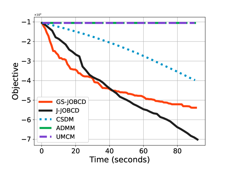
(a) Cifar(1000-100-50)

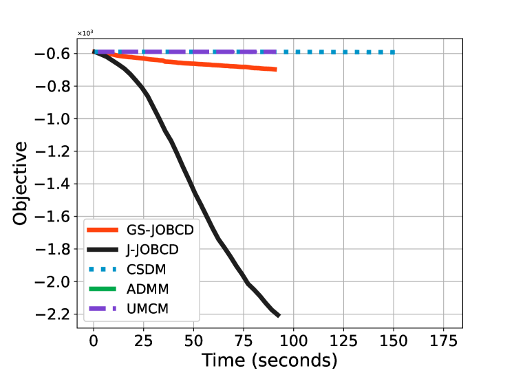
(b) CnnCaltech(2000-1000-500)

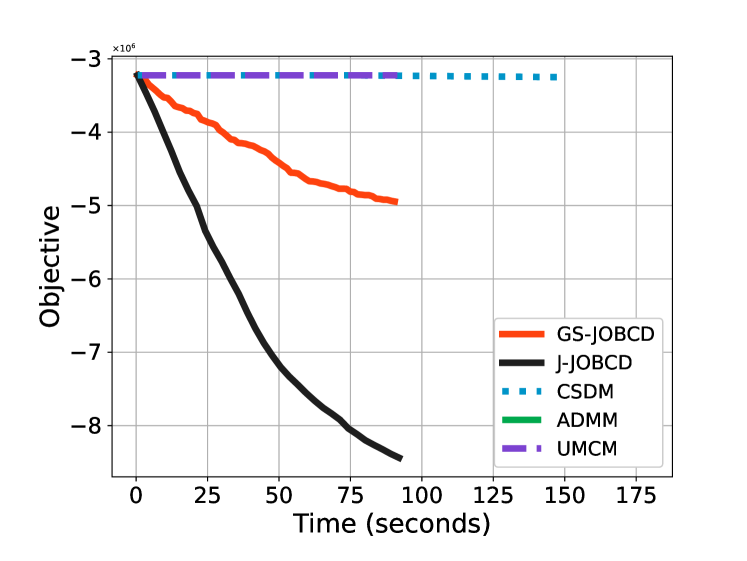
(c) gisette(3000-1000-500)

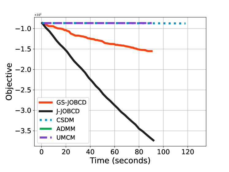
(d) mnist(1000-780-390)

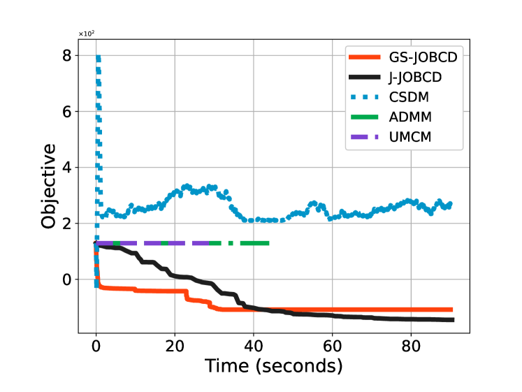
(e) randn(10-10-5)

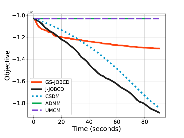
(f) randn(100-100-50)

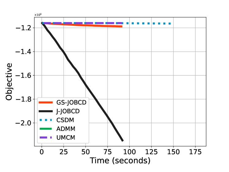
(g) randn(1000-1000-500)

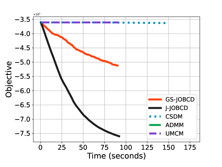
(h) sector(500-1000-500)

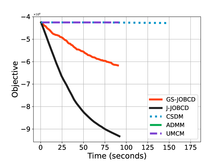
(i) TDT2(1000-1000-500)

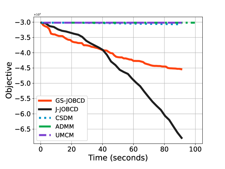
(j) w1a(2470-290-145)

Figure 3: The convergence curve of the compared methods for solving HEVP with varying $(m,n,p)$.

$\blacktriangleright$ Hyperbolic Eigenvalue Problem. Table 2 and Figure 3, 4, 5 are supplementary experiments for HEVP. Several conclusions can be drawn. (i) GS-JOBCD often greatly improves upon UMCM, ADMM and CSDM. This is because our methods find stronger stationary points than them. (ii) J-JOBCD is a parallel version of GS-JOBCD and thus exhibits significantly faster convergence. (iii) The proposed methods generally give the best performance.

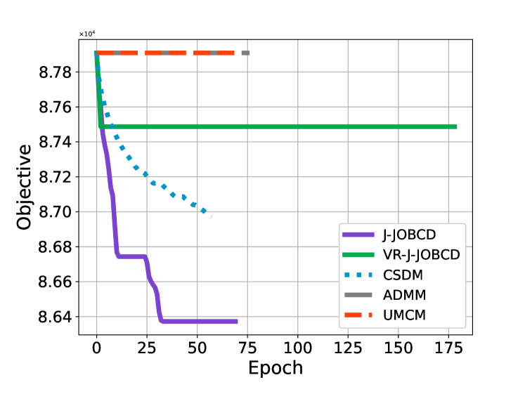
(a) 20News(9423-50-45)

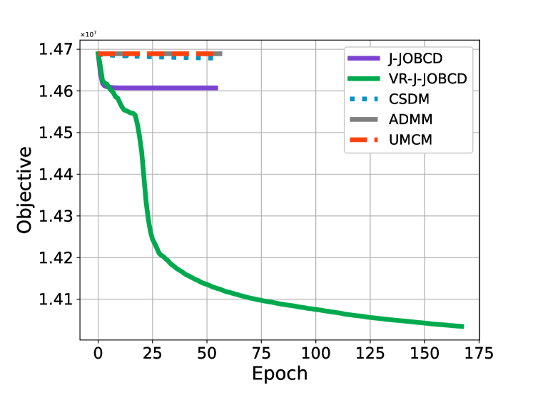
(b) Cifar(10000-50-45)

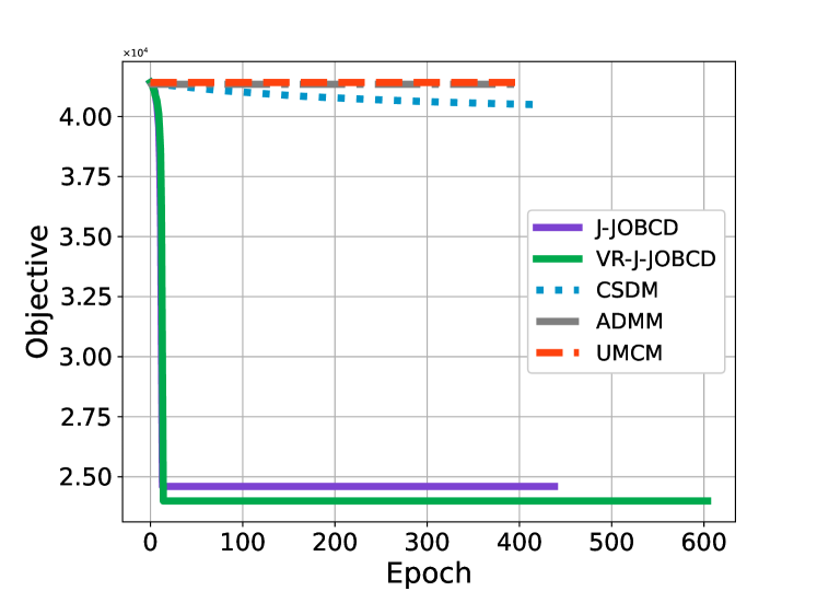
(c) CnnCaltech(3000-96-85)

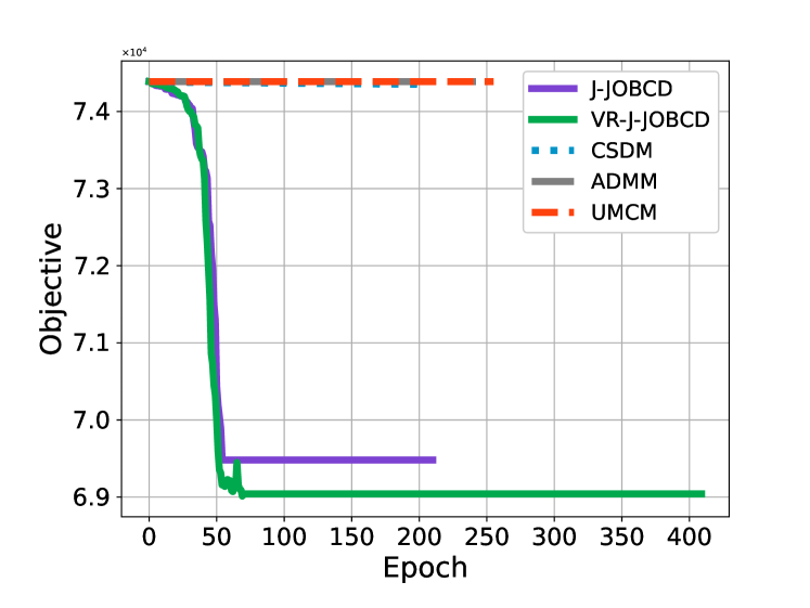
(d) E2006(5000-100-90)

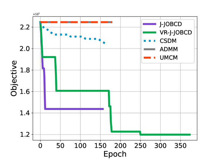
(e) Gisette(6000-50-45)

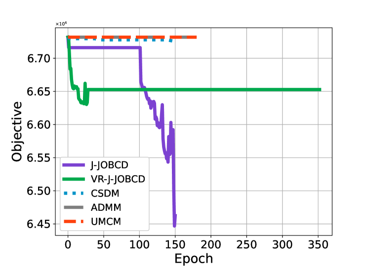
(f) Mnist(6000-92-85)

(g) News20(7967-50-45)

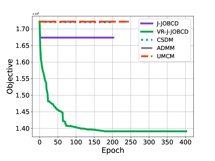
(h) randn(5000-100-85)

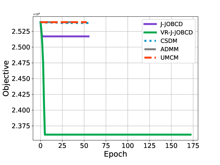
(i) randn(10000-50-45)

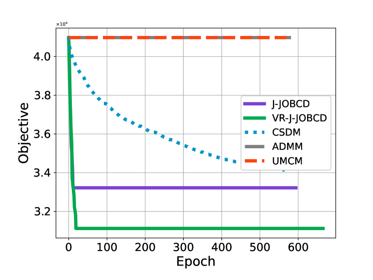
(j) W1a(2477-100-90)

Figure 6: The convergence curve of the compared methods for solving HSPP by epochs with varying $(m,n,p)$.

$\blacktriangleright$ Hyperbolic Structural Probe Problem. Table 3 and Figure 6, 7 are supplementary experiments for HSPP. Several conclusions can be drawn. (i) J-JOBCD often greatly improves upon UMCM, ADMM and CSDM (ii) VR-J-JOBCD is a reduced variance version of J-JOBCD and thus exhibits significantly faster convergence for problems with large samples. (iii) The proposed methods generally give the best performance.

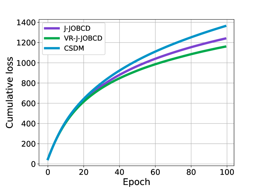
(a) Train accumulated loss

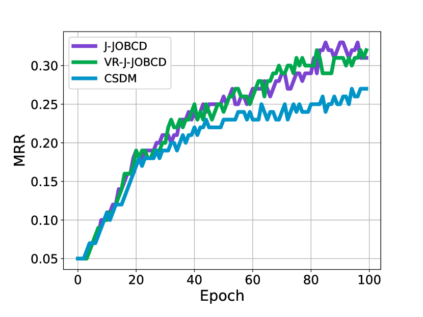
(b) Test MRR

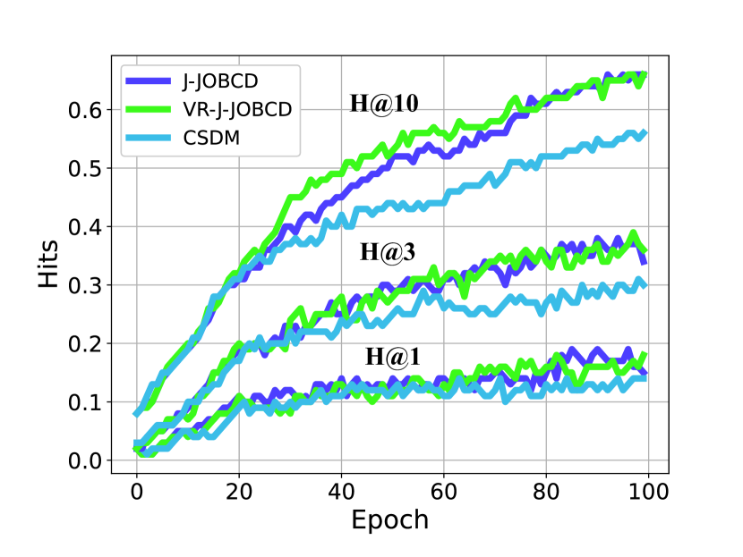
(c) Test Hits

Figure 8: Epoch performance of CS, J-JOBCD, and VR-J-JOBCD in training UltraE on FB15k.

$\blacktriangleright$ Ultra-hyperbolic Knowledge Graph Embedding Problem. Figure 8, 9, 10 and 11 are supplementary experiments for UltraE. Several conclusions can be drawn. (i) In terms of Epoch performance, J-JOBCD and VR-J-JOBCD often greatly improves upon CSDM, thus they show better MRR and hits results. (ii) In models with limited sample sizes, the computational efficiency of VR-J-JOBCD is inferior to that of J-JOBCD. This discrepancy arises because each iteration in VR-J-JOBCD necessitates two instances of backpropagation, thus consuming substantial computational resources. (iii) The proposed methods generally give the best performance.

F.3.1 Hyperbolic Eigenvalue Problem

Table 2: The convergence curve of the compared methods for solving HEVP. (+) indicates that after the convergence of the CSDM, UMCM and ADMM, utilizing the GS-JOBCD for optimization markedly enhances the objective value. The $1^{st},2^{\text{nd }}$, and $3^{\text{rd }}$ best results are colored with red, green and blue, respectively. $(n,p)$ represents the dimension and p-value of the J orthogonal matrix (square matrix). The value in $()$ stands for $\sum_{ij}^{n}|\mathbf{X}^{\top}\mathbf{J}\mathbf{X}-\mathbf{J}|_{ij}.$

dataname	(m-n-p)	UMCM	ADMM	CSDM	GS-JOBCD	J-JOBCD	UMCM+GS-JOBCD	ADMM+GS-JOBCD	CSDM+GS-JOBCD
time limit=30s
cifar	(1000-100-50)	-1.05e+04(3.0e-09)	-1.05e+04(3.0e-09)	-5.28e+04(4.8e-09)	-7.76e+04(1.6e-08)	-1.19e+05(8.1e-08)	-7.96e+04(1.1e-08)(+)	-5.86e+04(8.4e-09)(+)	-8.50e+04(1.2e-08)(+)
CnnCaltech	(2000-1000-500)	-5.89e+02(2.9e-08)	-5.89e+02(3.1e-10)	-7.86e+02(3.8e-10)	-7.68e+02(5.2e-10)	-3.90e+03(2.3e-08)	-6.71e+02(2.9e-08)(+)	-6.73e+02(3.6e-10)(+)	-8.49e+02(4.3e-10)(+)
gisette	(3000-1000-500)	-3.22e+06(3.1e-10)	-3.22e+06(3.1e-10)	-5.16e+06(3.9e-10)	-7.13e+06(5.9e-10)	-1.15e+07(1.5e-08)	-4.63e+06(3.7e-10)(+)	-4.74e+06(3.7e-10)(+)	-6.31e+06(4.6e-10)(+)
mnist	(1000-780-390)	-8.65e+04(4.1e-10)	-8.65e+04(4.1e-10)	-1.63e+05(4.9e-10)	-2.23e+05(6.6e-10)	-6.99e+05(2.1e-08)	-1.59e+05(4.7e-10)(+)	-1.48e+05(4.7e-10)(+)	-2.04e+05(5.7e-10)(+)
randn10	(10-10-5)	1.29e+02(9.7e-02)	1.29e+02(9.7e-02)	3.03e+02(2.3e-01)	-3.96e+01(9.7e-02)	-2.98e+02(9.7e-02)	-7.05e+01(9.7e-02)(+)	-1.75e+01(9.7e-02)(+)	2.29e+02(2.3e-01)(+)
randn100	(100-100-50)	-1.03e+04(3.0e-09)	-1.03e+04(2.5e-07)	-1.98e+04(5.1e-09)	-1.49e+04(2.7e-08)	-3.44e+04(1.3e-07)	-1.33e+04(1.4e-08)(+)	-1.31e+04(2.5e-07)(+)	-2.20e+04(1.8e-08)(+)
randn1000	(1000-1000-500)	-1.16e+06(3.1e-10)	-1.16e+06(3.1e-10)	-1.47e+06(3.9e-10)	-1.20e+06(4.4e-10)	-4.83e+06(7.3e-08)	-1.18e+06(3.5e-10)(+)	-1.18e+06(3.5e-10)(+)	-1.49e+06(4.7e-10)(+)
sector	(500-1000-500)	-3.61e+03(3.1e-10)	-3.61e+03(3.1e-10)	-5.35e+03(3.9e-10)	-6.68e+03(5.8e-10)	-1.07e+04(1.2e-08)	-4.73e+03(3.7e-10)(+)	-4.85e+03(3.6e-10)(+)	-6.47e+03(4.6e-10)(+)
TDT2	(1000-1000-500)	-4.25e+06(3.1e-10)	-4.25e+06(3.1e-10)	-6.37e+06(4.0e-10)	-8.20e+06(6.0e-10)	-1.32e+07(1.2e-08)	-5.67e+06(3.7e-10)(+)	-5.93e+06(3.7e-10)(+)	-7.85e+06(4.8e-10)(+)
w1a	(2470-290-145)	-3.02e+04(1.1e-04)	-3.02e+04(1.1e-04)	-5.42e+04(4.4e-04)	-5.74e+04(1.1e-04)	-6.73e+05(1.1e-04)	-4.76e+04(1.1e-04)(+)	-4.57e+04(1.1e-04)(+)	-6.32e+04(4.4e-04)(+)
cifar	(1000-100-70)	-7.32e+03(1.9e-09)	-7.32e+03(1.9e-09)	-3.29e+04(3.2e-09)	-6.01e+04(1.5e-08)	-1.12e+05(7.4e-08)	-4.84e+04(1.0e-08)(+)	-4.30e+04(7.6e-09)(+)	-7.52e+04(1.3e-08)(+)
CnnCaltech	(2000-1000-700)	-4.33e+02(2.1e-08)	-4.33e+02(2.2e-10)	-5.43e+02(2.5e-10)	-5.69e+02(3.6e-10)	-2.88e+03(1.6e-08)	-4.86e+02(2.1e-08)(+)	-4.85e+02(2.6e-10)(+)	-5.98e+02(3.0e-10)(+)
gisette	(1000,700)	-2.45e+06(2.2e-10)	-2.45e+06(2.2e-10)	-3.59e+06(2.5e-10)	-5.02e+06(4.2e-10)	-9.17e+06(1.0e-08)	-3.15e+06(2.5e-10)(+)	-3.25e+06(2.5e-10)(+)	-4.25e+06(2.7e-10)(+)
mnist	(1000-780-500)	-7.05e+04(3.1e-10)	-7.05e+04(3.1e-10)	-1.21e+05(3.6e-10)	-1.81e+05(5.3e-10)	-6.28e+05(1.9e-08)	-1.14e+05(3.5e-10)(+)	-1.21e+05(3.6e-10)(+)	-1.59e+05(4.3e-10)(+)
randn10	(10-10-7)	1.61e+02(5.6e-02)	1.61e+02(5.6e-02)	3.46e+02(1.8e-01)	-4.14e+11(2.1e+02)	-1.64e+00(5.6e-02)	3.69e+01(5.6e-02)(+)	-8.63e+02(5.6e-02)(+)	2.96e+02(1.8e-01)(+)
randn100	(100,70)	-8.00e+03(1.9e-09)	-8.00e+03(1.8e-07)	-1.41e+04(2.9e-09)	-1.10e+04(1.9e-08)	-2.37e+04(8.5e-08)	-9.68e+03(9.3e-09)(+)	-9.75e+03(1.8e-07)(+)	-1.64e+04(1.3e-08)(+)
randn1000	(1000-1000-700)	-8.88e+05(2.2e-10)	-8.88e+05(2.2e-10)	-1.07e+06(2.7e-10)	-9.15e+05(3.4e-10)	-3.24e+06(4.3e-08)	-9.04e+05(2.6e-10)(+)	-9.05e+05(2.5e-10)(+)	-1.09e+06(3.2e-10)(+)
sector	(500-1000-700)	-2.66e+03(2.2e-10)	-2.66e+03(2.2e-10)	-3.63e+03(2.5e-10)	-4.57e+03(3.8e-10)	-8.93e+03(9.1e-09)	-3.16e+03(2.4e-10)(+)	-3.26e+03(2.4e-10)(+)	-4.12e+03(2.8e-10)(+)
TDT2	(1000-1000-700)	-3.15e+06(2.2e-10)	-3.15e+06(2.2e-10)	-4.33e+06(2.5e-10)	-5.32e+06(3.4e-10)	-1.23e+07(9.1e-09)	-3.80e+06(2.5e-10)(+)	-3.75e+06(2.4e-10)(+)	-4.77e+06(2.8e-10)(+)
w1a	(2470-290-200)	-2.77e+04(8.0e-10)	-2.77e+04(8.0e-10)	-3.93e+04(1.1e-09)	-5.19e+04(4.1e-09)	-3.97e+05(5.6e-08)	-4.05e+04(1.8e-09)(+)	-3.73e+04(1.7e-09)(+)	-5.45e+04(2.9e-09)(+)
cifar	(1000-100-90)	-6.42e+03(1.2e-09)	-6.42e+03(1.2e-09)	-1.59e+04(1.2e-09)	-4.51e+04(1.4e-08)	-5.05e+04(5.6e-08)	-2.64e+04(6.3e-09)(+)	-3.35e+04(7.0e-09)(+)	-3.89e+04(6.7e-09)(+)
CnnCaltech	(2000-1000-900)	-3.10e+02(1.1e-08)	-3.10e+02(1.2e-10)	-3.41e+02(1.3e-10)	-3.64e+02(1.7e-10)	-1.65e+03(8.0e-09)	-3.29e+02(1.1e-08)(+)	-3.32e+02(1.3e-10)(+)	-3.61e+02(1.4e-10)(+)
gisette	(3000-1000-900)	-1.74e+06(1.2e-10)	-1.74e+06(1.2e-10)	-2.05e+06(1.2e-10)	-2.57e+06(1.8e-10)	-6.46e+06(8.0e-09)	-2.00e+06(1.3e-10)(+)	-1.99e+06(1.2e-10)(+)	-2.33e+06(1.4e-10)(+)
mnist	(1000-780-650)	-5.19e+04(1.9e-10)	-5.19e+04(1.9e-10)	-6.12e+04(2.2e-10)	-1.02e+05(2.9e-10)	-4.03e+05(1.2e-08)	-6.75e+04(2.1e-10)(+)	-6.58e+04(2.1e-10)(+)	-7.54e+04(2.4e-10)(+)
randn10	(10-10-9)	5.33e+02(1.7e-01)	5.33e+02(1.7e-01)	4.28e+02(1.3e-01)	-1.03e+12(5.5e+02)	3.64e+02(1.7e-01)	2.21e+02(1.7e-01)(+)	-3.46e+02(1.7e-01)(+)	1.54e+02(1.3e-01)(+)
randn100	(100-100-90)	-6.14e+03(1.1e-07)	-6.14e+03(1.2e-09)	-8.14e+03(1.4e-09)	-8.31e+03(1.5e-08)	-1.31e+04(5.8e-08)	-7.74e+03(1.2e-07)(+)	-7.77e+03(1.3e-08)(+)	-9.69e+03(1.1e-08)(+)
randn1000	(1000-1000-900)	-6.33e+05(1.2e-10)	-6.33e+05(1.2e-10)	-6.84e+05(1.3e-10)	-6.46e+05(1.9e-10)	-1.87e+06(1.8e-08)	-6.39e+05(1.3e-10)(+)	-6.39e+05(1.3e-10)(+)	-6.90e+05(1.5e-10)(+)
sector	(500-1000-900)	-1.92e+03(1.2e-10)	-1.92e+03(1.2e-10)	-2.18e+03(1.2e-10)	-2.50e+03(1.6e-10)	-5.84e+03(6.5e-09)	-2.12e+03(1.2e-10)(+)	-2.13e+03(1.2e-10)(+)	-2.34e+03(1.4e-10)(+)
TDT2	(1000-1000-900)	-2.26e+06(1.2e-10)	-2.26e+06(1.2e-10)	-2.58e+06(1.2e-10)	-2.90e+06(1.6e-10)	-7.40e+06(6.6e-09)	-2.53e+06(1.2e-10)(+)	-2.51e+06(1.2e-10)(+)	-2.83e+06(1.3e-10)(+)
w1a	(2470-290-250)	-2.03e+04(5.4e-10)	-2.03e+04(5.4e-10)	-2.41e+04(5.9e-10)	-3.74e+04(2.9e-09)	-2.59e+05(3.3e-08)	-2.82e+04(1.2e-09)(+)	-3.17e+04(1.4e-09)(+)	-3.78e+04(1.5e-09)(+)
time limit=60s
cifar	(1000-100-50)	-1.05e+04(3.0e-09)	-1.05e+04(3.0e-09)	-5.28e+04(4.7e-09)	-9.03e+04(2.2e-08)	-1.14e+05(1.1e-07)	-8.07e+04(1.5e-08)(+)	-6.87e+04(1.3e-08)(+)	-1.01e+05(1.6e-08)(+)
CnnCaltech	(2000-1000-500)	-5.89e+02(2.9e-08)	-5.89e+02(3.1e-10)	-9.79e+02(4.6e-10)	-9.58e+02(9.9e-10)	-6.68e+03(4.7e-08)	-7.13e+02(2.9e-08)(+)	-7.23e+02(4.3e-10)(+)	-1.05e+03(5.9e-10)(+)
gisette	(3000-1000-500)	-3.22e+06(3.1e-10)	-3.22e+06(3.1e-10)	-6.54e+06(4.3e-10)	-8.84e+06(9.7e-10)	-1.29e+07(2.1e-08)	-5.55e+06(4.1e-10)(+)	-5.67e+06(4.2e-10)(+)	-8.02e+06(6.4e-10)(+)
mnist	(1000-780-390)	-8.65e+04(4.1e-10)	-8.65e+04(4.1e-10)	-2.28e+05(5.3e-10)	-2.75e+05(9.5e-10)	-9.32e+05(3.2e-08)	-1.80e+05(5.4e-10)(+)	-1.88e+05(5.4e-10)(+)	-2.83e+05(6.8e-10)(+)
randn10	(10-10-5)	1.29e+02(9.7e-02)	1.29e+02(9.7e-02)	2.43e+02(2.2e-01)	-3.96e+01(9.7e-02)	-7.07e+01(9.7e-02)	-2.27e+05(9.7e-02)(+)	-3.46e+02(9.7e-02)(+)	-2.94e+05(2.2e-01)(+)
randn100	(100-100-50)	-1.03e+04(3.0e-09)	-1.03e+04(2.5e-07)	-1.98e+04(5.4e-09)	-1.81e+04(4.3e-08)	-3.88e+04(1.9e-07)	-1.41e+04(1.9e-08)(+)	-1.44e+04(2.5e-07)(+)	-2.41e+04(2.9e-08)(+)
randn1000	(1000-1000-500)	-1.16e+06(3.1e-10)	-1.16e+06(3.1e-10)	-1.79e+06(4.7e-10)	-1.21e+06(6.0e-10)	-7.79e+06(1.5e-07)	-1.19e+06(3.9e-10)(+)	-1.19e+06(4.0e-10)(+)	-1.81e+06(5.7e-10)(+)
sector	(500-1000-500)	-3.61e+03(3.1e-10)	-3.61e+03(3.1e-10)	-6.63e+03(4.5e-10)	-8.22e+03(9.1e-10)	-1.11e+04(1.7e-08)	-5.53e+03(4.2e-10)(+)	-5.63e+03(4.3e-10)(+)	-7.83e+03(5.8e-10)(+)
TDT2	(1000-1000-500)	-4.25e+06(3.1e-10)	-4.25e+06(3.1e-10)	-8.31e+06(4.4e-10)	-9.87e+06(8.9e-10)	-1.43e+07(1.7e-08)	-6.51e+06(4.1e-10)(+)	-6.80e+06(4.2e-10)(+)	-9.33e+06(5.3e-10)(+)
w1a	(2470-290-145)	-3.02e+04(1.1e-04)	-3.02e+04(1.1e-04)	-5.63e+04(1.0e-04)	-7.13e+04(1.1e-04)	-2.07e+06(1.1e-04)	-5.44e+04(1.1e-04)(+)	-5.42e+04(1.1e-04)(+)	-6.91e+04(1.0e-04)(+)
cifar	(1000-100-70)	-7.32e+03(1.9e-09)	-7.32e+03(1.9e-09)	-3.29e+04(3.3e-09)	-6.94e+04(1.9e-08)	-9.31e+04(9.6e-08)	-5.69e+04(1.4e-08)(+)	-5.87e+04(1.4e-08)(+)	-8.58e+04(1.8e-08)(+)
CnnCaltech	(2000-1000-700)	-4.33e+02(2.1e-08)	-4.33e+02(2.2e-10)	-6.99e+02(3.2e-10)	-6.74e+02(5.7e-10)	-4.74e+03(3.1e-08)	-5.23e+02(2.1e-08)(+)	-5.21e+02(2.7e-10)(+)	-7.62e+02(4.1e-10)(+)
gisette	(1000,700)	-2.45e+06(2.2e-10)	-2.45e+06(2.2e-10)	-4.99e+06(2.8e-10)	-6.15e+06(6.0e-10)	-1.15e+07(1.6e-08)	-3.71e+06(2.6e-10)(+)	-3.86e+06(2.7e-10)(+)	-5.81e+06(3.7e-10)(+)
mnist	(1000-780-500)	-7.05e+04(3.1e-10)	-7.05e+04(3.1e-10)	-1.62e+05(4.3e-10)	-2.19e+05(6.8e-10)	-8.50e+05(2.6e-08)	-1.34e+05(4.0e-10)(+)	-1.41e+05(3.9e-10)(+)	-2.00e+05(5.1e-10)(+)
randn10	(10-10-7)	1.61e+02(5.6e-02)	1.61e+02(5.6e-02)	3.81e+02(1.6e-01)	-3.45e+16(9.0e+06)	4.37e-01(5.6e-02)	-2.19e+04(5.6e-02)(+)	-2.03e+04(5.6e-02)(+)	3.39e+02(1.6e-01)(+)
randn100	(100,70)	-8.00e+03(1.9e-09)	-8.00e+03(1.8e-07)	-1.41e+04(2.9e-09)	-1.37e+04(3.2e-08)	-2.69e+04(1.4e-07)	-1.04e+04(1.3e-08)(+)	-1.08e+04(1.8e-07)(+)	-1.83e+04(2.7e-08)(+)
randn1000	(1000-1000-700)	-8.88e+05(2.2e-10)	-8.88e+05(2.2e-10)	-1.31e+06(3.0e-10)	-9.25e+05(4.5e-10)	-5.49e+06(9.7e-08)	-9.09e+05(2.8e-10)(+)	-9.09e+05(2.7e-10)(+)	-1.33e+06(3.8e-10)(+)
sector	(500-1000-700)	-2.66e+03(2.2e-10)	-2.66e+03(2.2e-10)	-5.05e+03(3.0e-10)	-5.74e+03(5.6e-10)	-1.13e+04(1.4e-08)	-3.74e+03(2.7e-10)(+)	-3.74e+03(2.7e-10)(+)	-5.65e+03(4.0e-10)(+)
TDT2	(1000-1000-700)	-3.15e+06(2.2e-10)	-3.15e+06(2.2e-10)	-6.13e+06(3.1e-10)	-6.94e+06(5.7e-10)	-1.45e+07(1.4e-08)	-4.55e+06(2.7e-10)(+)	-4.54e+06(2.8e-10)(+)	-6.99e+06(4.1e-10)(+)
w1a	(2470-290-200)	-2.77e+04(8.0e-10)	-2.77e+04(8.0e-10)	-4.00e+04(1.1e-09)	-7.13e+04(1.2e-08)	-3.42e+06(5.3e-07)	-4.71e+04(3.6e-09)(+)	-5.28e+04(4.3e-09)(+)	-6.55e+04(5.1e-09)(+)
cifar	(1000-100-90)	-6.42e+03(1.2e-09)	-6.42e+03(1.2e-09)	-1.60e+04(1.5e-09)	-4.91e+04(2.0e-08)	-4.97e+04(9.3e-08)	-4.12e+04(1.2e-08)(+)	-4.83e+04(1.6e-08)(+)	-4.87e+04(1.7e-08)(+)
CnnCaltech	(2000-1000-900)	-3.10e+02(1.1e-08)	-3.10e+02(1.2e-10)	-3.15e+02(1.2e-10)	-4.25e+02(3.1e-10)	-2.37e+03(1.4e-08)	-3.44e+02(1.1e-08)(+)	-3.41e+02(1.4e-10)(+)	-3.45e+02(1.4e-10)(+)
gisette	(3000-1000-900)	-1.74e+06(1.2e-10)	-1.74e+06(1.2e-10)	-2.59e+06(1.4e-10)	-3.09e+06(2.6e-10)	-8.40e+06(1.2e-08)	-2.21e+06(1.3e-10)(+)	-2.19e+06(1.3e-10)(+)	-2.79e+06(1.7e-10)(+)
mnist	(1000-780-650)	-5.19e+04(1.9e-10)	-5.19e+04(1.9e-10)	-6.81e+04(2.4e-10)	-1.35e+05(4.4e-10)	-5.92e+05(2.0e-08)	-7.34e+04(2.2e-10)(+)	-7.07e+04(2.3e-10)(+)	-9.21e+04(2.8e-10)(+)
randn10	(10-10-9)	5.33e+02(1.7e-01)	5.33e+02(1.7e-01)	5.07e+02(2.3e-01)	-1.28e+19(4.2e+09)	3.41e+02(1.7e-01)	-2.71e+04(1.7e-01)(+)	4.49e+02(1.7e-01)(+)	2.41e+02(2.3e-01)(+)
randn100	(100-100-90)	-6.14e+03(1.1e-07)	-6.14e+03(1.2e-09)	-8.14e+03(1.7e-09)	-1.08e+04(2.6e-08)	-1.56e+04(9.7e-08)	-8.18e+03(1.2e-07)(+)	-8.15e+03(1.2e-08)(+)	-1.12e+04(2.1e-08)(+)
randn1000	(1000-1000-900)	-6.33e+05(1.2e-10)	-6.33e+05(1.2e-10)	-7.65e+05(1.5e-10)	-6.49e+05(2.4e-10)	-2.77e+06(3.5e-08)	-6.42e+05(1.4e-10)(+)	-6.41e+05(1.4e-10)(+)	-7.72e+05(1.8e-10)(+)
sector	(500-1000-900)	-1.92e+03(1.2e-10)	-1.92e+03(1.2e-10)	-2.66e+03(1.4e-10)	-2.80e+03(2.1e-10)	-7.48e+03(1.1e-08)	-2.23e+03(1.3e-10)(+)	-2.32e+03(1.4e-10)(+)	-2.82e+03(1.7e-10)(+)
TDT2	(1000-1000-900)	-2.26e+06(1.2e-10)	-2.26e+06(1.2e-10)	-3.18e+06(1.4e-10)	-3.33e+06(2.0e-10)	-8.81e+06(9.7e-09)	-2.72e+06(1.4e-10)(+)	-2.73e+06(1.3e-10)(+)	-3.37e+06(1.7e-10)(+)
w1a	(2470-290-250)	-2.03e+04(5.4e-10)	-2.03e+04(5.4e-10)	-2.42e+04(7.0e-10)	-4.96e+04(7.1e-09)	-1.56e+06(2.5e-07)	-3.55e+04(3.2e-09)(+)	-3.67e+04(2.9e-09)(+)	-4.36e+04(2.8e-09)(+)
time limit=90s
cifar	(1000-100-50)	-1.05e+04(3.0e-09)	-1.05e+04(3.0e-09)	-5.28e+04(5.4e-09)	-1.03e+05(2.6e-08)	-1.11e+05(1.4e-07)	-8.38e+04(1.7e-08)(+)	-8.39e+04(1.9e-08)(+)	-1.24e+05(2.6e-08)(+)
CnnCaltech	(2000-1000-500)	-5.89e+02(2.9e-08)	-5.89e+02(3.1e-10)	-1.11e+03(5.2e-10)	-1.07e+03(1.3e-09)	-9.16e+03(6.9e-08)	-7.44e+02(2.9e-08)(+)	-7.51e+02(4.6e-10)(+)	-1.15e+03(6.9e-10)(+)
gisette	(3000-1000-500)	-3.22e+06(3.1e-10)	-3.22e+06(3.1e-10)	-8.53e+06(4.9e-10)	-9.49e+06(1.2e-09)	-1.36e+07(2.6e-08)	-6.21e+06(4.6e-10)(+)	-6.23e+06(4.9e-10)(+)	-9.65e+06(7.9e-10)(+)
mnist	(1000-780-390)	-8.65e+04(4.1e-10)	-8.65e+04(4.1e-10)	-2.56e+05(5.6e-10)	-3.14e+05(1.2e-09)	-1.20e+06(4.1e-08)	-2.05e+05(5.8e-10)(+)	-2.11e+05(6.1e-10)(+)	-3.06e+05(7.6e-10)(+)
randn10	(10-10-5)	1.29e+02(9.7e-02)	1.29e+02(9.7e-02)	2.45e+02(2.3e-01)	-3.96e+01(9.7e-02)	-3.97e+02(9.7e-02)	1.17e+01(9.7e-02)(+)	-2.66e+09(1.1e+00)(+)	1.55e+01(2.3e-01)(+)
randn100	(100-100-50)	-1.03e+04(3.0e-09)	-1.03e+04(2.5e-07)	-1.98e+04(4.4e-09)	-2.28e+04(5.6e-08)	-4.37e+04(2.6e-07)	-1.50e+04(2.5e-08)(+)	-1.54e+04(2.6e-07)(+)	-2.41e+04(4.2e-08)(+)
randn1000	(1000-1000-500)	-1.16e+06(3.1e-10)	-1.16e+06(3.1e-10)	-1.93e+06(5.0e-10)	-1.22e+06(6.9e-10)	-1.04e+07(2.3e-07)	-1.19e+06(4.1e-10)(+)	-1.19e+06(4.4e-10)(+)	-1.95e+06(6.7e-10)(+)
sector	(500-1000-500)	-3.61e+03(3.1e-10)	-3.61e+03(3.1e-10)	-7.90e+03(4.9e-10)	-9.24e+03(1.3e-09)	-1.06e+04(2.0e-08)	-5.56e+03(4.3e-10)(+)	-5.69e+03(4.3e-10)(+)	-8.51e+03(6.4e-10)(+)
TDT2	(1000-1000-500)	-4.25e+06(3.1e-10)	-4.25e+06(3.1e-10)	-9.39e+06(4.8e-10)	-1.05e+07(1.1e-09)	-1.42e+07(2.1e-08)	-6.65e+06(4.4e-10)(+)	-6.89e+06(4.2e-10)(+)	-1.04e+07(6.5e-10)(+)
w1a	(2470-290-145)	-3.02e+04(1.1e-04)	-3.02e+04(1.1e-04)	-5.72e+04(2.7e-05)	-9.21e+04(1.1e-04)	-9.32e+06(1.1e-04)	-5.74e+04(1.1e-04)(+)	-6.40e+04(1.1e-04)(+)	-7.94e+04(2.7e-05)(+)
cifar	(1000-100-70)	-7.32e+03(1.9e-09)	-7.32e+03(1.9e-09)	-3.29e+04(3.1e-09)	-7.19e+04(2.1e-08)	-1.36e+05(1.2e-07)	-6.05e+04(1.8e-08)(+)	-6.42e+04(1.8e-08)(+)	-9.76e+04(2.5e-08)(+)
CnnCaltech	(2000-1000-700)	-4.33e+02(2.1e-08)	-4.33e+02(2.2e-10)	-7.42e+02(3.1e-10)	-7.76e+02(8.4e-10)	-6.63e+03(4.7e-08)	-5.23e+02(2.1e-08)(+)	-5.38e+02(3.0e-10)(+)	-8.08e+02(4.2e-10)(+)
gisette	(1000,700)	-2.45e+06(2.2e-10)	-2.45e+06(2.2e-10)	-5.56e+06(3.1e-10)	-6.76e+06(7.5e-10)	-1.13e+07(1.9e-08)	-3.90e+06(3.0e-10)(+)	-4.02e+06(3.0e-10)(+)	-6.62e+06(4.4e-10)(+)
mnist	(1000-780-500)	-7.05e+04(3.1e-10)	-7.05e+04(3.1e-10)	-1.71e+05(4.5e-10)	-2.51e+05(8.4e-10)	-1.09e+06(3.5e-08)	-1.58e+05(4.3e-10)(+)	-1.46e+05(4.4e-10)(+)	-2.23e+05(5.9e-10)(+)
randn10	(10-10-7)	1.61e+02(5.6e-02)	1.61e+02(5.6e-02)	3.33e+02(1.7e-01)	6.45e+01(5.6e-02)	5.58e+01(5.6e-02)	1.15e+02(5.6e-02)(+)	8.86e+01(5.6e-02)(+)	1.67e+02(1.7e-01)(+)
randn100	(100,70)	-8.00e+03(1.9e-09)	-8.00e+03(1.8e-07)	-1.41e+04(3.0e-09)	-1.43e+04(3.0e-08)	-2.60e+04(1.7e-07)	-1.05e+04(1.4e-08)(+)	-1.08e+04(1.8e-07)(+)	-1.87e+04(3.2e-08)(+)
randn1000	(1000-1000-700)	-8.88e+05(2.2e-10)	-8.88e+05(2.2e-10)	-1.36e+06(3.1e-10)	-9.25e+05(4.6e-10)	-7.05e+06(1.4e-07)	-9.10e+05(2.8e-10)(+)	-9.10e+05(2.8e-10)(+)	-1.37e+06(4.2e-10)(+)
sector	(500-1000-700)	-2.66e+03(2.2e-10)	-2.66e+03(2.2e-10)	-5.64e+03(3.2e-10)	-5.40e+03(5.2e-10)	-1.53e+04(1.8e-08)	-3.67e+03(2.6e-10)(+)	-3.80e+03(2.8e-10)(+)	-5.94e+03(4.0e-10)(+)
TDT2	(1000-1000-700)	-3.15e+06(2.2e-10)	-3.15e+06(2.2e-10)	-6.78e+06(3.2e-10)	-6.43e+06(5.0e-10)	-1.33e+07(1.6e-08)	-4.49e+06(2.9e-10)(+)	-4.51e+06(2.6e-10)(+)	-7.19e+06(4.2e-10)(+)
w1a	(2470-290-200)	-2.77e+04(8.0e-10)	-2.77e+04(8.0e-10)	-4.00e+04(1.1e-09)	-7.60e+04(1.2e-08)	-8.13e+06(1.3e-06)	-5.33e+04(4.8e-09)(+)	-5.40e+04(4.5e-09)(+)	-6.47e+04(5.6e-09)(+)
cifar	(1000-100-90)	-6.42e+03(1.2e-09)	-6.42e+03(1.2e-09)	-1.60e+04(1.3e-09)	-3.78e+04(1.3e-08)	-5.24e+04(1.2e-07)	-2.77e+04(6.1e-09)(+)	-2.53e+04(4.8e-09)(+)	-3.60e+04(7.8e-09)(+)
CnnCaltech	(2000-1000-900)	-3.10e+02(1.1e-08)	-3.10e+02(1.2e-10)	-4.05e+02(1.6e-10)	-3.99e+02(2.6e-10)	-3.16e+03(2.0e-08)	-3.45e+02(1.1e-08)(+)	-3.42e+02(1.4e-10)(+)	-4.36e+02(2.0e-10)(+)
gisette	(3000-1000-900)	-1.74e+06(1.2e-10)	-1.74e+06(1.2e-10)	-2.84e+06(1.4e-10)	-2.76e+06(1.9e-10)	-9.30e+06(1.6e-08)	-2.16e+06(1.3e-10)(+)	-2.15e+06(1.3e-10)(+)	-3.06e+06(1.6e-10)(+)
mnist	(1000-780-650)	-5.19e+04(1.9e-10)	-5.19e+04(1.9e-10)	-6.85e+04(2.4e-10)	-1.28e+05(4.0e-10)	-7.18e+05(2.5e-08)	-8.43e+04(2.3e-10)(+)	-8.21e+04(2.3e-10)(+)	-1.06e+05(2.7e-10)(+)
randn10	(10-10-9)	5.33e+02(1.7e-01)	5.33e+02(1.7e-01)	4.54e+02(2.1e-01)	-2.28e+05(1.7e-01)	4.62e+02(1.7e-01)	1.80e+01(1.7e-01)(+)	-6.43e+00(1.7e-01)(+)	-1.06e+02(2.1e-01)(+)
randn100	(100-100-90)	-6.14e+03(1.1e-07)	-6.14e+03(1.2e-09)	-8.14e+03(1.5e-09)	-1.12e+04(2.5e-08)	-1.36e+04(1.2e-07)	-8.09e+03(1.2e-07)(+)	-8.48e+03(1.7e-08)(+)	-1.11e+04(2.1e-08)(+)
randn1000	(1000-1000-900)	-6.33e+05(1.2e-10)	-6.33e+05(1.2e-10)	-7.87e+05(1.5e-10)	-6.50e+05(2.5e-10)	-3.36e+06(4.5e-08)	-6.42e+05(1.5e-10)(+)	-6.44e+05(1.5e-10)(+)	-7.94e+05(2.0e-10)(+)
sector	(500-1000-900)	-1.92e+03(1.2e-10)	-1.92e+03(1.2e-10)	-2.89e+03(1.5e-10)	-2.80e+03(1.9e-10)	-8.81e+03(1.3e-08)	-2.26e+03(1.3e-10)(+)	-2.30e+03(1.3e-10)(+)	-2.99e+03(1.7e-10)(+)
TDT2	(1000-1000-900)	-2.26e+06(1.2e-10)	-2.26e+06(1.2e-10)	-3.46e+06(1.5e-10)	-3.38e+06(2.0e-10)	-1.29e+07(1.4e-08)	-2.73e+06(1.3e-10)(+)	-2.65e+06(1.3e-10)(+)	-3.57e+06(1.7e-10)(+)
w1a	(2470-290-250)	-2.03e+04(5.4e-10)	-2.03e+04(5.4e-10)	-2.42e+04(6.2e-10)	-5.60e+04(8.5e-09)	-9.37e+06(1.1e-06)	-3.95e+04(3.5e-09)(+)	-3.90e+04(3.5e-09)(+)	-5.02e+04(3.4e-09)(+)

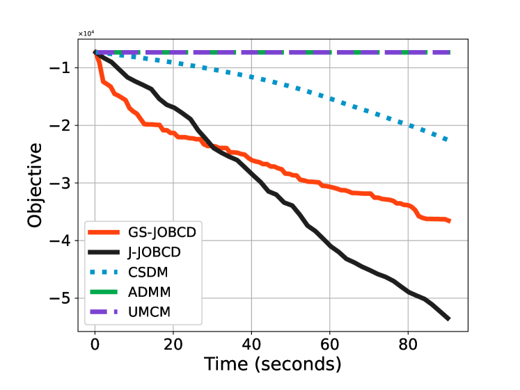
(a) Cifar(1000-100-70)

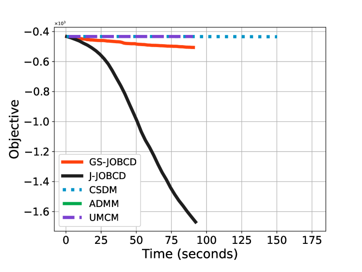
(b) CnnCaltech(2000-1000-700)

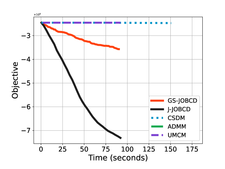
(c) gisette(3000-1000-700)

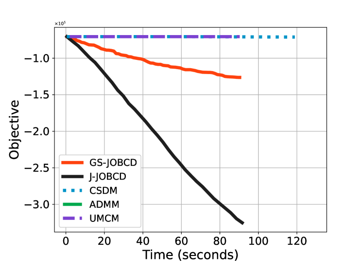
(d) mnist(1000-780-500)

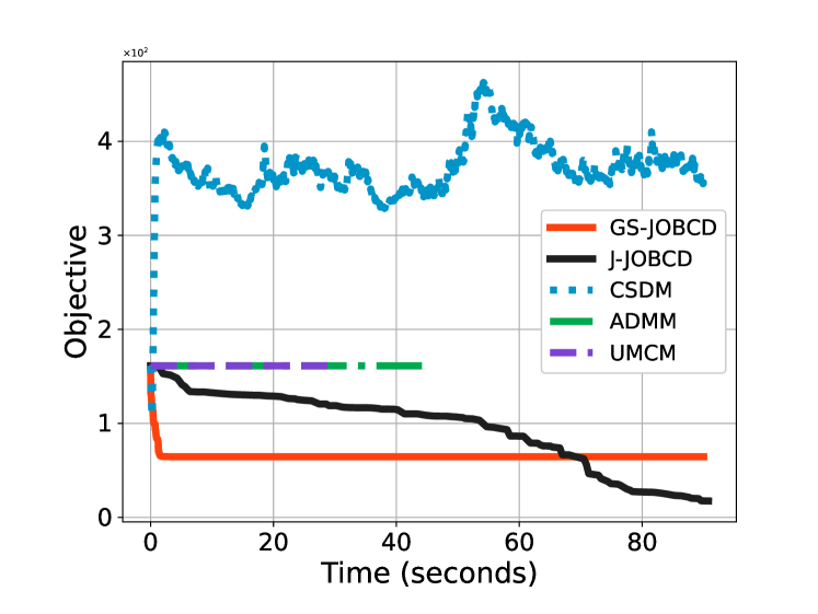
(e) randn(10-10-7)

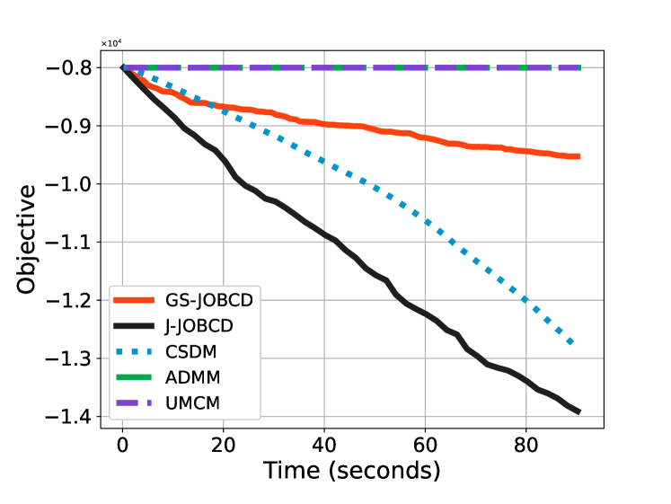
(f) randn(100-100-70)

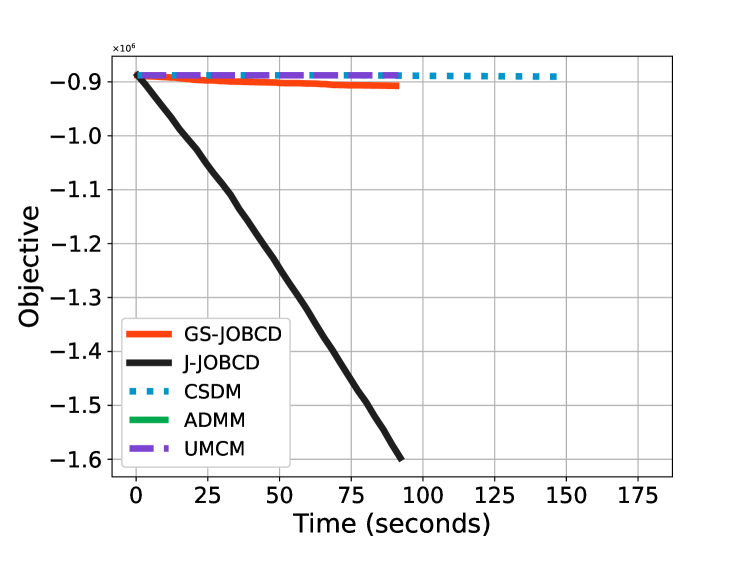
(g) randn(1000-1000-700)

(h) sector(500-1000-700)

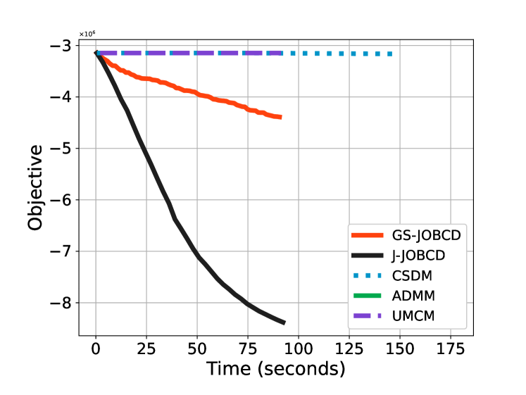
(i) TDT2(1000-1000-700)

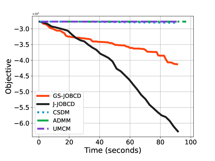
(j) w1a(2470-290-200)

Figure 4: The convergence curve of the compared methods for solving HEVP with varying $(m,n,p)$.

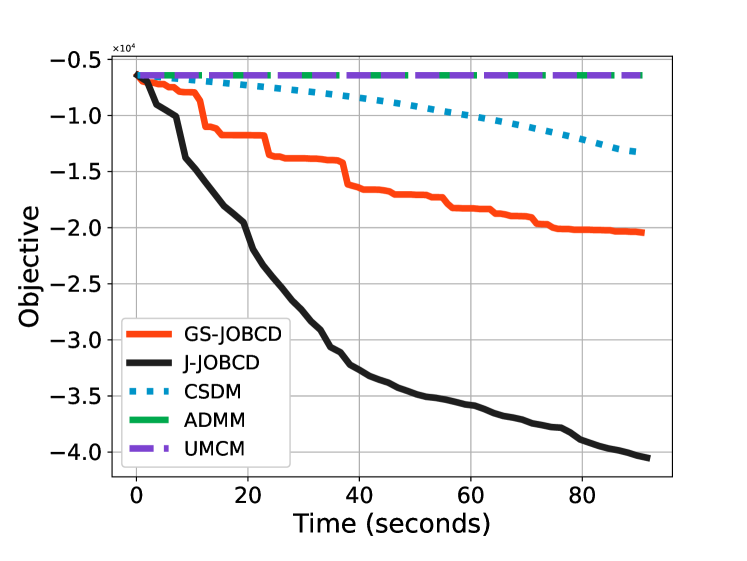
(a) Cifar(1000-100-90)

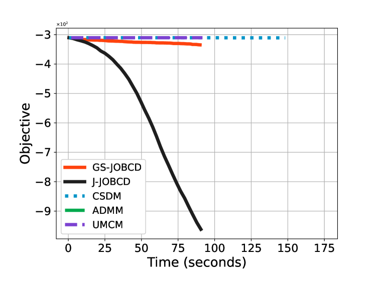
(b) CnnCaltech(2000-1000-900)

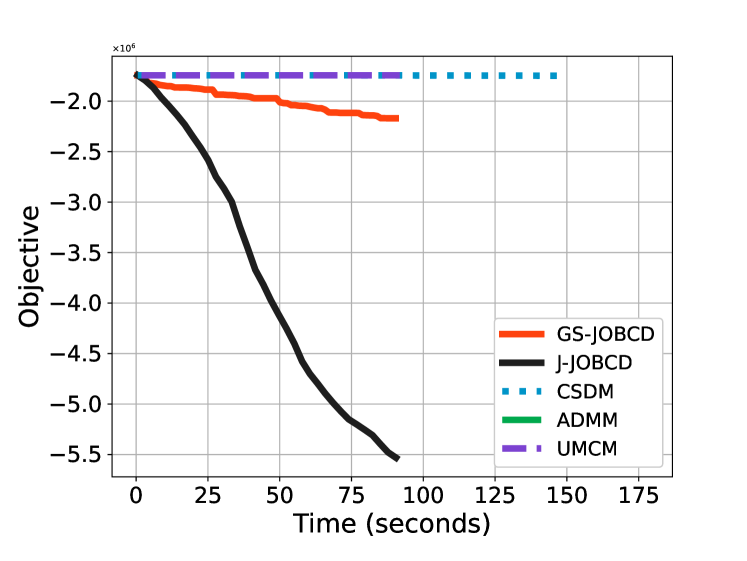
(c) gisette(3000-1000-900)

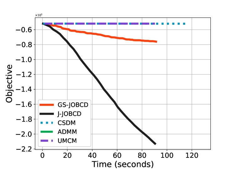
(d) mnist(1000-780-650)

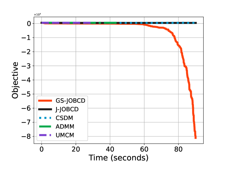
(e) randn(10-10-9)

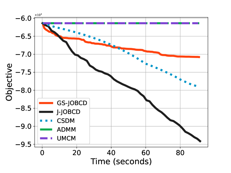
(f) randn(100-100-90)

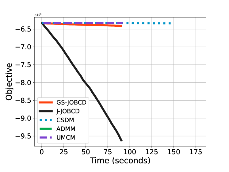
(g) randn(1000-1000-900)

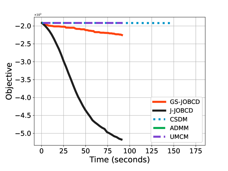
(h) sector(500-1000-900)

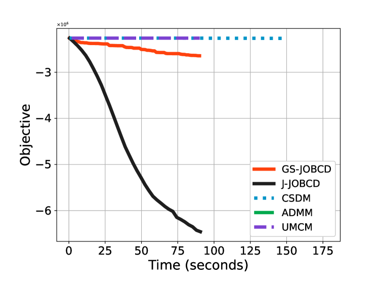
(i) TDT2(1000-1000-900)

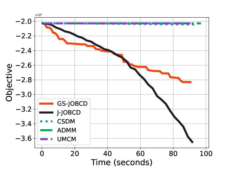
(j) w1a(2470-290-250)

Figure 5: The convergence curve of the compared methods for solving HEVP with varying $(m,n,p)$.

F.3.2 Hyperbolic Structural Probe Problem

Table 3: The convergence curve of the compared methods for solving HSPP. (+) indicates that after the convergence of the CSDM, utilizing the J-OBCD for optimization markedly enhances the objective value. The $1^{st},2^{\text{nd }}$, and $3^{\text{rd }}$ best results are colored with red, green and blue, respectively. $(n,p)$ represents the dimension and p-value of the J orthogonal matrix (square matrix). The value in $()$ stands for $\sum_{ij}^{n}|\mathbf{X}^{\top}\mathbf{J}\mathbf{X}-\mathbf{J}|_{ij}.$

datasetname	(m-n-p)	ADMM	UMCM	CSDM	J-JOBCD	VR-J-JOBCD	CSDM+J-JOBCD
time limit=30s
20News	(9423-50-25)	6.47e+04(2.4e-03)	6.47e+04(2.4e-03)	6.45e+04(2.0e-03)	6.40e+04(2.4e-03)	6.26e+04(2.4e-03)	6.31e+04(2.0e-03)(+)
Cifar	(10000-50-25)	1.49e+07(2.4e-03)	1.49e+07(2.4e-03)	1.49e+07(2.0e-03)	1.46e+07(2.4e-03)	1.45e+07(2.5e-03)	1.46e+07(2.0e-03)(+)
cnnCaltech	(3000-96-48)	3.08e+04(3.5e-09)	3.08e+04(3.5e-09)	3.03e+04(2.3e-05)	1.64e+04(4.0e-08)	1.64e+04(4.7e-08)	1.74e+04(2.3e-05)(+)
E2006	(5000-100-50)	5.54e+04(3.5e-09)	5.54e+04(3.5e-09)	5.54e+04(1.9e-05)	5.53e+04(9.0e-08)	5.53e+04(1.2e-07)	5.53e+04(1.9e-05)(+)
gisette	(6000-50-25)	1.61e+05(2.4e-03)	1.61e+05(2.4e-03)	1.52e+05(1.6e-03)	9.06e+04(2.4e-03)	7.48e+04(2.4e-03)	8.65e+04(1.6e-03)(+)
Mnist	(6000-92-46)	6.94e+06(3.6e-09)	6.94e+06(3.6e-09)	6.93e+06(2.1e-05)	6.50e+06(4.0e-05)	6.48e+06(8.7e-05)	6.93e+06(2.1e-05)
news20	(7967-50-25)	6.12e+04(2.4e-03)	6.12e+04(2.4e-03)	6.12e+04(2.0e-03)	6.12e+04(2.4e-03)	6.12e+04(2.4e-03)	6.12e+04(2.0e-03)
randn5000	(5000-100-50)	1.84e+06(3.5e-09)	1.84e+06(3.5e-09)	1.84e+06(2.0e-05)	1.77e+06(1.4e-07)	1.56e+06(9.9e-05)	1.84e+06(2.0e-05)
randn10000	(10000-50-25)	2.66e+06(2.4e-03)	2.66e+06(2.4e-03)	2.66e+06(2.5e-03)	2.64e+06(2.4e-03)	2.34e+06(2.5e-03)	2.66e+06(2.5e-03)
w1a	(2477-100-50)	2.71e+04(3.5e-09)	2.71e+04(3.5e-09)	2.47e+04(1.6e-05)	2.05e+04(3.6e-08)	1.92e+04(5.1e-08)	2.47e+04(1.6e-05)
20News	(9423-50-35)	7.89e+04(3.7e-09)	7.89e+04(3.7e-09)	7.85e+04(2.4e-05)	7.85e+04(8.6e-09)	7.71e+04(2.7e-08)	7.64e+04(2.4e-05)(+)
Cifar	(10000-50-35)	1.48e+07(5.5e-03)	1.48e+07(5.5e-03)	1.48e+07(6.2e-03)	1.43e+07(5.5e-03)	1.43e+07(5.7e-03)	1.43e+07(6.2e-03)(+)
cnnCaltech	(3000-96-70)	3.75e+04(2.0e-09)	3.75e+04(2.0e-09)	3.71e+04(1.3e-05)	2.40e+04(2.5e-08)	1.87e+04(3.4e-08)	2.15e+04(1.3e-05)(+)
E2006	(5000-100-75)	6.79e+04(1.0e-03)	6.79e+04(6.3e-04)	6.79e+04(5.8e-04)	6.65e+04(6.3e-04)	6.34e+04(6.3e-04)	6.69e+04(5.8e-04)(+)
gisette	(6000-50-35)	1.89e+05(5.5e-03)	1.89e+05(5.5e-03)	1.83e+05(4.7e-03)	1.24e+05(5.5e-03)	1.03e+05(5.5e-03)	1.17e+05(4.7e-03)(+)
Mnist	(6000-92-70)	6.75e+06(2.0e-09)	6.75e+06(2.0e-09)	6.74e+06(1.4e-05)	6.30e+06(7.7e-05)	6.20e+06(3.7e-04)	6.24e+06(7.0e-05)(+)
news20	(7967-50-35)	7.26e+04(5.5e-03)	7.26e+04(5.5e-03)	7.26e+04(4.9e-03)	7.26e+04(5.5e-03)	7.25e+04(5.5e-03)	7.26e+04(4.9e-03)
randn5000	(5000-100-75)	1.75e+06(6.3e-04)	1.75e+06(6.3e-04)	1.75e+06(6.1e-04)	1.44e+06(6.6e-04)	1.70e+06(6.3e-04)	1.75e+06(6.1e-04)
randn10000	(10000-50-36)	2.56e+06(3.7e-09)	2.56e+06(3.7e-09)	2.56e+06(2.0e-05)	2.56e+06(5.9e-09)	2.54e+06(2.2e-08)	2.56e+06(2.0e-05)(+)
w1a	(2477-100-75)	3.36e+04(6.3e-04)	3.36e+04(6.3e-04)	3.16e+04(5.5e-04)	2.53e+04(6.3e-04)	2.48e+04(6.3e-04)	2.90e+04(5.5e-04)(+)
20News	(9423-50-45)	8.79e+04(4.8e-03)	8.79e+04(4.8e-03)	8.73e+04(4.6e-03)	8.62e+04(4.8e-03)	8.60e+04(4.8e-03)	8.68e+04(4.6e-03)(+)
Cifar	(10000-50-45)	1.47e+07(4.8e-03)	1.47e+07(4.8e-03)	1.47e+07(4.6e-03)	1.46e+07(4.8e-03)	1.41e+07(7.2e-03)	1.46e+07(4.6e-03)(+)
cnnCaltech	(3000-96-85)	4.13e+04(9.2e-04)	4.14e+04(4.4e-04)	4.11e+04(6.5e-04)	2.59e+04(4.4e-04)	2.25e+04(4.4e-04)	2.65e+04(6.5e-04)(+)
E2006	(5000-100-90)	7.44e+04(1.2e-09)	7.44e+04(1.2e-09)	7.44e+04(7.5e-06)	6.95e+04(6.5e-08)	6.92e+04(3.8e-07)	6.93e+04(7.5e-06)(+)
gisette	(6000-50-45)	2.25e+05(4.8e-03)	2.25e+05(4.8e-03)	2.10e+05(5.2e-03)	1.42e+05(4.8e-03)	1.50e+05(4.8e-03)	1.54e+05(5.2e-03)(+)
Mnist	(6000-92-85)	6.73e+06(1.0e-03)	6.73e+06(1.0e-03)	6.73e+06(1.1e-03)	6.67e+06(1.0e-03)	6.22e+06(1.1e-03)	6.61e+06(1.1e-03)(+)
news20	(7967-50-45)	8.24e+04(4.8e-03)	8.24e+04(4.8e-03)	8.24e+04(4.5e-03)	8.24e+04(4.8e-03)	8.24e+04(4.8e-03)	8.24e+04(4.5e-03)
randn5000	(5000-100-85)	1.72e+06(1.3e-03)	1.72e+06(1.3e-03)	1.72e+06(1.4e-03)	1.70e+06(1.3e-03)	1.56e+06(1.3e-03)	1.72e+06(1.4e-03)
randn10000	(10000-50-45)	2.54e+06(3.3e-09)	2.54e+06(3.3e-09)	2.54e+06(1.9e-05)	2.53e+06(4.9e-09)	2.46e+06(3.3e-08)	2.54e+06(1.9e-05)
w1a	(2477-100-90)	4.10e+04(1.2e-09)	4.10e+04(1.2e-09)	3.76e+04(6.4e-06)	3.77e+04(4.2e-09)	3.27e+04(1.1e-08)	3.48e+04(6.4e-06)(+)
time limit=60s
20News	(9423-50-25)	6.47e+04(2.4e-03)	6.47e+04(2.4e-03)	6.42e+04(1.9e-03)	6.32e+04(2.4e-03)	6.35e+04(2.4e-03)	6.29e+04(1.9e-03)(+)
Cifar	(10000-50-25)	1.49e+07(2.4e-03)	1.49e+07(2.4e-03)	1.49e+07(1.7e-03)	1.45e+07(2.5e-03)	1.45e+07(2.5e-03)	1.45e+07(1.7e-03)(+)
cnnCaltech	(3000-96-48)	3.08e+04(3.5e-09)	3.08e+04(3.5e-09)	3.00e+04(2.4e-05)	1.92e+04(3.8e-08)	1.52e+04(4.8e-08)	1.67e+04(2.4e-05)(+)
E2006	(5000-100-50)	5.54e+04(3.5e-09)	5.54e+04(3.5e-09)	5.54e+04(2.3e-05)	5.51e+04(1.6e-07)	5.23e+04(3.9e-07)	5.51e+04(2.3e-05)(+)
gisette	(6000-50-25)	1.61e+05(2.4e-03)	1.61e+05(2.4e-03)	1.46e+05(2.1e-03)	9.76e+04(2.4e-03)	7.20e+04(2.4e-03)	8.40e+04(2.1e-03)(+)
Mnist	(6000-92-46)	6.94e+06(3.6e-09)	6.94e+06(3.6e-09)	6.93e+06(2.1e-05)	6.47e+06(1.4e-04)	6.45e+06(3.0e-04)	6.93e+06(2.1e-05)
news20	(7967-50-25)	6.12e+04(2.4e-03)	6.12e+04(2.4e-03)	6.12e+04(2.0e-03)	6.12e+04(2.4e-03)	6.12e+04(2.4e-03)	6.12e+04(2.0e-03)
randn5000	(5000-100-50)	1.84e+06(3.5e-09)	1.84e+06(3.5e-09)	1.84e+06(1.9e-05)	1.59e+06(8.3e-05)	1.51e+06(4.9e-04)	1.84e+06(1.9e-05)
randn10000	(10000-50-25)	2.66e+06(2.4e-03)	2.66e+06(2.4e-03)	2.66e+06(2.5e-03)	2.58e+06(2.4e-03)	2.37e+06(2.4e-03)	2.66e+06(2.5e-03)
w1a	(2477-100-50)	2.71e+04(3.5e-09)	2.71e+04(3.5e-09)	2.41e+04(1.5e-05)	2.33e+04(1.3e-08)	1.89e+04(6.0e-08)	2.41e+04(1.5e-05)
20News	(9423-50-35)	7.89e+04(3.7e-09)	7.89e+04(3.7e-09)	7.84e+04(2.1e-05)	7.63e+04(3.3e-08)	7.60e+04(5.3e-08)	7.84e+04(2.1e-05)
Cifar	(10000-50-35)	1.48e+07(5.5e-03)	1.48e+07(5.5e-03)	1.48e+07(6.5e-03)	1.43e+07(5.6e-03)	1.42e+07(5.7e-03)	1.43e+07(6.5e-03)(+)
cnnCaltech	(3000-96-70)	3.75e+04(2.0e-09)	3.75e+04(2.0e-09)	3.69e+04(1.1e-05)	1.93e+04(3.2e-08)	1.89e+04(3.6e-08)	2.19e+04(1.1e-05)(+)
E2006	(5000-100-75)	6.79e+04(1.0e-03)	6.79e+04(6.3e-04)	6.79e+04(5.6e-04)	6.48e+04(6.3e-04)	6.36e+04(6.3e-04)	6.39e+04(5.6e-04)(+)
gisette	(6000-50-35)	1.89e+05(5.5e-03)	1.89e+05(5.5e-03)	1.80e+05(4.4e-03)	1.14e+05(5.5e-03)	9.97e+04(5.5e-03)	1.24e+05(4.4e-03)(+)
Mnist	(6000-92-70)	6.75e+06(2.0e-09)	6.75e+06(2.0e-09)	6.74e+06(1.3e-05)	6.21e+06(5.4e-04)	6.17e+06(2.0e-04)	6.21e+06(3.4e-04)(+)
news20	(7967-50-35)	7.26e+04(5.5e-03)	7.26e+04(5.5e-03)	7.26e+04(4.8e-03)	7.25e+04(5.5e-03)	7.25e+04(5.5e-03)	7.25e+04(4.8e-03)(+)
randn5000	(5000-100-75)	1.75e+06(6.3e-04)	1.75e+06(6.3e-04)	1.75e+06(6.1e-04)	1.44e+06(7.2e-04)	1.35e+06(9.9e-04)	1.75e+06(6.1e-04)
randn10000	(10000-50-36)	2.56e+06(3.7e-09)	2.56e+06(3.7e-09)	2.56e+06(2.0e-05)	2.56e+06(5.4e-09)	2.41e+06(2.6e-07)	2.56e+06(2.0e-05)
w1a	(2477-100-75)	3.36e+04(6.3e-04)	3.36e+04(6.3e-04)	3.10e+04(5.4e-04)	3.32e+04(6.3e-04)	2.57e+04(6.3e-04)	3.10e+04(5.4e-04)
20News	(9423-50-45)	8.79e+04(4.8e-03)	8.79e+04(4.8e-03)	8.71e+04(4.5e-03)	8.73e+04(4.8e-03)	8.57e+04(4.8e-03)	8.66e+04(4.5e-03)(+)
Cifar	(10000-50-45)	1.47e+07(4.8e-03)	1.47e+07(4.8e-03)	1.47e+07(4.5e-03)	1.46e+07(4.8e-03)	1.46e+07(4.8e-03)	1.46e+07(4.5e-03)(+)
cnnCaltech	(3000-96-85)	4.13e+04(9.2e-04)	4.14e+04(4.4e-04)	4.09e+04(7.2e-04)	2.69e+04(4.4e-04)	2.44e+04(4.4e-04)	2.40e+04(7.2e-04)(+)
E2006	(5000-100-90)	7.44e+04(1.2e-09)	7.44e+04(1.2e-09)	7.44e+04(6.1e-06)	6.92e+04(8.2e-08)	6.90e+04(1.3e-07)	6.94e+04(6.1e-06)(+)
gisette	(6000-50-45)	2.25e+05(4.8e-03)	2.25e+05(4.8e-03)	2.10e+05(5.2e-03)	1.63e+05(4.8e-03)	1.37e+05(4.8e-03)	2.10e+05(5.2e-03)
Mnist	(6000-92-85)	6.73e+06(1.0e-03)	6.73e+06(1.0e-03)	6.73e+06(1.1e-03)	6.65e+06(1.0e-03)	6.12e+06(1.3e-03)	6.73e+06(1.1e-03)
news20	(7967-50-45)	8.24e+04(4.8e-03)	8.24e+04(4.8e-03)	8.24e+04(4.4e-03)	8.24e+04(4.8e-03)	8.24e+04(4.8e-03)	8.24e+04(4.4e-03)
randn5000	(5000-100-85)	1.72e+06(1.3e-03)	1.72e+06(1.3e-03)	1.72e+06(1.4e-03)	1.65e+06(1.3e-03)	1.56e+06(1.3e-03)	1.72e+06(1.4e-03)
randn10000	(10000-50-45)	2.54e+06(3.3e-09)	2.54e+06(3.3e-09)	2.54e+06(1.9e-05)	2.53e+06(9.0e-09)	2.34e+06(2.5e-07)	2.54e+06(1.9e-05)
w1a	(2477-100-90)	4.10e+04(1.2e-09)	4.10e+04(1.2e-09)	3.64e+04(6.0e-06)	3.45e+04(1.0e-08)	3.16e+04(1.0e-08)	3.34e+04(6.0e-06)(+)
time limit=90s
20News	(9423-50-25)	6.47e+04(2.4e-03)	6.47e+04(2.4e-03)	6.41e+04(1.8e-03)	6.31e+04(2.4e-03)	6.25e+04(2.4e-03)	6.41e+04(1.8e-03)
Cifar	(10000-50-25)	1.49e+07(2.4e-03)	1.49e+07(2.4e-03)	1.49e+07(2.0e-03)	1.45e+07(2.5e-03)	1.45e+07(2.6e-03)	1.45e+07(2.0e-03)(+)
cnnCaltech	(3000-96-48)	3.08e+04(3.5e-09)	3.08e+04(3.5e-09)	2.98e+04(2.2e-05)	1.89e+04(4.0e-08)	1.52e+04(4.5e-08)	1.74e+04(2.2e-05)(+)
E2006	(5000-100-50)	5.54e+04(3.5e-09)	5.54e+04(3.5e-09)	5.54e+04(2.1e-05)	5.34e+04(2.7e-07)	5.22e+04(3.0e-07)	5.30e+04(2.1e-05)(+)
gisette	(6000-50-25)	1.61e+05(2.4e-03)	1.61e+05(2.4e-03)	1.42e+05(2.3e-03)	9.50e+04(2.4e-03)	8.14e+04(2.4e-03)	7.44e+04(2.3e-03)(+)
Mnist	(6000-92-46)	6.94e+06(3.6e-09)	6.94e+06(3.6e-09)	6.93e+06(2.0e-05)	6.45e+06(3.6e-04)	6.42e+06(1.4e-03)	6.93e+06(2.0e-05)
news20	(7967-50-25)	6.12e+04(2.4e-03)	6.12e+04(2.4e-03)	6.12e+04(1.9e-03)	6.12e+04(2.4e-03)	6.12e+04(2.4e-03)	6.12e+04(1.9e-03)
randn5000	(5000-100-50)	1.84e+06(3.5e-09)	1.84e+06(3.5e-09)	1.84e+06(1.9e-05)	1.63e+06(1.4e-05)	1.52e+06(6.9e-04)	1.84e+06(1.9e-05)
randn10000	(10000-50-25)	2.66e+06(2.4e-03)	2.66e+06(2.4e-03)	2.66e+06(2.5e-03)	2.65e+06(2.4e-03)	2.25e+06(2.7e-03)	2.66e+06(2.5e-03)
w1a	(2477-100-50)	2.71e+04(3.5e-09)	2.71e+04(3.5e-09)	2.34e+04(1.5e-05)	2.24e+04(1.9e-08)	2.00e+04(4.3e-08)	1.90e+04(1.5e-05)(+)
20News	(9423-50-35)	7.89e+04(3.7e-09)	7.89e+04(3.7e-09)	7.84e+04(2.3e-05)	7.66e+04(4.5e-08)	7.57e+04(1.6e-07)	7.70e+04(2.3e-05)(+)
Cifar	(10000-50-35)	1.48e+07(5.5e-03)	1.48e+07(5.5e-03)	1.48e+07(7.0e-03)	1.43e+07(5.6e-03)	1.42e+07(6.2e-03)	1.43e+07(7.1e-03)(+)
cnnCaltech	(3000-96-70)	3.75e+04(2.0e-09)	3.75e+04(2.0e-09)	3.67e+04(1.4e-05)	2.33e+04(2.3e-08)	2.29e+04(2.5e-08)	2.16e+04(1.4e-05)(+)
E2006	(5000-100-75)	6.79e+04(1.0e-03)	6.79e+04(6.3e-04)	6.79e+04(5.5e-04)	6.37e+04(6.3e-04)	6.36e+04(6.3e-04)	6.38e+04(5.5e-04)(+)
gisette	(6000-50-35)	1.89e+05(5.5e-03)	1.89e+05(5.5e-03)	1.78e+05(4.2e-03)	1.16e+05(5.5e-03)	9.77e+04(5.5e-03)	1.10e+05(4.2e-03)(+)
Mnist	(6000-92-70)	6.75e+06(2.0e-09)	6.75e+06(2.0e-09)	6.74e+06(1.2e-05)	6.18e+06(7.5e-04)	6.15e+06(2.4e-03)	6.22e+06(6.7e-04)(+)
news20	(7967-50-35)	7.26e+04(5.5e-03)	7.26e+04(5.5e-03)	7.26e+04(4.6e-03)	7.25e+04(5.5e-03)	7.25e+04(5.5e-03)	7.25e+04(4.6e-03)(+)
randn5000	(5000-100-75)	1.75e+06(6.3e-04)	1.75e+06(6.3e-04)	1.75e+06(6.1e-04)	1.39e+06(1.2e-03)	1.38e+06(1.0e-03)	1.75e+06(6.1e-04)
randn10000	(10000-50-36)	2.56e+06(3.7e-09)	2.56e+06(3.7e-09)	2.56e+06(2.0e-05)	2.56e+06(4.4e-09)	2.51e+06(3.5e-08)	2.56e+06(2.0e-05)
w1a	(2477-100-75)	3.36e+04(6.3e-04)	3.36e+04(6.3e-04)	3.04e+04(5.2e-04)	2.64e+04(6.3e-04)	2.58e+04(6.3e-04)	2.56e+04(5.2e-04)(+)
20News	(9423-50-45)	8.79e+04(4.8e-03)	8.79e+04(4.8e-03)	8.70e+04(4.4e-03)	8.66e+04(4.8e-03)	8.58e+04(4.8e-03)	8.61e+04(4.4e-03)(+)
Cifar	(10000-50-45)	1.47e+07(4.8e-03)	1.47e+07(4.8e-03)	1.47e+07(4.4e-03)	1.46e+07(4.8e-03)	1.41e+07(8.6e-03)	1.41e+07(5.7e-03)(+)
cnnCaltech	(3000-96-85)	4.13e+04(9.2e-04)	4.14e+04(4.4e-04)	4.07e+04(8.2e-04)	2.47e+04(4.4e-04)	2.38e+04(4.4e-04)	2.91e+04(8.2e-04)(+)
E2006	(5000-100-90)	7.44e+04(1.2e-09)	7.44e+04(1.2e-09)	7.44e+04(8.7e-06)	6.89e+04(9.4e-08)	6.99e+04(7.9e-08)	7.09e+04(8.7e-06)(+)
gisette	(6000-50-45)	2.25e+05(4.8e-03)	2.25e+05(4.8e-03)	2.09e+05(5.2e-03)	1.83e+05(4.8e-03)	1.34e+05(4.8e-03)	2.09e+05(5.2e-03)
Mnist	(6000-92-85)	6.73e+06(1.0e-03)	6.73e+06(1.0e-03)	6.73e+06(1.1e-03)	6.72e+06(1.0e-03)	6.14e+06(1.1e-03)	6.73e+06(1.1e-03)
news20	(7967-50-45)	8.24e+04(4.8e-03)	8.24e+04(4.8e-03)	8.24e+04(4.2e-03)	8.24e+04(4.8e-03)	8.24e+04(4.8e-03)	8.24e+04(4.2e-03)
randn5000	(5000-100-85)	1.72e+06(1.3e-03)	1.72e+06(1.3e-03)	1.72e+06(1.4e-03)	1.46e+06(1.3e-03)	1.55e+06(1.3e-03)	1.72e+06(1.4e-03)
randn10000	(10000-50-45)	2.54e+06(3.3e-09)	2.54e+06(3.3e-09)	2.54e+06(1.9e-05)	2.53e+06(5.8e-09)	2.52e+06(9.7e-09)	2.54e+06(1.9e-05)
w1a	(2477-100-90)	4.10e+04(1.2e-09)	4.10e+04(1.2e-09)	3.56e+04(6.5e-06)	3.86e+04(2.3e-09)	2.95e+04(1.7e-08)	3.07e+04(6.5e-06)(+)

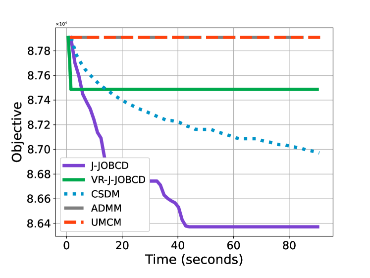
(a) 20News(9423-50-45)

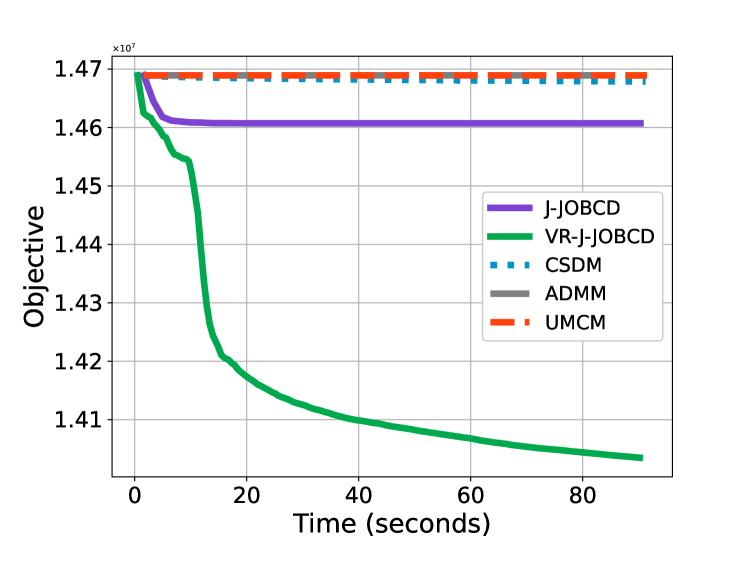
(b) Cifar(10000-50-45)

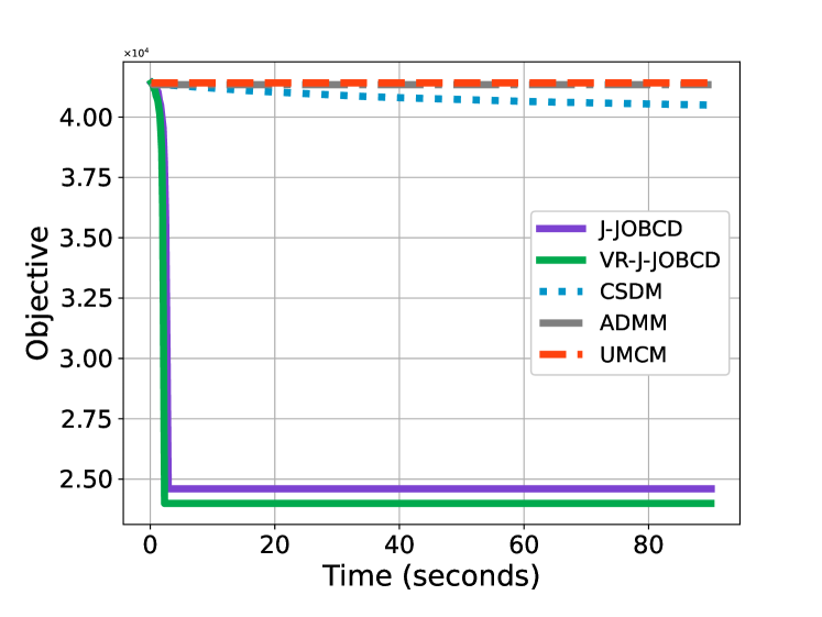
(c) CnnCaltech(3000-96-85)

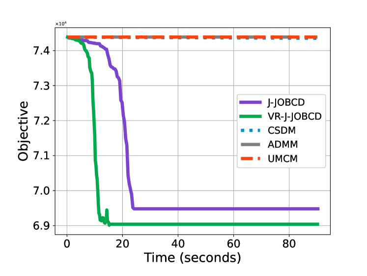
(d) E2006(5000-100-90)

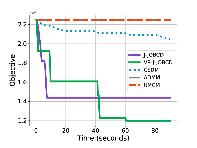
(e) Gisette(6000-50-45)

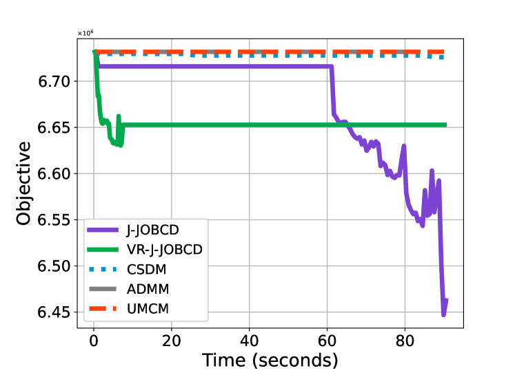
(f) Mnist(6000-92-85)

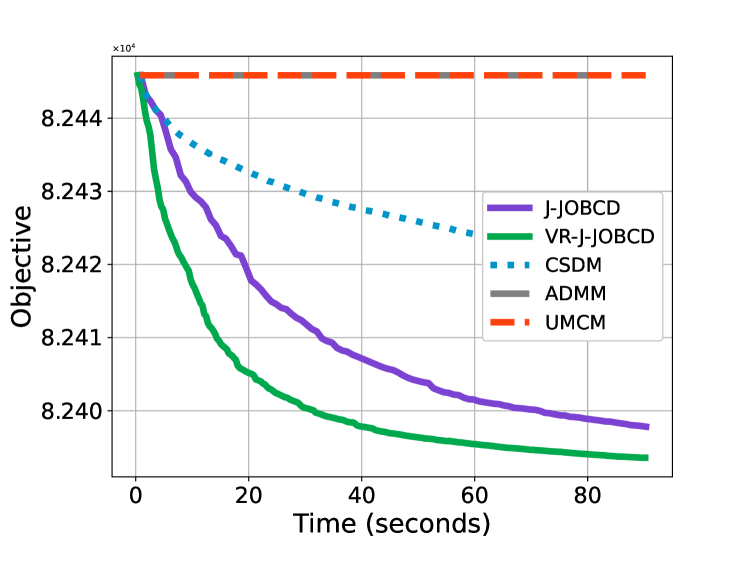
(g) News20(7967-50-45)

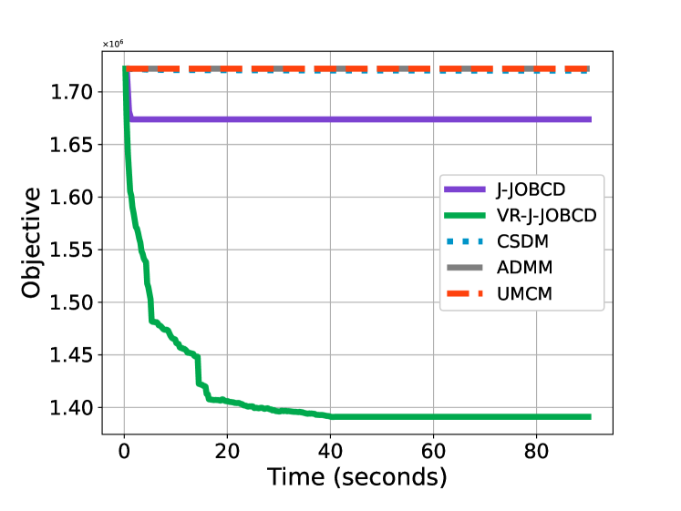
(h) randn(5000-100-85)

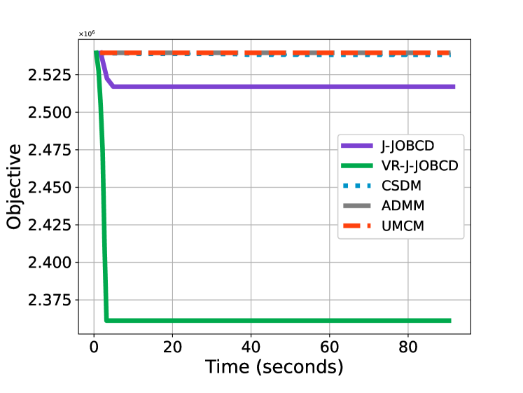
(i) randn(10000-50-45)

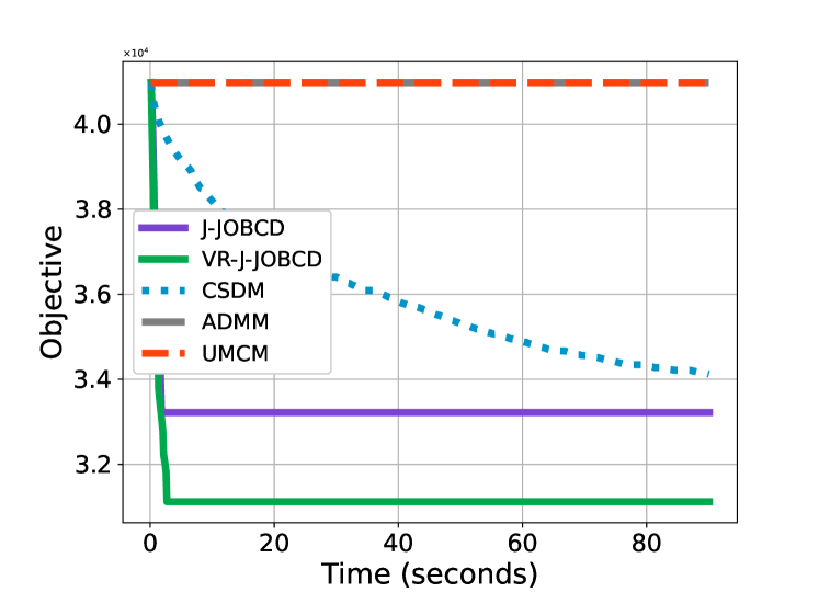
(j) W1a(2477-100-90)

Figure 7: The convergence curve of the compared methods for solving HSPP by time with varying $(m,n,p)$.

F.3.3 Ultra-hyperbolic Knowledge Graph Embedding

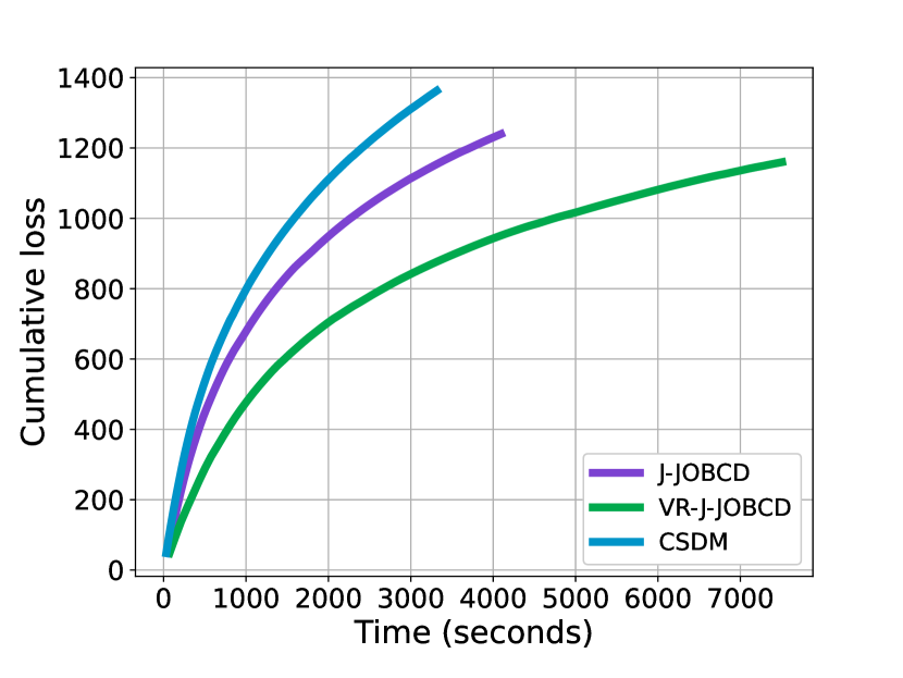
(a) Train accumulated loss

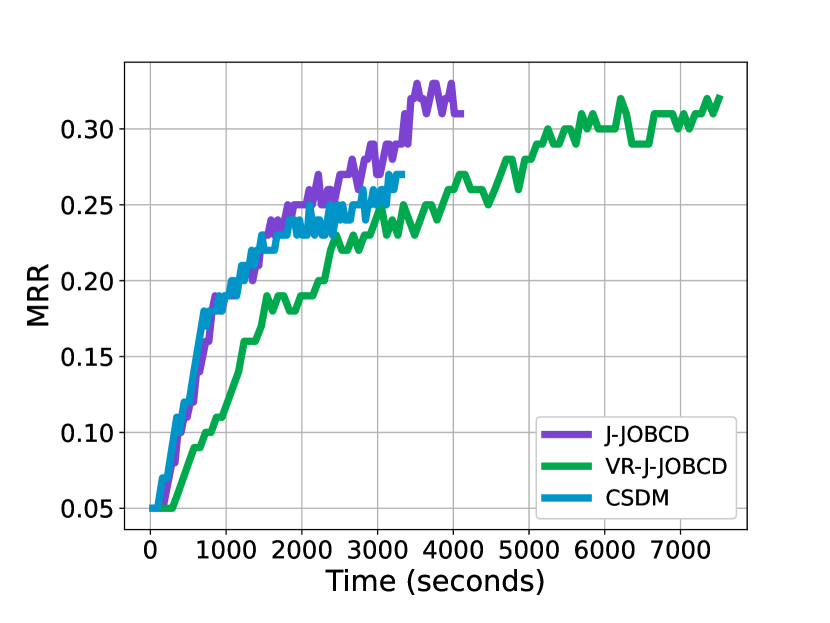
(b) Test MRR

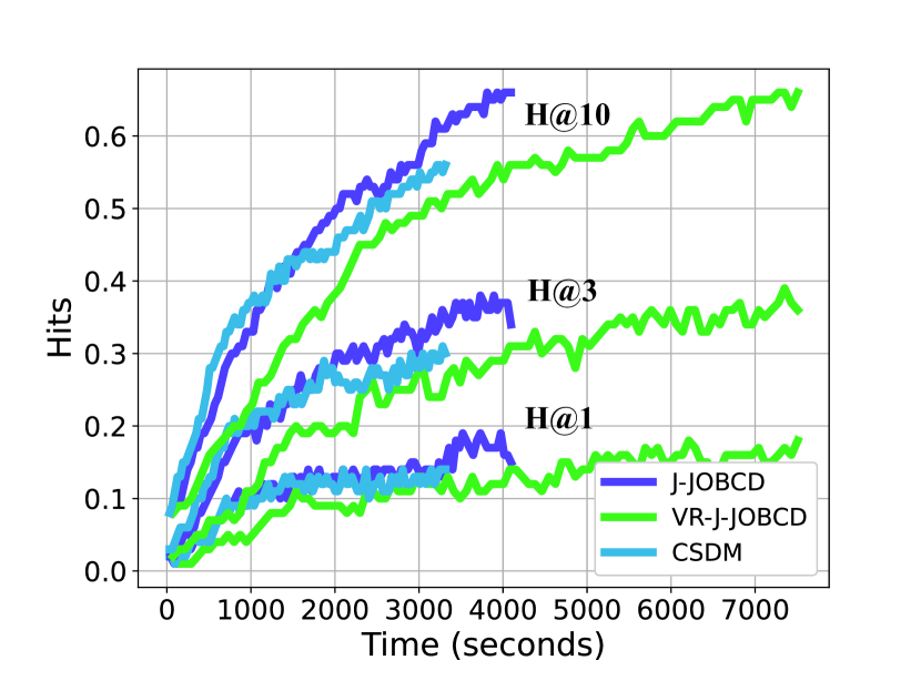
(c) Test Hits

Figure 9: Time performance of CS, J-JOBCD, and VR-J-JOBCD in training UltraE on FB15k.

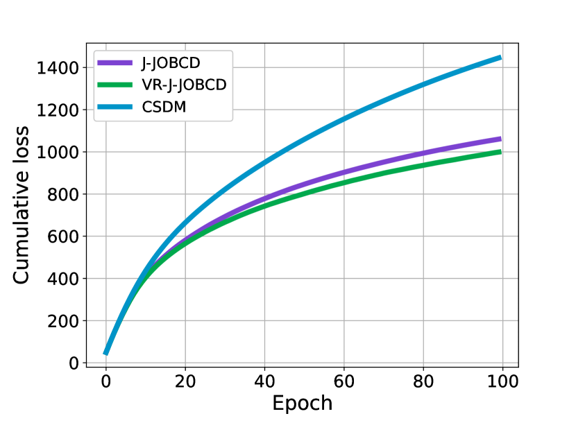
(a) Train accumulated loss

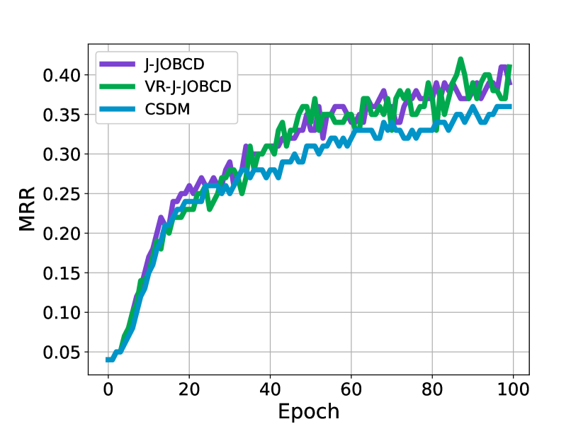
(b) Test MRR

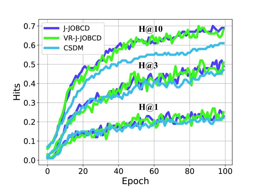
(c) Test Hits

Figure 10: Epoch performance of CSDM, J-JOBCD, and VR-J-JOBCD in training UltraE on WN18RR.

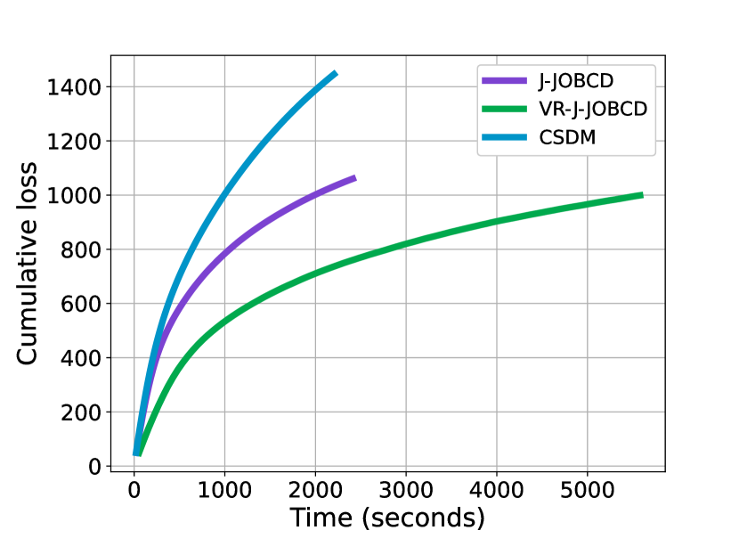
(a) Train accumulated loss

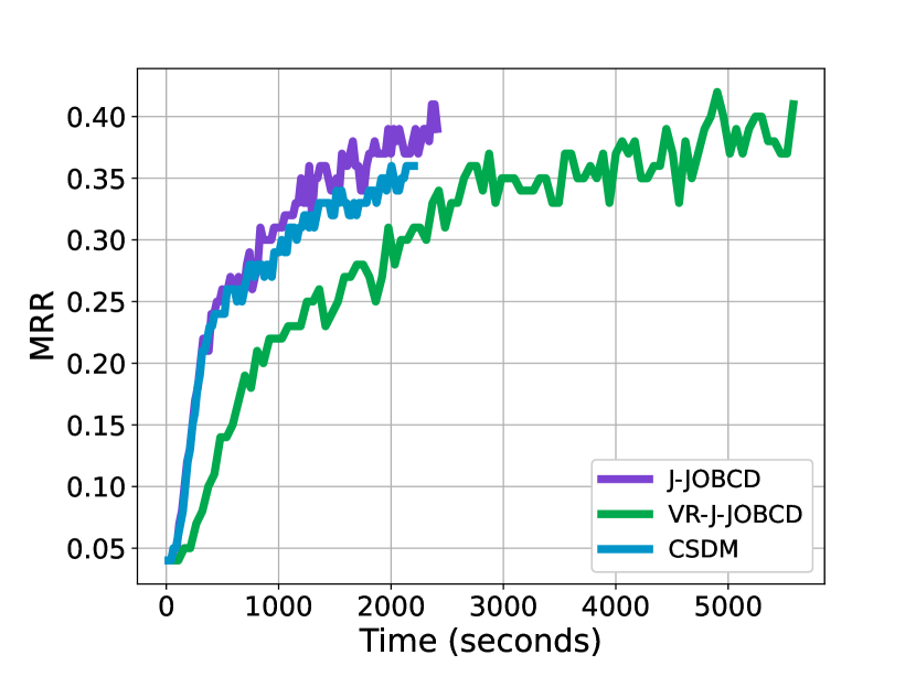
(b) Test MRR

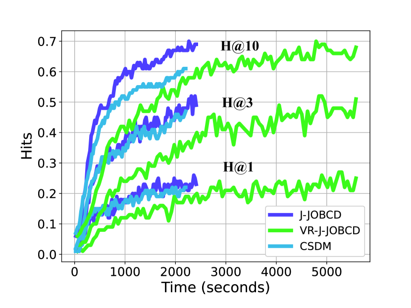
(c) Test Hits

Figure 11: Time performance of CSDM, J-JOBCD, and VR-J-JOBCD in training UltraE on WN18RR.

References

- (1) P-A Absil, Robert Mahony, and Rodolphe Sepulchre. Optimization algorithms on matrix manifolds. Princeton University Press, 2008.
- (2) Hédy Attouch, Jérôme Bolte, Patrick Redont, and Antoine Soubeyran. Proximal alternating minimization and projection methods for nonconvex problems: An approach based on the kurdyka-łojasiewicz inequality. Mathematics of operations research, 35(2):438–457, 2010.
- (3) Adam Bojanczyk, Nicholas J Higham, and Harikrishna Patel. Solving the indefinite least squares problem by hyperbolic qr factorization. SIAM Journal on Matrix Analysis and Applications, 24(4):914–931, 2003.
- (4) HanQin Cai, Yuchen Lou, Daniel McKenzie, and Wotao Yin. A zeroth-order block coordinate descent algorithm for huge-scale black-box optimization. In International Conference on Machine Learning, pages 1193–1203. PMLR, 2021.
- (5) Xufeng Cai, Chaobing Song, Stephen Wright, and Jelena Diakonikolas. Cyclic block coordinate descent with variance reduction for composite nonconvex optimization. In International Conference on Machine Learning, pages 3469–3494. PMLR, 2023.
- (6) Ines Chami, Albert Gu, Dat P Nguyen, and Christopher Re. Horopca: Hyperbolic dimensionality reduction via horospherical projections. In International Conference on Machine Learning (ICML), volume 139, pages 1419–1429, 2021.
- (7) Boli Chen, Yao Fu, Guangwei Xu, Pengjun Xie, Chuanqi Tan, Mosha Chen, and Liping Jing. Probing bert in hyperbolic spaces. ICLR, 2021.
- (8) Weize Chen, Xu Han, Yankai Lin, Hexu Zhao, Zhiyuan Liu, Peng Li, Maosong Sun, and Jie Zhou. Fully hyperbolic neural networks. arXiv preprint arXiv:2105.14686, 2021.
- (9) Ashok Cutkosky and Francesco Orabona. Momentum-based variance reduction in non-convex sgd. Advances in neural information processing systems, 32, 2019.
- (10) Aaron Defazio, Francis Bach, and Simon Lacoste-Julien. Saga: A fast incremental gradient method with support for non-strongly convex composite objectives. Advances in neural information processing systems, 27, 2014.
- (11) Cong Fang, Chris Junchi Li, Zhouchen Lin, and Tong Zhang. Spider: Near-optimal non-convex optimization via stochastic path-integrated differential estimator. Advances in neural information processing systems, 31, 2018.
- (12) Hamza Fawzi and Harry Goulbourne. Faster proximal algorithms for matrix optimization using jacobi-based eigenvalue methods. Advances in Neural Information Processing Systems, 34:11397–11408, 2021.
- (13) Bin Gao, Xin Liu, Xiaojun Chen, and Ya-xiang Yuan. A new first-order algorithmic framework for optimization problems with orthogonality constraints. SIAM Journal on Optimization, 28(1):302–332, 2018.
- (14) Bin Gao, Xin Liu, and Ya-xiang Yuan. Parallelizable algorithms for optimization problems with orthogonality constraints. SIAM Journal on Scientific Computing, 41(3):A1949–A1983, 2019.
- (15) Saeed Ghadimi, Guanghui Lan, and Hongchao Zhang. Mini-batch stochastic approximation methods for nonconvex stochastic composite optimization. Mathematical Programming, 155(1-2):267–305, 2016.
- (16) Gene H Golub and Charles F Van Loan. Matrix computations. JHU press, 2013.
- (17) Eldon R Hansen. On cyclic jacobi methods. Journal of the Society for Industrial and Applied Mathematics, 11(2):448–459, 1963.
- (18) Vjeran Hari and Erna Begović Kovač. On the convergence of complex jacobi methods. Linear and multilinear algebra, 69(3):489–514, 2021.
- (19) Bingsheng He and Xiaoming Yuan. On the convergence rate of the douglas-rachford alternating direction method. SIAM Journal on Numerical Analysis, 50(2):700–709, 2012.
- (20) John Hewitt and Christopher D. Manning. A structural probe for finding syntax in word representations. In Jill Burstein, Christy Doran, and Thamar Solorio, editors, Proceedings of the 2019 Conference of the North American Chapter of the Association for Computational Linguistics: Human Language Technologies (NAACL-HLT), pages 4129–4138, 2019.
- (21) Nicholas J Higham. J-orthogonal matrices: Properties and generation. SIAM review, 45(3):504–519, 2003.
- (22) Minhui Huang, Shiqian Ma, and Lifeng Lai. A riemannian block coordinate descent method for computing the projection robust wasserstein distance. In International Conference on Machine Learning, pages 4446–4455. PMLR, 2021.
- (23) Bo Hui and Wei-Shinn Ku. Low-rank nonnegative tensor decomposition in hyperbolic space. In Proceedings of the 28th ACM SIGKDD Conference on Knowledge Discovery and Data Mining, pages 646–654, 2022.
- (24) Sashank J Reddi, Suvrit Sra, Barnabas Poczos, and Alexander J Smola. Proximal stochastic methods for nonsmooth nonconvex finite-sum optimization. Advances in neural information processing systems, 29, 2016.
- (25) Rie Johnson and Tong Zhang. Accelerating stochastic gradient descent using predictive variance reduction. In C.J. Burges, L. Bottou, M. Welling, Z. Ghahramani, and K.Q. Weinberger, editors, Advances in Neural Information Processing Systems, volume 26. Curran Associates, Inc., 2013.
- (26) Diederik P. Kingma and Jimmy Ba. Adam: A method for stochastic optimization. In Yoshua Bengio and Yann LeCun, editors, International Conference on Learning Representations (ICLR), 2015.
- (27) Marc Law. Ultrahyperbolic neural networks. Advances in Neural Information Processing Systems, 34:22058–22069, 2021.
- (28) Marc Law and Jos Stam. Ultrahyperbolic representation learning. Advances in neural information processing systems, 33:1668–1678, 2020.
- (29) Qunwei Li, Yi Zhou, Yingbin Liang, and Pramod K Varshney. Convergence analysis of proximal gradient with momentum for nonconvex optimization. In International Conference on Machine Learning, pages 2111–2119. PMLR, 2017.
- (30) Zhize Li, Hongyan Bao, Xiangliang Zhang, and Peter Richtárik. Page: A simple and optimal probabilistic gradient estimator for nonconvex optimization. In International conference on machine learning, pages 6286–6295. PMLR, 2021.
- (31) Wei Liu, Yinyu Zhang, Hongqiao Yang, and Shuzhong Zhang. A class of smooth exact penalty function methods for optimization problems with orthogonality constraints. Optimization, 69(3):399–426, 2020.
- (32) Wan-Duo Kurt Ma, JP Lewis, and W Bastiaan Kleijn. The hsic bottleneck: Deep learning without back-propagation. In Proceedings of the AAAI conference on artificial intelligence, volume 34, pages 5085–5092, 2020.
- (33) Julien Mairal. Optimization with first-order surrogate functions. In International Conference on Machine Learning (ICML), volume 28, pages 783–791, 2013.
- (34) Lam M Nguyen, Jie Liu, Katya Scheinberg, and Martin Takáč. Sarah: A novel method for machine learning problems using stochastic recursive gradient. In International conference on machine learning, pages 2613–2621. PMLR, 2017.
- (35) Maximillian Nickel and Douwe Kiela. Learning continuous hierarchies in the lorentz model of hyperbolic geometry. In International Conference on Machine Learning, pages 3779–3788. PMLR, 2018.
- (36) Vedran Novaković and Sanja Singer. A kogbetliantz-type algorithm for the hyperbolic svd. Numerical algorithms, 90(2):523–561, 2022.
- (37) Julie Nutini, Issam Laradji, and Mark Schmidt. Let’s make block coordinate descent converge faster: faster greedy rules, message-passing, active-set complexity, and superlinear convergence. Journal of Machine Learning Research, 23(131):1–74, 2022.
- (38) Meisam Razaviyayn, Mingyi Hong, and Zhi-Quan Luo. A unified convergence analysis of block successive minimization methods for nonsmooth optimization. SIAM Journal on Optimization, 23(2):1126–1153, 2013.
- (39) Mark Schmidt, Nicolas Le Roux, and Francis Bach. Minimizing finite sums with the stochastic average gradient. Mathematical Programming, 162:83–112, 2017.
- (40) Ivan Slapnicar and Ninoslav Truhar. Relative perturbation theory for hyperbolic eigenvalue problem. Linear Algebra and its Applications, 309(1):57–72, 2000.
- (41) Michael Stewart and Paul Van Dooren. On the factorization of hyperbolic and unitary transformations into rotations. SIAM Journal on Matrix Analysis and Applications, 27(3):876–890, 2005.
- (42) Puoya Tabaghi and Ivan Dokmanić. Hyperbolic distance matrices. In Proceedings of the 26th ACM SIGKDD International Conference on Knowledge Discovery & Data Mining, pages 1728–1738, 2020.
- (43) Puoya Tabaghi, Michael Khanzadeh, Yusu Wang, and Sivash Mirarab. Principal component analysis in space forms. ArXiv, abs/2301.02750, 2023.
- (44) Zhe Wang, Kaiyi Ji, Yi Zhou, Yingbin Liang, and Vahid Tarokh. Spiderboost and momentum: Faster variance reduction algorithms. Advances in Neural Information Processing Systems, 32, 2019.
- (45) Zaiwen Wen and Wotao Yin. A feasible method for optimization with orthogonality constraints. Mathematical Programming, 142:397 – 434, 2012.
- (46) WikiContributors. Quartic equation. https://en.wikipedia.org/wiki/Quartic_equation.
- (47) Ruiyuan Wu, Anna Scaglione, Hoi-To Wai, Nurullah Karakoc, Kari Hreinsson, and Wing-Kin Ma. Federated block coordinate descent scheme for learning global and personalized models. In Proceedings of the AAAI Conference on Artificial Intelligence, volume 35, pages 10355–10362, 2021.
- (48) Bo Xiong, Shichao Zhu, Mojtaba Nayyeri, Chengjin Xu, Shirui Pan, Chuan Zhou, and Steffen Staab. Ultrahyperbolic knowledge graph embeddings. In Proceedings of the 28th ACM SIGKDD Conference on Knowledge Discovery and Data Mining, pages 2130–2139, 2022.
- (49) Bo Xiong, Shichao Zhu, Nico Potyka, Shirui Pan, Chuan Zhou, and Steffen Staab. Semi-riemannian graph convolutional networks. ArXiv, abs/2106.03134, 2021.
- (50) Tao Yu and Christopher M De Sa. Numerically accurate hyperbolic embeddings using tiling-based models. Advances in Neural Information Processing Systems, 32, 2019.
- (51) Ganzhao Yuan. A block coordinate descent method for nonsmooth composite optimization under orthogonality constraints. ArXiv, abs/2304.03641, 2023.
- (52) Ganzhao Yuan. Coordinate descent methods for fractional minimization. In International Conference on Machine Learning, pages 40488–40518, 2023.
- (53) Jinshan Zeng, Tim Tsz-Kit Lau, Shaobo Lin, and Yuan Yao. Global convergence of block coordinate descent in deep learning. In International conference on machine learning, pages 7313–7323. PMLR, 2019.
- (54) Yiding Zhang, Xiao Wang, Chuan Shi, Nian Liu, and Guojie Song. Lorentzian graph convolutional networks. In Proceedings of the Web Conference 2021, pages 1249–1261, 2021.
- (55) Dongruo Zhou, Pan Xu, and Quanquan Gu. Stochastic nested variance reduction for nonconvex optimization. The Journal of Machine Learning Research, 21(1):4130–4192, 2020.