LAVIB: A Large-scale Video Interpolation Benchmark

Abstract

This paper introduces a LArge-scale Video Interpolation Benchmark (LAVIB) for the low-level video task of video frame interpolation (VFI). LAVIB comprises a large collection of high-resolution videos sourced from the web through an automated pipeline with minimal requirements for human verification. Metrics are computed for each video’s motion magnitudes, luminance conditions, frame sharpness, and contrast. The collection of videos and the creation of quantitative challenges based on these metrics are under-explored by current low-level video task datasets. In total, LAVIB includes 283K clips from 17K ultra-HD videos, covering 77.6 hours. Benchmark train, val, and test sets maintain similar video metric distributions. Further splits are also created for out-of-distribution (OOD) challenges, with train and test splits including videos of dissimilar attributes.

1 Introduction

Long uncompressed video streams capture events over varying motion intensities, light conditions, and color dynamic ranges. Although loading and storing individual videos is rudimentary, processing and reading large volumes of videos can bottleneck their availability. The high-volume transfer of videos with large filesizes can also result in bandwidth overheads and long decoding times. Low-level vision tasks such as Video Frame Interpolation (VFI) [2, 9, 15, 18, 20, 28, 38, 39, 41, 46, 67], Video Super-Resolution (VSR) [4, 12, 16, 17, 21, 26, 29, 50, 58, 60], and Video Denoising (VD) [13, 30, 31, 49, 54, 57, 59] aim to address such challenges by enabling the storage and stream of lower-resolution, lower-frame-rate, compressed videos. Despite the wide application of such approaches to adjacent tasks such as localization and mapping [24, 63], object tracking [66], novel view synthesis [40, 48], and slow-motion video generation [18, 19], existing datasets for low-level video tasks [1, 37, 38, 43, 51, 52, 55, 56, 57, 64] contain videos of low total durations, with a small number of frames per video. With the exception of [64] most of these datasets only include either a few hundreds [1, 38, 43, 57] or thousands [37, 51, 52, 55, 56] of videos with limited variations in the motions, luminance, and object-level sharpness. To address this gap, this paper introduces a LArge Video Interpolation Benchmark (LAVIB), for learning to extend high-resolution videos across varying motion, blur, luminance, and contrast settings. LAVIB is built on per-frame metrics that quantitatively measure motion magnitudes, frame sharpness, video contrast, and overall luminance. In Fig. 1, LAVIB videos are visualized over axes corresponding to the metrics used.

The selected metrics establish a diverse, general, and robust benchmark for VFI as most prior efforts have focused on specific settings. Seminal works [35, 51] sourced videos from high frame-rate sensors that are less relevant to videos recorded by commonly used devices. Other works use videos of standardized resolutions and frame rates. These are either datasets of larger sizes with low-resolution videos [55, 64] or smaller datasets of high-resolution [38, 51, 52, 56, 57]. Comparisons to other video datasets across metrics are discussed in §2.

LAVIB contains 283,484 video segments totaling approximately 77.6 hours. The segments are sourced from 17,204 clips with $3840\times 2160$ (4K) resolution and 60 frames-per-second (fps). Statistics are discussed in §3. Similar to previous efforts comprised of 4K videos [35, 51, 56], LAVIB is compiled by temporally and spatially cropping tubelets from the 4K videos to fit clips into memory.

The data collection pipeline for LAVIB is detailed in §4. This includes the creation of a vocabulary of search query terms. Clips are sourced from YouTube videos queried by search terms. Preset clip sampling intervals are used to standardize durations. Segments are selected from high average flow magnitude temporal locations calculated with [14]. Spatial locations are selected by tubelets of high/low metrics values. The final train/val/test sets are constructed by balancing all metrics.

Widely-used VFI methods [15, 22, 67] are benchmarked on the LAVIB val and test sets in §5. Performance is reported across well-adopted evaluation metrics [3, 7, 8, 11, 27, 68]. LAVIB’s large size and video diversity enables pretraining models of greater generalizability that are in turn evaluated on test sets of smaller down-stream datasets targeting either scene diversity [64], high frame rates [51], or high video resolution [35, 38]. In addition to the main benchmark splits, four challenges with two settings each, are introduced for out-of-distribution (OOD) VFI. Train, val, and test sets with unbalanced metric distributions are created for each challenge and setting. Videos are assigned to sets based on their average motion magnitude, sharpness, contrast, and luminance metrics. These challenges evaluate model generalizability over diverse domains that are different in the train and test sets.

\begin{overpic}[width=433.62pt]{figures/teaser_examples_compressed.pdf} \put(92.0,0.0){\includegraphics[scale={0.115}]{figures/axis.pdf}} \end{overpic}

Figure 1: LAVIB videos distributed across metrics. Four metrics are computed per video. Average Flow Magnitude (AFM) quantifies motion 

. The Average Laplacian Variance (ALV) is used to describe the sharpness of frames 

. The Average Root Mean Square (ARMS) is used for contrast 

. The Average Relevant Luminance (ARL) relates to the video brightness 

. The four aforementioned metrics are used for out-of-distribution (ODD) challenges: Fast 

 $\rightarrow$ slow 

and slow 

 $\rightarrow$ fast 

motions. Low 

 $\rightarrow$ high 

and high 

 $\rightarrow$ low 

sharpness. Low 

 $\rightarrow$ high 

and high 

 $\rightarrow$ low 

contrast. Bright 

 $\rightarrow$ dark 

and dark 

 $\rightarrow$ bright 

luminance.

2 Related works

Initial VFI benchmarks [1] provided real image sequences and ground truth optical flow annotations with average resolutions of $640\times 480$. The dataset comprised a small number of videos used primarily for evaluation. Vid4 [32] is a standardized testing benchmark for VFI and VSR consisting of four videos of $740\times 480$ and $720\times 576$ resolutions. Similarly, [65] is also used for VSR with videos sampled from [62]. Later efforts [36] have also introduced benchmarks for VD in tandem with VSR and VFI. More recent works [37] included 3.2K HD videos captured with a GOPRO4 Hero Black with frame averaging to simulate lower shutter speeds. [47] also proposed a synthetic dataset with 3D objects from [5] and backgrounds from [23, 25]. The trajectories of objects were uniformly sampled from fixed bounds. Works have also studied VFI for specific domains such as animations [52]. [6] introduced benchmarks under large motion conditions with 20 240-fps videos sourced from YouTube. Recently, [51] introduced a high-resolution high-frame rate benchmark for video interpolation and super-resolution. It includes a total of 4,423 videos recorded with a Phantom Flex4K.

Most similar to LAVIB, adjacent efforts that compile 4K video datasets [35, 38, 51, 56] source videos from media in which professional equipment are used; e.g. movies [35, 38] or high-resolution video recordings [51]. Videos from these datasets are primarily recorded with sensors under optimal shutter speeds and calibrated luminance for capturing specific motion types. In contrast, LAVIB includes videos from various sensors such as hand-held, action, professional, or drone cameras, and screen captures. The videos differ in their dynamic range, levels of post-processing, and compression. LAVIB is intended as a general-purpose dataset and benchmark without being specific to sensor types or settings. Examples of videos are shown in Fig. 1.

LAVIB is compared in Table 1 to adjacent video datasets over different statistics. Dataset statistics include the number of videos and total running times. Video statistics relate to video information such as the resolution and frame rate. Average video metrics provide metrics on the variance of motions, lighting conditions, and frame sharpness. Definitions of the metrics are detailed in §3. LAVIB has threefold more videos than [64] and equally larger total video running time than [55]. The difference in LAVIB video conditions and recording sensors is reflected by the high variance across metrics in Table 1. With the exception of [51], tailored for videos of fast motions with high optical flow magnitude, LAVIB has the highest variance per metric across datasets.

Table 1: Dataset comparisons. LAVIB provides a large-scale general-purpose dataset of standardized 4K videos over 60 fps. It features a significant variance across Average Flow Magnitude (AFM), Average Relevant Luminance (ARL) in scenes, and Average Laplacian Variances (ALV) for sharpness.

Dataset	Dataset statistics			Video statistics		Video metrics
	Year	Tot. Mins	Tot. Vids	Src Res.	FPS	AFM	ARL	ALV
UCF101 [55]	2012	1,600	13,320	240p	25	2.43 $\pm$ 1.85	53.37 $\pm$ 13.42	53.99 $\pm$ 18.37
Xiph [35, 38]	2020	4	19	2160p	60	26.21 $\pm$ 25.19	60.64 $\pm$ 10.77	95.24 $\pm$ 62.32
Inter4K [56]	2021	83	1,000	2160p	60	56.38 $\pm$ 14.34	56.79 $\pm$ 14.48	25.05 $\pm$ 24.05
X4K1KFPS [51]	2021	191	4,423	2160p	960	266.87 $\pm$ 178.72	53.95 $\pm$ 12.07	135.67 $\pm$ 78.19
Vimeo90K [64]	2017	356	91,701	720p	30	49.63 $\pm$ 18.32	59.68 $\pm$ 20.89	26.26 $\pm$ 29.25
LAVIB (ours)	2024	4,660	283,484	2160p	60	63.10 $\pm$ 58.41	38.34 $\pm$ 28.69	199.78 $\pm$ 197.79

Table 2: LAVIB split statistics. Details per metric for each split.

Statistic		Train	Val	Train+Val	Test
	# Low Flow Mag	19,605 (10.3%)	3,846 (9.3%)	23,451 (10.1%)	4,898 (9.1%)
	# High Flow Mag	18,976 (10.1%)	3,891 (9.4%)	22,867 (9.9%)	5,482 (10.2%)
	# Low Lap. Var.	18,313 (9.6%)	3,541 (8.6%)	21,854 (9.5%)	6,494 (12.1%)
	# High Lap. Var.	17,348 (9.2%)	3,871 (9.4%)	21,219 (9.2%)	7,130 (13.3%)
	# Low Perc. Lum.	17,669 (9.3%)	3,638 (8.8%)	21,307 (9.2%)	7,041 (13.1%)
	# High Perc. Lum.	19,297 (10.2%)	4,400 (10.7%)	23,697 (10.3 %)	4,652 (8.6%)
	# Low RMS Cont.	18,794 (10.0%)	3,657 (8.8%)	22,451 (9.8%)	5,897 (11.0%)
	# High RMS Cont.	18,363 (9.7%)	4,036 (9.8 %)	22,399 (9.7%)	5,950 (11.1%)
Total		188,644	41,345	229,989	53,494

3 LAVIB statistics

Four statistics are used to obtain segments, create splits, and define challenges. An overview is shown in Table 2 with the number of videos with the highest/lowest metrics reported.

Frame-pair motion. A significant challenge for VFI methods is learning to model cross-frame motion consistency in videos. Thus, the proposed dataset includes videos of diverse magnitudes; both high camera or object motion, and more static scenes. Motion magnitudes can be quantified with dense optical flow. FlowFormer [14] is used on each frame pair resulting in 598 frame pairs per video. The spatial resolution of videos is reduced by $\times 0.25$ to fit frames in memory. The Averaged Flow Magnitude (AFM) is defined by spatio-temporally averaging optical flow. AFM variances are reported for all datasets in Table 1.

Frame sharpness. Sourced videos vary by the sensors, lens, codex, and camera profiles used. They can capture different motions, light conditions, and camera focus. All these factors amount to significant variations in the sharpness of videos. Thus, object edges or sensory noise may be highlighted or suppressed. The Laplacian of Gaussians (LoG) is a standardized kernel-based approach for highlighting regions of rapid change in pixel intensities. Given a video $\mathbf{V}$ of dimensions $\mathbb{R}^{D=T\times H\times W}$, with $T$ frames, $H$ height, and $W$ width, it convolves a kernel with size $K$ over each frame. ALV is formulated by applying LoG and averaging:

$$\begin{aligned} \text{ALV}(\mathbf{V},\sigma,K)&=\frac{1}{D}\sum_{r\in\mathbb{R}^{D}}\sum_{i=1}^{K}\sum_{j=1}^{K}\underbrace{-1\frac{1}{\pi\sigma^{4}}(1-\frac{i^{2}+j^{2}}{2\sigma^{2}})e^{-\frac{i^{2}+j^{2}}{2\sigma^{2}}}}_{\text{LoG}(i,j)}\;\underset{r-[i,j]}{\mathbf{V}}\end{aligned}$$ (1)

As the size of the kernel also factors the estimate, an ensemble of kernel sizes $\mathcal{N}=\{3,5,7\}$ is used to calculate the final value $\frac{1}{|\mathcal{N}|}\underset{K\in\mathcal{N}}{\sum}\text{ALV}(\mathbf{V},\sigma,K)$ with $\sigma=1.4$. Overall, in LAVIB 18,313 train, 3,541 val, and 6,494 test videos are at the upper 10% of the ALV ensemble.

Video contrast. Another characteristic of videos is the contrast between objects and backgrounds in scenes. The human visual system is more sensitive to the contrast between foreground and background [34, 45], compared to other adjacent measures such as the perceived luminance (brightness), or frame sharpness (blurriness). Computationally, contrast relates to the difference between neighboring raw pixel values. The metric is formulated as the Average Root Mean Square (ARMS) [42] difference between each pixel from each frame of $\mathbf{V}$ and the corresponding pixel in the channel-averaged $\overline{\mathbf{V}}$.

$$\text{ARMS}(\mathbf{V})=\frac{1}{T}\sum_{t\in\mathbb{R}^{T}}\sqrt{\frac{1}{HW}\sum_{s\in\mathbb{R}^{HW}}(\underset{t,s}{\mathbf{V}}-\underset{t,s}{\overline{\mathbf{V}}})}$$ (2)

LAVIB includes 22,399 videos of high contrast for train and val and, 22,451 videos of low contrast.

Luminance conditions. In addition to the overall video conditions, the perception of light can be affected by the sensor’s sensitivity or the camera’s processing. In human vision, the perception of luminance is done over three bands of color. To account for the uneven perception of each band, a common standard for quantitatively defining luminosity is the relevant luminance [44]. In videos, the Average Relative Luminance (ARL) can be computed as the weighted sum for each color channel from video frames based on [44], which in turn is averaged over time. The bottom 10th ARL percentile in LAVIB includes 17,669 train, 3,638 val, and 7,041 test videos. Similarly, there are 19,297 train, 4,400 val, and 4,652 test high-luminance videos.

As shown in Table 2, videos selected for all splits are balanced across metrics. This is done explicitly for the main benchmark and not the OOD challenges.

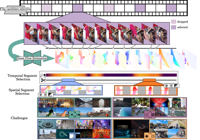
Figure 2: LAVIB segment selection and challenges pipeline. Candidate 10-second clips are sampled from a long video based on their embedding similarity. Dense optical flow is computed with [14] and spatially averaged for the AFM metric. The 1-second clips with the top-20% AFM are selected for the next step. Clips are further partitioned into four tubelets used in the final dataset based on their ARL, ALV, and ARMS. The metrics are also used for video selection in out-of-distribution (OOD) challenges for a. motion, b. sharpness, c. contrast, d. luminance.

4 LAVIB pipeline

The video selection pipeline includes several stages for the collection, extraction, and set assignment. Initially, videos are searched on YouTube by textual prompts designed to return relevant videos with 4K resolutions and 60 frames per second as overviewed in §4.1. Sourced videos are cropped to 10-second clips standardizing their durations and improving processing speeds in further steps of the collection pipeline. Segments with high motion magnitudes are selected from the clips and are spatially cropped based on the AVL, ARL, and ARMS statistics detailed in §4.2. Dataset splits are balanced between the four statistics, with OOD splits created by assigning videos with the highest average metric at the test or train set. The dataset pipeline is flexible and can be scaled over large numbers of videos, requiring manual input only at a few points.

4.1 Web-Crawling and video selection

The first stage of the data collection pipeline constructs queries to search and identify videos on YouTube with 4K resolution and 60 fps. The vocabulary of search terms is created from a finite combination of different categories e.g.; locations, activities, weather conditions, and camera types. This aims to diversify results over the defined categories (See appendix A1-0 for the full vocabulary). The vocabulary terms are compiled with three guidelines.

Videos should be in the wild. Retrieved videos should vary by lighting conditions, motions, and scenes. They should also be recorded with different sensors. Sensor types depend strongly on video themes; e.g. action cameras are more common for capturing fast-paced scenes in contrast to DSLR cameras. Conditions are added in the format; ‘rainy walk in New York’ or ‘night drive’. Some text prompts are also designed to include specific equipment such as ‘GoPro Hero10’ or ‘iPhone 13 Pro’.

Video content should correspond to raw footage. The dictionary of general search terms aims to improve control over the video context by retrieving specific video types. Videos with substantial post-production cuts, or transitions, can be less relevant or usable for VFI. The video types that are collected focus primarily on raw footage.

Exclusivity of video categories. Vocabulary queries should also include diversity in the themes present. This is done by constructing verb hierarchies. A balanced number of queries is constructed for objects/locations that are the focus of the videos.

Each vocabulary search term is combined with ‘4K’ and used as a query on YouTube. The query-related URLs are scraped from the contents in the response’s script. Candidate videos are downloaded only if a 4K format with 60 fps is available. This step is needed as YouTube’s search prioritizes video elements such as titles, tags, and descriptions over metadata.

Limitations. Queries are created from a finite set of search terms. The diversity of locations and activities is manually defined thus, limitations are expected. As noted above, the selected videos are more diverse than current VFI benchmarks however, an increased vocabulary can improve this further.

4.2 Segment selection and assignment

In total, 667 hours of footage are collected over the project’s 31-month duration. This initial list contained videos of hour-long to minute-long durations. To standardize their durations, 10-second clips are sampled manually over different interval steps. Clips are extracted consecutively for videos less than 5 minutes. For the rest of the videos; 10-second sampling intervals are used for videos with durations between 5-30 minutes, 2-minute intervals for videos between 30 minutes to an hour, and 10-minute intervals for videos longer than an hour. This selection resulted in a total of 34,408 clips. Clips from the same video are bound to include similarities. To account for this and inspired by [68], similarities between clips from the same video are measured metrically by their embedding space distance with highly similar clips being dropped. MViTv2-B [10] is used as the clip encoder from which a similarity matrix between final layer embeddings is created by computing the L2 distance over clip pairs. Clips with an average (row-wise) L2 distance below the entire matrix’s average are dropped. This step resulted in the selection of 17,204 clips.

The final two stages include both temporal and spatial cropping. They are overviewed in Fig. 2.

Temporal Segment Selection. Segments are compared and in turn selected by their average motion magnitudes. Primarily static segments are dropped as they are less relevant to VFI tasks with minimal pixel and object tracking requirements. FlowFormer [14] calculates flow maps over pairs of frames with magnitudes averaged spatially. Each 10-second sequence is temporally augmented to obtain all available 1-second clips. Clips with the highest 20% magnitudes are selected. This strategy was chosen as it worked well in a small-scale setting when manually examining a set of 1,000 clips.

Spatial Segment Selection. The selected high-resolution clips cannot directly fit into the memory of most current GPUs. Thus, as commonly addressed in the literature [35, 38, 51, 64] the number of videos is curated with the additional selection of tubelets. Each clip is divided into four tubelets for the top right, top left, bottom right, and bottom left parts of the videos. Tubelets are selected by the ALV, ARL, ARMS, and each tubelet’s AFM. Starting from low/high values for each metric, 80% of the tubelets are retained. This avoids oversampling from values close to the mean of metrics. Instead, tubelets with more challenging settings are selected.

Assignment to splits. All train/val/test splits are constructed with a 65-15-20% split. DUPLEX [53] selection is used for balancing split statistics. Videos with the largest pair-wise distance by their metrics are initially selected. In turn, videos are iteratively assigned to sets given their distance from the previously selected videos. A detailed overview of the algorithm is provided in §1. Recall that the OOD sets need to be imbalanced across statistics so this is specific to the benchmark splits.

Limitations. No prior work has tackled video collection based on these metrics, so thresholds for each step are manually defined. This can constrain the final dataset size as the values were selected empirically to maximize diversity.

5 Benchmarks

Baselines. LAVIB contains 188,644 1-second videos for training, 41,345 videos for validation, and 53,494 videos for testing. Benchmark results are reported in §5.1 across settings. For the baselines, triplets of frames are defined similarly to [6, 55, 64] for single-frame interpolation with a total of $\sim$5.7M triplets. In the multi-frame interpolation settings in §5.2, septuplets are also used resulting in a total of $\sim 2.4$M groups. In §5.3, the video metrics are used to create unbalanced dataset splits. For each of the four metrics, two challenges are created by sampling videos with either high/low values and assigning them to the train/test sets. Qualitative results for all three models are shown in §5.4.

Model details. Three VFI methods are benchmarked; RIFE [15], EMA-VFI [67], and FLAVR [22], which in turn are trained and tested on LAVIB. The official codebases made publicly available by their respective authors are adjusted and used for LAVIB for all experiments. Adapted training and test code, and models are available at https://github.com/alexandrosstergiou/LAVIB.

Training details. The training and model settings are imported from the original papers and codebases. The train batch size is set to 64 for all models and the start learning rate is reduced by $\times 0.25$ for all models to account for the increased batch size.

Evaluation metrics. Standard image and video quality metrics are used for all tasks and benchmarks. Quantitative results report the Peak Signal-to-Noise Ratio (PSNR), Structural Similarity (SSIM), and Learned Perceptual Image Patch Similarity (LPIPS) [68]. In multi-frame interpolation, the average value over the interpolated frames is reported.

Table 3: LAVIB val and test results using [22] as a baseline across training schemes. Evaluation metrics are reported for both val and test sets. Best results per metric are denoted in bold.

Pre-train LAVIB	Pre-train Vimeo-90K	Fine-tune Xiph + X4K1KFPS	LAVIB val Performance			LAVIB test Performance
			PSNR$\uparrow$	SSIM$\uparrow$	LLIPS$\downarrow$	PSNR$\uparrow$	SSIM$\uparrow$	LLIPS$\downarrow$
	✓		32.86	0.968	3.152e${}^{\!\!-2}$	32.10	0.963	3.947e${}^{\!\!-2}$
	✓	✓	31.36	0.952	4.620e${}^{\!\!-2}$	31.78	0.948	5.154e${}^{\!\!-2}$
✓			33.72	0.981	2.515e${}^{\!\!-2}$	33.44	0.981	2.934e${}^{\!\!-2}$

Table 4: Vimeo-90K performance [22] with dif. train sets.

Train set	PSNR$\uparrow$	SSIM$\uparrow$	LPIPS$\downarrow$
Vimeo-90K	36.25	0.975	9.280e${}^{\!\!\!-3}$∗
LAVIB	36.68	0.983	4.162e${}^{\!\!\!-3}$

Table 5: Xiph4K performance [22] with dif. train sets.

Train set	PSNR$\uparrow$	SSIM$\uparrow$	LPIPS$\downarrow$
Vimeo-90K	33.28∗	0.892∗	0.236e${}^{\!\!\!-1}$∗
LAVIB	34.51	0.911	0.532e${}^{\!\!\!-2}$

Table 6: X4K1KFPS performance [22] with dif. train sets.

Train set	PSNR$\uparrow$	SSIM$\uparrow$	LPIPS$\downarrow$
Vimeo-90K	31.25∗	0.9083∗	0.383e${}^{\!\!\!-1}$∗
LAVIB	32.44	0.927	0.894e${}^{\!\!\!-2}$

Table 7: Multi-metric evaluation results on LAVIB test. Performance is reported for ${}^{\medstar}$image-based metrics averaged across frames and ${}^{\blacklozenge}$video-based metrics.

Model	${}^{\medstar}$PSNR$\uparrow$	${}^{\medstar}$SSIM$\uparrow$	${}^{\medstar}$LPIPS$\downarrow$ [68]	${}^{\medstar}$DISTS$\downarrow$ [8]	${}^{\medstar}$Watson-DFT$\uparrow$ [7]	${}^{\blacklozenge}$VSFA$\uparrow$ [27]	${}^{\blacklozenge}$VFIPS$\uparrow$ [11]
RIFE	27.88	0.871	1.416e${}^{\!\!-1}$	1.870e${}^{\!\!-1}$	0.215	0.558	0.561
EMA-VFI	33.14	0.978	3.105e${}^{\!\!-2}$	5.076e${}^{\!\!-2}$	0.344	0.607	0.638
FLAVR	33.44	0.981	2.934e${}^{\!\!-2}$	4.430e${}^{\!\!-2}$	0.360	0.626	0.667

5.1 Baseline results

Baselines. Table 3 reports SSIM, PSNR, and LPIPS scores on both LAVIB val and test sets across three training settings; pre-training on Vimeo-90K, fine-tuning on a joint set from Xiph [35, 38] and X4K1KFPS [51] of exclusively 4K videos, and pre-training with LAVIB. FLAVR [22] is used as the baseline model due to its fast processing times, strong results, and open-source codebase. Finetuning on Xiph + X4K1KFPS suffers as both datasets are small in size although they are sourced by videos with the same resolution as LAVIB. Pre-training only on Vimeo-90K slightly improves results. Pre-training on LAVIB gives the best performance overall increasing PSNR, and SSIM by +1.08 and +0.015 on average on both sets.

Generalization to related small-scale datasets. VFI benchmarks include multiple datasets [35, 38, 51, 64]. LAVIB is unique in having the largest number of diverse videos of both high resolution and high frame rates. The generalization benefits of using LAVIB as the pre-training dataset are compared to the previously widely-used Vimeo-90K dataset [64]. Table 6 shows performance improvements in the test set of Vimeo-90K when the model is trained on LAVIB. Similar score increases are also observed on the Xiph4K and X4K1KFPS test sets with +1.23 and +1.19 improvements on the PSNR. LAVIB’s large variance across videos enables learning VFI over different conditions which can benefit performance in smaller task-specific benchmark datasets.

Multi-metric results. As human judgment of the perceptual quality depends on high-order image structures and context [33, 61] an ensemble of metrics is reported in Table 7 to provide a complete evaluation of methods’ performance on the LAVIB test set. In addition to standard quality metrics, scores over recently-proposed metrics including DISTS [8], Watson-DFT [7], VSFA [27], and VFIPS [11] are also reported. Across statistics, both EMA-VFI and FLAVR perform comparably. A decrease in performance is observed with RIFE as its limited complexity can not adequately address VFI with large variations in settings across videos. Compared to FLAVR, the PSNR and SSIM scores decrease by -5.56 and -1.10 respectively, and the LPIPS loss increases from 0.029 to 0.146.

Table 8: Multi-frame interpolation scores over triplets, and septuplets across different numbers of interpolated frames. Increase in video duration due to interpolation is denoted with $\{\times 2,\times 3,\times 4\}$.

Model	triplet			septuplets
	$\times 2$	$\times 3$	$\times 4$	$\times 2$	$\times 3$	$\times 4$
	PSNR/SSIM	PSNR/SSIM	PSNR/SSIM	PSNR/SSIM	PSNR/SSIM	PSNR/SSIM
Baseline	32.10/0.963	31.58/0.952	30.42/0.937	32.69/0.976	32.10/0.972	31.95/0.918
FLAVR	33.44/0.981	33.07/0.975	32.86/0.968	33.62/0.985	33.41/0.980	33.28/0.962

Table 9: PSNR,SSIM, and LPIPS scores on OOD challenges. Flow-based challenges are denoted by

$\rightarrow$

for low train and high test AFM and

$\rightarrow$

for high train to low test. For blur-based

$\rightarrow$

denotes low and high and

$\rightarrow$

denotes high and low.

$\rightarrow$

and

$\rightarrow$

denote low/high, and high/low ARMS respectively.

$\rightarrow$

and 

$\rightarrow$

denote low/high, and high/low ARL.

(a) AFM

Model	$\rightarrow$			$\rightarrow$
	PSNR$\uparrow$	SSIM$\uparrow$	LPIPS$\downarrow$	PSNR$\uparrow$	SSIM$\uparrow$	LPIPS$\downarrow$
RIFE	25.34	0.832	3.816e${}^{\!\!-1}$	28.75	0.926	8.709e${}^{\!\!-2}$
EMA-VFI	30.21	0.936	6.420e${}^{\!\!-2}$	34.89	0.929	1.705e${}^{\!\!-2}$
FLAVR	30.67	0.959	5.094e${}^{\!\!-2}$	35.66	0.991	1.342e${}^{\!\!-2}$

(b) ALV

Model	$\rightarrow$			$\rightarrow$
	PSNR$\uparrow$	SSIM$\uparrow$	LPIPS$\downarrow$	PSNR$\uparrow$	SSIM$\uparrow$	LPIPS$\downarrow$
RIFE	26.52	0.873	1.823e${}^{\!\!-1}$	29.31	0.906	9.644e${}^{\!\!-2}$
EMA-VFI	31.26	0.948	2.947e${}^{\!\!-2}$	34.30	0.972	2.703e${}^{\!\!-2}$
FLAVR	31.78	0.962	2.942e${}^{\!\!-2}$	34.67	0.975	2.627e${}^{\!\!-2}$

(c) ARMS

Model	$\rightarrow$			$\rightarrow$
	PSNR	SSIM	LPIPS	PSNR	SSIM	LPIPS
RIFE	26.28	0.836	1.766e${}^{\!\!-1}$	25.42	0.855	2.358e${}^{\!\!-1}$
EMA-VFI	32.79	0.964	2.930e${}^{\!\!-2}$	30.65	0.951	4.467e${}^{\!\!-2}$
FLAVR	33.02	0.982	2.561e${}^{\!\!-2}$	31.11	0.977	3.024e${}^{\!\!-2}$

(d) ARL

Model	$\rightarrow$			$\rightarrow$
	PSNR	SSIM	LPIPS	PSNR	SSIM	LPIPS
RIFE	26.83	0.872	1.743e${}^{\!\!-1}$	26.95	0.865	1.627e${}^{\!\!-1}$
EMA-VFI	33.55	0.974	2.723e${}^{\!\!-2}$	33.41	0.968	3.031e${}^{\!\!-2}$
FLAVR	33.97	0.980	2.543e${}^{\!\!-2}$	34.20	0.976	2.875e${}^{\!\!-2}$

5.2 Multi-frame interpolation results

This section ablates the number of frames interpolated and evaluated over different schemes with; $\times 2$ interpolation being equivalent to interpolating 30fps videos to 60fps, $\times 3$ interpolating 20fps to 60fps, and $\times 4$ interpolating 15fps to 60fps. Triplets and septuplets of frames as input are also ablated. Results are reported in Table 8. FLAVR trained on Vimeo-90K is used as a baseline in all settings.

Varying number of interpolated frames. The LAVIB-trained model [22] consistently outperforms the baseline trained on Vimeo-90K across different numbers of interpolated frames. An average -1.19/-0.02 PSNR/SSIM drop is observed across $\{\times 2,\times 3,\times 4\}$ interpolations when septuplets of frames are used. This drop is more significant for triplets with -1.75/-0.078 PSNR/SSIM.

Varying number of input frames. Two settings are used for defining inputs. In triplets, models input a single proceeding and a single succeeding frame with the interpolation target being the in-between frame. In septuplets, two proceeding and two succeeding frames are used as inputs. Models trained with septuplets demonstrate only moderate PSNR/SSIM performance improvements across interpolation settings. This shows that regardless of the input settings the dataset remains challenging.

5.3 OOD Challenges

OOD challenges aim to test the generalizability of models to domains different from the ones trained. In low to high challenges, train sets include videos of low AFM, ALV, ARMS, or ARL values and the remaining videos of high-value metrics are used for testing. For high to low challenges, train sets have high AFM, ALV, ARMS, or ARL values and test sets have low values.

Low/High AFM. As shown in Table 9(a), VFI models cannot effectively interpolate frames when trained on videos with low motion magnitudes. Compared to the benchmark results in Table 7 a -2.64 and -0.04 drop is observed for PSNR and SSIM. The embedding distance to ground truth frames also increases by +9.825e${}^{\!\!-2}$. In contrast, when models are trained on high motion magnitudes, VFI is easier for the target domain of primarily low magnitudes. The imbalance in performance shows the sensitivity of current models to the motion magnitudes of the training data.

Low/High ALV. Sharpness-based comparisons are reported in Table 9(b). Testing on low-sharpness settings is more challenging for VFI models as object edges are more difficult to define. However, models trained on low-sharpness videos can interpolate high-sharpness videos with an average +2.93 and +0.023 increase in the PSNR and SSIM scores compared to the low-to-high task.

Low/High ARMS. Results on contrast-based OOD challenges are presented in Table 9(c). The domain gap between these two settings is significant. Training on low contrast shows robustness when the domain shifts to high contrast at testing. However, the same generalization is not observed when models are trained on high-contrast videos and tested on low-contrast VFI. Compared to low-contrast training and high-contrast testing, high-to-low shows a -1.65 drop in PSNR.

Low/High ARL. Table 9(d) reports performances over brightness settings. Overall, models from either setting show comparable performance and generalization robustness to the target domain. Minor performance improvements are shown for the high to low task with high luminance training being more effective in cross-domain generalization.

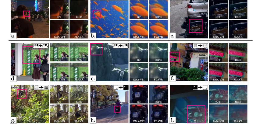
Figure 3: Examples from the LAVIB benchmark and OOD test sets (best viewed digitally). Zoomed regions on the right of each frame show interpolations with RIFE, EMA-VFI, and FLAVR. The top row shows results for videos from the benchmark test split. The bottom two rows are video frames from test splits from OOD challenges. The challenge is denoted at the top right of each ground truth frame. The ground truth is shown as a reference at the top left of the zoomed-in region grid.

5.4 Qualitative results

Fig. 3 shows interpolated frames from the LAVIB test sets. Frame regions from videos of the LAVIB benchmark interpolated with RIFE, EMA-VFI, and FLAVR are shown in the top row (a-c). Regions shown vary by size and reconstruction error. LAVIB is challenging for current VFI methods as they cannot fully interpolate all parts of objects (b) or fine details (c). For OOD challenges models also struggle to correctly interpolate the high contrast between objects and backgrounds (e,f,h), distinct patterns (d), and details or objects (g,i). Further qualitative results are provided in §A5-0.

6 Conclusions

This paper introduces LAVIB, a large-scale general-purpose dataset and benchmark for VFI. LAVIB consists of 283,484 clips collected from 4K videos at 60fps with metrics computed per video specific to motions, sharpness, contrast, and luminance. With the release of the videos and the OOD challenges splits, LAVIB can be used as a robust benchmark and allow the community to investigate VFI under a diverse range of video settings, captured with different equipment, and across various domains.

LAVIB: A Large-scale Video Interpolation Benchmark – Appendix

Table A1: Vocabulary of search terms. Terms are grouped to five main types including location, activities, weather, misc, and camera types. Search queries are the combination of multiple terms with an additional ‘4K’.

Location			Activities		Weather	Misc	Camera types
city	region	country	sports	actions
[Amsterdam, Athens, Boston, Buenos Aires, Doha, Dubai, Istanbul, Lagos, Las Vegas, London, Los Angeles, Manchester, Mexico City, Miami, Montreal, New York, Paris, Perth, Porto, Rio de Janeiro, Seoul, Shanghai, Singapore, Tokyo, Venice, Vienna]	[Atlantic, California, Caribbean, England, Indian Ocean, Scandinavia, Sedona, Sicily, South East]	[Australia, Brazil, Bulgaria, Cambodia, Canada, China, Costa Rica, France, Germany, Iceland, India, Japan, Morocco, Mexico, Mongolia, Namibia, New Zealand, Nigeria, Russia, South Africa, Spain, Thailand]	[climbing, playing football, rafting, skating, skiing, snorkeling, snowboarding, tennis training]	[bike ride, car ride, dancing, exploration, walking]	[cloudy, overcast, rainy, snowing, sunny]	[Dolby Vision, PS5, animals, birds, flowers, forest, insects, marinelife, metro, mountains, ocean view, park, shoreline, car, underwater, wildlife, windmills]	[Blackmagic PCC 4K, Canon 5D Mark III, Canon EOS C200B, Canon EOS R6, DJI Inspire2, DJI OM4, DJI Osmo Pocket, GOPRO HERO10 Black, GOPRO HERO8 Black, GOPRO HERO9, GOPRO Max 360, Note 10 plus, RED RAVEN 4.5K, Samsung Galaxy, Sony A6700, Sony A7C, Yi 4K+, iPhone 12 Pro, iPhone 13 Pro]

A1-0 Vocabulary

The core component for creating search terms from the vocabulary is either a location, an activity, or specific objects/settings relevant to videos. Locations and activities include two levels of hierarchies. The structure of search terms changes based on the selected sub-group.

Location. The city subgroup is combined with a specific set of actions {bike ride, car ride, exploration, walking}. Weather conditions are added randomly to 1/3 of the search terms and camera types are added in 1/10, e.g.; ‘Amsterdam bike ride rainy GOPRO HERO10 Black 4K’. It was seen that camera-type prompts can return results more relevant to the camera (e.g. reviews) that are less relevant to the rest of the term searched. Thus, the probability of including camera types is kept low. For the region and country subgroups, prompts only include keywords such as ‘best of’ or ‘scenic’ as actions are less relevant when the locations are broad.

Activities. Two activity categories are defined as motion variances, which present an important challenge in VFI. The sports subgroup primarily includes videos with fast-moving people/objects or camera motion. Specific terms are combined for the following sports; climbing, rafting, skiing, and snowboarding are combined with any of the {forest, mountains}, snorkeling is combined with {marinelife, shoreline, underwater}, and tennis training is combined with {park}. This results in search items such as; ‘snowboarding mountain 4K’. The action subgroup is only used in combination with locations.

Misc. In addition to locations and activities, miscellaneous search terms are included to diversify search queries further. These terms are primarily combined with equipment to form queries; e.g. ‘ocean view Yi 4K+ 4K’.

Algorithm 1 DUPLEX video selection

Input: dataset $\mathcal{D}$, sets { train, val, test }
      Output: dataset splits: $\{\mathcal{D}_{\text{train}},\mathcal{D}_{\text{val}},\mathcal{D}_{\text{test}}\}$

1:for $\text{set}\_\text{i}\;\in\{\text{train},\text{val},\text{test}\}$ do

2:     $\mathbf{s}\leftarrow\text{max}(\{\|\mathbf{x}_{j}-\mathbf{x}_{k}^{T}\|_{2}\})$ where $\mathbf{x}_{j},\mathbf{x}_{k}$ are metrics for videos $j,k$ within $\mathcal{D}$.

3:     $\mathcal{D}_{\text{set}\_\text{i}}\leftarrow\{j,k\}$

4:     $\mathcal{D}\leftarrow\mathcal{D}\setminus\{j,k\}$

5:end for

6:for $\text{set}\_\text{idx}\;\in\{tr,v,ts\}$ do

7:     for $i\;\in\{3,\text{set}\_\text{idx}\}$ do

8:         $\mathbf{s}_{i}\leftarrow\text{max}(\{\|\mathbf{x}_{l}-\mathcal{D}_{\text{set}\_\text{idx}}[-1]^{T}\|_{2}\})$ where $\mathbf{x}_{l}$ is a video in $\mathcal{D}$.

9:         $\mathcal{D}_{\text{set}\_\text{idx}}\leftarrow\mathcal{D}_{\text{set}\_\text{idx}}\cup\{\mathbf{x}_{l}\}$

10:         $\mathcal{D}\leftarrow\mathcal{D}\setminus\{\mathbf{x}_{l}\}$

11:     end for

12:end for

A2-0 Video sorting

For the benchmark, each split should have similar video metric distributions. Due to the multi-dimensionality and high variance across metrics, DUPLEX is used to calibrate dataset split sampling. DUPLEX uses the L2 distance across video metrics when creating train/val/test splits. For each set, the algorithm discovers the two most distant videos given their AFM, ALV, ARMS, and ARL metrics. It then iteratively samples videos that maximize the distance to previously sampled videos. This is done iteratively until the size condition for the split is met. Algorithm 1 provides a programmatic view of DUPLEX sampling.

A3-0 Detailed training settings

All training experiments are done with the codebases provided by the authors with $2\times$ Nvidia L40 with an average training time of 2 days per model. Computational settings for each model are reported in Tables A4, A4 and A4.

Table A2: RIFE settings

Parameter	value
batch size	64
optimizer	AdamW
weight decay	1e${}^{\!\!-6}$
learning rate	1e${}^{\!\!-4}$
learning scheduler	Step
additional params	beta1=0.9 beta2=0.99

Table A3: EMA-VFI settings.

Parameter	value
batch size	64
optimizer	AdamW
weight decay	1e${}^{\!\!-4}$
learning rate	1e${}^{\!\!-4}$
learning scheduler	Warmup
additional params	beta1=0.9 beta2=0.99

Table A4: FLAVR settings

Parameter	value
batch size	64
optimizer	Adam
weight decay	1e${}^{\!\!-6}$
learning rate	5e${}^{\!\!-3}$
learning scheduler	Step
additional params	beta1=0.9 beta2=0.99

A4-0 Ablations

Supplementary to the main results in §5 ablations are performed with FLAVR for variations in train set sizes for both benchmark and OOD challenges.

Benchmarks over reduced training set sizes. Section A4-0 presents val and test set results with reductions in the training set sizes. At each reduction setting, clips are dropped randomly. Performance drops significantly for both validation and test sets as the size of the training set decreases with an average -4.12 and -0.086 PSNR/SSIM.

Table A5: Val and test set results when training on different portions of the train set. full denotes that the entire train set from LAVIB is retained for training. Best results per split are in bold.

LAVIB train %	val set			test set
	PSNR$\uparrow$	SSIM$\uparrow$	LPIPS$\downarrow$	PSNR$\uparrow$	SSIM$\uparrow$	LPIPS$\downarrow$
20%	29.43	0.895	8.257e${}^{\!\!-2}$	29.48	0.894	8.472e${}^{\!\!-2}$
40%	31.68	0.960	4.108e${}^{\!\!-2}$	31.63	0.958	4.241e${}^{\!\!-2}$
60%	32.64	0.970	3.566e${}^{\!\!-2}$	32.50	0.967	3.835e${}^{\!\!-2}$
80%	33.36	0.975	2.971e${}^{\!\!-2}$	33.19	0.973	3.064e${}^{\!\!-2}$
full	33.72	0.981	2.515e${}^{\!\!-2}$	33.44	0.981	2.934e${}^{\!\!-2}$

Figure A1-0: Test PSNR/SSIM over train sizes. In ratios $<1.0\%$ clips are removed. In ratios $>1.0\%$ clips are added from left-out segments.

Table A6: AFM OOD ablation results.

AFM sett.	Train % removed	PSNR$\uparrow$	SSIM$\uparrow$	LPIPS$\downarrow$
$\rightarrow$	- bottom 30%	29.45	0.912	5.637e${}^{\!\!-2}$
	- top 30 %	26.32	0.854	9.428e${}^{\!\!-2}$
	None	30.67	0.959	5.094e${}^{\!\!-2}$
$\rightarrow$	- bottom 30%	32.80	0.973	3.396e${}^{\!\!-2}$
	- top 30 %	35.32	0.987	1.503e${}^{\!\!-2}$
	None	35.66	0.991	1.342e${}^{\!\!-2}$

Table A7: ALV OOD ablation results.

ALV sett.	Train % removed	PSNR$\uparrow$	SSIM$\uparrow$	LPIPS$\downarrow$
$\rightarrow$	- bottom 30%	30.32	0.933	4.781e${}^{\!\!-2}$
	- top 30 %	28.54	0.905	5.567e${}^{\!\!-2}$
	None	31.78	0.962	2.942e${}^{\!\!-2}$
$\rightarrow$	- bottom 30%	31.24	0.958	4.396e${}^{\!\!-2}$
	- top 30 %	34.35	0.971	2.740e${}^{\!\!-2}$
	None	34.67	0.975	2.627e${}^{\!\!-2}$

Table A8: ARMS OOD ablation results.

ARMS sett.	Train % removed	PSNR$\uparrow$	SSIM$\uparrow$	LPIPS$\downarrow$
$\rightarrow$	- bottom 30%	32.87	0.977	2.683e${}^{\!\!-2}$
	- top 30 %	31.92	0.965	3.769e${}^{\!\!-2}$
	None	33.02	0.982	2.561e${}^{\!\!-2}$
$\rightarrow$	- bottom 30%	30.18	0.931	4.515e${}^{\!\!-2}$
	- top 30 %	30.74	0.973	3.327e${}^{\!\!-2}$
	None	31.11	0.977	3.024e${}^{\!\!-2}$

Table A9: ARL OOD ablation results.

ARL sett.	Train % removed	PSNR$\uparrow$	SSIM$\uparrow$	LPIPS$\downarrow$
$\rightarrow$	- bottom 30%	32.76	0.973	2.806e${}^{\!\!-2}$
	- top 30 %	32.15	0.961	3.315e${}^{\!\!-2}$
	None	33.97	0.980	2.543e${}^{\!\!-2}$
$\rightarrow$	- bottom 30%	34.06	0.972	2.763e${}^{\!\!-2}$
	- top 30 %	33.67	0.970	3.457e${}^{\!\!-2}$
	None	34.20	0.976	2.875e${}^{\!\!-2}$

Performance over varying size. Motivated by the performance reductions observed with decreases in the train set size in Section A4-0, Fig. A1-0 presents PSNR/SSIM performance when an additional number of clips is retained during the selection progress. Clips are added by relaxing the threshold values. Although the performance improvements observed when including more clips in training in small ratios are significant, this is not retraced with further increases in the size of the current dataset. This shows that the selection process for LAVIB enables the creation of a diverse dataset.

OOD over reduced train set sizes. Performance trends when removing the highest/lowest valued clips in OOD challenges given their metrics are reported in Table A9 and Table A9 for AFM and ALV. Similarly, Table A9 and Table A9 report results with training set reductions for ARMS and ARL. Across settings, the portions closer to the target domain; e.g. the top 30% for the low to high settings and bottom 30% for the high to low settings present the largest drop in performance when removed. In contrast, when portions of the data that are less similar to the target domain are removed the reductions in performance are marginal. This shows that VFI method trained on domain-specific videos cannot generalize as effectively.

A5-0 Qualitative

Fig. A2-0 presents predicted frames from each model on examples from the benchmark test set. Interpolated frames for AFM-, ALV-, ARMS-, and ARL-based OOD challenges are shown in Figs. A3-0, A4-0, A5-0 and A6-0. In all settings, models can only partially interpolate the unseen frames. The majority of the errors observed are related to high-motion low-contrast examples. In instances where motion blur is present in the ground truth; e.g row 2 Fig. A2-0, row 5 in Fig. A3-0, and rows 1,5, and 6 in Fig. A4-0, motion blur is exacerbated at the interpolated frames from all models. Models trained on settings where fine details are not visible such as low ARMS and low ARL only interpolate the general shapes of objects and structures as shown in rows 1 and 2 in Fig. A5-0 and rows 1–3 in Fig. A6-0.

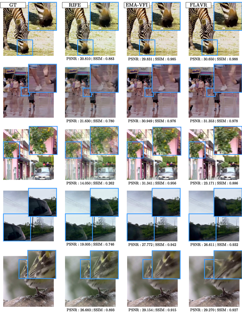
Figure A2-0: Examples from the LAVIB benchmark (best viewed digitally)

A6-0 Ethics and privacy

The introduced dataset primarily considers footage of landscapes, objects, nature, animals, and screen recordings. However, certain videos may include people. Scenes in which people appear are characterized by high camera motion, scene clutter, and partial visibility of faces briefly for a few seconds. Thus, it is believed that the risk of identification is low. In addition, the video segments from which the dataset is sourced are 1 second long, limiting the number of frames available. As videos are sourced from YouTube a list of the links to the original videos is also provided.

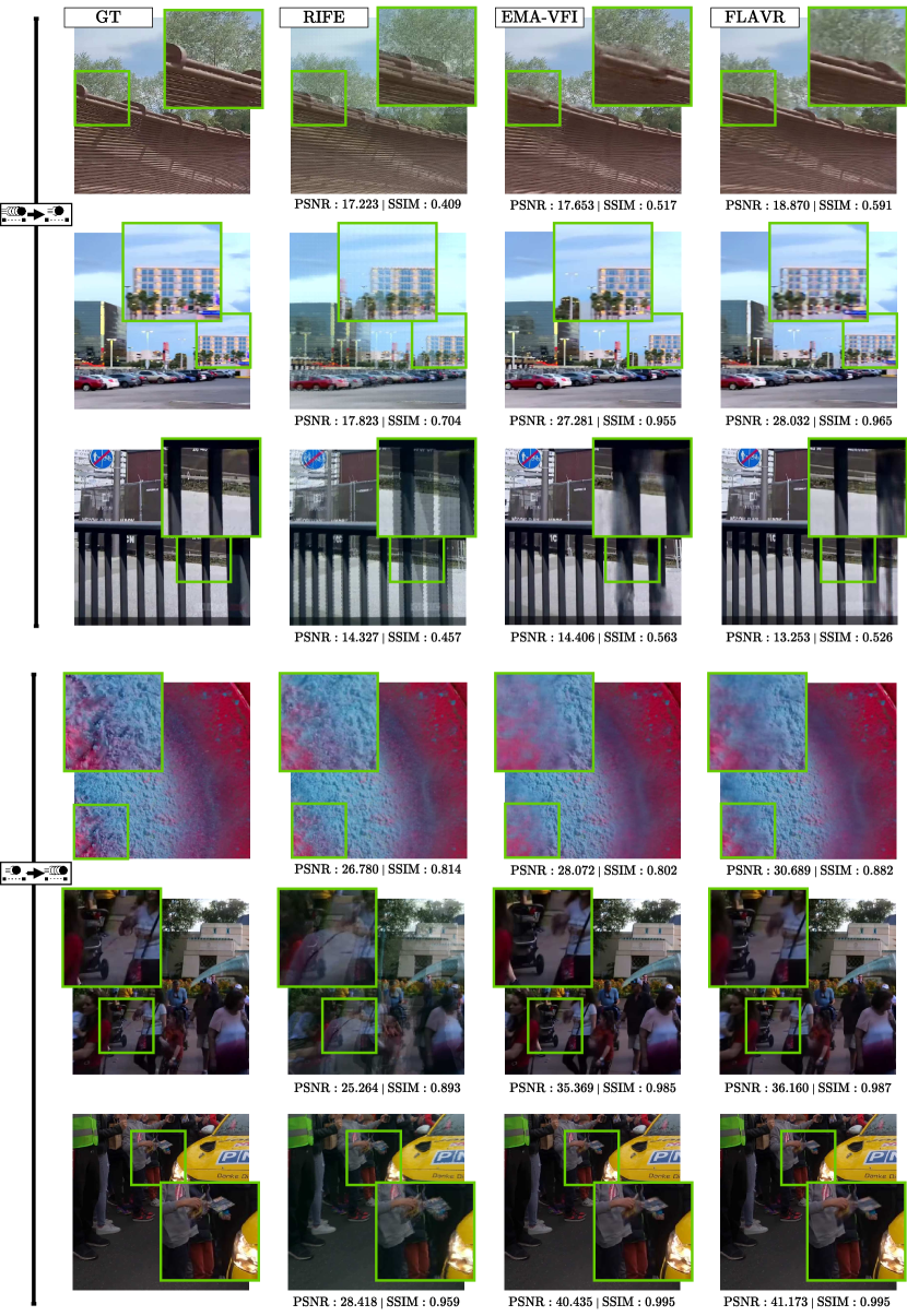
Figure A3-0: Examples of AFM OOD challenges (best viewed digitally)

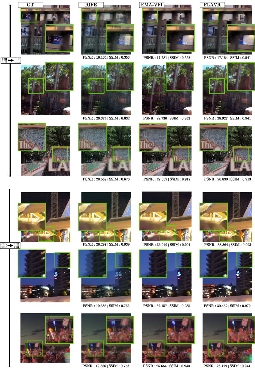
Figure A4-0: Examples of ALV OOD challenges (best viewed digitally)

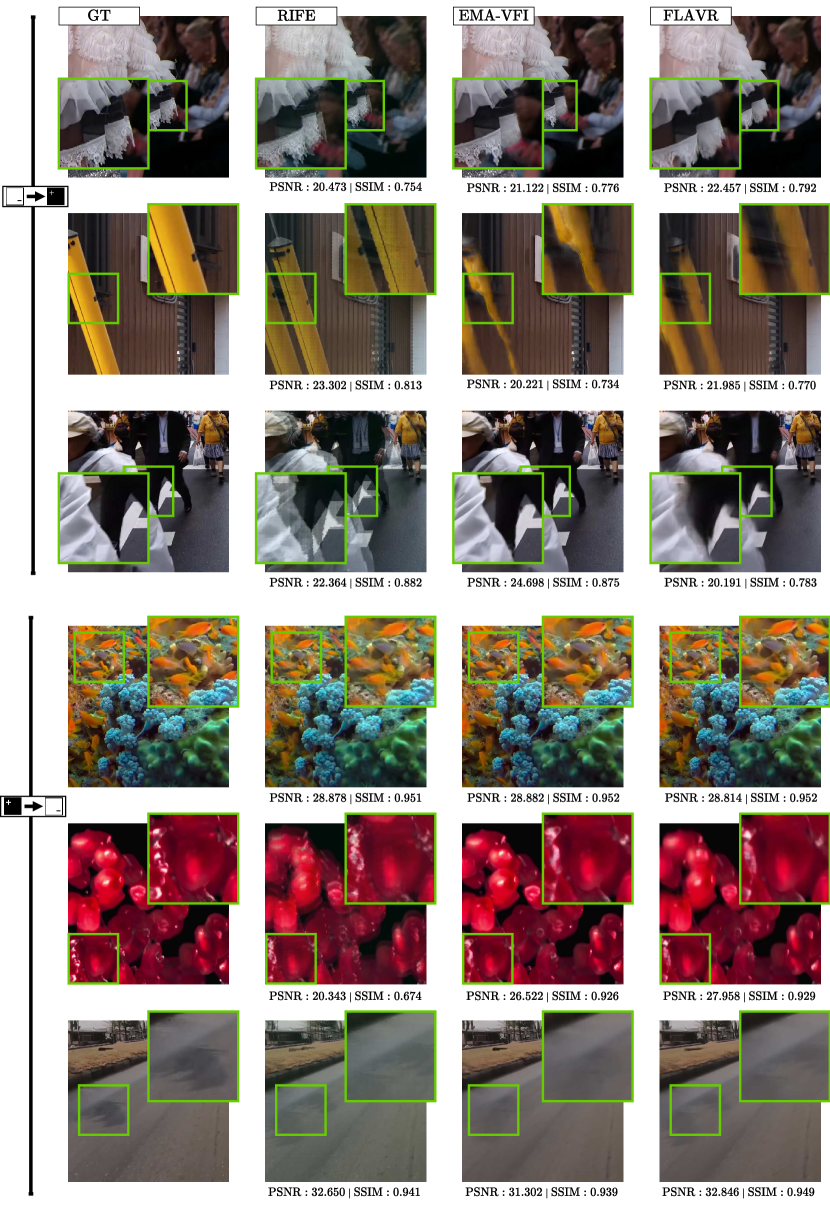
Figure A5-0: Examples of ARMS OOD challenges (best viewed digitally)

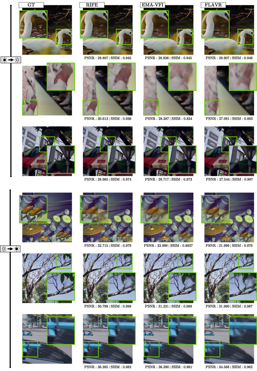
Figure A6-0: Examples of ARL OOD challenges (best viewed digitally)

References

- [1] Simon Baker, Daniel Scharstein, James P Lewis, Stefan Roth, Michael J Black, and Richard Szeliski. A database and evaluation methodology for optical flow. IJCV, pages 1–31, 2011.
- [2] Wenbo Bao, Wei-Sheng Lai, Chao Ma, Xiaoyun Zhang, Zhiyong Gao, and Ming-Hsuan Yang. Depth-aware video frame interpolation. In CVPR, pages 3703–3712, 2019.
- [3] AC Bovik, R Soundararajan, and Christos Bampis. On the robust performance of the st-rred video quality predictor, 2017.
- [4] Kelvin CK Chan, Shangchen Zhou, Xiangyu Xu, and Chen Change Loy. Basicvsr++: Improving video super-resolution with enhanced propagation and alignment. In CVPR, pages 5972–5981, 2022.
- [5] Angel X Chang, Thomas Funkhouser, Leonidas Guibas, Pat Hanrahan, Qixing Huang, Zimo Li, Silvio Savarese, Manolis Savva, Shuran Song, Hao Su, et al. Shapenet: An information-rich 3d model repository. arXiv preprint arXiv:1512.03012, 2015.
- [6] Myungsub Choi, Heewon Kim, Bohyung Han, Ning Xu, and Kyoung Mu Lee. Channel attention is all you need for video frame interpolation. In AAAI, pages 10663–10671, 2020.
- [7] Steffen Czolbe, Oswin Krause, Ingemar Cox, and Christian Igel. A loss function for generative neural networks based on watson’s perceptual model. NeurIPS, pages 2051–2061, 2020.
- [8] Keyan Ding, Kede Ma, Shiqi Wang, and Eero P Simoncelli. Image quality assessment: Unifying structure and texture similarity. TPAMI, pages 2567–2581, 2020.
- [9] Tianyu Ding, Luming Liang, Zhihui Zhu, and Ilya Zharkov. Cdfi: Compression-driven network design for frame interpolation. In CVPR, pages 8001–8011, 2021.
- [10] Christoph Feichtenhofer, Yanghao Li, Kaiming He, et al. Masked autoencoders as spatiotemporal learners. NeurIPS, pages 35946–35958, 2022.
- [11] Qiqi Hou, Abhijay Ghildyal, and Feng Liu. A perceptual quality metric for video frame interpolation. In ECCV, pages 234–253, 2022.
- [12] Mengshun Hu, Kui Jiang, Zhixiang Nie, and Zheng Wang. You only align once: Bidirectional interaction for spatial-temporal video super-resolution. In ACM-MM, pages 847–855, 2022.
- [13] Cong Huang, Jiahao Li, Bin Li, Dong Liu, and Yan Lu. Neural compression-based feature learning for video restoration. In CVPR, pages 5872–5881, 2022.
- [14] Zhaoyang Huang, Xiaoyu Shi, Chao Zhang, Qiang Wang, Ka Chun Cheung, Hongwei Qin, Jifeng Dai, and Hongsheng Li. Flowformer: A transformer architecture for optical flow. In ECCV, pages 668–685, 2022.
- [15] Zhewei Huang, Tianyuan Zhang, Wen Heng, Boxin Shi, and Shuchang Zhou. Real-time intermediate flow estimation for video frame interpolation. In ECCV, pages 624–642, 2022.
- [16] Takashi Isobe, Xu Jia, Xin Tao, Changlin Li, Ruihuang Li, Yongjie Shi, Jing Mu, Huchuan Lu, and Yu-Wing Tai. Look back and forth: Video super-resolution with explicit temporal difference modeling. In CVPR, pages 17411–17420, 2022.
- [17] Xiaozhong Ji, Yun Cao, Ying Tai, Chengjie Wang, Jilin Li, and Feiyue Huang. Real-world super-resolution via kernel estimation and noise injection. In CVPRw, pages 466–467, 2020.
- [18] Huaizu Jiang, Deqing Sun, Varun Jampani, Ming-Hsuan Yang, Erik Learned-Miller, and Jan Kautz. Super slomo: High quality estimation of multiple intermediate frames for video interpolation. In CVPR, pages 9000–9008, 2018.
- [19] Meiguang Jin, Zhe Hu, and Paolo Favaro. Learning to extract flawless slow motion from blurry videos. In CVPR, pages 8112–8121, 2019.
- [20] Xin Jin, Longhai Wu, Jie Chen, Youxin Chen, Jayoon Koo, and Cheul-hee Hahm. A unified pyramid recurrent network for video frame interpolation. In CVPR, pages 1578–1587, 2023.
- [21] Younghyun Jo, Seoung Wug Oh, Jaeyeon Kang, and Seon Joo Kim. Deep video super-resolution network using dynamic upsampling filters without explicit motion compensation. In CVPR, pages 3224–3232, 2018.
- [22] Tarun Kalluri, Deepak Pathak, Manmohan Chandraker, and Du Tran. Flavr: Flow-agnostic video representations for fast frame interpolation. In WACV, pages 2071–2082, 2023.
- [23] Andrej Karpathy, George Toderici, Sanketh Shetty, Thomas Leung, Rahul Sukthankar, and Li Fei-Fei. Large-scale video classification with convolutional neural networks. In CVPR, pages 1725–1732, 2014.
- [24] Taewoo Kim, Yujeong Chae, Hyun-Kurl Jang, and Kuk-Jin Yoon. Event-based video frame interpolation with cross-modal asymmetric bidirectional motion fields. In CVPR, pages 18032–18042, 2023.
- [25] Matej Kristan, Jiri Matas, Aleš Leonardis, Tomáš Vojíř, Roman Pflugfelder, Gustavo Fernandez, Georg Nebehay, Fatih Porikli, and Luka Čehovin. A novel performance evaluation methodology for single-target trackers. TPAMI, pages 2137–2155, 2016.
- [26] Orest Kupyn, Tetiana Martyniuk, Junru Wu, and Zhangyang Wang. Deblurgan-v2: Deblurring (orders-of-magnitude) faster and better. In ICCV, pages 8878–8887, 2019.
- [27] Dingquan Li, Tingting Jiang, and Ming Jiang. Quality assessment of in-the-wild videos. In ACM-MM, pages 2351–2359, 2019.
- [28] Haopeng Li, Yuan Yuan, and Qi Wang. Video frame interpolation via residue refinement. In ICASSP, pages 2613–2617, 2020.
- [29] Yinxiao Li, Pengchong Jin, Feng Yang, Ce Liu, Ming-Hsuan Yang, and Peyman Milanfar. Comisr: Compression-informed video super-resolution. In ICCV, pages 2543–2552, 2021.
- [30] Jingyun Liang, Jiezhang Cao, Yuchen Fan, Kai Zhang, Rakesh Ranjan, Yawei Li, Radu Timofte, and Luc Van Gool. Vrt: A video restoration transformer. T-IP, pages 2171–2182, 2024.
- [31] Jingyun Liang, Yuchen Fan, Xiaoyu Xiang, Rakesh Ranjan, Eddy Ilg, Simon Green, Jiezhang Cao, Kai Zhang, Radu Timofte, and Luc V Gool. Recurrent video restoration transformer with guided deformable attention. NeurIPS, pages 378–393, 2022.
- [32] Ce Liu and Deqing Sun. On bayesian adaptive video super resolution. TPAMI, pages 346–360, 2013.
- [33] Arthur B Markman and Dedre Gentner. Nonintentional similarity processing. The new unconscious, pages 107–137, 2005.
- [34] Reece Mazade, Jianzhong Jin, Hamed Rahimi-Nasrabadi, Sohrab Najafian, Carmen Pons, and Jose-Manuel Alonso. Cortical mechanisms of visual brightness. Cell reports, pages 111438–111438, 2022.
- [35] Christopher Montgomery and H Lars. Xiph. org video test media (derf’s collection). Online, https://media. xiph. org/video/derf, 6, 1994.
- [36] Seungjun Nah, Sungyong Baik, Seokil Hong, Gyeongsik Moon, Sanghyun Son, Radu Timofte, and Kyoung Mu Lee. Ntire 2019 challenge on video deblurring and super-resolution: Dataset and study. In CVPRw, pages 1996–2005, 2019.
- [37] Seungjun Nah, Tae Hyun Kim, and Kyoung Mu Lee. Deep multi-scale convolutional neural network for dynamic scene deblurring. In CVPR, pages 3883–3891, 2017.
- [38] Simon Niklaus and Feng Liu. Softmax splatting for video frame interpolation. In CVPR, pages 5437–5446, 2020.
- [39] Simon Niklaus, Long Mai, and Feng Liu. Video frame interpolation via adaptive separable convolution. In ICCV, pages 261–270, 2017.
- [40] Avinash Paliwal, Andrii Tsarov, and Nima Khademi Kalantari. Implicit view-time interpolation of stereo videos using multi-plane disparities and non-uniform coordinates. In CVPR, pages 888–898, 2023.
- [41] Junheum Park, Chul Lee, and Chang-Su Kim. Asymmetric bilateral motion estimation for video frame interpolation. In ICCV, pages 14539–14548, 2021.
- [42] Eli Peli. Contrast in complex images. JOSA A, pages 2032–2040, 1990.
- [43] Federico Perazzi, Jordi Pont-Tuset, Brian McWilliams, Luc Van Gool, Markus Gross, and Alexander Sorkine-Hornung. A benchmark dataset and evaluation methodology for video object segmentation. In CVPR, pages 724–732, 2016.
- [44] Charles Poynton. Digital video and HD: Algorithms and Interfaces. Elsevier, 2012.
- [45] Hamed Rahimi-Nasrabadi, Veronica Moore-Stoll, Jia Tan, Stephen Dellostritto, JianZhong Jin, Mitchell W Dul, and Jose-Manuel Alonso. Luminance contrast shifts dominance balance between on and off pathways in human vision. Journal of Neuroscience, pages 993–1007, 2023.
- [46] Fitsum Reda, Janne Kontkanen, Eric Tabellion, Deqing Sun, Caroline Pantofaru, and Brian Curless. Film: Frame interpolation for large motion. In ECCV, pages 250–266, 2022.
- [47] Denys Rozumnyi, Martin R Oswald, Vittorio Ferrari, Jiri Matas, and Marc Pollefeys. Defmo: Deblurring and shape recovery of fast moving objects. In CVPR, pages 3456–3465, 2021.
- [48] Wentao Shangguan, Yu Sun, Weijie Gan, and Ulugbek S Kamilov. Learning cross-video neural representations for high-quality frame interpolation. In ECCV, pages 511–528, 2022.
- [49] Dev Yashpal Sheth, Sreyas Mohan, Joshua L Vincent, Ramon Manzorro, Peter A Crozier, Mitesh M Khapra, Eero P Simoncelli, and Carlos Fernandez-Granda. Unsupervised deep video denoising. In ICCV, pages 1759–1768, 2021.
- [50] Shuwei Shi, Jinjin Gu, Liangbin Xie, Xintao Wang, Yujiu Yang, and Chao Dong. Rethinking alignment in video super-resolution transformers. NeurIPS, pages 36081–36093, 2022.
- [51] Hyeonjun Sim, Jihyong Oh, and Munchurl Kim. Xvfi: extreme video frame interpolation. In ICCV, pages 14489–14498, 2021.
- [52] Li Siyao, Shiyu Zhao, Weijiang Yu, Wenxiu Sun, Dimitris Metaxas, Chen Change Loy, and Ziwei Liu. Deep animation video interpolation in the wild. In CVPR, pages 6587–6595, 2021.
- [53] Ronald D Snee. Validation of regression models: methods and examples. Technometrics, pages 415–428, 1977.
- [54] Mingyang Song, Yang Zhang, and Tunç O Aydın. Tempformer: Temporally consistent transformer for video denoising. In ECCV, pages 481–496, 2022.
- [55] Khurram Soomro, Amir Roshan Zamir, and Mubarak Shah. Ucf101: A dataset of 101 human actions classes from videos in the wild. arXiv preprint arXiv:1212.0402, 2012.
- [56] Alexandros Stergiou and Ronald Poppe. Adapool: Exponential adaptive pooling for information-retaining downsampling. T-IP, pages 251–266, 2022.
- [57] Shuochen Su, Mauricio Delbracio, Jue Wang, Guillermo Sapiro, Wolfgang Heidrich, and Oliver Wang. Deep video deblurring for hand-held cameras. In CVPR, pages 1279–1288, 2017.
- [58] Xin Tao, Hongyun Gao, Renjie Liao, Jue Wang, and Jiaya Jia. Detail-revealing deep video super-resolution. In ICCV, pages 4472–4480, 2017.
- [59] Matias Tassano, Julie Delon, and Thomas Veit. Dvdnet: A fast network for deep video denoising. In ICIP, pages 1805–1809, 2019.
- [60] Longguang Wang, Yulan Guo, Li Liu, Zaiping Lin, Xinpu Deng, and Wei An. Deep video super-resolution using hr optical flow estimation. T-IP, pages 4323–4336, 2020.
- [61] Zhou Wang, Alan C Bovik, Hamid R Sheikh, and Eero P Simoncelli. Image quality assessment: from error visibility to structural similarity. T-IP, pages 600–612, 2004.
- [62] Zhongyuan Wang, Peng Yi, Kui Jiang, Junjun Jiang, Zhen Han, Tao Lu, and Jiayi Ma. Multi-memory convolutional neural network for video super-resolution. T-IP, pages 2530–2544, 2018.
- [63] Dan Xu, Andrea Vedaldi, and Joao F Henriques. Moving slam: Fully unsupervised deep learning in non-rigid scenes. In IROS, pages 4611–4617, 2021.
- [64] Tianfan Xue, Baian Chen, Jiajun Wu, Donglai Wei, and William T Freeman. Video enhancement with task-oriented flow. IJCV, pages 1106–1125, 2019.
- [65] Peng Yi, Zhongyuan Wang, Kui Jiang, Junjun Jiang, and Jiayi Ma. Progressive fusion video super-resolution network via exploiting non-local spatio-temporal correlations. In ICCV, pages 3106–3115, 2019.
- [66] Jun-Sang Yoo, Hongjae Lee, and Seung-Won Jung. Video object segmentation-aware video frame interpolation. In ICCV, pages 12322–12333, 2023.
- [67] Guozhen Zhang, Yuhan Zhu, Haonan Wang, Youxin Chen, Gangshan Wu, and Limin Wang. Extracting motion and appearance via inter-frame attention for efficient video frame interpolation. In CVPR, pages 5682–5692, 2023.
- [68] Richard Zhang, Phillip Isola, Alexei A Efros, Eli Shechtman, and Oliver Wang. The unreasonable effectiveness of deep features as a perceptual metric. In CVPR, pages 586–595, 2018.