Interior-Point-based $H_{2}$ Controller Synthesis for Compartmental Systems

Abstract

This paper addresses the problem of the optimal $H_{2}$ controller design for compartmental systems. In other words, we aim to enhance system robustness while maintaining the law of mass conservation. We perform a novel problem transformation and establish that the original problem is equivalent to an new optimization problem with a closed polyhedron constraint. Existing works have developed various first-order methods to tackle inequality constraints. However, the performance of the first-order method is limited in terms of convergence speed and precision, restricting its potential in practical applications. Therefore, developing a novel algorithm with fast speed and high precision is critical. In this paper, we reformulate the problem using log-barrier functions and introduce two separate approaches to address the problem: the first-order interior point method (FIPM) and the second-order interior point method (SIPM). We show they converge to a stationary point of the new problem. In addition, we propose an initialization method to guarantee the interior property of initial values. Finally, we compare FIPM and SIPM through a room temperature control example and show their pros and cons.

I Introduction

Compartmental systems refer to systems in which units, called compartments, interact with each other, and meanwhile obey the law of mass conservation. Such systems were first introduced in [1]. A more general introduction can be found in [2] and [3]. In many industrial systems with no interaction with the environment, the descriptor variables are not only non-negative but also their sum is non-increasing. For example, without the external supply, the total volume of material satisfies the law of mass conservation in a discrete-time compartmental flow model [4]. Besides, the air traffic network can be divided into many air centers with conservative inflows and outflows[5]. Similarly, the network that models the vehicles in the highway can also be modeled to be compartmental[6]. Compartmental systems are a special kind of positive systems that can easily be implemented in reality.

Recently, the $H_{2}$ and LQR control with the positive constraint have attracted many researchers in the control community. Deaecto and Geromel[7] proposed an iterative linear matrix inequality (ILMI) approach that can generate a solution sequence with non-increasing $H_{2}$ performance, thus guaranteeing convergence to a sub-optimal point. Furthermore, Ebihara et al. [8] derived the upper bound and the lower bound of the optimal $H_{2}$ performance using semidefinite programming (SDP). Recently, Yang et al.[9] proposed a projection-based LQR control of positive systems and showed it outperforms the methods in [7]. As a special kind of positive systems, some results have been obtained on the stabilization of compartmental systems recently. Valcher and Zorzan[10, 11] thoroughly studied the stabilization of compartmental systems and provided feasible approaches to find the stabilized controller under different circumstances. In our recent work [12], the optimal $H_{2}$ control of continuous-time compartmental systems was discussed, but the algorithm is first-order without convergence guarantee. Meanwhile, the discrete-time case is still missing, and more efficient computation methods, including higher-order algorithms, remain to be developed. This motivates our research in this paper.

Extensive research has been conducted on the LQR and $H_{2}$ controller synthesis subject to structural constraints. Chanekar et al.[13] considered adding a lower bound and an upper bound on the controller. In addition, Wu [14] considered general structural constraints, i.e., the constraints are mixed with equality, inequality, and scaling. Furthermore, Wu [15] considered the mixed $H_{2}$/$H_{\infty}$ control where the $H_{\infty}$ is kept within a threshold. However, all these works only relied on the first-order method and did not consider the Hessian information. Fatkhullin and Polyak [16] proposed a Hessian operator acting in a specific direction. However, this method can only be applied to accelerate the line search. The main algorithm is still a first-order method. Recently, Cheng et al.[17] proposed a second-order method in the continuous case, but only equality constraints are considered. To the best of our knowledge, no existing work considered the second-order method on the design of controllers subject to compartmental constraints, a kind of linear inequality constraint that cannot be tackled by the aforementioned methods.

The contributions of this paper are multifolds. First, we propose a novel problem transformation technique and establish an equivalent optimization problem with a closed polyhedron feasible region. Second, we characterize the optimality conditions of the reformulated problem via the KKT conditions. Third, for the first time, we introduce the interior point method with the log-barrier function and propose the first-order interior point method (FIPM) along with a novel second-order interior point method (SIPM) using damped Newton’s method. We also develop a procedure to determine a strictly feasible controller for initialization. Finally, we conduct thorough numerical simulations to compare the performance of the FIPM and the SIPM in various system dimensions.

This paper is organized as follows. In Section II, some preliminaries on compartmental systems and $H_{2}$ performance are provided and the problem is formulated. In Section III, we conduct the problem transformation and present the first-order optimality conditions. In Section IV, we introduce the log-barrier term and propose the FIPM with guaranteed convergence. In Section V, we provide detailed derivations for the Hessian matrix of the $H_{2}$ objective function and the log-barrier term, propose a Hessian modification method to guarantee descending and present the SIPM with guaranteed convergence. In Section VI, we discuss the initialization of a strictly feasible controller. In Section VII, several numerical simulations on room temperature control are provided to compare the performance of FIPM and SIPM in different system scales. The paper is concluded in Section VIII.

Notations: The notation $R^{m\times n}$ denotes the set of all real matrices of size $m\times n$, and $R^{m\times n}_{+}$ denotes the set of real matrices with non-negative entries of size $m\times n$. For a matrix $X$, $X^{T}$ denotes its transpose, $X^{H}$ denotes its conjugate transpose, $X^{k}$ denotes its $k^{th}$ power, $\{X^{(k)}\}$ denotes a matrix sequence, $Tr(X)$ denotes its trace, $X_{ij}$ denotes its element at $i$-th row and $j$-th column. The notation $\partial$ denotes the boundary of a set. The identity matrix and the zero matrix are denoted by $I$ and 0, with dimensions labeled using subscripts if necessary. The notation $X>0$ (or $X\geq 0$) means each entry of matrix $X$ is positive (or non-negative). The notation $X\succ 0$ (or $X\succeq 0$) means matrix $X$ is positive definite (or semidefinite). We use $\mathbf{0}$ and $\mathbf{1}$ to denote the all-zeros column vectors and all-ones column vectors with compatible dimensions. $\mathrm{diag}(a_{1},a_{2},\ldots,a_{n})$ represents a diagonal matrix with $a_{i},\forall{i}=1,2,\ldots,n$ on its diagonal. Similarly, $\mathrm{blkdiag}(A_{1},A_{2},\ldots,A_{n})$ represents putting $A_{i},\forall{i}=1,2,\ldots,n$ in a block diagonal way. $\left[A_{1}|A_{2}|\ldots|A_{n}\right]$ represents organizing $A_{i},\forall{i}=1,2,\ldots,n$ in one row. The operator $\otimes$ represents the Kronecker product. $(\cdot)^{*}$ represents the adjoint operator. $\circ$ represents the Hadamard operator. The operator $\mathrm{vec}(\cdot)$ represents the vectorization operation that expands a matrix by column into a column vector. $\mathrm{mat}(\cdot)$ represents the matrixization operation that reorganizes a column vector into a matrix with appropriate dimensions by column.

II Preliminaries

II-A Compartmental Systems

We can use a non-negative matrix $A\in R^{n\times n}$ to describe a digraph $\mathcal{D}(A)=\{\mathcal{V},\mathcal{E}\}$, where $\mathcal{V}=\{1,...,n\}$ is the set of vertices and $\mathcal{E}$ is the set of edges. There is an arc $(i,j)\in\mathcal{E}$ from $i$ to $j$ if and only if $A_{ji}>0$, where $A_{ji}$ is called the weight of the arc. A sequence of nodes $i_{1}\rightarrow i_{2}\rightarrow\cdots\rightarrow i_{n}$ is called a path if $(i_{1},i_{2})\in\mathcal{E},\ldots,(i_{n-1},i_{n})\in\mathcal{E}$. We say $j$ is accessible from $i$ if there is a path from $i$ to $j$, or equivalently, $A^{l}_{ji}>0$ for some $l$. Two different nodes $i$ and $j$ communicate if each of them is accessible from the other. Therefore, we can divide $\mathcal{V}$ into communicating classes, say $C_{1},C_{2}\ldots C_{k}$. If there exists $g\in C_{i}$ and $h\in C_{j}$ such that $g$ accesses $h$, then we say $C_{i}$ accesses $C_{j}$. Each $C_{i}$ accesses itself trivially. The digraph $\mathcal{D}(A)$ is strongly connected if every two nodes communicate with the other. Equivalently, there is only one communicating class $\mathcal{V}$. The digraph $\mathcal{D}(A)$ is strongly connected if and only if $A$ is irreducible.

A non-negative matrix with all of its columns sum no larger than 1 is called a compartmental matrix, i.e., $\mathbf{1}^{T}A\leq\mathbf{1}^{T}$. It is commonly used to describe flows between compartments. It can be understood that there is an outflow from each node to the others. If the outflow is more than the inflow, there must be a loss of material to the environment. Mathematically, we call node $i$ an outflow node if $\mathbf{1}^{T}Ae_{i}<1$. The node $j$ is said to be outflow-connected if there is a path from that node to an outflow node. Thus it is easy to conclude that a compartmental matrix is Schur if and only if every node is outflow-connected.

II-B $H_{2}$ Performance

Consider a discrete-time linear time-invariant (LTI) system

$$x_{k+1} =Ax_{k}+Bu_{k}+Gd_{k}$$ (1)

$$y_{k} =Cx_{k}+Du_{k}$$

where $x\in R^{n}$ is the state, $u\in R^{m}$ is the control, $d\in R^{n}$ is the exogenous disturbance, $y\in R^{r}$ is the controlled output. It is standard to assume that $(A,B)$ is stabilizable, $D^{T}C=0$ and $D^{T}D\succ 0$[18]. The system adopts static state-feedback control law

$$u_{k}=-Kx_{k}$$ (2)

where $K$ is the gain to be determined. Therefore, we can rewrite system (1) into following form

$$x_{k+1} =A_{K}x_{k}+Gd_{k}$$ (3)

$$y_{k} =C_{K}x_{k}$$

where $A_{K}=A-BK$ and $C_{K}=C-DK$. The close loop transfer function in $z$-domain from $d$ to $y$ is given by

$$T(z)=C_{K}(zI-A_{K})^{-1}G$$ (4)

It is known that the $H_{2}$ norm is bounded if the system is asymptotically stable. Therefore, the implicit domain of $K$ is $K\in\mathcal{F}$, where $\mathcal{F}\triangleq\{K\mid A-BK~{}\text{is Schur stable}\}$. The $H_{2}$ norm for a stable transfer function $T(z)$ is defined by

$$||T(z)||_{2}=\sqrt{\frac{1}{2\pi}\int^{\pi}_{-\pi}Tr(T(e^{-j\omega})^{H}T(e^{j\omega}))d\omega}$$ (5)

By defining $J(K)\triangleq||T(z)||^{2}_{2}$ as the objective function to be optimized, it is well known [19] that we can evaluate $J(K)$ as follows

$$J(K)=Tr(G^{T}XG)$$ (6)

where $X\succeq 0$ is the unique solution to

$$A_{K}^{T}XA_{K}-X+C_{K}^{T}C_{K}=0$$ (7)

II-C Problem Formulation

In this paper, we are interested in the optimal static state-feedback controller synthesis under $H_{2}$ performance for compartmental systems. The problem is formulated below.

Problem DHSCCS (Design of $H_{2}$ Static state-feedback Controller for Compartmental Systems): Consider the discrete-time LTI system in (1), design a static state-feedback controller in (2) such that the square of $H_{2}$ norm of the transfer function, as defined in (6), is minimized, and meanwhile the closed-loop system is both Schur stable and compartmental.

Remark 1

Intuitively, this problem is to find a $H_{2}$ static state-feedback controller that preserves the system’s physical property, i.e., the flow conservation law of the compartmental systems, and meanwhile enhances the system’s robustness against external disturbance. The main difficulty of this problem lies in three parts. First, the interior-point method requires a strictly feasible initial point. However, it is challenging to initialize a controller to make the system Schur and compartmental. Second, the $H_{2}$ performance is generally a non-convex function concerning $K$. Third, it is difficult for the system to simultaneously maintain Schur and compartmental. In this paper, we tackle these challenges from an optimization perspective using FIPM and SIPM.

III Basic Results

In this section, we will provide some basic results that are the prerequisites for further advanced discussions. First, we transform the original problem into an optimization problem with polyhedron constraints. Second, we derive the gradient of $J(K)$, which is essential for the first-order and the second-order methods. Finally, we depict the first-order optimal conditions via KKT conditions.

Theorem 1

Problem DHSCCS is equivalent to the following constrained optimization problem

$$\mathop{\min}_{K}J(K)$$ (8)

$${s.t.} \left\{\begin{array}[]{l}A_{K}\geq 0,\\ \mathbf{1}^{T}A_{K}\leq\mathbf{1}^{T}.\end{array}\right.$$

Proof: Since $A_{K}$ is required to be a compartmental matrix, which first has to be non-negative, the constraint $A_{K}\geq 0$ in (8) is trivial. If the compartmental matrix $A_{K}$ is Schur, every node is outflow connected. Thus, $\mathbf{1}^{T}A_{K}\leq\mathbf{1}^{T}$ and the equality does not hold. By denoting $\mathcal{S}\triangleq\{K\mid A_{K}\text{ is compartmental and Schur}\}$ and the set of compartmental gains $\mathcal{C}\triangleq\{K\mid A_{K}\geq 0\text{ and }\mathbf{1}^{T}A_{K}\leq\mathbf{1}^{T}\}$, it shows that $\mathcal{S}\subset\mathcal{C}$, $\mathcal{S}\subset\mathcal{F}$, and $\mathcal{C}-\mathcal{S}\subset\mathcal{\bar{F}}$, where $\mathcal{\bar{F}}$ denotes the complementary set of $\mathcal{F}$. Further note that as $K\rightarrow\partial\mathcal{F}$, $J(K)\rightarrow\infty$ due to the coercive property of $J(K)$ [20]. Therefore, from an optimization perspective, we can relax $\mathcal{S}$ to $\mathcal{C}$ without loss of generality, and thus the Problem DHSCCS is equivalent to (8). The proof is complete. $\hfill\square$

The differentiability of $J(K)$ is a well-known fact, shown by Levine and Athans[21]. In what follows, we characterize the gradient of $J(K)$ in the discrete-time $H_{2}$ control case.

Lemma 1

The gradient of $J(K)$ is given by

$$\nabla J(K)=2(B^{T}X(A-BK)-D^{T}DK)Y$$ (9)

where $Y\succeq 0$ is the unique solution to

$$A_{K}YA_{K}^{T}-Y=GG^{T}$$ (10)

Proof: Consider the increment of (7)

$$\begin{split}-dK^{T}B^{T}XA_{K}+A_{K}^{T}dXA_{K}-A_{K}^{T}XBdK-dX\\ -dK^{T}D^{T}C_{K}-C_{K}^{T}DdK=0\end{split}$$

Pre-multiplying both sides with $Y$ and take trace, we get

$$\begin{split}&dJ(K)=Tr(GG^{T}dX)=\\ &2Tr(B^{T}XA_{K}YdK^{T})+2Tr(D^{T}C_{K}YdK^{T})\end{split}$$

Reorganizing the terms, we obtain

$$dJ(K)=2Tr((B^{T}XA_{K}+D^{T}C_{K})YdK^{T})$$

and thus $\nabla J(K)=2(B^{T}XA_{K}-D^{T}DK)Y$ since $D^{T}C=0$. The proof is complete. $\hfill\square$

In this paper, we will solve the Problem DHSCCS from an optimization perspective. The Lagrangian function of the problem in (8) is constructed as follows.

$$L(K,Q)=J\left(K\right)-Tr\left(Q^{T}\left[\begin{array}[]{c}A-BK\\ \mathbf{1}^{T}-\mathbf{1}^{T}\left(A-BK\right)\\ \end{array}\right]\right)$$

where $Q$ is known as the Lagrangian multiplier. Due to the non-convexity, a global optimal solution is generally not available. Therefore, we will not use global optimal but local optimal instead. In what follows, we show that the necessary conditions for local optimality can be derived via the KKT conditions. According to the problem in (8), the inequality constraints are affine with respect to $K$, and thus it satisfies the linearity constraint qualification (LCQ). As a result, the strong duality holds, which means the duality gap is $0$. In other words, if $K^{*}$ is the local optimal solution to (8), there must exist a dual variable $Q^{*}$, known as KKT multiplier, such that the following KKT conditions hold.

$$\left\{\begin{array}[]{l}\nabla J\left(K^{*}\right)-\left[\begin{matrix}-B^{T}&B^{T}\mathbf{1}\\ \end{matrix}\right]Q^{*}=0\\ Q^{*}\geq 0\\ \left[\begin{array}[]{c}A-BK^{*}\\ \mathbf{1}^{T}-\mathbf{1}^{T}\left(A-BK^{*}\right)\\ \end{array}\right]\geq 0\\ Tr\left(Q^{*^{T}}\left[\begin{array}[]{c}A-BK^{*}\\ \mathbf{1}^{T}-\mathbf{1}^{T}\left(A-BK^{*}\right)\\ \end{array}\right]\right)=0\\ \end{array}\right.$$ (11)

Definition 1

$K\in\mathcal{F}$ is called a stationary point of problem (8) if it satisfies its KKT conditions in (11).

Remark 2

Notice that the local optimal solution to (8) must be a stationary point. However, a stationary point is not necessarily a local optimal point due to the existence of saddle points. Although getting sufficient conditions for local optimality is difficult, we can still eliminate points that are not local optimal or saddle. The stationary point is usually the highest pursuit for non-convex optimization problems.

IV First-Order Method

To the best of our knowledge, in $H_{2}$ control setting, most existing works deal with inequality constraints via dual methods, including the alternating direction method of multipliers (ADMM) and the augmented Lagrangian Method (ALM). However, although they have shown great performance, the convergence of these methods is not guaranteed in most non-convex cases. Other first-order methods such as projected gradient descent (PGD) can guarantee convergence, but the speed is rather slow. In this section, we propose a first-order interior point method (FIPM) to solve (8). There are two main advantages of this method: 1) It has been shown that FIPM has great performance in small-scale problems. 2) The solution in each iteration always exists in the feasible region, making it converge easier. We will show that FIPM converges to a

Input: $K^{(0)}$, $t^{(0)},\mu>1$

Output: $K^{*}$

Initialize $h=0$;

repeat

       - Initialize $k=0$;

       - $\hat{K}^{(k)}=K^{(h)}$;

       repeat

             - Calculate $\nabla_{K}JLBF(\hat{K}^{(k)},t^{(h)})$ by (14);

             - $\hat{K}^{(k+1)}=\hat{K}^{(k)}-s\nabla_{K}JLBF(\hat{K}^{(k)},t^{(h)})$, where $s$ is determined by Armijo rule [22];

             - $k=k+1$;

            

      until $||\nabla_{K}JLBF(\hat{K}^{(k)},t^{(h)}||<\epsilon_{1}$ or $\hat{K}^{(k)}=\hat{K}^{(k-1)}$;

      - $K^{(h+1)}=\hat{K}^{(k)}$;

       - $t^{(h+1)}=\mu t^{(h)}$;

       - $h=h+1$;

      

until  $||K^{(h+1)}-K^{(h)}||<\epsilon_{2}$;

return $K^{(h)}$.

Algorithm 1 FIPM for solving Problem DHSCCS

stationary point of the original problem. We first reformulate (8) into the following unconstrained problem.

$$\min_{K}J(K)-\cfrac{1}{t}\sum_{i,j}\mathrm{log}\left[\begin{array}[]{c}A-BK\\ \mathbf{1}^{T}-\mathbf{1}^{T}\left(A-BK\right)\\ \end{array}\right]_{ij}$$ (12)

where $t>0$ is the penalty parameter. The intuition for using the log-barrier function is that, as $t$ approaches $+\infty$, the log-barrier function will approximate an indicator function. Therefore, the solution $K$, as $t$ approaches $+\infty$, will converge to the solution of the original problem. Denote

$$\begin{split}&JLBF(K,t)=J(K)\\ &-\cfrac{1}{t}\sum_{i,j}\mathrm{log}\left(\left[\begin{array}[]{c}A\\ \mathbf{1}^{T}-\mathbf{1}^{T}A\\ \end{array}\right]+\left[\begin{array}[]{c}-B\\ \mathbf{1}^{T}B\\ \end{array}\right]K\right)_{ij}\end{split}$$ (13)

Since (12) is an unconstrained problem, and the object function is smooth, we use gradient descent to solve $\eqref{FIPM first order problem}$. The gradient of $JLBF$ is provided below. The full algorithm is shown in Algorithm 1.

$$\begin{split}&\nabla_{K}JLBF(K,t)=\nabla J(K)\\ &-\cfrac{1}{t}\cdot\left[\begin{matrix}-B^{T}&B^{T}\mathbf{1}\\ \end{matrix}\right]\cdot\left(\left[\begin{array}[]{c}A_{K}\\ \mathbf{1}^{T}-\mathbf{1}^{T}A_{K}\\ \end{array}\right]\right)^{\circ-1}\end{split}$$ (14)

Proposition 1

Algorithm 1 converges to a stationary point of problem (8).

Proof: Since $JLBF$ is continuous and coercive, by using Weierstrass’ Theorem, $JLBF$ attains the global minimum on its domain, and thus $JLBF$ is lower-bounded. Since we use gradient descent, we can obtain a non-increasing sequence, which guarantees the convergence of $\hat{K}^{(k)}$ for each penalty parameter $t^{(h)}$. In addition, the solution of FIPM at each iteration converges to the solution of the original problem (8) as $t\rightarrow\infty$. The proof of convergence is complete. Now we prove the stationary part. Since the algorithm is guaranteed to converge, we obtain

$$\begin{split}&\lim_{h\rightarrow\infty}\nabla_{K}JLBF(K^{(h+1)},t^{(h)})=\nabla J(K^{*})\\ &-\left[\begin{matrix}-B^{T}&B^{T}\mathbf{1}\\ \end{matrix}\right]\cdot Q^{*}\end{split}$$ (15)

where $Q^{*}=\lim_{h\rightarrow\infty}\cfrac{1}{t^{(h)}}\cdot\left(\left[\begin{array}[]{c}A_{K}^{(h+1)}\\ \mathbf{1}^{T}-\mathbf{1}^{T}A_{K}^{(h+1)}\\ \end{array}\right]\right)^{\circ-1}\geq 0$ and $A_{K}^{(h+1)}=A-BK^{(h+1)}$ because $K$ always exist in the feasible region and $t^{(h)}>0$. Hence, the first three conditions of (11) hold trivially. For the last condition, denote $S^{*}=\lim_{h\rightarrow\infty}\left[\begin{array}[]{c}A_{K}^{(h+1)}\\ \mathbf{1}^{T}-\mathbf{1}^{T}A_{K}^{(h+1)}\\ \end{array}\right]$. If there is an element $S^{*}_{ij}>0$, $Q^{*}_{ij}=0$ since $1/t^{(h)}$ will force it to $0$ as $h\rightarrow\infty$. Since the condition holds trivially, we do not need to consider $S^{*}_{ij}=0$. The proof is complete. $\hfill\square$

V Second-Order Method

Although the first-order method can converge to a stationary point, it suffers from a linear convergence rate, limiting its potential in practical situations. In this section, we propose a second-order interior point method (SIPM) to solve (8). The main difficulties lie in calculating the Hessian matrix for $J(K)$ and the second log-barrier term in (13). Since both terms are scalar functions concerning a matrix, their Hessian matrices should lie in a four-dimension space. To avoid discussing tensors, we propose vectorizing $K$ to guarantee their Hessian matrices are in two dimensions for the convenience of mathematical expressions. To facilitate discussions, denote

$$\varGamma X=-C_{K}^{T}C_{K}$$

$$\varGamma^{*}Y=GG^{T}$$

$$\varGamma_{mn}X=\partial_{K_{mn}}A_{K}^{T}XA_{K}+A_{K}^{T}X\partial_{K_{mn}}A_{K}$$

$$\varGamma_{mn}^{*}Y=\partial_{K_{mn}}A_{K}YA_{K}^{T}+A_{K}Y\partial_{K_{mn}}A_{K}^{T}$$

where we define the general Lyapunov operator $\varGamma:\mathbb{R}^{n\times n}\rightarrow\mathbb{R}^{n\times n}$ as $P\mapsto A_{K}^{T}PA_{K}-P$, and $K_{mn}$ denotes the entry on $m$-th row and $n$-th column of $K$. Furthermore, we have the inner product property $\left<\varGamma X,Y\right>=\left<X,\varGamma^{*}Y\right>$.

V-A Derivation of Hessian matrix

In this subsection, we explicitly compute the Hessian matrix of $J(K)$. We first express the Hessian matrix of $J(K)$ as the partial derivative of $\nabla J(K)$ for each entry of $K$, and then we obtain $\nabla_{\mathrm{vec}(K)}^{2}J(\mathrm{vec}(K))$, avoiding directly expressing $\nabla_{K}^{2}J(K)$. Similarly, we derive the gradient and Hessian matrix of the log barrier term in a vectorized sense.

Theorem 2

Consider the system (3), the partial derivative of $\nabla J(K)$ to each entry of $K$ can be obtained as

$$\begin{split}&\partial_{K}\partial_{K_{ij}}J=-2B^{T}\left[X^{ij}+\left(X^{ij}\right)^{T}\right]\left(A-BK\right)Y\\ &-2\left[B^{T}X\left(A-BK\right)-D^{T}DK\right]\left[Y^{ij}+\left(Y^{ij}\right)^{T}\right]\\ &-2\left[B^{T}XB+D^{T}D\right]S^{ij}Y\\ &+2B^{T}\left[Z^{ij}+\left(Z^{ij}\right)^{T}\right]\left(A-BK\right)Y\end{split}$$ (16)

where $S^{ij}$ denotes a sparse matrix with $1$ on $i$-th row and $j$-th column and $0$ on all other entries.

$$\varGamma X^{ij}=-\left(A-BK\right)^{T}XBS^{ij}$$

$$\varGamma^{*}Y^{ij}=-\left(A-BK\right)Y\left(S^{ij}\right)^{T}B^{T}$$

$$\varGamma Z^{ij}=-K^{T}D^{T}DS^{ij}$$

Proof: From (9), the gradient of $J$ with a single entry of $K$ can be expressed as

$$\begin{split}\partial_{K_{ij}}J&=2\left<B^{T}XA_{K}Y,S^{ij}\right>-2\left<D^{T}DKY,S^{ij}\right>\\ &=2\left<Y,A_{K}^{T}XBS^{ij}\right>-2\left<Y,K^{T}D^{T}DS^{ij}\right>\end{split}$$

Therefore, each entry of the Hessian matrix is

$$\begin{split}&\partial_{K_{mn}}\partial_{K_{ij}}J=2\left<\partial_{K_{mn}}Y,A_{K}^{T}XBS^{ij}\right>\\ &-2\left<Y,\left(BS^{mn}\right)^{T}XBS^{ij}\right>+2\left<Y,A_{K}^{T}\partial_{K_{mn}}XBS^{ij}\right>\\ &-2\left<\partial_{K_{mn}}Y,K^{T}D^{T}DS^{ij}\right>-2\left<Y,\left(S^{mn}\right)^{T}D^{T}DS^{ij}\right>\end{split}$$

By using the inner product property of $\varGamma$ and $\varGamma^{*}$, we have

$$\begin{split}&\partial_{K_{mn}}\partial_{K_{ij}}J=2\left<\varGamma^{*}_{mn}Y,\varGamma^{-1}\left[-\left(A-BK\right)^{T}XBS^{ij}\right]\right>\\ &-2\left<Y,A_{K}^{T}\left[\varGamma^{-1}\left(\varGamma_{mn}X\right)+\varGamma^{-1}\left(\partial_{K_{mn}}C_{K}^{T}C_{K}\right)\right]BS^{ij}\right>\\ &+2\left<Y,\left(-BS^{mn}H\right)^{T}XBS^{ij}\right>-2\left<Y,\left(S^{mn}\right)^{T}D^{T}DS^{ij}\right>\\ &-2\left<\varGamma^{*}_{mn}Y,\varGamma^{-1}\left(-K^{T}D^{T}DS^{ij}\right)\right>\\ \end{split}$$

From $\varGamma_{mn}X=\left(-BS^{mn}\right)^{T}XA_{K}+A_{K}^{T}X\left(-BS^{mn}\right)$ and $\varGamma^{*}_{mn}Y=\left(-BS^{mn}\right)YA_{K}^{T}+A_{K}Y\left(-BS^{mn}\right)^{T}$, we have

$$\begin{split}&\partial_{K_{mn}}\partial_{K_{ij}}J\\ &=2\left<\left(-BS^{mn}\right)YA_{K}^{T}+A_{K}Y\left(-BS^{mn}\right)^{T},X^{ij}\right>\\ &+2\left<Y^{ij},\left(-BS^{mn}\right)^{T}XA_{K}+A_{K}^{T}X\left(-BS^{mn}\right)\right>\\ &+\left<Y^{ij},\left(-DS^{mn}\right)^{T}C_{K}+C_{K}^{T}\left(-DS^{mn}\right)\right>\\ &+2\left<Y,\left(-BS^{mn}\right)^{T}XBS^{ij}\right>-2\left<Y,\left(S^{mn}\right)^{T}D^{T}DS^{ij}\right>\\ &-2\left<\left(-BS^{mn}\right)YA_{K}^{T}+A_{K}Y\left(-BS^{mn}\right)^{T},Z^{ij}\right>\\ \end{split}$$

By moving $S^{mn}$ and $(S^{mn})^{T}$ terms to one side, we have

$$\begin{split}&\partial_{K_{mn}}\partial_{K_{ij}}J=\\ &2\left<S^{mn},-B^{T}X^{ij}A_{K}Y\right>-2\left<\left(S^{mn}\right)^{T},YA_{K}^{T}X^{ij}B\right>\\ &-2\left<Y^{ij}A_{K}^{T}XB,\left(S^{mn}\right)^{T}\right>-2\left<B^{T}XA_{K}Y^{ij},S^{mn}\right>\\ &+2\left<-Y^{ij}C_{K}^{T}D,\left(S^{mn}\right)^{T}\right>-2\left<D^{T}C_{K}Y^{ij},S^{mn}\right>\\ &+2\left<-Y\left(S^{ij}\right)^{T}B^{T}XB,\left(S^{mn}\right)^{T}\right>\\ &+2\left<S^{mn},B^{T}Z^{ij}A_{K}Y\right>+2\left<\left(S^{mn}\right)^{T},YA_{K}^{T}Z^{ij}B\right>\\ &-2\left<Y\left(S^{ij}\right)^{T}D^{T}D,\left(S^{mn}\right)^{T}\right>\end{split}$$

Now we can extend $\partial_{K_{mn}}$ to $\partial_{K}$ by remove the $S^{mn}$ and $(S^{mn})^{T}$ terms. After reorganizing terms and combining similar terms we obtain (16). The proof is complete.$\hfill\square$

If we regard $K$ as $\mathrm{vec}(K)$ instead of a matrix, by leveraging Eq. 16, we can obtain the gradient and Hessian expression of $J(K)$ as

$$G_{J}(K)=\mathrm{vec}(\nabla J(K))$$ (18)

$$\begin{split}H_{J}(K)=&\left[\mathrm{vec}\left(\cfrac{\partial^{2}J}{\partial_{K_{11}}\partial_{K}}\right),\ldots,\mathrm{vec}\left(\cfrac{\partial^{2}J}{\partial_{K_{m1}}\partial_{K}}\right),\ldots\right.\\ &\left.\mathrm{vec}\left(\cfrac{\partial^{2}J}{\partial_{K_{1p}}\partial_{K}}\right),\ldots,\mathrm{vec}\left(\cfrac{\partial^{2}J}{\partial_{K_{mp}}\partial_{K}}\right)\right]\end{split}$$ (19)

After addressing the $J(K)$, we proceed to discuss the log-barrier term. Denote

$$LBF(K,t)=-\cfrac{1}{t}\sum_{i,j}\mathrm{log}\left[\begin{array}[]{c}A-BK\\ \mathbf{1}^{T}-\mathbf{1}^{T}\left(A-BK\right)\\ \end{array}\right]_{ij}$$ (20)

Again we regard $K$ as $\mathrm{vec}(K)$ instead of a matrix. We propose 3 to express the gradient and Hessian matrix of $LBF(K,t)$. Before that, we provide a technical lemma which is critical in the proof of 3.

Lemma 2

Given three general matrices $\mathcal{A},\mathcal{X},\mathcal{B}$ with compatible dimensions, the following equality holds.

$$\mathrm{vec}(\mathcal{A}\mathcal{X}\mathcal{B})=(\mathcal{B}^{T}\otimes\mathcal{A})\cdot\mathrm{vec}(\mathcal{X})$$ (21)

Proof: We can first express $\mathcal{AX}$ by columns, and each column of $\mathcal{AXB}$ can be obtained as the product of $\mathcal{AX}$ with each column of $\mathcal{B}$. After vectorization, we can extract $\mathrm{vec}(\mathcal{X})$ and the coefficient matrix happens to be $\mathcal{B}^{T}\otimes A$.$\hfill\square$

Theorem 3

The gradient and Hessian matrix of $LBF$ in a $\mathrm{vec}(K)$ sense can be expressed as follows

$$\begin{split}&G_{LBF}(K,t)=-\cfrac{1}{t}\cdot I\otimes\left[\begin{matrix}-B^{T}&B^{T}\mathbf{1}\\ \end{matrix}\right]\\ &\cdot\left\{\mathrm{vec}\left(\left[\begin{array}[]{c}A\\ \mathbf{1}^{T}-\mathbf{1}^{T}A\\ \end{array}\right]\right)\right.\left.+I^{T}\otimes\left[\begin{array}[]{c}-B\\ \mathbf{1}^{T}B\\ \end{array}\right]\cdot\mathrm{vec}(K)\right\}^{\circ-1}\end{split}$$ (22)

$$\begin{split}&H_{LBF}(K,t)=-\cfrac{1}{t}\cdot I\otimes\left[\begin{matrix}-B^{T}&B^{T}\mathbf{1}\\ \end{matrix}\right]\\ &\cdot\mathrm{diag}\bigg{(}-\bigg{\{}\mathrm{vec}\left(\left[\begin{array}[]{c}A\\ \mathbf{1}^{T}-\mathbf{1}^{T}A\\ \end{array}\right]\right)+I^{T}\otimes\left[\begin{array}[]{c}-B\\ \mathbf{1}^{T}B\\ \end{array}\right]\\ &\cdot\mathrm{vec}(K)\bigg{\}}^{\circ-2}\bigg{)}\cdot I^{T}\otimes\left[\begin{array}[]{c}-B\\ \mathbf{1}^{T}B\\ \end{array}\right]\end{split}$$ (23)

Proof: For the simplicity, we denote $\mathcal{A}=\left[\begin{array}[]{c}A\\ \mathbf{1}^{T}-\mathbf{1}^{T}A\\ \end{array}\right]$, $\mathcal{B}=\left[\begin{array}[]{c}-B\\ \mathbf{1}^{T}B\\ \end{array}\right]$, $\mathcal{C}=I$. Then

$$\nabla_{K}\sum_{ij}\mathrm{log}(\mathcal{A}+\mathcal{B}K\mathcal{C})_{ij}=\mathcal{B}^{T}(\mathcal{A}+\mathcal{B}K\mathcal{C})^{\circ-1}\mathcal{C}^{T}$$

Use 2 twice,

$$\begin{split}&\mathrm{vec}\left(\mathcal{B}^{T}(\mathcal{A}+\mathcal{B}K\mathcal{C})^{\circ-1}\mathcal{C}^{T}\right)\\ &=\left(I\otimes\mathcal{B}^{T}\right)\cdot\left[\mathrm{vec}(\mathcal{A})+\mathrm{vec}(\mathcal{B}K\mathcal{C})\right]^{\circ-1}\\ &=\left(I\otimes\mathcal{B}^{T}\right)\cdot\left[\mathrm{vec}(\mathcal{A})+(I^{T}\otimes\mathcal{B})\cdot\mathrm{vec}(K)\right]^{\circ-1}\end{split}$$

By recovering $\mathcal{A,B}$, we get (22). Then (23) is trivial by using chain rules. The proof is complete.$\hfill\square$

V-B Hessian Modification

The indefiniteness of the Hessian matrix in non-convex problems is a pervasive issue, where the Newton step may not be a descent direction. Even though the Hessian matrix is positive definite and the Newton step is a descent direction, the algorithm can end up in a saddle point. Some existing works are on evading saddle points in non-convex problems[23, 24, 25]. However, there is still no general answer to this question. In other words, evading saddle points in non-convex problems is still an open question. Some existing works have proposed a few heuristic approaches to guarantee the positive definiteness of the Hessian matrix. Paternain [23] proposed to replace all negative eigenvalues with their absolute values. Nocedal [22] made the Hessian matrix sufficiently positive definite by adding a small matrix. In this paper, we utilize the diagonal modification method proposed by Nocedal [22]. This method sets a lower bound for the eigenvalues and thus can guarantee the Hessian matrix is positive definite. Consequently, the modified Newton step is a descent direction and the convergence to a sub-optimal point is guaranteed.

V-C SIPM

In this subsection, we will provide the full algorithm of SIPM. The vectorized gradient and the Hessian matrix of $JLBF$ are provided as follows

$$G_{JLBF}(K,t)=G_{J}(K)+G_{LBF}(K,t)$$ (24a)

$$H_{JLBF}(K,t)=H_{J}(K)+H_{LBF}(K,t)$$ (24b)

Given $t$, the second-order Taylor approximation of $JLBF$ around $K$ is

$$\begin{split}&\widehat{JLBF}(K+\Delta K,t)\\ &=JLBF(K,t)+G_{JLBF}(K,t)^{T}\cdot\mathrm{vec}(\Delta K)\\ &+\cfrac{1}{2}\cdot\mathrm{vec}(\Delta K)^{T}\cdot H_{JLBF}(K,t)\cdot\mathrm{vec}(\Delta K)\end{split}$$ (25)

Before deriving the Newton step, we will first implement the diagonal modification method. The spectral decomposition of $H_{JLBF}$ is $H_{JLBF}=Q\Sigma Q^{T}$, where $Q$ is an orthogonal matrix and $\Sigma$ is a diagonal matrix with the eigenvalues on its diagonal. The modified Hessian matrix can be expressed as

$$H_{JLBF_{\epsilon}}=Q\Sigma_{\delta}Q^{T}$$ (26)

where

$$(\Sigma_{\delta})_{ii}=\begin{cases}(\Sigma)_{ii},&(\Sigma)_{ii}\geq\delta\\ \delta,&(\Sigma)_{ii}<\delta\end{cases}$$ (27)

The modified Newton step can now be expressed as

$$\mathrm{vec}(\Delta K)=H_{JLBF_{\epsilon}}(K,t)^{-1}\cdot G_{JLBF}(K,t)$$ (28)

The full algorithm is shown in Algorithm 2.

Input: $K^{(0)}$, $t^{(0)},\mu>1$

Output: $K^{*}$

Initialize $h=0$;

repeat

       - Initialize $k=0$;

       - $\hat{K}^{(k)}=K^{(h)}$;

       repeat

             - Calculate the gradient $G_{JLBF}(\hat{K}^{(k)},t^{(h)})$ from (18), (22) and (24a);

             - Calculate the Hessian $H_{JLBF}(\hat{K}^{(k)},t^{(h)})$ from (19), (23) and (24b);

             - Calculate the modified Hessian from (26);

             - Calculate the modified Newton step from (28);

             - $\hat{K}^{(k+1)}=\hat{K}^{(k)}-s\cdot\mathrm{mat}(\mathrm{vec}(\Delta K))$, where we first recover the modified Newton step to a matrix. The $s$ is determined by Armijo rule[22] with initial value 1;

             - $k=k+1$;

            

      until $||G_{JLBF}(\hat{K}^{(k)},t^{(h)})||<\epsilon_{1}$ or $\hat{K}^{(k)}=\hat{K}^{(k-1)}$;

      - $K^{(h+1)}=\hat{K}^{(k)}$;

       - $t^{(h+1)}=\mu t^{(h)}$;

       - $h=h+1$;

      

until  $||K^{(h+1)}-K^{(h)}||<\epsilon_{2}$;

return $K^{(h)}$.

Algorithm 2 SIPM for solving Problem DHSCCS

Proposition 2

Algorithm 2 converges to a stationary point of problem (8).

Proof: The proof is similar to 1 and is omitted.$\hfill\square$

Remark 3

Throughout this paper, we assume $K$ is always strictly feasible, i.e., $\left[\begin{array}[]{c}A_{K}\\ \mathbf{1}^{T}-\mathbf{1}^{T}A_{K}\\ \end{array}\right]>0$ holds element-wisely, since otherwise the $\mathrm{log}(\cdot)$ will be infinite and the derivative does not exist. However, the strict feasibility of a linear matrix constraint is usually impossible. A trick that avoids the strict feasibility assumption is to relax the constraint by a sufficiently small number $\epsilon_{r}>0$. In other words, the constraint of the original problem (8) should be modified to $\left[\begin{array}[]{c}A_{K}\\ \mathbf{1}^{T}-\mathbf{1}^{T}A_{K}\\ \end{array}\right]\geq-\epsilon_{r}$. The initialization of $K^{(0)}$ is discussed in the next section. Our methods can easily be modified to consider this numerical modification. The $\epsilon_{r}$ is omitted in our main analysis to avoid confusion.

VI Discussions on the initialization of $K^{(0)}$

The interior point method requires the $K^{(0)}$ to be strictly feasible. More specifically, we need to find $K^{(0)}$ to make $A-BK^{(0)}$ compartmental and Schur. We first introduce a useful lemma to facilitate discussions.

Lemma 3

[26] For a non-negative matrix $A-BK$, the following statements are equivalent:

1) Matrix $A-BK$ is Schur;

2) Matrix $A-BK-I$ is Hurwitz;

3 associates Schur and Hurwitz, allowing us to design a controller that makes $A-BK$ Schur and compartmental by indirectly finding such a controller that makes $A-I-BK$ Hurwitz with compartmental $A-BK$. Here we borrow the idea, concepts and notations from [10]. The procedure to find such $K^{(0)}$ is listed below

• If $A-I$ is irreducible, we use Lemma 7 in [10]. If there is a solution $K$ with sufficiently small $\epsilon>0$ s.t. $A-BK$ is compartmental, we can use this $K$ as $K^{(0)}$.

• If $A-I$ is reducible, we use Proposition 15 in [10]. If there is a solution $K$ with sufficiently small $\epsilon>0$ s.t. $A-BK$ is compartmental, we can use this $K$ as $K^{(0)}$.

VII Simulations

TABLE I: Comparison of FIPM and SIPM with increasing system scales

	1	2	3	4	5	6	7	8	9	10
FIPM	8.0179s	10.3703s	16.2825s	31.3014s	38.2652s	58.1002s	71.0048s	78.5702s	97.2626s	131.1479s
SIPM	0.1057s	1.3874s	1.9263s	5.0143s	11.5954s	21.5262s	43.4670s	64.9434s	107.7527s	188.0157s

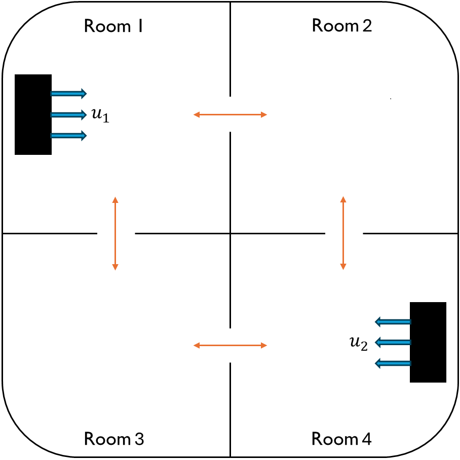
Figure 1: A 4-room thermal system with two inputs

VII-A Single thermal system case

Fig. 1 illustrates the thermal system, with no heat exchange with the environment and two rooms directly connected to the heat conditioner. The model can be represented as $\{\mathcal{V},\mathcal{E}\}$, where $\mathcal{V}$ represents the set of rooms, and $\mathcal{E}$ represents the set of directed heat flow. The red double-sided arrow represents the heat exchange between the adjacent rooms. The heat of this thermal system is depicted by an ordinary differential equation (ODE) with the heat in room $i$ given by

$$\begin{split}\dot{x}_{i}(t)=a_{i}x_{i}(t)+\sum_{(j,i)\in\mathcal{E}}{a_{ij}x_{j}(t)}-\sum_{(i,j)\in\mathcal{E}}{a_{ji}x_{i}(t)}+\\ \sum_{k}{b_{ik}u_{k}(t)}+w_{i}(t)\end{split}$$

where $a_{i}x_{i}(t)$ represents the decay, $a_{ij}x_{j}(t)$ represents the heat flow from room $j$ to room $i$, $a_{ji}x_{i}(t)$ represents the heat flow from room $i$ to room $j$, $b_{ik}u_{k}(t)$ represents the input from actuator $k$ to room $i$, $w_{i}(t)$ is the disturbance. We assume that we can not measure heat continuously due to the digitalization of devices. Therefore, we sample the measurement with interval $\Delta t=0.1s$ and the system can be rewritten as (1) with system matrices listed as follows

$$\begin{split}&A=\left[\begin{matrix}0.5&0.2&0.1&0.0\\ 0.1&0.6&0.0&0.2\\ 0.4&0.0&0.8&0.4\\ 0.0&0.2&0.1&0.4\\ \end{matrix}\right],B=\left[\begin{matrix}0.1&0.0\\ 0.0&0.0\\ 0.0&0.0\\ 0.0&0.1\\ \end{matrix}\right],G=I_{4}\\ &C=\left[\begin{matrix}I_{2}&I_{2}\\ 0_{2}&0_{2}\\ \end{matrix}\right],D=\left[\begin{matrix}0_{2}\\ I_{2}\\ \end{matrix}\right]\end{split}$$

with $C^{T}D=0$, $D^{T}D\succ 0$. The goal is to design an output-feedback controller to minimize the $H_{2}$ norm of the system transfer function, i.e., maximize the system robustness to external disturbance. We run FIPM and SIPM separately to find the solution and compare their performance.

We choose $\epsilon_{1}=1e-5$, $\epsilon_{2}=1e-5$, $\epsilon_{r}=1e-9$, $\delta=1e-9$, $\mu=4$ for FIPM and SIPM. We can easily check $A-I$ is irreducible since $A$ describes a strongly-connected graph. By leveraging Lemma 7 in [10] and take $\mathbf{v}_{1}=\left[\begin{matrix}-4&1\end{matrix}\right]^{T},\mathbf{v}_{2}=\left[\begin{matrix}-2&0\end{matrix}\right]^{T},\mathbf{v}_{3}=\left[\begin{matrix}-1&0\end{matrix}\right]^{T},\mathbf{v}_{4}=\left[\begin{matrix}1&-4\end{matrix}\right]^{T}$, we can initialize $K^{(0)}=\sum_{i}\mathbf{v}_{i}\mathbf{e}_{i}^{T}$ that can make $A-BK$ Schur and compartmental.

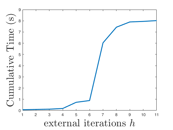
(a) FIPM

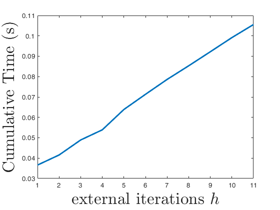
(b) SIPM

Figure 2: Cumulative running time of FIPM and SIPM

Fig. 2(a) shows the cumulative running time of FIPM. After 11 external iterations, the solution converges to

$$K_{F}^{*}=\left[\begin{matrix}0.6334&0.5384&0.6579&0.0000\\ 0.0000&0.5938&0.5182&0.5481\\ \end{matrix}\right]$$

with $J(K_{F}^{*})=26.7744$, which is significantly better than $J(K^{(0)})=128.3285$. Then we check

$$A-BK_{F}^{*}=\left[\begin{matrix}0.4367&0.1462&0.0342&0.0000\\ 0.1000&0.6000&0.0000&0.2000\\ 0.4000&0.0000&0.8000&0.4000\\ 0.0000&0.1406&0.0482&0.3452\\ \end{matrix}\right]$$

which is Schur and compartmental. Now we check if $K_{F}^{*}$ is a stationary point of (8). Denote $t^{(10)}=t^{*}=1048576$. Take

$$\begin{split}&Q^{*}=\cfrac{1}{t^{*}}\cdot\left(\left[\begin{array}[]{c}A_{K}^{*}\\ \mathbf{1}^{T}-\mathbf{1}^{T}A_{K}^{*}\\ \end{array}\right]\right)^{\circ-1}\\ &=\left[\begin{matrix}0.0000&0.0000&0.0000&*\\ 0.0000&0.0000&*&0.0000\\ 0.0000&*&0.0000&0.0000\\ *&0.0000&0.0000&0.0000\\ 0.0000&0.0000&0.0000&0.0000\\ \end{matrix}\right]\geq 0\end{split}$$

where $*$ means do not care since the corresponding entries in $A-BK^{*}_{F}$ are $0$. The KKT conditions hold trivially. However, as shown in Fig. 2(a), it takes 8.0179s to converge, with $||\nabla_{K}JLBF(K_{F}^{*},t^{*})||=3.2739e-04$. In contrast, Fig. 2(b) shows the cumulative running time of SIPM. After 11 external iterations, the solution converges to

$$K_{S}^{*}=\left[\begin{matrix}0.6334&0.5384&0.6579&0.0000\\ 0.0000&0.5938&0.5182&0.5481\\ \end{matrix}\right]$$

with $J(K_{S}^{*})=26.7744$. Hence, FIPM and SIPM finally converge to the same solution. However, it only takes 0.1057s for SIPM to converge, which is about 80 times faster than FIPM. In addition, the gradient of $JLBF$ at the solution $K_{S}^{*}$ is $||\nabla_{K}JLBF(K_{S}^{*},t^{*})||=1.0219e-06$, about 300 times better than FIPM. Therefore, in the case of 4-dimension systems, SIPM shows dominant advantages over FIPM. In the subsequent subsection, we will compare their performance as the system scales increase.

VII-B Multiple thermal systems case

In this subsection, we compare FIPM and SIPM in various system dimensions, specifically in the context of multiple thermal systems. For $N$ thermal systems, we can write the overall system as

$$\begin{split}&A_{N}=\mathrm{blkdiag}(\overbrace{A,\ldots,A}^{N}),B_{N}=\mathrm{blkdiag}(\overbrace{B,\ldots,B}^{N}),G=I_{4},\\ &C_{N}=[\overbrace{C|\ldots|C}^{N}],D_{N}=[\overbrace{D|\ldots|D}^{N}]\end{split}$$

With $K_{N}^{(0)}=\mathrm{blkdiag}(\overbrace{K^{(0)},\ldots,K^{(0)}}^{N})$. The simulation is shown in Table I. The results show that SIPM outperforms FIPM in small-scale systems but is unsuitable for large-scale systems due to the huge computation cost of the Hessian matrix. On the other hand, when $N=10$, $||\nabla_{K}JLBF(K_{F}^{*},t^{*})||=0.0071$ and $||\nabla_{K}JLBF(K_{S}^{*},t^{*})||=7.1495e-12$, FIPM achieves low precision but is faster in large-scale systems.

VIII Conclusion

In this paper, we studied the $H_{2}$ optimal control for compartmental systems. We proposed a novel problem transformation and established an equivalent new optimization problem with closed and polyhedron constraints. We provided FIPM and a novel SIPM to solve the problem, both are guaranteed to converge to a stationary point of the new problem. Meanwhile, we propose an initialization method to guarantee the interior property of initial values. Finally, we conducted thorough simulations to show the pros and cons of FIPM and SIPM.

References

- [1] J. A. Jacquez, Compartmental Analysis in Biology and Medicine: Kinetics of Distribution of Tracer-labeled Materials. Elsevier, 1972.
- [2] W. M. Haddad, V. Chellaboina, and Q. Hui, Nonnegative and Compartmental Dynamical Systems. Princeton University Press, 2010.
- [3] J. A. Jacquez and C. P. Simon, “Qualitative theory of compartmental systems,” SIAM Review, vol. 35, no. 1, pp. 43–79, 1993.
- [4] F.-W. Chang and T. J. Fitzgerald, “Discrete flow modeling: A general discrete time compartmental model,” AIChE Journal, vol. 23, no. 4, pp. 558–567, 1977.
- [5] L. Deng, Z. Shu, and T. Chen, “Event-triggered model predictive control for compartmental systems with application to congestion control of air traffic networks,” in IEEE Conference on Control Technology and Applications (CCTA), 2023, pp. 432–437.
- [6] S. Coogan and M. Arcak, “A compartmental model for traffic networks and its dynamical behavior,” IEEE Transactions on Automatic Control, vol. 60, no. 10, pp. 2698–2703, 2015.
- [7] G. S. Deaecto and J. C. Geromel, “ state feedback control design of continuous-time positive linear systems,” IEEE Transactions on Automatic Control, vol. 62, no. 11, pp. 5844–5849, 2017.
- [8] Y. Ebihara, P. Colaneri, and J. C. Geromel, “ state-feedback control for continuous-time systems under positivity constraint,” in 18th European Control Conference (ECC), 2019, pp. 3797–3802.
- [9] N. Yang, J. Tang, Y. B. Wong, Y. Li, and L. Shi, “Linear quadratic control of positive systems: A projection-based approach,” IEEE Transactions on Automatic Control, vol. 68, no. 4, pp. 2376–2382, 2022.
- [10] M. E. Valcher and I. Zorzan, “State–feedback stabilization of multi-input compartmental systems,” Systems & Control Letters, vol. 119, pp. 81–91, 2018.
- [11] ——, “Continuous-time compartmental switched systems,” in International Symposium on Positive Systems. Springer, 2016, pp. 123–138.
- [12] Z. Yang, N. Yang, and L. Shi, “ controller synthesis for compartmental systems via admm,” IEEE Control Systems Letters, vol. 9, pp. 235–240, 2024.
- [13] P. V. Chanekar, N. Chopra, and S. Azarm, “Optimal structured static output feedback design using generalized benders decomposition,” in 56th IEEE Conference on Decision and Control (CDC), 2017, pp. 4819–4824.
- [14] J.-L. Wu, “Design of optimal static output feedback controllers for linear control systems subject to general structural constraints,” IEEE Transactions on Automatic Control, vol. 67, no. 1, pp. 474–480, 2021.
- [15] ——, “Structured static output feedback mixed / control for linear control systems,” IEEE Transactions on Automatic Control, 2022.
- [16] I. Fatkhullin and B. Polyak, “Optimizing static linear feedback: Gradient method,” SIAM Journal on Control and Optimization, vol. 59, no. 5, pp. 3887–3911, 2021.
- [17] Z. Cheng, J. Ma, X. Li, M. Tomizuka, and T. H. Lee, “Second-order nonconvex optimization for constrained fixed-structure static output feedback controller synthesis,” IEEE Transactions on Automatic Control, vol. 67, no. 9, pp. 4854–4861, 2022.
- [18] G. E. Dullerud and F. Paganini, A Course in Robust Control Theory: A Convex Approach. Springer Science & Business Media, 2013.
- [19] P. L. D. Peres and J. C. Geromel, “ control for discrete-time systems optimality and robustness,” Automatica, vol. 29, no. 1, pp. 225–228, 1993.
- [20] J. Bu, A. Mesbahi, M. Fazel, and M. Mesbahi, “LQR through the lens of first order methods: Discrete-time case,” arXiv preprint arXiv:1907.08921, 2019.
- [21] W. Levine and M. Athans, “On the determination of the optimal constant output feedback gains for linear multivariable systems,” IEEE Transactions on Automatic Control, vol. 15, no. 1, pp. 44–48, 1970.
- [22] J. Nocedal and S. J. Wright, Numerical Optimization. Springer, 1999.
- [23] S. Paternain, A. Mokhtari, and A. Ribeiro, “A newton-based method for nonconvex optimization with fast evasion of saddle points,” SIAM Journal on Optimization, vol. 29, no. 1, pp. 343–368, 2019.
- [24] C. Jin, R. Ge, P. Netrapalli, S. M. Kakade, and M. I. Jordan, “How to escape saddle points efficiently,” in International Conference on Machine Learning. PMLR, 2017, pp. 1724–1732.
- [25] R. Ge, F. Huang, C. Jin, and Y. Yuan, “Escaping from saddle points—online stochastic gradient for tensor decomposition,” in Conference on Learning Theory. PMLR, 2015, pp. 797–842.
- [26] J. J. Liu, N. Yang, K.-W. Kwok, and J. Lam, “Proportional-derivative control of discrete-time positive systems: A state-space approach,” IEEE Transactions on Circuits and Systems II: Express Briefs, 2023.