A gas-surface interaction algorithm for discrete velocity methods in predicting rarefied and multi-scale flows II: For CL boundary model
Abstract
The discrete velocity method (DVM) for rarefied flows and the unified methods (based on the DVM framework) for flows in all regimes have proven to be effective flow solvers over the past decades and have been successfully extended to other important physical fields. Both DVM and unified methods strive to physically model gas-gas interactions. However, for gas-surface interactions (GSI) at the wall boundary, they have only used the full accommodation boundary until now, which deviates from reality. Moreover, the accommodation degrees of momentum and thermal energy are often different. To overcome this limitation and extend the DVM and unified methods to more realistic boundary conditions, an algorithm for the Cercignani-Lampis (CL) boundary with different accommodation degrees of momentum and thermal energy is proposed and integrated into the DVM framework. A Gaussian distribution with slip velocity, including several undetermined parameters, is designed to describe the reflected distribution function. Once the accommodation coefficients (ACs) are known, these undetermined parameters are solved using the relationship between ACs and reflected macroscopic fluxes. In this paper, the Maxwell model and CLL model are adopted as benchmarks to evaluate the performance of the proposed CL model. Additionally, the current CL boundary for the DVM framework considers generality, accommodating both the recently developed efficient unstructured velocity space and the traditional Cartesian velocity space. Moreover, the proposed CL model allows for calculations of both monatomic gases and diatomic gases with internal degrees of freedom. Finally, by being integrated with the unified gas-kinetic scheme within the DVM framework, the performance of the present CL model is validated through a series of benchmark numerical tests across a wide range of Knudsen numbers.
keywords:
Multi-scale flows; Gas-surface interaction; Accommodation coefficient; CL model1 Introduction
Multi-scale flows from earth surface to outer space (or from macroscale to microscale) are common in scenarios such as near-space vehicles and micro-electro-mechanical systems (MEMS), where multiple flow regimes (including continuum, slip, transitional, and free molecular ones) often coexist within a single flow field, leading to complex dynamic process, and challenging the physical modeling and numerical predictions. It is necessary to employ multiple flow models to describe gas-gas interaction (GGI). Additionally, the gas-surface interaction (GSI), which serves as a boundary condition [1], plays an important role in governing aerodynamic forces and heat transfer [2, 3]. As the rarefaction level increases, the impact of the GSI model becomes increasingly significant [4].
In terms of GGI, there are two basic approaches to develop a numerical method for multi-scale flows: domain decomposition strategy and unified strategy [5]. The unified strategy can be further classified into deterministic methods, also referred to as the discrete velocity method (DVM) [6, 7], based on discrete velocity space, as well as stochastic methods based on model particles. Deterministic methods offer significant advantages in simulating low-speed multi-scale flows (without statistical fluctuation). However, they come with the drawback of requiring expensive computational resources when simulating high-speed multi-scale flow [8, 9, 10]. On the other hand, stochastic methods provide notable advantages in simulating high-speed multi-scale flows. Nevertheless, they encounter challenges related to statistical fluctuation when simulating low-speed multi-scale flows. In recent years, a category of unified methods based on discrete velocity has been proposed, such as the unified gas-kinetic scheme (UGKS) [11, 12], discrete unified gas-kinetic scheme (DUGKS) [13, 14], the general synthetic iteration scheme (GSIS) [15, 16], and so on. These advancements make it possible to solve multi-scale flow problems using a unified numerical method. After a decade of development, numerous numerical techniques have been devised and incorporated into these unified methods to enhance computational efficiency and reduce memory costs [17, 18, 19, 20, 21, 22, 23, 24, 25]. With these improvements, unified methods have been successfully applied to a variety of multi-scale flow problems and multi-scale transport problems [26, 27, 28, 29, 30, 31, 32, 33, 34].
In terms of GSI, various GSI models have been developed in the past, such as the Maxwell model [35, 36], the Cercignani–Lampis–Lord (CLL) model [37, 38], and other derivative models [39, 40, 41, 42, 43]. The Maxwell model, combining the diffuse and specular reflection models, is the first and simplest GSI model. It is widely recognized that the Maxwell model only incorporates one accommodation coefficient (AC) [3, 44] and cannot describe the different accommodation degrees of momentum and thermal energy of gas molecules simultaneously [45, 3]. Examples include the normal and tangential momentum AC (NMAC and TMAC), the energy AC (EAC), and the normal and tangential energy AC (NEAC and TEAC). The ACs play a crucial role in aerodynamic and aerothermal predictions and can be calibrated using experimental data [46, 47] or molecular dynamics (MD) simulation results [48, 49, 50, 51]. Cercignani and Lampis proposed a phenomenological GSI model (CL model) that utilizes two independent scattering kernels and ACs for the normal and tangential velocity components of gas molecules (NEAC and TMAC ) [2]. Later, Lord expanded Cercignani and Lampis’s model (known as the CLL model) and implemented it in the direct simulation Monte Carlo (DSMC) method, making it a popular tool for theoretical and computational studies of rarefied gas flows [37, 38]. Taking advantage of the straightforward sampling of reflection velocity, particle methods can seamlessly incorporate the CLL model. Nevertheless, incorporating the GSI model into DVM methods, which necessitate the calculation of the distribution function, poses a challenge. It’s important to note that the CLL model depends on the incident particle velocity, presenting challenges in deriving the corresponding reflection distribution function. In contrast, the scattering kernel of the diffuse model is independent of the incident particle velocity, making it more straightforward to derive the corresponding reflection distribution function. Therefore, in previous research, the DVM has exclusively utilized the fully energy accommodation diffuse model. More recently, Chen et al. introduced a Maxwell boundary algorithm for DVM to predict rarefied and multi-scale flows [52]. In this paper, a new CL model with multi-adjusted accommodation parameters is proposed within the DVM framework. The flow solver is the UGKS with a simplified multi-scale numerical flux [53], accommodating both the recently developed efficient unstructured velocity space [8, 9, 27] and the traditional Cartesian velocity space.
The remainder of the paper is organized as follows: The proposed CL model for DVM is detailed in Sec. 2. In Sec. 3, several numerical simulations, including the supersonic flows over a sharp flat plate, in a microchannel and over a cylinder, are conducted to investigate the performance of the new CL model. Finally, Sec. 4 provides a summary of the work presented in this paper.
2 CL model for the DVM framework
It is well known that the diffuse model follows a Maxwell distribution, characterized by an isotropic Gaussian distribution related to surface temperature. Inspired by this, a simplified anisotropic Gaussian distribution is employed to describe the different accommodation degrees of normal and tangential energy. Consequently, the new model can be viewed as a combination of anisotropic Gaussian reflection and specular reflection. Furthermore, to avoid the complex treatment of the specular model, a tangential reflected velocity is introduced and combined with the simplified anisotropic Gaussian distribution. Consequently, the mathematical expression of the proposed CL model can be stated as follows
| (1) | ||||
where is the reflected distribution function, is the reflected rotational distribution function for diatomic gases [19]. represents the component of the reflected molecular velocity in the local wall coordinate system, where is the normal component pointing toward the flow from the wall, and are the tangential components. and are the wall density and the reflected velocity, respectively. is related to the anisotropic temperature with . , and are the normal temperature, tangential temperature and rotational temperature, respectively. is the gas constant. It should be noted that when , , the present model reverts to the diffuse model
| (2) | ||||
According to literature [45], the distribution function of the diffuse model on the discrete velocity can be decomposed into
| (3) |
where follows a normal distribution
| (4) |
Similarly, the distribution function of Eq. (1) on the discrete velocity can be decomposed into
| (5) |
where
| (6) | ||||
Obviously, the distribution function in Eq. (6) also follows a normal distribution. Furthermore, it is imperative to underscore that, unlike the diffuse model where the three sub-distributions are identical, the present model features distinct sub-distributions. This distinction allows the present model to effectively capture varying degrees of accommodation for both momentum and thermal energy in gas molecules simultaneously.
The expression in Eq. (1) involves six free parameters: , , , , , and , that need to be determined. Once these free parameters are decided, the reflected distribution function, the reflected microscopic flux and the reflected macroscopic flux can be obtained. In this work, the relationship between the ACs and their corresponding reflected macroscopic fluxes is utilized to resolve these parameters. According to Eq. (1), one can calculate the reflected macroscopic flux
| (7) | ||||
where represents the reflected macroscopic flux of . , , , , , , and are the mass flux, normal momentum flux, tangential momentum flux related to , tangential momentum flux related to , total energy flux, normal energy flux, tangential energy flux, and rotational energy flux, respectively.
According to literature [45, 47], the definition of AC is
| (8) |
where and represent the AC and flux of flow variables , and the subscripts , , and denote incidence, reflection and diffuse reflection, respectively. Especially, the mass flux at the wall is zero (i.e., ), resulting in . From Eq. (8), one can obtain
| (9) |
After determining the ACs from either experimental data or MD simulation results, the undetermined free parameters can be resolved by combining Eq. (7) and (9).
As the present CL model is being introduced for the first time, it is crucial to validate its performance. In this study, the results of the Maxwell model and the CLL model will serve as benchmarks to evaluate the proposed model. However, the energy component ACs, NEAC, and TEAC, are also required for the Maxwell model and the CLL model. Therefore, a linear small perturbation CL model is proposed
| (10) | ||||
where a is the new free parameter. It should be noted that the linear small perturbation CL model can only be employed when the following condition is satisfied
| (11) |
Therefore, the free parameters can be obtained
| (12) |
where represents solving the equations group of macroscopic flux G. If the condition 11 is not satisfied, the free parameters for Maxwell model can be calculated as
| (13) | ||||
here, serves as the weight coefficient and is set as the Maxwell AC in this work. For CLL model, the free parameters can be calculated as
| (14) |
3 Numerical experiment
In this section, three test cases are conducted to validate the proposed CL model in the DVM framework. The simulation results from the DS2V software [54] and literature data are used as reference benchmarks.
Generally, four independent characteristic variables are introduced in the non-dimensional reference system, namely, reference length , reference temperature , reference density and reference speed , where is the characteristic length scale of the flow, and are temperature and density of the freestream, respectively. Thus, the following basic non-dimensional quantities can be obtained
| (15) |
One can obtain a complete non-dimensional system by employing these basic quantities. Unless declared otherwise, all variables in the following that lack a “hat” are non-dimensional quantities for simplicity’s sake.
3.1 Supersonic flow over a sharp flat plate
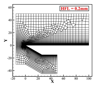
The supersonic flow over a sharp flat plate is simulated to validate the performance of the proposed method in monatomic gas flows. The working gas is argon and the variable hard-sphere (VHS) model with a heat index of is employed. The configuration is the same with the run34 case in Ref. [55]. Figure 1 illustrates the physical space mesh and geometric shape of the sharp flat plate. The height of the first layer (HFL) of the mesh on the surface of the plate is 0.2 . The flat plate has a thickness of 15 and an upper surface length of 100 , forming a sharp angle of 30 degrees. The surface temperature of the flat plate is maintained at 290 K, and the Mach number and temperature of freestream are 4.89 and 116 K, respectively. The Knudsen number of the freestream, with the flat plate’s length as the characteristic length, is 0.0078. Figure 1 illustrates the unstructured velocity space mesh, comprising 896 cells.
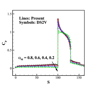
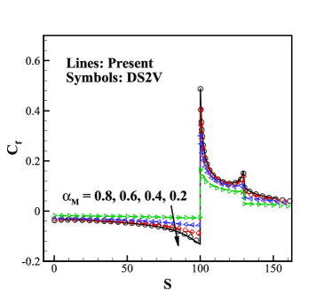
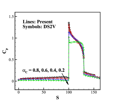
Figure 2 shows the comparison of pressure coefficient, skin friction coefficient and heat transfer coefficient on the surface of flat plate with the Maxwell model. For ease of comparison, the surface coefficients are presented using an S-coordinate system, organized counterclockwise, with the end of the upper surface designated as the origin point. Figure 3 shows the comparison of pressure coefficient, skin friction coefficient and heat transfer coefficient on the surface of flat plate with the CLL model. It can be observed that the results of the present simulation align well with those obtained from DS2V. This demonstrates that the present CL model can be effectively used for flow prediction, serving as either a Maxwell model or a CLL model.
3.2 Supersonic flow in a microchannel
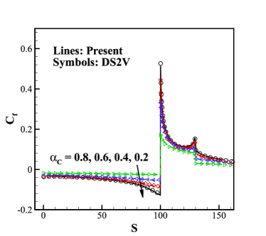
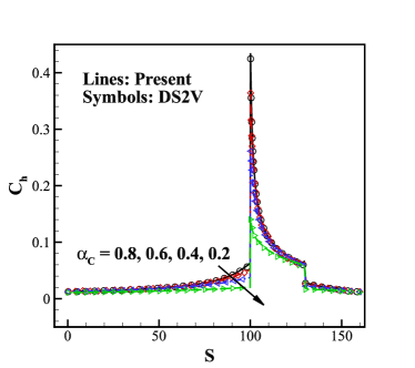
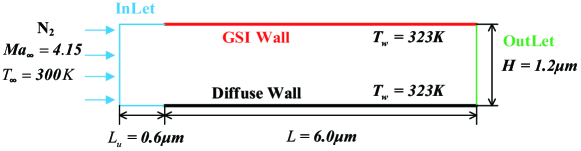
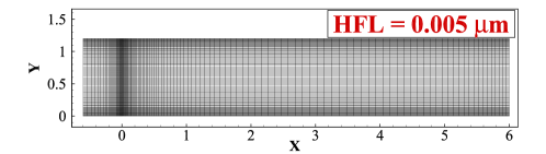
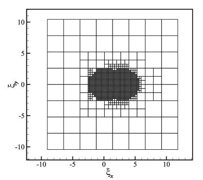
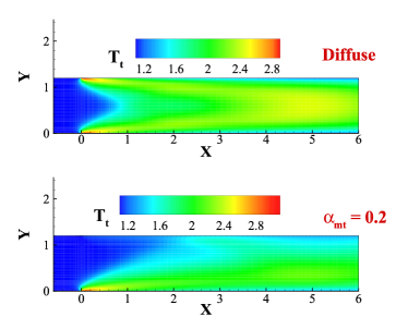
The simulation of supersonic microchannel flow is conducted to validate the performance of the present model in diatomic gas flows. The freestream flow conditions align with those reported in literature [56], and the results from the same literature are utilized as benchmarks. The simulation configuration and computational domain is depicted in Fig. 4. The working gas is nitrogen and the VHS model with is employed. The rotational collision number is 3.5. The Mach number and temperature of freestream are 4.15 and 300 K, respectively. The temperature of the upper and lower surface are both 323 K. The aspect ratio of the microchannel is set at 5, which corresponds to a height of 1.2 and length of 6.0 . Also, the freestream upstream length is 0.6 . In the present study, the characteristic dimension was defined as being the microchannel height . Therefore, the Knudsen number is 0.062. Figure 5 and 6 are the physical space mesh and the velocity space mesh, which have 12348 and 1570 cells.
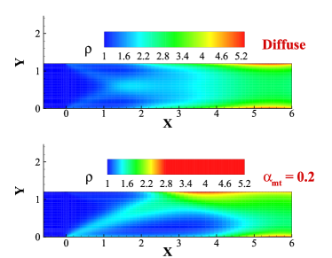
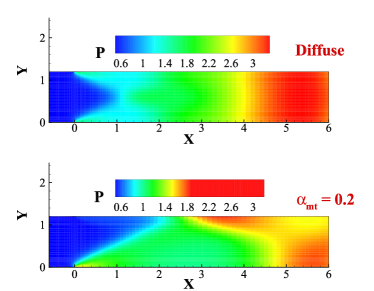
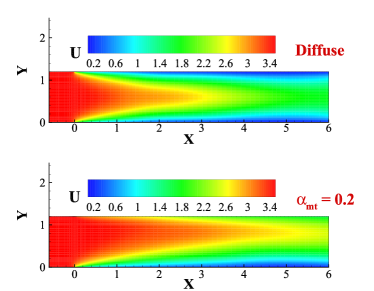
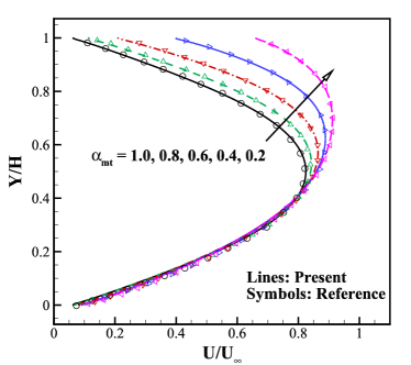
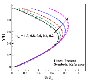
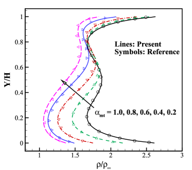
In order to simulate the GSI effects, the diffuse model and the CLL model are employed for the lower and upper wall, respectively. In literature [56], the DSMC method is used to conduct this simulation. Since the flow is parallel to the wall in this case, the NEAC and rotational energy AC are fixed at 1.0 while the TMAC are vary from 1.0 to 0.2. Figure 7 shows the flow contours of density, pressure, horizontal velocity and translational temperature with 1.0 (diffuse model) and 0.2, respectively. The flow structures with are evidently different from those with . Two shock waves are observed at the inlet of the microchannel, resulting in a strong coupling of shock waves and boundary layers inside the microchannel. Moreover, as the TMAC of the upper surface decreases, the upper shock wave becomes weaker. Figure 8 shows the horizontal velocity profiles along the microchannel at X = 2.4 and X = 3.6 with different . As the TMAC decreases, the “retardation” effect of the surface on the tangential flow of the fluid weakens, leading to a gradual increase in the horizontal velocity of the upper surface. Figure 9 depicts the density profiles along the microchannel at X = 2.4 and X = 3.6 with different . Interestingly, the density at the lower surface varies more significantly than the density at the upper surface, once again emphasizing the influence of the coupling of shock waves and boundary layer. Absolutely, it is necessary to emphasize that the present results align well with the references, verifying the effectiveness of the proposed CL model in diatomic gas flow.
3.3 Hypersonic flow over a cylinder
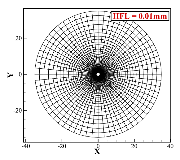
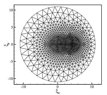
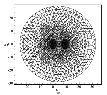
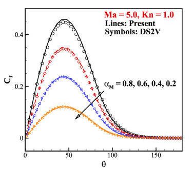
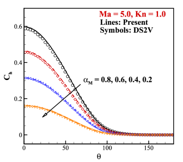
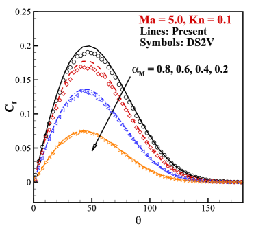
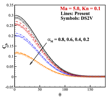
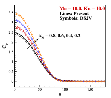
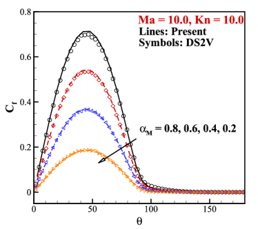
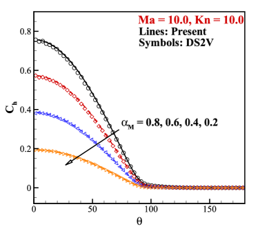
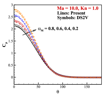
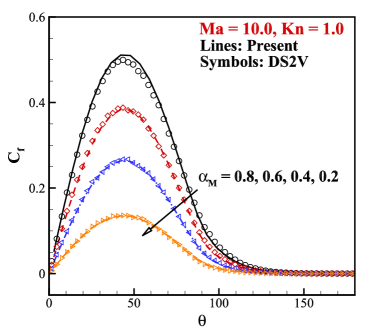
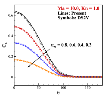
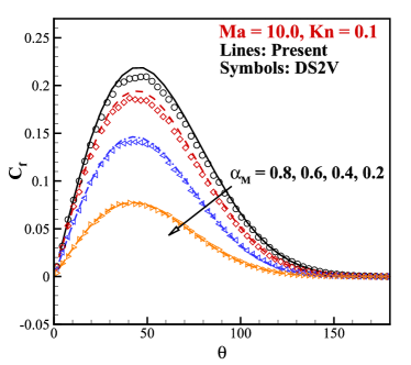
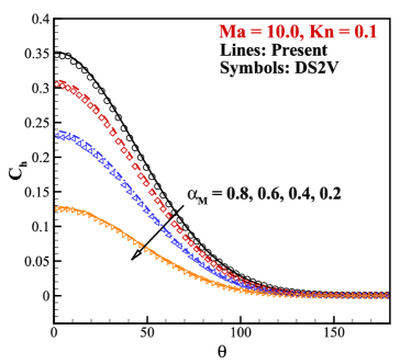
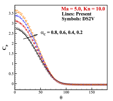
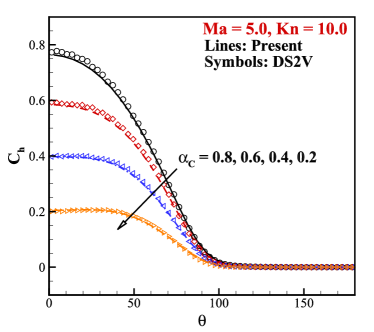
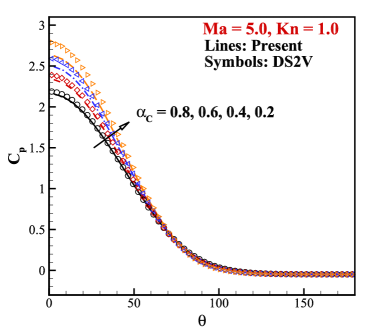
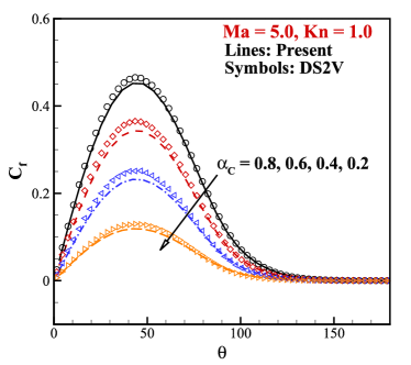
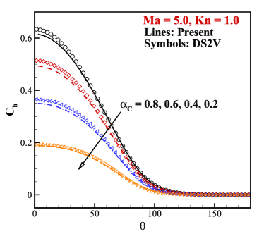
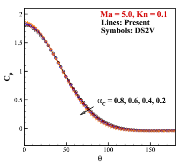
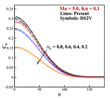
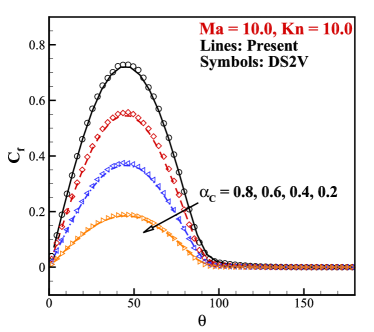
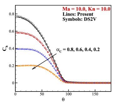
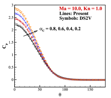
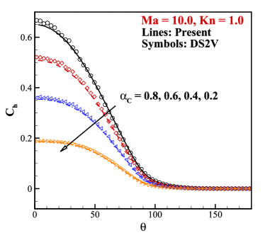
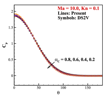
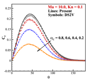
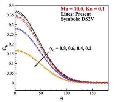
The rarefied hypersonic flow over a cylinder represents a classical multi-scale flow. The performance of the proposed CL model is evaluated across a broad range of Mach numbers and Knudsen numbers. Specifically, two Mach numbers (5.0 and 10.0) and three Knudsen numbers (0.1, 1.0 and 10.0) are considered in the study. Additionally, standard models, including the Maxwell model and CLL model, are employed with ACs ranging from 0.8 to 0.2. The working gas is argon and the VHS model with is utilized. Both the freestream and cylinder surface temperatures are set at 273 K. The cylinder has a radius of 1 , serving as the reference length. Figure 11 illustrates the physical space mesh with a HFL of 0.01 for . Moreover, the HFL for and 0.1 is 0.01 and 0.005 , respectively. Figure 12 presents the unstructured velocity space mesh for (2391 cells) and (2606 cells).
The performance of the proposed CL model in describing the Maxwell-type gas-surface interaction is investigated. In Fig. 13, the pressure coefficient, friction coefficient and heat transfer coefficient of the cylindrical surface are calculated using the Maxwell model with and . The simulation results obtained with the proposed method align closely with those of DS2V under different ACs. Further comparisons of the pressure coefficient, friction coefficient and heat transfer coefficient at the same Mach number are shown in Fig. 14 and Fig. 15, corresponding to Knudsen numbers 1.0 and 0.1, respectively. The simulation results of the present CL model are still very close to the results of DS2V. The comparisons of the pressure coefficient, friction coefficient and heat transfer coefficient at the are shown in Fig. 16, Fig. 17 and Fig. 18, corresponding to 10.0, 1.0 and 0.1, respectively. There is no doubt that the current results agree quite well with the DS2V results. These results underscore the effectiveness of the proposed CL model as an useful Maxwell model. Additionally, the results show that the GSI model have important affect on the aerodynamic force and aerodynamic heat. Certainly, the present results demonstrate a high level of agreement with DS2V, affirming the reliability of the proposed CL model as an effective Maxwell model. Furthermore, the results underscore the noteworthy influence of the GSI model on both aerodynamic force and aerodynamic heat.
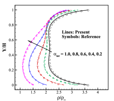
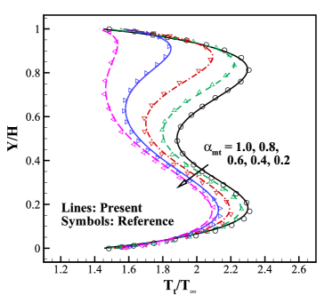
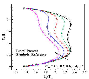
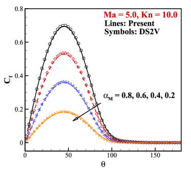
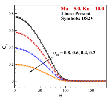
Next, the performance of the proposed CL model in describing the CLL-type gas-surface interaction is also investigated. For simplicity, the TMAC and NEAC are set to the same value, despite their independence and the possibility of having different values. Comparisons of the pressure coefficient, friction coefficient and heat transfer coefficient at are presented in Fig. 19, Fig. 20 and Fig. 21, corresponding to 10.0, 1.0 and 0.1, respectively. Similarly, comparisons at are shown in Fig. 22, Fig. 23 and Fig. 24, corresponding to 10.0, 1.0 and 0.1, respectively. It is evident that the pressure coefficient of the proposed model closely aligns with those of DS2V, except for the peak value with small ACs. More importantly, the proposed model exhibits good agreement with DS2V for friction coefficient and heat transfer coefficient. Overall, the present model can be considered a valid CLL model.
The simulations of hypersonic flow over a cylinder with Mach numbers of 5 and 10 and Knudsen numbers of 10, 1 and 0.1 demonstrate that the proposed CL model can be viewed as either a Maxwell model or a CLL model depending on the selected ACs. The proposed CL model enables DVM methods and unified methods to employ more physical boundary conditions, incorporating different degrees of momentum and energy accommodation, for predicting multi-scale flows.
4 Conclusion
The GSI serves as the source of aerodynamic forces and heat transfer on vehicles, playing a pivotal role in influencing the accuracy of flow predictions. However, the current DVM practice employs only a complete energy accommodation diffuse boundary condition, which is inaccurate for rarefied and multi-scale flows. A novel CL model with different accommodation degrees of momentum and thermal energy is proposed and integrated into the DVM framework. The new CL model obeys an anisotropic Gaussian distribution with reflected velocity and can recover the common Maxwellian distribution, which is an isotropic Gaussian distribution. According to the calculation method of the undetermined parameters of the new CL model, the proposed CL model can be equivalent to the Maxwell model and the CLL model.
The performance of the new CL model is verified by simulating supersonic monatomic gas flow over a sharp flat plate and supersonic diatomic gas flow in a microchannel in the slip regime. Furthermore, the working scope of the CL model is investigated by simulating hypersonic flow over a cylinder across a broad range of Mach numbers and Knudsen numbers. The simulation results prove that the proposed model can effectively describe the interaction of gas and surface in rarefied and multi-scale flow prediction. This makes it possible for DVM and unified methods to employ a more precise boundary condition for predicting the behavior of multi-scale flows and other physical fields.
Acknowledgments
The authors thank Prof. Kun Xu in the Hong Kong University of Science and Technology and Prof. Zhaoli Guo in Huazhong University of Science and Technology for discussions of the UGKS, the DUGKS and multi-scale flow simulations. This work was supported by the National Natural Science Foundation of China (Grant Nos. 12172301 and 12072283) and the 111 Project of China (Grant No. B17037). This work is supported by the high performance computing power and technical support provided by Xi’an Future Artificial Intelligence Computing Center.


References
- [1] F. Sharipov, V. Seleznev, Data on internal rarefied gas flows, Journal of Physical and Chemical Reference Data 27 (3) (1998) 657–706.
- [2] C. Cercignani, M. Lampis, Kinetic models for gas-surface interactions, Transport theory and statistical physics 1 (2) (1971) 101–114.
- [3] M. O. Hedahl, R. G. Wilmoth, Comparisons of the maxwell and cll gas/surface interaction models using dsmc, Tech. rep. (1995).
- [4] W. Santos, M. Lewis, Dsmc calculations of rarefied hypersonic flow over power law leading edges with incomplete surface accommodation, in: 34th AIAA Fluid Dynamics Conference and Exhibit, 2004, p. 2636.
- [5] S. Liu, K. Xu, C. Zhong, Progress of the unified wave-particle methods for non-equilibrium flows from continuum to rarefied regimes, Acta Mechanica Sinica 38 (6) (2022) 122123.
- [6] L. Mieussens, Discrete-velocity models and numerical schemes for the boltzmann-bgk equation in plane and axisymmetric geometries, Journal of Computational Physics 162 (2) (2000) 429–466.
- [7] Z.-H. Li, H.-X. Zhang, Gas-kinetic numerical studies of three-dimensional complex flows on spacecraft re-entry, Journal of Computational Physics 228 (4) (2009) 1116–1138.
- [8] R. Yuan, C. Zhong, A conservative implicit scheme for steady state solutions of diatomic gas flow in all flow regimes, Computer Physics Communications 247 (2020) 106972.
- [9] J. Chen, S. Liu, Y. Wang, C. Zhong, Conserved discrete unified gas-kinetic scheme with unstructured discrete velocity space, Physical Review E 100 (4) (2019) 043305.
- [10] Rui Zhang, Sha Liu, Jianfeng Chen, Congshan Zhuo, Chengwen Zhong, A conservative implicit scheme for three-dimensional steady flows of diatomic gases in all flow regimes using unstructured meshes in the physical and velocity spaces, Physics of Fluids 36 (1) (2024) 016114.
- [11] K. Xu, J.-C. Huang, A unified gas-kinetic scheme for continuum and rarefied flows, Journal of Computational Physics 229 (20) (2010) 7747–7764.
- [12] K. Xu, Direct modeling for computational fluid dynamics: construction and application of unified gas-kinetic schemes, Vol. 4, World Scientific, 2014.
- [13] Z. Guo, K. Xu, R. Wang, Discrete unified gas kinetic scheme for all knudsen number flows: Low-speed isothermal case, Physical Review E 88 (3) (2013) 033305.
- [14] Z. Guo, R. Wang, K. Xu, Discrete unified gas kinetic scheme for all knudsen number flows. ii. thermal compressible case, Physical Review E 91 (3) (2015) 033313.
- [15] W. Su, L. Zhu, P. Wang, Y. Zhang, L. Wu, Can we find steady-state solutions to multiscale rarefied gas flows within dozens of iterations?, Journal of Computational Physics 407 (2020) 109245.
- [16] W. Su, L. Zhu, L. Wu, Fast convergence and asymptotic preserving of the general synthetic iterative scheme, SIAM Journal on Scientific Computing 42 (6) (2020) B1517–B1540.
- [17] S. Chen, K. Xu, C. Lee, Q. Cai, A unified gas kinetic scheme with moving mesh and velocity space adaptation, Journal of Computational Physics 231 (20) (2012) 6643–6664.
- [18] S. Liu, C. Zhong, Modified unified kinetic scheme for all flow regimes, Physical Review E 85 (6) (2012) 066705.
- [19] S. Liu, P. Yu, K. Xu, C. Zhong, Unified gas-kinetic scheme for diatomic molecular simulations in all flow regimes, Journal of Computational Physics 259 (2014) 96–113.
- [20] L. Zhu, Z. Guo, K. Xu, Discrete unified gas kinetic scheme on unstructured meshes, Computers & Fluids 127 (2016) 211–225.
- [21] Y. Wang, C. Zhong, S. Liu, et al., Arbitrary lagrangian-eulerian-type discrete unified gas kinetic scheme for low-speed continuum and rarefied flow simulations with moving boundaries, Physical Review E 100 (6) (2019) 063310.
- [22] S. Chen, C. Zhang, L. Zhu, Z. Guo, A unified implicit scheme for kinetic model equations. part i. memory reduction technique, Science bulletin 62 (2) (2017) 119–129.
- [23] Y. Zhu, C. Zhong, K. Xu, Implicit unified gas-kinetic scheme for steady state solutions in all flow regimes, Journal of Computational Physics 315 (2016) 16–38.
- [24] Q. Zhang, Y. Wang, D. Pan, J. Chen, S. Liu, C. Zhuo, C. Zhong, Unified x-space parallelization algorithm for conserved discrete unified gas kinetic scheme, Computer Physics Communications 278 (2022) 108410.
- [25] M. Zhong, S. Zou, D. Pan, C. Zhuo, C. Zhong, A simplified discrete unified gas kinetic scheme for incompressible flow, Physics of Fluids 32 (9) (2020) 093601.
- [26] L. Zhu, Z. Guo, Numerical study of nonequilibrium gas flow in a microchannel with a ratchet surface, Physical Review E 95 (2) (2017) 023113.
- [27] J. Chen, S. Liu, Y. Wang, C. Zhong, A compressible conserved discrete unified gas-kinetic scheme with unstructured discrete velocity space for multi-scale jet flow expanding into vacuum environment, Commun. Comput. Phys 28 (2020) 1502–1535.
- [28] Guang Zhao, Chengwen Zhong, Sha Liu, Jianfeng Chen, Congshan Zhuo, Numerical simulation of lateral jet interaction with rarefied hypersonic flow over a two-dimensional blunt body, Physics of Fluids 35 (8) (2023) 086107.
- [29] R. Zhang, C. Zhong, S. Liu, C. Zhuo, Large-eddy simulation of wall-bounded turbulent flow with high-order discrete unified gas-kinetic scheme, Advances in Aerodynamics 2 (1) (2020) 1–27.
- [30] Z. Yang, C. Zhong, C. Zhuo, et al., Phase-field method based on discrete unified gas-kinetic scheme for large-density-ratio two-phase flows, Physical Review E 99 (4) (2019) 043302.
- [31] W. Sun, S. Jiang, K. Xu, An asymptotic preserving unified gas kinetic scheme for gray radiative transfer equations, Journal of Computational Physics 285 (2015) 265–279.
- [32] Z. Guo, K. Xu, Discrete unified gas kinetic scheme for multiscale heat transfer based on the phonon boltzmann transport equation, International Journal of Heat and Mass Transfer 102 (2016) 944–958.
- [33] D. Pan, C. Zhong, C. Zhuo, W. Tan, A unified gas kinetic scheme for transport and collision effects in plasma, Applied Sciences 8 (5) (2018) 746.
- [34] T. Shuang, S. Wenjun, W. Junxia, N. Guoxi, A parallel unified gas kinetic scheme for three-dimensional multi-group neutron transport, Journal of Computational Physics 391 (2019) 37–58.
- [35] E. H. Kennard, et al., Kinetic theory of gases, Vol. 483, McGraw-hill New York, 1938.
- [36] J. C. Maxwell, Vii. on stresses in rarified gases arising from inequalities of temperature, Philosophical Transactions of the royal society of London (170) (1879) 231–256.
- [37] R. Lord, Some extensions to the cercignani–lampis gas–surface scattering kernel, Physics of Fluids A: Fluid Dynamics 3 (4) (1991) 706–710.
- [38] R. Lord, Some further extensions of the cercignani–lampis gas–surface interaction model, Physics of Fluids 7 (5) (1995) 1159–1161.
- [39] H. Struchtrup, Maxwell boundary condition and velocity dependent accommodation coefficient, Physics of Fluids 25 (11) (2013).
- [40] S. Brull, P. Charrier, L. Mieussens, Nanoscale roughness effect on maxwell-like boundary conditions for the boltzmann equation, Physics of Fluids 28 (8) (2016).
- [41] L. Wu, H. Struchtrup, Assessment and development of the gas kinetic boundary condition for the boltzmann equation, Journal of Fluid Mechanics 823 (2017) 511–537.
- [42] K. Yamamoto, H. Takeuchi, T. Hyakutake, Scattering properties and scattering kernel based on the molecular dynamics analysis of gas-wall interaction, Physics of Fluids 19 (8) (2007).
- [43] M. Hossein Gorji, P. Jenny, A gas-surface interaction kernel for diatomic rarefied gas flows based on the cercignani-lampis-lord model, Physics of fluids 26 (12) (2014).
- [44] S. A. Peddakotla, K. K. Kammara, R. Kumar, Molecular dynamics simulation of particle trajectory for the evaluation of surface accommodation coefficients, Microfluidics and Nanofluidics 23 (2019) 1–17.
- [45] Q. Shen, Rarefied gas dynamics, National Defense Industry Press, 2003.
- [46] I. Kinefuchi, Y. Kotsubo, K. Osuka, Y. Yoshimoto, N. Miyoshi, S. Takagi, Y. Matsumoto, Incident energy dependence of the scattering dynamics of water molecules on silicon and graphite surfaces: the effect on tangential momentum accommodation, Microfluidics and Nanofluidics 21 (2017) 1–13.
- [47] W. Liu, J. Zhang, Y. Jiang, L. Chen, C.-H. Lee, Dsmc study of hypersonic rarefied flow using the cercignani–lampis–lord model and a molecular-dynamics-based scattering database, Physics of Fluids 33 (7) (2021).
- [48] V. Chirita, B. Pailthorpe, R. Collins, Non-equilibrium energy and momentum accommodation coefficients of ar atoms scattered from ni (001) in the thermal regime: A molecular dynamics study, Nuclear Instruments and Methods in Physics Research Section B: Beam Interactions with Materials and Atoms 129 (4) (1997) 465–473.
- [49] J. Reinhold, T. Veltzke, B. Wells, J. Schneider, F. Meierhofer, L. C. Ciacchi, A. Chaffee, J. Thöming, Molecular dynamics simulations on scattering of single ar, n2, and co2 molecules on realistic surfaces, Computers & Fluids 97 (2014) 31–39.
- [50] W. W. Lim, G. J. Suaning, D. R. McKenzie, A simulation of gas flow: The dependence of the tangential momentum accommodation coefficient on molecular mass, Physics of Fluids 28 (9) (2016).
- [51] N. Andric, P. Jenny, Molecular dynamics investigation of energy transfer during gas-surface collisions, Physics of Fluids 30 (7) (2018).
- [52] J. Chen, S. Liu, C. Zhong, Y. Wang, C. Zhuo, Y. Yang, A gas-surface interaction algorithm for discrete velocity methods in predicting rarefied and multi-scale flows, Available at SSRN 4236130.
- [53] R. Zhang, S. Liu, C. Zhong, C. Zhuo, Unified gas-kinetic scheme with simplified multi-scale numerical flux for thermodynamic non-equilibrium flow in all flow regimes, Communications in Nonlinear Science and Numerical Simulation 119 (2023) 107079.
- [54] G. A. Bird, Molecular gas dynamics and the direct simulation of gas flows, Oxford university press, 1994.
- [55] N. Tsuboi, Y. Matsumoto, Experimental and numerical study of hypersonic rarefied gas flow over flat plates, AIAA journal 43 (6) (2005) 1243–1255.
- [56] I. B. Sebastião, W. F. Santos, Gas–surface interaction effects on the flowfield structure of a high speed microchannel flow, Applied thermal engineering 52 (2) (2013) 566–575.