Connecting the hexagonal closed packed structure with the cuboidal lattices: A Burgers-Bain type martensitic transformation for a Lennard-Jones solid derived from exact lattice summations

Abstract

The diffusionless martensitic phase transition from a hexagonal close-packed (hcp) arrangement to the face-centered close-packed (fcc) and subsequently the body-centered cubic (bcc) lattice is discussed for a Lennard-Jones solid. The associated generalized lattice vectors to construct the underlying bi-lattice for a Burgers-Bain-type of transformation require a minimum of a four-parameter space $(a,\alpha,\beta,\gamma=c/a)$, describing, beside the change in the base lattice parameters $a$ and $c$ of a hexagonal or cuboidal cell, the shear force acting on the hexagonal base plane through the parameter $\alpha$, and the sliding force of the middle layer in the original AB hexagonal packing arrangement through the parameter $\beta$. The Bain part of the transformation depends only on two parameters $a$ and $\gamma$, describing a cuboidal transition within a body-centered tetragonal cell. By optimizing the lattice parameters $a$ and $\beta$ for a $(n,m)$-Lennard-Jones potential, we obtain a simple two-dimensional picture for the complete Burgers-Bain-type hcp$\leftrightarrow$fcc$\leftrightarrow$bcc phase transition. From the generalized lattice vectors we were able to construct the corresponding lattice sums in terms of inverse power potentials applying fast converging Bessel function expansions using a Terras decomposition of the Epstein zeta function combined with a Van der Hoff-Benson expansion for the lattice sums. This allows the cohesive energy to be determined to computer precision for a Lennard-Jones solid. For six different combinations of $(n,m)$-Lennard-Jones potentials the energy $(\alpha,\gamma)$ hypersurface was then mapped out and studied in more detail. There has been a long controversy if the fcc phase is required for the hcp$\leftrightarrow$bcc phase transition (two-step model). We show that for a Lennard-Jones model the minimum energy path is found to be indeed a two-step hcp$\rightarrow$fcc$\rightarrow$bcc transition process. The lowest transition state in each case can be regarded as an upper limit to a hypothetical true minimum energy path out of the many possibilities in a hcp$\leftrightarrow$fcc$\leftrightarrow$bcc phase transition.

I Introduction

The relative stability between the face-centred cubic (fcc) and hexagonal close-packed (hcp) structures, and their formation from the gas or the liquid phase known as the nucleation problem, has been a matter of intense discussion and debate over the past 50 years.Sanchez-Burgos et al. (2021) Both phases have the same hard-sphere packing density of $\rho=\pi/3\sqrt{2}$=0.74048048969…, as have all possible associated Barlow structures (mixtures between (AB)_∞ and (ABC)_∞ stackings)Barlow (1883); Osang, Edelsbrunner, and Saadatfar (2021) for which there are infinitely many. It was only in recent times that Kepler’s original conjecture, stating that the fcc packing density cannot be surpassed for hard (unit) sphere packings and therefore is optimal, was proven by Hales.Hales (2011, 2005)

Optimal sphere packings predict only a very small difference in the free energy up to the melting point.Frenkel and Ladd (1984); Woodcock (1997); Sanchez-Burgos et al. (2021) For real atomic or molecular crystals the two close-packed structures are also found to be very close in energy.Krainyukova (2011) A prominent example is solid argon, where at low temperatures and pressures, vibrational effects need to be included to stabilize the experimentally observed fcc over the hcp phase,Moyano, Schwerdtfeger, and Rosciszewski (2007); Schwerdtfeger et al. (2016). However, the cohesive energy difference between the two phases is predicted to be a mere 8.8 J/mol at zero temperature and pressure.Schwerdtfeger et al. (2016) Such small energy differences between the fcc and hcp phase for solids are also detected in nucleation processes Senger et al. (1999); Lovett (2007); Lu and Li (1998); Schwerdtfeger et al. (2006). On the other hand, for the heavier noble gas elements the hcp phase becomes the dominant phase at high pressures,Cynn et al. (2001); Rosa et al. (2018); Dewaele et al. (2021) which is most likely due to the fact that with increasing pressure vibrational effects become less important compared to the competing many-body electronic contributions.

Why one phase dominates over the other at certain temperatures and pressures delicately depends on the different static and dynamic contributions to the free energy. It is however notoriously difficult to get a detailed mechanistic insight into such solid-state phase transitions by both experimental and theoretical methods,Caspersen and Carter (2005) and therefore such transitions are in general not well understood.Stillinger (2001); Jackson, Bruce, and Ackland (2002) One could naively slide some of the hexagonal layers to turn hcp into fcc, i.e. for the hexagonal layer sequences we have the transformation (ABA$\downarrow$B$\downarrow$A$\uparrow$B$\uparrow$)${}_{\infty}\rightarrow$(ABCABC)_∞.Jackson, Bruce, and Ackland (2002) However, it is not known if this is the optimal minimum energy path, for example, in such sliding of the hexagonal layers one may well access local minima such as dense Barlow packings, e.g. (ABABA$\downarrow$B)${}_{\infty}\rightarrow$(ABABCB)_∞.

In 1934 Burgers suggested a very simple diffusionless hcp$\leftrightarrow$bcc phase transition pathBurgers (1934), while Bain earlier in 1924 proposed a simple cuboidal fcc$\leftrightarrow$bcc transition path Bain (1924). Since then, there has been some controversy whether or not the fcc phase is actually required in a minimum energy path for the hcp$\rightarrow$bcc phase transition and if these transitions follow at all the diffusionless mechanism as suggested by Bain and Burgers.Cayron (2013); Lu et al. (2014); Cayron (2015, 2016)

Modeling solid-state phase transitions at the microscopic level poses significant challenges.Raghavan and Cohen (1975); Gooding and Krumhansl (1988); Caspersen and Carter (2005); Johnson and Carter (2008); Torrents et al. (2017); Li, Qian, and Li (2021) This is mainly due to the fact that often stacking faults or defects are involved in such phase changes, which requires a computationally expensive super-cell treatment in a molecular dynamics simulation.Bruinsma and Zangwill (1985); Dovesi and Orlando (1994); Li et al. (2017) Moreover, various theoretical approximations (such as the density functional approximation) may not result in the correct energy sequence between the different polymorphs involved.Liu et al. (2003) Diffusionless martensitic transformations do not have these problems, but mapping out the correct minimum energy path for such a transition can be a formidable task.Rifkin (1984); Sandoval, Urbassek, and Entel (2009); Cayron (2013, 2015); Li et al. (2017)

Caspersen and Carter Caspersen and Carter (2005) generalized the climbing image-nudged elastic band algorithm to find transition paths in solid-state phase transitions, and subsequently applied this to the diffusionless martensitic transformation Bain (1924); Burgers (1934) from hcp to the body-centered cubic (bcc) structure and further to fcc for metallic lithium. They gave detailed information for the transformation matrices acting on the corresponding lattice vectors. In a different approach, Raju Natarajan and Van der Ven used a set of two parameters derived from the Hencky logarithmic strain to map out the volume preserving potential energy surfaces for the Burgers-Bain transformation for metallic lithium, sodium and magnesium.Raju Natarajan and Van der Ven (2019) Cayron introduced transformation matrices (which he termed angular distortive matrices) for continuous atomic displacements between the three different phases.Cayron (2016) Bingxi Li et al. performed molecular dynamics simulations using a (12,6)-Lennard-Jones potential for argon calibrated at $T=40$ K and $P=1$ bar.Li et al. (2017) They discussed different paths for the hcp$\leftrightarrow$fcc phase transition. However, the topology of the cohesive energy dependent of the lattice parameters sensitive to such phase transition may critically depend on the chosen model describing the interactions between the atoms in the lattice. Moreover, molecular dynamics (MD) or Monte-Carlo simulations for the phase transitions in the solid state are computer time consuming and depend on the size of the supercell chosen. Hence, it would be advantageous to develop a simpler model capable of estimating the activation energy involved in such solid-state phase transitions.

In this paper we analyze in detail the Burgers-Bain hexagonal-to-cuboidal transformation path from hcp$\rightarrow$fcc$\rightarrow$bcc for the case of a general $(n,m)$ Lennard-Jones (LJ) potential ($n>m,m>3$),Jones (1924); Jones and Ingham (1925)

$$V_{\textrm{LJ}}(r)=\frac{\epsilon nm}{n-m}\;\left[\frac{1}{n}\left(\frac{r_{e}}{r}\right)^{n}-\frac{1}{m}\left(\frac{r_{e}}{r}\right)^{m}\right]$$ (1)

describing the interactions between the atoms in a solid using exact lattice summations to obtain the cohesive energy.Borwein et al. (2013); Burrows et al. (2020); Schwerdtfeger, Burrows, and Smits (2021) Here, $\epsilon$ and $r_{e}$ are the binding energy and the equilibrium distance of the diatomic molecule, respectively. Both of these parameters can be arbitrarily set to 1 in order to express them in dimensionless units. For very large exponents $n,m$ the LJ potential approaches the kissing hard-sphere (KHS) model with $V(r)=\infty$ for $r<r_{e}$, $V(r)=-\epsilon$ for $r=r_{e}$, and $V(r)=0$ for $r>r_{e}$ as originally introduced by Baxter Baxter (1968); Stell (1991).

We have recently shown that the Bain transformation can be effectively described within a two-parameter space $(A,r_{\text{NN}})$,Jerabek, Burrows, and Schwerdtfeger (2022) where $r_{\text{NN}}$ is the nearest neighbor distance in the solid and $A$ is responsible for describing the martensitic transformation path from the axial centred-cuboidal (acc) lattice ($A=1/3$), to the bcc lattice ($A=1/2$), the mean centred-cuboidal (mcc) lattice ($A=1/\sqrt{2}$), and finally the face-centred cubic (fcc) lattice ($A=1$) in a general body-centered tetragonal (bct) arrangement. The advantage of this choice of parameters instead of the usual bct lattice parameters $(a,c)$ is that the nearest neighbor distance changes only slightly along the Bain transformation path and a two-dimensional picture can therefore be avoided. We will show that a similar choice of parameters can be used to describe the Burgers transformation from hcp to fcc, and demonstrate that a very simple transformation emerges to describe the Burgers-Bain transformation. The formalism can be used for future density functional studies and the activation energy obtained can be seen as an upper bound to the true (and possibly more complex) minimum energy path.

In the coming section we present the theory of the Burgers-Bain hcp$\leftrightarrow$fcc$\leftrightarrow$bcc transformation and develop the corresponding lattice sums for inverse power potentials. We then apply these lattice sums to various $(n,m)$ Lennard-Jones potentials and discuss the results for the transition paths. We will show that for such potentials, starting from hcp phase, the minimum energy transition path leads to fcc rather than directly to the bcc phase within the parameter space chosen. A conclusion and future perspectives on this topic is given in the final section.

II Theory

In order to discuss the martensitic phase transition along a Burgers- or Bain-type path,Bain (1924); Burgers (1934) we need to introduce the various lattices parameters involved and discuss their transformation properties, matrices and corresponding lattice sums for inverse power potentials.

II.1 Lattice vectors and properties

II.1.1 The hexagonal close packed structure

The hcp phase is a bi-lattice Middlemas, Stillinger, and Torquato (2019) that requires two hexagonal Bravais lattices to describe the close-packed structure, or alternatively one hexagonal unit cell with one atom positioned inside specified by its Wyckoff position (fractional Cartesian coordinates) $(0,0,0)$ and $(\frac{1}{3},\frac{2}{3},\frac{1}{2})$. It belongs together with the fcc lattice to the more general class of densest packed Barlow multi-lattices Barlow (1883).

To correctly describe the Burgers-Bain martensitic hcp$\leftrightarrow$fcc$\leftrightarrow$bcc phase transition we describe the cuboidal lattice within the smallest common unit cell, that is a hexagonal-like cell with two specified layers A and B as shown in Figure 1. We then introduce a common set of basis vectors containing parameters that transform the lattices smoothly into each other.

Figure 1: The (distorted) cuboidal (blue lines shown on the left) and the hcp structure both with a ABABAB… sequence (layers A in red and B in blue) shown in a hexagonal unit cell with corresponding basis vectors with cell parameters $|\vec{b}_{1}|=|\vec{b}_{2}|=a$, and $|\vec{b}_{3}|=c$. The ratio $\gamma=c/a=\sqrt{8/3}$ together with $\angle(\vec{b}_{1},\vec{b}_{2})=60^{\circ}$ leads to the optimal hcp lattice with 12 kissing spheres around a central atom. For $c=a$ and and $\angle(\vec{b}_{1},\vec{b}_{2})=90^{\circ}$ to we obtain the bcc lattice with 8 kissing spheres. Alternatively, we have $c/a=\sqrt{2}$ and $\angle(\vec{b}_{1},\vec{b}_{2})=90^{\circ}$ for the fcc lattice with 12 kissing spheres.

For the hexagonal-to-cuboidal hcp$\rightarrow$cub (cub $=$ fcc or bcc for example) Burgers phase transition we start by considering the underlying hexagonal Bravais lattice (h) with the accompanying basis vectors,

$$\vec{b}_{1}^{\top}=a\left(1,0,0\right),\quad\vec{b}_{2}^{\top}=a\left(\frac{1}{2},\frac{\sqrt{3}}{2},0\right),\quad\vec{b}_{3}^{\top}=c\left(0,0,1\right)\,.$$ (2)

with the lattice parameters $|\vec{b}_{1}|=|\vec{b}_{2}|=a$ and $|\vec{b}_{3}|=c$, and $\angle(\vec{b}_{1},\vec{b}_{2})=60^{\circ}$ and $\angle(\vec{b}_{1},\vec{b}_{3})=\angle(\vec{b}_{2},\vec{b}_{3})=90^{\circ}$. We define the generator matrix consisting of these three vectors as

$$B_{h}=\begin{pmatrix}\vec{b}_{1}^{\top}\\ \vec{b}_{2}^{\top}\\ \vec{b}_{3}^{\top}\end{pmatrix}=a\begin{pmatrix}1&0&0\\ \frac{1}{2}&\frac{\sqrt{3}}{2}&0\\ 0&0&\gamma\end{pmatrix}$$ (3)

where we use the notation $\gamma=\frac{c}{a}$. This leads to the following positive definite symmetric Gram matrix

$$\left(G_{ij}\right)_{h}=\left(\vec{b}_{i}^{\top}\vec{b}_{j}\right)=a^{2}\begin{pmatrix}1&\frac{1}{2}&0\\ \frac{1}{2}&1&0\\ 0&0&\gamma^{2}\end{pmatrix}$$ (4)

with det$(G)=\frac{3}{4}a^{4}c^{2}=\frac{3}{4}a^{6}\gamma^{2}>0$. From an arbitrarily chosen atom at the origin, all points in the hexagonal lattice (A layers only) are described by

$$\vec{r}^{h}_{1}(\vec{i})=B_{h}^{\top}\vec{i}=i_{1}\vec{b}_{1}+i_{2}\vec{b}_{2}+i_{3}\vec{b}_{3}\\$$ (5)

with $\vec{i}\in\mathbb{Z}^{3}$. Their distances to the origin are given by the quadratic form

$$|\vec{r}^{h}_{1}(\vec{i})|=\left(\vec{i}^{\top}G_{h}\vec{i}\right)^{\frac{1}{2}}=a\left(i_{1}^{2}+i_{1}i_{2}+i_{2}^{2}+\gamma^{2}i_{3}^{2}\right)^{\frac{1}{2}}\,.$$ (6)

The volume of the unit cell is determined through the Gram matrix

$$V(a,\gamma)=\sqrt{{\textrm{det}}G}=\frac{\sqrt{3}}{2}a^{3}\gamma$$ (7)

The nearest neighbor distance is given by

$$r^{h}_{\textrm{NN}}(a,c)=\textrm{min}\{r^{h}_{1}(\vec{i})\}={\textrm{min}}\left\{a,c\right\}\,.$$ (8)

and the kissing number for a lattice $\mathscr{L}$ is defined as

$$\kappa(\mathscr{L})=\#\{\vec{r}(\vec{i})\in\mathscr{L}~{}|~{}|\vec{r}(\vec{i})|=r_{\text{NN}}(\mathscr{L})\}$$ (9)

For the hcp structure with ideal value of $\gamma_{\textrm{hcp}}=\sqrt{\tfrac{8}{3}}$ the kissing number is $\kappa=12$. Similarly, we have $\kappa=12$ for fcc and $\kappa=8$ for bcc.

We now introduce the second layer, i.e. the B-layer as shown in Figure 1, to complete the hcp structure. The B-layer is shifted by a vector of $\vec{v}_{h}^{\top}=\frac{a}{2}\left(1,\frac{1}{\sqrt{3}},\gamma\right)$ with respect to the lattice vectors given in (2), such that the position of any atom in the B layers is given by

$$\vec{r}^{h}_{2}(\vec{i}) =B_{h}^{\top}\vec{i}+\vec{v}_{h}\;,$$ (10)

The shift vector can easily be derived from the fact that an atom in the B layer sits above the centroid of a triangle of neighboring lattice points in the A layer. We call the set $\{\vec{b}_{i},\vec{v}_{h}\}$ generalized lattice vectors. They include the Wyckoff positions within a unit cell. The resulting set of distance vectors $\{\vec{r}^{h}_{1}(\vec{i}),\vec{r}^{h}_{2}(\vec{i})\}$ then produce all points in 3D space for the hcp bi-lattice. For the minimum distance $r^{h}_{\textrm{NN}}$ in an hcp bi-lattice we now have,

$$r^{h}_{\textrm{NN}}(a,\gamma)={\textrm{min}}\left\{a,c,\sqrt{\frac{a^{2}}{3}+\frac{c^{2}}{4}}\right\}=a\,{\textrm{min}}\left\{1,\gamma,\sqrt{\frac{1}{3}+\frac{1}{4}\gamma^{2}}\right\}\,.$$ (11)

II.1.2 Connecting the body-centered cuboidal with the hexagonal structure

From Figure 1 we see how the hcp and bcc structures are related to each other and can easily be smoothly transformed into each other which is what Burgers had in mind in his original 1934 paperBurgers (1934). We therefore start with the cuboidal phase described within a hexagonal lattice. The basis vectors for the simple cubic (c) unit cell are,

$$\vec{b^{\prime}}_{1}^{\top}=a\left(1,0,0\right),\quad\vec{b^{\prime}}_{2}^{\top}=a\left(0,1,0\right),\quad\vec{b^{\prime}}_{3}^{\top}=a\left(0,0,\gamma\right)\,.$$ (12)

with $|\vec{b}^{\prime}_{1}|=|\vec{b}^{\prime}_{2}|=|\vec{b}^{\prime}_{3}|=a$, and $\angle(\vec{b}_{1},\vec{b}_{2})=\angle(\vec{b}_{1},\vec{b}_{3})=\angle(\vec{b}_{2},\vec{b}_{3})=90^{\circ}$. We conveniently keep $\gamma$ in the definition of the generator matrix for the bcc lattice as it becomes important later for the definition of the fcc lattice,

$$B_{c}=a\begin{pmatrix}1&0&0\\ 0&1&0\\ 0&0&\gamma\end{pmatrix}$$ (13)

For $\gamma=1$ we obtain the generator matrix of a simple cubic lattice. We can already see the familiarity between the two matrices $B_{h}$ and $B_{c}$. This gives the following Gram matrix,

$$G_{c}=a^{2}\begin{pmatrix}1&0&0\\ 0&1&0\\ 0&0&\gamma^{2}\end{pmatrix}$$ (14)

with det$(G)=a^{6}\gamma^{2}$ which gives det$(G)=1$ for $a=\gamma=1$. The volume is therefore $V(a,\gamma)=a^{3}\gamma$ or for the ideal bcc lattice $V=a^{3}$. The distances are given by (A layers only) $\vec{r}^{c}_{1}(\vec{i})=B_{c}^{\top}\vec{i}$, and we have the expression in terms of the quadratic form $(\vec{i}^{\top}G_{c}\vec{i})$,

$$|\vec{r}^{c}_{1}(\vec{i})|=\left(\vec{i}^{\top}G_{c}\vec{i}\right)^{\frac{1}{2}}=a\left(i_{1}^{2}+i_{2}^{2}+\gamma^{2}i_{3}^{2}\right)^{\frac{1}{2}}\,.$$ (15)

We now address again the B-layer in Figure 1 for the bcc lattice by using the shift vector $\vec{v}_{c}^{\top}=\frac{a}{2}\left(1,1,\gamma\right)$ with length $\vec{v}_{c}=\frac{a}{2}\sqrt{2+\gamma^{2}}$. The distances are given by $\vec{r}^{c}_{2}(\vec{i})=B_{c}^{\top}\vec{i}+\vec{v}_{c}$. Again, the set of both vectors $\{\vec{r}^{c}_{1}(\vec{i}),\vec{r}^{c}_{2}(\vec{i})\}$ produce all points in 3D space for the bcc lattice. So far we have a two-parameter space for the distances $\vec{r_{k}}(a,\gamma)$ for the two lattices hcp and bcc. They will become variable parameters when we discuss the Lennard-Jones potential further below.

There is one important fact to note. In the anticipated hcp$\leftrightarrow$bcc transformation we start with an hcp multi-lattice using the hexagonal primitive cell as the underlying unit cell which transforms along the Bain path into a simple cubic multi-lattice. This cubic unit cell is not the primitive bcc cell. In fact, the smallest distance in the bcc cell is given along the [111] direction to the center lattice point with a distance of $a_{c}=|\vec{v}_{c}|=a\sqrt{3}/2$ for $\gamma=1$. Lennard-Jones and Ingham therefore introduced an additional multiplicative factor to the lattice for the bcc cell Jones and Ingham (1925), which we discuss further below for the more general Burgers transformation between the hcp and the cuboidal lattices.

II.1.3 The Burgers-Bain transformation

We derive the Burgers transformation between the two lattices hcp and bcc in a similar way to the Bain transformation in Ref. Burrows, Cooper, and Schwerdtfeger, 2021a. We first note that

$$B_{h}=U_{B}B_{c}=\begin{pmatrix}1&0&0\\ \frac{1}{2}&\frac{\sqrt{3}}{2}&0\\ 0&0&1\end{pmatrix}B_{c}$$ (16)

This means that the distances transform like $\vec{r}_{k}^{h}=U_{B}\vec{r}_{k}^{c}~{}(k=1,2)$. For the second set of distances we therefore have to consider the transformation of the shift vector as well

$$\vec{v^{\prime}}=U_{B}\vec{v}^{c}_{c}=\frac{a}{2}\left(1,\tfrac{1}{2}(1+\sqrt{3}),\gamma\right)^{\top}$$ (17)

The vector $\vec{v^{\prime}}$ differs markedly from $\vec{v}^{h}$ only in its second component. It is therefore necessary to introduce the shift vector directly with a freely varying parameter $\beta$ such that $\vec{v}_{s}^{\top}=\frac{a}{2}\left(1,\beta,\gamma\right)$ with $\beta^{c}=1$ and $\beta^{h}=\frac{1}{\sqrt{3}}$. The length of the shift vector becomes $|\vec{v}_{s}|=\tfrac{a}{2}\sqrt{1+\beta^{2}+\gamma^{2}}$. This factor becomes important when we rescale our lattice sums.

The Gram matrices transform as

$$G_{h}=B_{h}B_{h}^{\top}=U_{B}B_{c}B_{c}^{\top}U_{B}^{\top}=U_{B}G_{c}U_{B}^{\top}=(U_{B}U_{B}^{\top})G_{c}=\begin{pmatrix}1&\frac{1}{2}&0\\ \frac{1}{2}&1&0\\ 0&0&1\end{pmatrix}G_{c}=SG_{c}$$ (18)

and the last expression can easily be verified. We can now formulate the smooth transition from bcc to hcp as

$$B(a,\alpha,\gamma) =\alpha B_{c}(a,\gamma)+(1-\alpha)B_{h}(a,\gamma)=\left\{\alpha+(1-\alpha)U_{B}\right\}B_{c}(a,\gamma)=T_{B}(\alpha)B_{c}(a,\gamma)$$

$$=\begin{pmatrix}1&0&0\\ \frac{1}{2}(1-\alpha)&\frac{1}{2}(2\alpha+(1-\alpha)\sqrt{3})&0\\ 0&0&1\end{pmatrix}B_{c}(a,\gamma)=a\begin{pmatrix}1&0&0\\ \omega_{1}(\alpha)&\omega_{3}(\alpha)&0\\ 0&0&\gamma\end{pmatrix}$$ (19)

where $\alpha\in[0,1]$, $\gamma=c/a$ is the usual parameter for the hexagonal lattice, $\omega_{1}(\alpha)=\frac{1}{2}(1-\alpha)$ and $\omega_{3}(\alpha)=\frac{1}{2}(2\alpha+(1-\alpha)\sqrt{3})$. This is, however, not the best choice for the definition of the lattice vector $\vec{b}_{2}$ as we assume in the transformation that we have $|\vec{b}_{1}|=|\vec{b}_{2}|$. By forcing $|\vec{b}_{1}|=|\vec{b}_{2}|=a$ we change $\omega_{3}$ to $\omega_{3}=\sqrt{1-\omega_{1}^{2}}=\frac{1}{2}\sqrt{4-(1-\alpha)^{2}}$, keeping the original definition for $\omega_{1}$. This changes the B-matrix to our final choice

$$B(a,\alpha,\gamma) =a\begin{pmatrix}1&0&0\\ \frac{1}{2}(1-\alpha)&\frac{1}{2}\sqrt{(1+\alpha)(3-\alpha)}&0\\ 0&0&\gamma\end{pmatrix}$$ (20)

where $\alpha\in[0,1]$. This matrix describes basically the rotation of the vector $\vec{b}_{2}$ in Figure 1. In this transformation the angle $\angle(\vec{b}_{1},\vec{b}_{2})=\arccos(\omega_{1})$ changes from 0^∘ at $\alpha=-1$ to 180^∘ at $\alpha=3$. Figure 2 shows that the parameter $\alpha$ is a good measure for the $\angle(\vec{b}_{1},\vec{b}_{2})$ angle of the two base vectors.

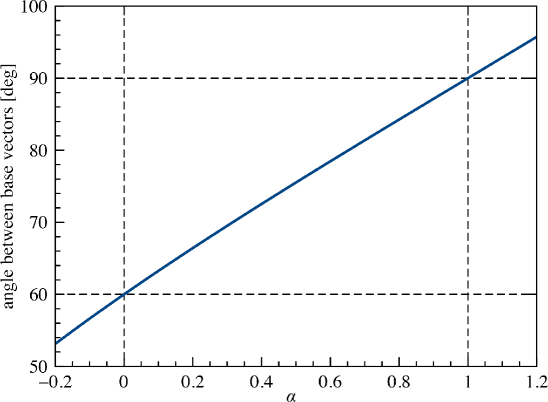
Figure 2: Relationship between the parameter $\alpha$ and the angle between the two base vectors $\vec{b}_{1}$ and $\vec{b}_{2}$.

The shift vector is defined as above with $\beta^{c}=1$ for $\alpha=1$ and $\beta^{h}=\frac{1}{\sqrt{3}}$ for $\alpha=0$. The two sets of distance vectors are given by

$$\vec{r}_{1}(\vec{i})=B(a,\alpha,\gamma)^{\top}\vec{i}\quad\text{and}\quad\vec{r}_{2}(\vec{i})=B(a,\alpha,\gamma)^{\top}\vec{i}+\vec{v}_{s}(a,\beta,\gamma)$$ (21)

We now have a four-parameter space $(a,\alpha,\beta,\gamma)$ as a minimum set of parameters to describe the Burgers-Bain transformation. The symmetric Gram matrix for $B(a,\alpha,\gamma)$ becomes,

$$G(a,\alpha,\gamma)=B(a,\alpha,\gamma)B(a,\alpha,\gamma)^{\top}=a^{2}\begin{pmatrix}1&\omega_{1}(\alpha)&0\\ \omega_{1}(\alpha)&\omega_{2}(\alpha)&0\\ 0&0&\gamma^{2}\end{pmatrix}=a^{2}S_{3}(\alpha,\gamma)$$ (22)

with $\omega_{2}(\alpha)=\omega^{2}_{1}+\omega^{2}_{3}=1$ in our case. The volume of the hexagonal unit cell then is,

$$V(a,\alpha,\gamma)=\sqrt{\text{det}G(a,\alpha,\gamma)}=a^{3}\gamma\sqrt{\omega_{2}(\alpha)-\omega_{1}(\alpha)^{2}}=a^{3}\gamma\omega_{3}(\alpha)=\frac{a^{3}\gamma}{2}\sqrt{(1+\alpha)(3-\alpha)}$$ (23)

This results in a packing density compared to spheres of radius $r$,

$$\rho=\frac{V_{\textrm{sphere}}}{V_{\textrm{hex}}}=\frac{4\pi r^{3}}{3a^{3}\gamma}\frac{2}{\omega_{3}(\alpha)}$$ (24)

where we considered that we have two spheres in the unit cell. This gives $\rho_{\text{bcc}}=\frac{\sqrt{3}}{8}\pi$ (for $\alpha=1$, $\gamma=1$ and $r=\frac{|\vec{v}^{c}|}{2}=\frac{\sqrt{3}}{4}a$), $\rho_{\text{fcc}}=\frac{\sqrt{2}}{6}\pi$ (for $\alpha=1$, $\gamma=\sqrt{2}$ and $r=\frac{1}{2}a$), and $\rho_{\text{hcp}}=\frac{\sqrt{2}}{6}\pi$ (for $\alpha=0$, $\gamma=\sqrt{\frac{8}{3}}$ and $r=\frac{1}{2}a$). We note that $\omega_{2}(\alpha)-\omega_{1}(\alpha)^{2}>0$ for $\alpha\in(-1,3)$.

It is now clear that the martensitic transition is described by shearing of the A-layer, related mainly to the parameter $\alpha$, and a change in angle between the two basis vectors $\vec{b}_{1}$ and $\vec{b}_{2}$ together by a sliding of the B-layer in direction orthogonal to the $\vec{b}_{1}$ and $\vec{b}_{3}$ vectors and additional changes in the crystal parameters $a$ and $\gamma$ (or $c$). This is demonstrated schematically in Figure 3. We note that the Burgers path maintains the symmetry of a primitive monoclinic cell (space group $mP$).

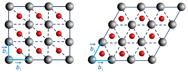
Figure 3: The shearing in the A-layer (grey spheres, change of angle between $\vec{b}_{1}$ and $\vec{b}_{2}$) of the base hexagonal plane and sliding of the B-layer (red spheres, sitting at $\gamma/2$ above the A-layer) in the Burgers transformation. Left: bcc lattice with $\angle(\vec{b}_{1},\vec{b}_{2})=90^{\circ}$ and $\gamma=1$ or fcc lattice with $\gamma=\sqrt{2}$. Right: hcp structure with $\angle(\vec{b}_{1},\vec{b}_{2})=60^{\circ}$ and $\gamma=\sqrt{\frac{8}{3}}$.

We briefly summarize. For the Burgers transformation we reduced the, in principle, nine-parameter space (6 lattice constants for the Bravais lattice plus 3 parameters for the Wyckoff positions of the middle layer) for a bi-lattice to a four-parameter space $(a,\alpha,\beta,\gamma)$, where $\alpha\in(-1,3)$ is the important parameter (our reaction coordinate) describing the Burgers-Bain phase transition. All other parameters $a,\beta,\gamma$ have to be optimized along the transformation path. We expect approximately the following parameter range for $\alpha\in[0,1]$: $a\in[a_{\text{hcp}},a_{\text{bcc}}]$, $\beta\in[\frac{1}{\sqrt{3}},1]$ and $\gamma\in[1,\sqrt{\frac{8}{3}}]$. For the Bain transformation the originally introduced distortion parameter $A$ in Ref. Burrows, Cooper, and Schwerdtfeger, 2021a is simply related to the parameter $\gamma$ by $A=\gamma^{2}/2$, and similarly the nearest neighbor distance in the cuboidal lattice is given by $r_{NN}=\frac{a}{2}\sqrt{2+\gamma^{2}}$.Jerabek, Burrows, and Schwerdtfeger (2022); Robles-Navarro, Jerabek, and Schwerdtfeger This implies that at $\alpha=1$ the transformation from fcc to bcc is described mainly through the parameter $\gamma$.

II.2 Quadratic forms and functions for the lattice sums

Lattice sums have a long history and are usually based on quadratic functions. For inverse power potentials $V(r)=r^{-2s}$ such as the Lennard-Jones potential or the Madelung constant for Coulomb potentials are related to so-called Epstein zeta functions.Borwein et al. (2013); Madelung (1918); Jones and Ingham (1925) For the cuboidal Bain transformation the associated lattice sums were already described in our previous papers Burrows, Cooper, and Schwerdtfeger (2021a, b). For the more general Burgers-Bain transformation we need to introduce two lattice sums for all the distances in a bi-lattice. We first introduce the quadratic form $Q_{A}$ involving only atoms in the base A-layer,

$$Q_{A}(\vec{i},\alpha,\gamma)=\vec{i}^{\top}S_{3}(\alpha,\gamma)\vec{i}=a^{-2}\vec{i}^{\top}G(a,\alpha,\gamma)\vec{i}=i_{1}^{2}+2\omega_{1}(\alpha)i_{1}i_{2}+\omega_{2}(\alpha)i_{2}^{2}+\gamma^{2}i_{3}^{2}$$ (25)

with the associated lattice sum

$$H^{h}_{A}(s,\alpha,\gamma)={\sum_{\vec{i}\in\mathbb{Z}^{3}}}^{{}^{\prime}}\frac{1}{(\vec{i}^{\top}S_{3}(\alpha,\gamma)\vec{i})^{s}}$$ (26)

The prime notation at the sum indicates that we avoid the term $i_{1}=i_{2}=i_{3}$ in the summation. This lattice sum can be re-expressed in terms of a fast converging Bessel function Terras (1973); Burrows et al. (2020) described in detail in Appendix A.

For the second lattice sum we need the quadratic function for the distances between the A- and B-layer atoms derived from Eq. (21),

$$Q_{B}(\vec{i},\alpha,\beta,\gamma) =a^{-2}\left(\vec{i}^{\top}B(a,\alpha,\gamma)+\vec{v}_{s}^{\top}(\beta)\right)\left(B(a,\alpha,\gamma)^{\top}\vec{i}+\vec{v}_{s}(\beta)\right)$$ (27)

$$=a^{-2}\left[\vec{i}^{\top}G(a,\alpha,\gamma)\vec{i}+2\vec{i}^{\top}B(a,\alpha,\gamma)\vec{v}_{s}(\beta,\gamma)+|\vec{v}_{s}(\beta,\gamma)|^{2}\right]$$

$$=(i_{1}+i_{2}\omega_{1}(\alpha)+\tfrac{1}{2})^{2}+(i_{2}\omega_{3}(\alpha)+\tfrac{\beta}{2})^{2}+\gamma^{2}(i_{3}+\tfrac{1}{2})^{2}$$

where $\omega_{1}(\alpha)$ and $\omega_{3}(\alpha)$ have already been defined. The corresponding lattice sum becomes

$$H^{h}_{B}(s,\alpha,\beta,\gamma)=\sum_{\vec{i}\in\mathbb{Z}^{3}}\frac{1}{Q_{B}(\vec{i},\alpha,\beta,\gamma)^{s}}$$ (28)

Both lattice sums are absolute convergent for finite $s>\frac{3}{2}$ with a simple pole at $s=\frac{3}{2}$, but can be analytically continued for $s<\frac{3}{2}$. However, for $s\rightarrow\infty$ the lattice sum $H^{h}_{B}\rightarrow\infty$ for the bcc lattice. This can be understood from the fact that some terms in $Q_{B}(\vec{i}$ for $(i_{1},i_{2},i_{3})\in[-1,1]$ can become smaller than 1 in our definition of the lattice sum. This divergence of the lattice sum for $s\rightarrow\infty$ will be compensated by the optimized lattice constant $a$ obtained from a Lennard-Jones potential as discussed further below, but this results in a $(0\times\infty)$ case for $s\rightarrow\infty$. It is therefore far more convenient to avoid such divergences by re-scaling the lattice constant such that $a=r_{\text{bc}}/f(\beta,\gamma)$, where $f(\beta,\gamma)=a^{-1}|\vec{v}_{s}|$ becomes part of the lattice sum assuring convergence to a finite value for $s\rightarrow\infty$, and $r_{\text{bc}}$ is the length of the vector $\vec{v}_{s}$ from the atom at the base layer A to the nearest body-centered atom in layer B. We now redefine the two lattice sums such that they behave well in the limit $s\rightarrow\infty$,

$$L^{h}_{A}(s,\alpha,\beta,\gamma)=f(\beta,\gamma)^{s}H^{h}_{A}(s,\alpha,\gamma)=f(\beta,\gamma)^{s}{\sum_{\vec{i}\in\mathbb{Z}^{3}}}^{{}^{\prime}}\frac{1}{(\vec{i}^{\top}S_{3}(\alpha,\gamma)\vec{i})^{s}}$$ (29)

and

$$L^{h}_{B}(s,\alpha,\beta,\gamma)=f(\beta,\gamma)^{s}H^{h}_{B}(s,\alpha,\beta,\gamma)=f(\beta,\gamma)^{s}\sum_{\vec{i}\in\mathbb{Z}^{3}}\frac{1}{Q_{B}(\vec{i},\alpha,\beta,\gamma)^{s}}$$ (30)

with

$$f(\beta,\gamma)=a^{-2}|\vec{v}_{s}(\beta,\gamma)|^{2}=a^{-2}r_{\text{bc}}^{2}=\frac{1}{4}\left(1+\beta^{2}+\gamma^{2}\right)$$ (31)

This ensures that the bcc lattice sum is identical to the one defined originally by Lennard-Jones and Ingham Jones and Ingham (1925). The total lattice sum is then given by

$$L^{h}(s,\alpha,\beta,\gamma)=L^{h}_{A}(s,\alpha,\gamma)+L^{h}_{B}(s,\alpha,\beta,\gamma)$$ (32)

Both lattice sums can be expressed in terms of fast converging series involving Bessel functions as derived in Appendix A. We note that it is sufficient to take just the sum of the two layer contributions $L^{h}_{A}+L^{h}_{B}$ as in our definition of the bi-lattice each atom is equivalent to all the others, i.e. they have the same surrounding. This can also be seen from a more general formula for Barlow packings.Schwerdtfeger et al. (2024)

II.3 Lattice sums for the special cases of hcp, fcc and bcc

For the hcp structure we set $\alpha=0$, $\beta=\frac{1}{\sqrt{3}}$ and $\gamma=\sqrt{\frac{8}{3}}$ leading to $\omega_{1}=\frac{1}{2}$, $\omega_{2}=1$, $\omega_{3}=\frac{\sqrt{3}}{2}$ and $f(\beta,\gamma)=1$, and we get

$$L^{\text{hcp}}_{A} ={\sum_{\vec{i}\in\mathbb{Z}^{3}}}^{{}^{\prime}}\left(i_{1}^{2}+i_{1}i_{2}+i_{2}^{2}+\tfrac{8}{3}i_{3}^{2}\right)^{-s}$$ (33)

$$L^{\text{hcp}}_{B} =\sum_{\vec{i}\in\mathbb{Z}^{3}}\left((i_{1}+\tfrac{1}{2}i_{2}+\tfrac{1}{2})^{2}+(\tfrac{\sqrt{3}}{2}i_{2}+\tfrac{1}{2\sqrt{3}})^{2}+\tfrac{8}{3}(i_{3}+\tfrac{1}{2})^{2}\right)^{-s}$$

$$=\sum_{\vec{i}\in\mathbb{Z}^{3}}\left((i_{1}+\tfrac{1}{3})^{2}+(i_{2}+\tfrac{1}{3})^{2}+(i_{1}+\tfrac{1}{3})(i_{2}+\tfrac{1}{3})+\tfrac{8}{3}(i_{3}+\tfrac{1}{2})^{2}\right)^{-s}$$

These are exactly the lattice sums as shown in Refs. Bell and Zucker, 1976; Burrows et al., 2020; Burrows, Cooper, and Schwerdtfeger, 2023.

For bcc we set $\alpha=1$, $\beta=1$ and $\gamma=1$ leading to $\omega_{1}=0$, $\omega_{2}=1$, $\omega_{3}=1$, and $f(\beta,\gamma)=3/4$ we get

$$L^{\text{bcc}}_{A} =\left(\frac{3}{4}\right)^{s}{\sum_{\vec{i}\in\mathbb{Z}^{3}}}^{{}^{\prime}}\left(i_{1}^{2}+i_{2}^{2}+i_{3}^{2}\right)^{-s}$$ (34)

$$L^{\text{bcc}}_{B} =3^{s}\sum_{\vec{i}\in\mathbb{Z}^{3}}\left((2i_{1}+1)^{2}+(2i_{2}+1)^{2}+(2i_{3}+1)^{2}\right)^{-s}$$

These are identical to the ones given by Lennard-Jones and Ingham Jones and Ingham (1925) and used in Ref. Burrows et al., 2020 for various Bessel function expansions.

For fcc we set $\alpha=1$, $\beta=1$ and $\gamma=\sqrt{2}$ leading to $\omega_{1}=0$, $\omega_{2}=1$, $\omega_{3}=1$, and $f(\beta,\gamma)=1$ we get

$$L^{\text{fcc}}_{A} ={\sum_{\vec{i}\in\mathbb{Z}^{3}}}^{{}^{\prime}}\left(i_{1}^{2}+i_{2}^{2}+2i_{3}^{2}\right)^{-s}$$ (35)

$$L^{\text{fcc}}_{B} =\sum_{\vec{i}\in\mathbb{Z}^{3}}\left((i_{1}+\tfrac{1}{2})^{2}+(i_{2}+\tfrac{1}{2})^{2}+2(i_{3}+\tfrac{1}{2})^{2}\right)^{-s}$$

This can be brought into a more familiar form discussed in Ref. Burrows et al., 2020 (see Appendix C),

$$L^{\text{fcc}}_{A}+L^{\text{fcc}}_{B}=2^{s-1}{\sum_{\vec{i}\in\mathbb{Z}^{3}}}^{{}^{\prime}}\left[1+(-1)^{i_{1}+i_{2}+i_{3}}\right]\left(i_{1}^{2}+i_{2}^{2}+i_{3}^{2}\right)^{-s}\\$$ (36)

II.4 The Lennard-Jones cohesive energies for the lattices along the fcc to hcp transition path

The cohesive energy for the hexagonal-cuboidal structures for a general $(n,m)$ LJ potential can be expressed in terms of lattice sums and is given by the expressionJones and Ingham (1925); Schwerdtfeger et al. (2006); Schwerdtfeger, Burrows, and Smits (2021)

$$E_{\text{LJ}}^{\text{coh}}(n,m,a,\alpha,\beta,\gamma)=\frac{\epsilon nm}{2(n-m)}\;\left[\frac{L^{h}(\frac{n}{2},\alpha,\beta,\gamma)}{n}\left(\frac{r_{e}}{r_{\text{bc}}}\right)^{n}-\frac{L^{h}(\frac{m}{2},\alpha,\beta,\gamma)}{m}\left(\frac{r_{e}}{r_{\text{bc}}}\right)^{m}\right]$$ (37)

where the distance from the base to the body-centered atom is related to the lattice constant $r_{\text{bc}}=a/f(\beta,\gamma)$ as already mentioned. The expression for the lattice sum $L^{h}(s,\alpha,\beta,\gamma)$ is taken from Eq. (32) and the corresponding Bessel function expansions we used in our work are given in Appendix A. As these Bessel sum expansions are fast converging series, they can easily be obtained to arbitrary computer precision, i.e. to double precision accuracy within a few seconds of computer time.

In order to discuss the behavior for the LJ potential with varying $a,\alpha,\beta,\gamma$ parameters we eliminate the parameter $a$ to save computer time in our optimizations. Here we first calculate the minimum cohesive energy with respect to the lattice parameter $a$ for fixed set of $\alpha,\beta,\gamma$ values. For this follow the procedure in Ref. Burrows, Cooper, and Schwerdtfeger, 2021b and get from $\partial E_{\textrm{LJ}}^{\textrm{coh}}/\partial a=0$ the minimum lattice parameter,

$$a^{*}_{\text{min}}(\gamma)=\frac{a_{\text{min}}(\alpha,\beta,\gamma)}{r_{e}}=\frac{1}{f(\beta,\gamma)}\left(\frac{L^{h}(\frac{n}{2},\alpha,\beta,\gamma)}{L^{h}(\frac{m}{2},\alpha,\beta,\gamma)}\right)^{\tfrac{1}{n-m}}\,,$$ (38)

and the * indicates that reduced (or dimensionless) units are used. We can then evaluate the cohesive energy at $a^{*}_{\text{min}}$ and get,

$$E_{nm}^{*}(\alpha,\beta,\gamma)=E_{\text{LJ}}^{\text{coh}}(n,m,a^{*}_{\text{bc,min}},\alpha,\beta,\gamma)/\epsilon=-\frac{1}{2}\left[\frac{L^{h}(\frac{m}{2},\alpha,\beta,\gamma)^{n}}{L^{h}(\frac{n}{2},\alpha,\beta,\gamma)^{m}}\right]^{\tfrac{1}{n-m}}\;.$$ (39)

We therefore have to deal only with the three-parameter space $\alpha,\beta,\gamma$ for fixed exponents $(n,m)$. As $\alpha$ is fixed to map out the Burgers path, we only have to optimize $E_{nm}^{*}$ with respect to both $\beta$ and $\gamma$ using a 2D Newton-Raphson procedure as outlined in Appendix D. We chose the interval $\alpha\in[-0.2,1.2]$ in steps of $\Delta\alpha=0.05$ for the Burgers path. For the following we omit the * notation, i.e. all quantities are in reduced (dimensionless) units unless otherwise stated.

The validity of using (39) instead of (37) has been checked by computation which show that we obtain the same results for the extreme points (maxima and minima) and the minimum energy Burgers path. This is perhaps not surprising as we have $\partial E_{nm}/\partial a=0$ and $\partial E_{nm}/\partial\gamma=0$ for the minimum energy path. Thus, by performing the derivative $\partial E_{nm}/\partial a=0$ and considering $\partial L^{h}(\frac{n}{2},\alpha,\beta,\gamma)/\partial a=0$ in (37) we can easily prove by substituting $\partial a=-a\gamma^{-1}\partial\gamma$ that (39) is valid. For the area around the Burgers path where this condition may not hold we obtain rather small deviations from the exact solution (37). Here, the situation is similar to the hcp case discussed before.Burrows, Cooper, and Schwerdtfeger (2023)

III Results and Discussions

By changing step-wise the parameter $\alpha$ from $-0.2$ to $1.2$ we end up with the fcc structure at $\alpha=1$ and $\gamma=\sqrt{2}$ for all LJ potentials considered. Using the reverse path starting from bcc one goes steeply uphill. We therefore focus first our attention on the hcp$\rightarrow$fcc Burgers transformation and then discuss the connection to the bcc phase through the Bain transformation.

III.1 The hcp$\leftrightarrow$fcc Burgers transformation

The optimized lattice parameters $a_{\text{min}}$ are shown in Figure 4 as a function of the distortion parameter $\alpha$ for various LJ potentials. For the interval $\alpha\in[0,1]$ we always have $a\leq r_{\text{bc}}$. For both ideal hcp and fcc we have $a_{\text{min}}=r_{\text{bc,min}}$ because $f(\beta,\gamma)=1$ in both cases. The small difference between $a_{\text{min}}$ and $r_{\text{bc,min}}$ shown in Table 1 comes from the fact that $\gamma$ deviates slightly from the ideal value of $\sqrt{\frac{8}{3}}$ for the LJ potentials. As can be further seen, the lattice parameter is more dependent on the choice of the exponents $n$ and $m$ of the LJ potential than on $\alpha$ itself. This becomes even more evident when we choose the distance $r_{\text{bc}}$ from the base atom to the body-centered atom instead, which remains almost constant over the whole range of $\alpha$ values. Especially for the $(30,12)$-LJ potential $r_{\text{bc}}\approx 1$ close to the kissing hard sphere model where we have $r_{\text{bc}}=1$. In fact, analyzing the minimum distances even further, we get the kissing number $\kappa=12$ for the two points $\alpha=0,\gamma=\sqrt{\frac{8}{3}}$ and $\alpha=1,\gamma=1$ as expected. However, around the TS state we have $\kappa=4$ for the interval $\alpha\in(0,\alpha_{k}$, $\alpha_{k}$ we have $\kappa=6$, and $\kappa=2$ for the interval $\alpha\in(\alpha_{k},1)$ as listed in Table 1 for the various LJ potentials. $\alpha_{k}$ is close to $\frac{1}{2}$.

The optimized lattice parameters $\beta$ and $\gamma$ are shown in Figure 5 as a function of the distortion parameter $\alpha$. The parameter $\beta$, responsible for the sliding of the middle B-layer, is increasing monotonically in an almost linear fashion from $1/\sqrt{3}$ at $\alpha=0$ to 1 at $\alpha=1$ as we expect. This implies a smooth shift of the B-layer for the Burgers transformation from hcp to fcc. The parameter $\gamma$, which for example describes also the Bain transformation, shows a more interesting behavior. There is a slight increase from the value of $\gamma=\sqrt{8/3}$ for the hcp structure with a maximum between $\alpha=0$ and $\alpha=0.2$, followed by the expected decrease to $\gamma=\sqrt{2}$ at $\alpha=1$ for the fcc structure. This will influence the volume and the packing density as can be seen from Eqs. (23) and (24). We note that the hcp structure slightly distorts from the ideal $\gamma=\sqrt{8/3}$ value as discussed in detail before,Burrows, Cooper, and Schwerdtfeger (2023) see Table 1.

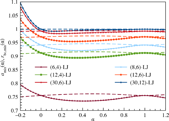
Figure 4: Optimized minimum lattice parameters as a function of the distortion parameter $\alpha$ for various selected $(n,m)$-LJ potentials. The solid lines show the distances between nearest neighbors in the base layer ($a=|\vec{b}_{1}|$), while the dashed lines show the optimized distances from the base to the body-centered atom ($r_{\text{bc}}=|\vec{v}_{s}|$), see Figure 1.

Parameter	$(6,4)$	$(8,6)$	$(12,4)$	$(12,6)$	$(30,6)$	$(30,12)$
minima
$a_{\text{min}}^{\text{hcp}}(\alpha=0)$	0.75523963	0.94115696	0.91206706	0.97127386	0.99229244	0.99939864
$r_{\text{bc,min}}^{\text{hcp}}(\alpha=0)$	0.75533453	0.94108456	0.91203445	0.97118272	0.99225828	0.99938521
$E_{nm}^{\text{hcp}}(\alpha=0)$	-38.9325327	-10.4019067	-18.30985366	-8.61107046	-7.57167198	-6.11058661
$\delta_{nm}^{\text{hcp}}(\alpha=0)$	0.00030779	-0.00018844	-0.00008759	-0.00022986	-0.00008431	-0.00003291
$a_{\text{min}}^{\text{fcc}}(\alpha=1)$	0.75527318	0.94112001	0.91205036	0.97123369	0.99227815	0.99939381
$\Delta E_{nm}^{\text{fcc}}(\alpha=1)$	-0.00167052	0.00065426	0.00053138	0.00087030	0.00063934	0.00034707
$a_{\text{min}}^{\text{cub2}}(\alpha=1)$	0.84952560	1.08593491	1.06151441	1.14235260	1.20025739	1.21772324
$r_{\text{bc,min}}^{\text{cub2}}(\alpha=1)$	0.73571075	0.92022759	0.89393191	0.95447928	0.98606235	0.99654594
$\gamma^{\text{cub2}}(\alpha=1)$	1	0.93401642	0.91472620	0.89022278	0.83649731	0.82395744
$\Delta E_{nm}^{\text{cub2}}(\alpha=1)$	0.29641379	0.24620888	0.45584326	0.34906107	0.58211318	0.76315575
TS Burgers
$\alpha^{\#}$	0.50124827	0.50070620	0.50055491	0.50036605	0.50007315	0.49998534
$a_{\text{min}}^{\#}$	0.73561911	0.92214149	0.89552993	0.95622314	0.98638714	0.99664997
$r_{\text{bc,min}}^{\#}$	0.76148854	0.94610839	0.91637703	0.97463898	0.99337015	0.99965780
$\beta^{\#}$	0.84563200	0.82802883	0.82241205	0.81445956	0.78931350	0.78087408
$\gamma^{\#}$	1.60349255	1.58902301	1.58494120	1.57867371	1.56007043	1.55383900
$\Delta E_{nm}(\alpha^{\#})$	0.63868037	0.34878984	0.59775652	0.41488952	0.59694720	0.76650812
$\Delta V[\%]$	1.45105875	2.35271163	2.73068082	3.15510867	4.92065604	5.51004680
$\alpha_{k}$	0.52877	0.51028	0.50911	0.50408	0.49990	0.49905
TS Bain
$a_{\text{min}}^{\#}$	0.84587206	1.06148905	1.03057025	1.09911882	1.13483878	1.14700157
$r_{\text{bc,min}}^{\#}$	0.73573887	0.91927648	0.89250002	0.95186482	0.95186482	0.99333250
$\Delta E_{nm}(\alpha^{\#})$	0.29644955	0.24972893	0.47009499	0.37377855	0.77263663	1.17257580

Table 1: Optimized parameters for minima and transition states (TS) for various $(n,m)$-LJ potentials. TS properties for the Burgers ($\partial E_{nm}/\partial\alpha=0$) and Bain paths ($\partial E_{nm}/\partial\gamma=0$) are indicated by a $\#$ symbol. For the minimum structures we get exactly $\alpha=0$ and $\beta=1/\sqrt{3}$ for hcp and $\alpha=1$, $\beta=1$ and $\gamma=\sqrt{2}$ for fcc. For hcp obtain a slight deviation from the ideal $\gamma$ value is obtained expressed by $\delta_{nm}(\alpha=0)=\gamma_{nm}^{\text{opt}}(\alpha=0)-\sqrt{8/3}$. cub2 indicates the second cuboidal structure, e.g. bcc if $\alpha=1$, $\beta=1$ and $\gamma=1$. For fcc we have $a_{\text{min}}^{\text{fcc}}(\alpha=1)=r_{\text{bc,min}}^{\text{fcc}}(\alpha=1)$. $\Delta E_{nm}(\alpha^{\#})$ for the Burgers path is taken relative to the hcp structure. The volume increase $\Delta V[\%]$ at the transition point of the Burgers path relative to the fcc structure is defined as $100\{V(\alpha^{\#})-V^{\text{fcc}}\}/V^{\text{fcc}}$. $\alpha_{k}$ defines the point on the Burger’s path where the kissing number changes from 4 to 2 (see text). For the Bain path TS we have $\alpha=1$ and $\beta=1$, which is located at $\gamma=1$ except for the (6,4)-LJ potential for which we get $\gamma^{\#}=$1.01301670. $\Delta E_{nm}(\alpha^{\#})$ for the Bain path are relative to the fcc structure.

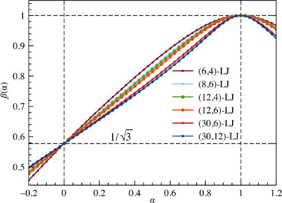
(a) (b)

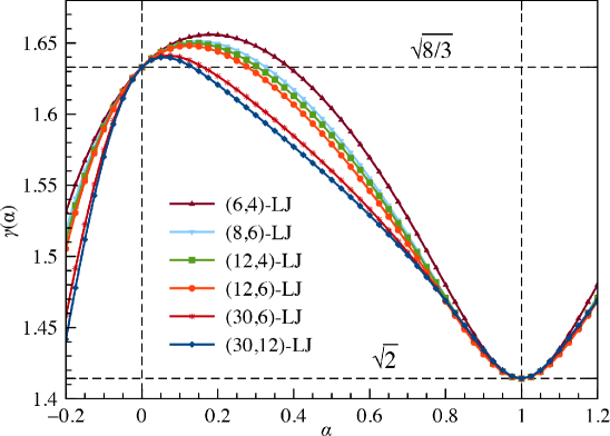
Figure 5: The optimized parameter (a) $\beta$ and (b) $\gamma$ as a function of the distortion parameter $\alpha$ for various selected $(n,m)$-LJ potentials.

Figure 6(a) shows the volume as a function of the distortion parameter $\alpha$. As expected, a volume increase is required for the hcp$\leftrightarrow$fcc transition along the Burgers path with a maximum in volume located close to midpoint at $\alpha=0.5$. The percentage volume increase at this transition state is largest for the $(30,12)$-LJ potential (see Table 1), which is close to the kissing hard-sphere model (KHS). It is difficult to estimate the KHS limit for the volume increase as we do not have an exact value for $\gamma$ at $\alpha=0.5$. However, we assume that for the KHS limit transition state we have exactly $\alpha=0.5$ and $a=1$. For example, for the (40,20)-LJ potential we get $\gamma=1.550$ and a relative volume increase of $100\{V(\alpha=0.5)-V^{\text{fcc}}(\alpha=1)\}/V^{\text{fcc}}(\alpha=1)$=6.13 % with $V^{\text{fcc}}(\alpha=1)=\sqrt{2}$ for the KHS limit.

Concerning the packing density we can define as the hard sphere radius $r=\text{min}\{a,a_{c}\}/2$ in Eq. (24). This implies a non-overlapping sphere model with $2r\leq 1$ for the different $n,m$ combinations of the LJ potential. In other words, the sphere radius changes along the Burgers transition path and the packing density is $\rho\leq\frac{\sqrt{2}}{6}\pi$. This is shown in Figure 6. As a second choice, we may allow spheres to overlap and set the radius to a fixed value of $r=\frac{1}{2}$, the radius of a unit sphere. In this case one has to account for the overlap volume to obtain the correct packing density, see discussion on this subject by Iglesias-Ham et al. Iglesias-Ham, Kerber, and Uhler (2014). In any case, the graphs in Figure 6 show that the packing density is reduced along the Burgers path towards the transition state.

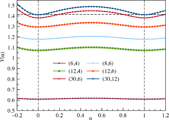
(a) (b)

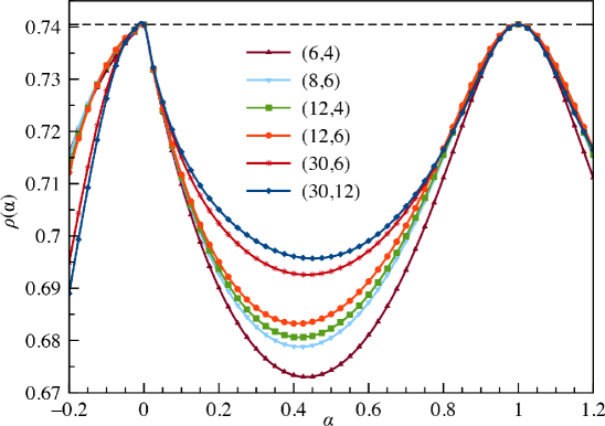
Figure 6: (a) Volume $V$ from (23) and (b) packing density $\rho$ using for the sphere radius (half the nearest neighbor distance) $r=\text{min}\{a,a_{\text{bc}}\}$ in eq. (24) for various selected $(n,m)$-LJ potentials as a function of the distortion parameter $\alpha$. The horizontal lines indicate the hard-sphere limit with for the volume, $V(\alpha=1)=\sqrt{2}$, and the maximum packing density $\rho_{\text{fcc}}=\rho_{\text{hcp}}=\frac{\sqrt{2}}{6}\pi$.

The cohesive energy along the Burgers path is shown in Figure 7. Changing $\alpha$ from $0\rightarrow 1$ and optimization of $\beta$ and $\gamma$ at each step along the path leads straight into the fcc lattice with $\gamma=\sqrt{2}$ and a transition state close to the midpoint of $\alpha=1/2$ for all LJ potentials considered here. For example, for the (12,6)-LJ potential we find the transition state at $\alpha^{\#}=0.50037$ with an energy difference of $\Delta E_{12,6}(\alpha^{\#})=E_{12,6}(\alpha^{\#})-E_{12,6}^{\text{hcp}}=0.41490$, see Table 1. To give this a meaning for real solids, we multiply the energy difference with the most accurate available dissociation energy of $\epsilon=99.351\pm 0.32$ cm^-1 for Ar₂ from relativistic coupled-cluster calculations of Patkowski and Szalewicz,Patkowski and Szalewicz (2010) and obtain for the activation energy to the transition state a value of 41.2 cm^-1 (kcal/mol) compared to the hcp structure. This compares to the experimentally known cohesive energy of solid argon of 7722(11) cm^-1,Schwalbe et al. (1977) i.e. the barrier height is less than 1% of the cohesive energy. Furthermore, the activation energy is smaller than the zero-point vibrational contribution for fcc argon which is 67.4 cm^-1.Schwerdtfeger et al. (2016)

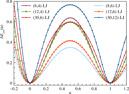
Figure 7: The cohesive energy difference $\Delta E_{nm}(\alpha)=E_{nm}(\alpha)-E_{nm}^{\text{hcp}}(\alpha=0)$ for the Burgers path as a function of the distortion parameter $\alpha$ for various selected $(n,m)$-LJ potentials.

We can also compare with recent molecular dynamics (MD) simulation by Bingxi Li et al.Li et al. (2017) using a (12,6)-LJ potential and 18,000 Ar atoms in a box adjusted to a temperature of $T$=40 K and pressure of $P$= 1 bar. They calculated a barrier height for the enthalpy of $\Delta H^{\#}=16.0\pm 1.0$ cm^-1 (per atom). Even if we adjust for the more accurate dissociation energy of Patkowski and SzalewiczPatkowski and Szalewicz (2010) then given in their paper we get $\Delta H^{\#}=19.2\pm 1.1$ cm^-1. However, at 40K the kinetic energy per atom $E_{\text{kin}}=\frac{3}{2}k_{\text{B}}T$ translates into 41.7 cm^-1 per atom. Hence it is difficult to compare our two very different (static vs. dynamic) methods. Moreover, their MD simulations show an accumulation of defects, stacking disorders and growth of a less ordered structures towards the transition state. They also detected three different phase transition paths. It is, however, difficult to provide a simple picture of the phase transition from such MD simulations, even more so if the simulation cell does not reflect the change in the lattice constants and surface effects can become important without proper periodic boundary conditions. On the contrary, the Burgers path provides a good upper limit for the activation energy in the hcp$\leftrightarrow$fcc transformation, as other paths on such a high-dimensional energy hypersurface requiring a large super-cell treatment may lie below the ideal Burgers path. Interestingly, the volume expansion at the transition state obtained by Bingxi Li et al.Li et al. (2017) of about 2.6% is not too different compared to our value of 3.2%.

The activation energies for the Bain phase transition are usually below the ones for the Burgers path, see Table 1. The highest barrier for the Bain path is obtained by the most repulsive $(30,12)$-LJ potential, as one might expect. Further, the difference in energy between the fcc and hcp structures are very small, i.e. $\Delta E_{nm}=E_{nm}^{\text{hcp}}-E_{nm}^{\text{fcc}}=0.0008703$ for the (12,6)-LJ potential and -0.0016705 for the (6,4)-LJ potential. In the latter case, fcc is more stable compared to hcp. Figure 8 shows the hcp-fcc phase transition line between the two phases where we have $\Delta E_{nm}=0$. Only for very soft long-range potentials becomes the fcc phase more stable compared to the hcp phase. The critical $n_{c},m_{c}$ values for the phase transition line can be fitted to the function

$$m_{c}=3+ae^{-bn_{c}}+\frac{c_{1}}{n_{c}}+\frac{c_{2}}{n_{c}^{2}}+\frac{c_{3}}{n_{c}^{3}}\quad\text{with}\quad n_{c}>5.705$$ (40)

where $a=3.322473067\times 10^{8}$, $b=5.95017115$, $c_{1}=-9.23169654$, $c_{2}=1.73880812\times 10^{2}$ and $c_{3}=-1.89668849\times 10^{2}$ with a coefficient of determination of $R^{2}=0.9998$. For example, for $n_{c}=12$ we get $m_{c}=3.291725434064$, which means that for the $(12,6)$-LJ potential the hcp phase lies energetically below the fcc phase. This was intensively discussed already in the literature Kihara and Koba (1952); Wallace and Patrick (1965); Niebel and Venables (1974); van de Waal (1991); Lotrich and Szalewicz (1997); Schwerdtfeger, Burrows, and Smits (2021), and it was recently shown that for a solid like argon, phonon dispersion is required for the stabilization of the fcc over the hcp phase at 0K.Schwerdtfeger et al. (2016)

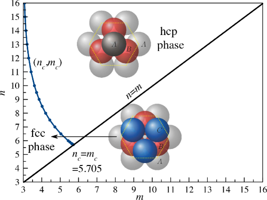
Figure 8: hcp/fcc phase transition line $(n_{c},m_{c})$ for $(n,m)$-LJ potentials fulfilling the condition $\Delta E_{nm}=E_{nm}^{\text{hcp}}-E_{nm}^{\text{fcc}}$.

III.2 The Burgers-Bain transformation

The question arises if there is another direct path from hcp to bcc as suggested for example by Carter and co-workers for iron or lithium Johnson and Carter (2008); Caspersen and Carter (2005). However, the MD simulations by Bingxi Li et al.Li et al. (2017) show no transition to the bcc phase. We note that one can always go from fcc to bcc via a Bain-type transformation as has been discussed for example by our group before for LJ potentials Burrows, Cooper, and Schwerdtfeger (2021b); Schwerdtfeger and Burrows (2022).

In order to shed light into this we decided to scan through the $(\alpha,\gamma)$ parameter space by optimizing $\beta$ at each point. We did not consider the (30,12)-LJ potential as it is close to the kissing hard-sphere limit. As a result, at larger $\gamma$ values we see symmetry breaking effects such that the middle B-layer becomes energetically unstable and by moving either up or down towards one of the A-layers. This movement parallel to the base hexagonal sheet would cost little energy due to the short-range nature of the potential, which makes the optimization of the $\beta$ parameter difficult. Furthermore, the bcc structure at $\gamma=1$ is a maximum for this potential distorting either to fcc or to another minimum at $\alpha=1$, $\beta=1$ and $\gamma=0.82395744$, cf. Table 1, very close to the ideal acc structure with $\gamma=\sqrt{2/3}$.

The energy hypersurfaces for four different LJ potentials are shown in Figure 9. We can clearly see the minimum energy path (in our limited four-parameter space) from the hcp minimum ($\alpha=0$ and $\gamma\approx\sqrt{8/3}$) on the left to the fcc minimum ($\alpha=1$ and $\gamma=\sqrt{2}$ on the right of the contour plot. We can also see the Bain path at constant $\alpha=1$ from fcc towards the bcc structure $\gamma=1$. It is now clear that the hcp$\rightarrow$bcc minimum energy transition in our model involves two transition states and requires the fcc lattice as an intermediate structure. Concerning the stability of the two different phases we already pointed out that the bcc phase lies always above the fcc structure and is meta-stable only for soft long-range potentials,Schwerdtfeger, Burrows, and Smits (2021) otherwise it becomes unstable and distorts towards the acc structure with smaller $\gamma$ values Burrows, Cooper, and Schwerdtfeger (2021b). It was already mentioned that the kissing number reduces to 8 for the interval $\gamma\in(\sqrt{2},\sqrt{2/3})$, which may explain why this path is energetically lower compared to the Burgers path (except for the potentials with high $n$and $m$ values).

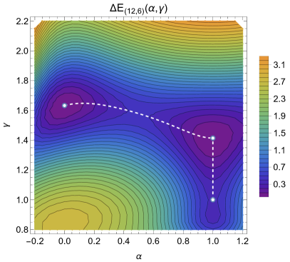
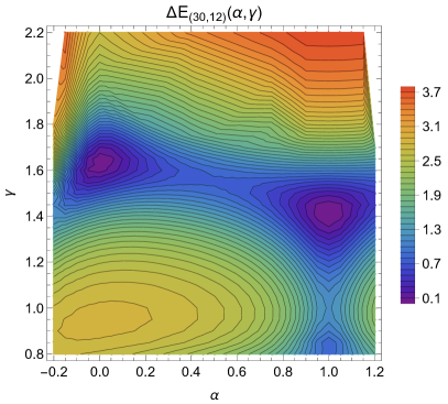
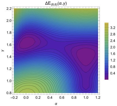
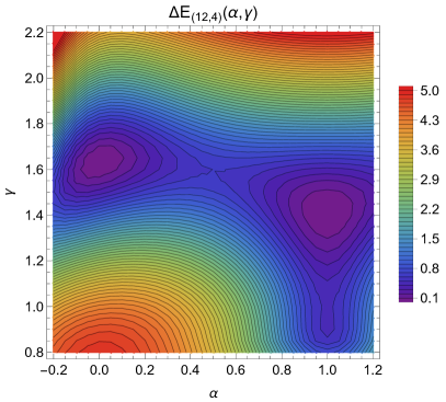
Figure 9: Contour plots for the $(\alpha,\gamma)$ energy hypersurfaces at optimized $\beta$ values for the cohesive energy difference $\Delta E_{nm}(\alpha)=E_{nm}(\alpha)-E_{nm}^{\text{hcp}}(\alpha=0)$ of a $(12,6)$-LJ potential (top left), $(30,12)$-LJ potential (top right), $(8,6)$-LJ potential (bottom left), and $(12,4)$-LJ potential (bottom right). For the $(12,6)$-LJ the minimum Burgers path from hcp ($\alpha=0,\gamma=\sqrt{\frac{8}{3}}$. left minimum) to fcc ($\alpha=0,\gamma=\sqrt{2}$, right minimum) and the minimum Bain path at constant $\alpha=1$ from fcc to bcc $\alpha=1,\gamma=1$ are shown. Note the different energy scales used as shown on the right hand side of the contour plots.

As mentioned already, the minimum energy path is unaffected by the model applied, i.e. using (39) instead of the exact LJ expression (37). As we map the hypersurface in the $(\alpha,\gamma)$ space (39) is also valid. We note a maximum around $\alpha=0.0$ and $\gamma=0.8$, clearly visible in Figure 9. For example, for the (12,6)-LJ potential we obtain $\alpha=0$, $\beta=1/\sqrt{3}$, $a=0.95109476$, $\gamma=0.84836004$ and $\Delta E^{*}=2.77589575$ compared to the hcp minimum structure using (37). These values are identical to the ones obtained before for the hcp lattice,Burrows, Cooper, and Schwerdtfeger (2023) where the cohesive energy with changing $\gamma$ has been studied in detail.

IV Conclusions

We investigated in detail the Burgers-Bain minimum energy path for the hcp$\leftrightarrow$fcc$\leftrightarrow$bcc phase transition for a number of representative $(n,m)$-LJ potentials using exact (to computer precision) lattice summations. For this we expressed the lattice sums in terms of a fast converging Bessel sum series. Our simple phase transition model is currently limited to four parameters describing the change in the base lattice parameters $a$ and $c$, the shear force acting on the hexagonal base plane through the parameter $\alpha$, and the sliding force of the middle layer through the parameter $\beta$. We treated $a$ and $\gamma=c/a$ as independent parameters here,Burrows, Cooper, and Schwerdtfeger (2023) which is computationally most efficient and reasonably accurate. This limited choice of parameters made is possible to gain detailed insight into the Burgers-Bain phase transition. A more detailed study for solid argon under pressure is currently underway. The true minimum energy path might well lie energetically below the ideal Burgers-Bain path involving a different mechanism for the sliding of the hexagonal planes. Moreover, for real systems with strong many-body interactions such as for metallic systems,Schwerdtfeger et al. (2006) the bcc phase might well be directly connected to the hcp phase as for example calculations using density functional theory and the nudged elastic band algorithm for mapping out the minimum energy path for bulk lithium or silver nanowires indicate.Caspersen and Carter (2005); Sun et al. (2022) We point out that a more advanced MD simulation to obtain free energy values at finite temperatures and pressures requires a super-cell treatment with a large set of independent parameters. Nevertheless, we believe that our simple picture can be used to estimate an upper limit of the phase transition activation barrier for real systems applying density functional theory.

V Appendix

Appendix A Bessel function expansions of the lattice sums for the Burgers path

In the following we concentrate on the lattice sums $H^{h}_{A}$ and $H^{h}_{B}$ so we do not have to carry the factor $f(\beta,\gamma)$ along.

A.1 The lattice sum $H^{h}_{A}$

In three dimensions the lattice sum defined through a quadratic form is related to the Epstein zeta function $Z$ by $H_{S_{3}}=2Z_{S_{3}}\left(s\right)$ as discussed by TerrasTerras (1973), where $S_{3}$ is a three-dimensional symmetric and positive definite Gram matrix. The Terras decomposition of the Epstein zeta functionTerras (1973) can be used for any Bravais lattice and an inverse power potential, and has been detailed in our previous paper for cubic lattices,Burrows et al. (2020)

$$Z_{S_{3}}(s) =\frac{\pi\Gamma(s-1)t^{1-s}}{\Gamma(s)\sqrt{\det S_{2}}}\zeta(2s-2)+\frac{p^{\frac{1}{2}-s}\Gamma(s-\frac{1}{2})}{\Gamma(s)}\sqrt{\frac{\pi}{\sigma_{22}}}\zeta(2s-1)+\frac{\zeta(2s)}{\sigma_{22}^{s}}$$ (A.1)

$$+\frac{4\pi^{s}}{\Gamma(s)}\left(\frac{p^{1-2s}}{\sigma_{22}^{1+2s}}\right)^{1/4}\sum_{u,v\in\mathbb{N}}\left(\frac{v}{u}\right)^{s-\frac{1}{2}}\cos\left(\frac{2\pi\sigma_{12}uv}{\sigma_{22}}\right)K_{s-\frac{1}{2}}\left(2\pi uv\sqrt{\frac{p(\alpha)}{\sigma_{22}}}\right)$$

$$+\frac{2\pi^{s}}{\Gamma(s)}\sqrt{\frac{t^{1-s}}{\det S_{2}}}\sum_{\begin{subarray}{c}u\in\mathbb{N}\\ \vec{w}\in\tilde{\mathbb{Z}}^{2}\setminus\{\vec{0}_{2}\}\end{subarray}}\cos\left(2\pi u\vec{w}^{\top}\vec{y}\right)u^{1-s}\left(\vec{w}^{\top}S_{2}^{-1}\vec{w}\right)^{\frac{s-1}{2}}K_{s-1}\left(2\pi u\sqrt{t\vec{w}^{\top}S_{2}^{-1}\vec{w}}\right)$$

Here $S_{3}$ has been block-diagonalized to obtain the $(2\times 2)$ symmetric sub-matrix $S_{2}=(\sigma_{ij})$,

$$S_{3}=\begin{pmatrix}m&\vec{z}^{\top}\\ \vec{z}&S_{2}\end{pmatrix}=\begin{pmatrix}1&\vec{y}^{\top}\\ \vec{0}_{2}&I_{2}\end{pmatrix}\begin{pmatrix}t&\vec{0}_{2}^{\top}\\ \vec{0}_{2}&S_{2}\end{pmatrix}\begin{pmatrix}1&\vec{0}_{2}^{\top}\\ \vec{y}&I_{2}\end{pmatrix}$$ (A.2)

and $\vec{y}$, $\vec{z}$ are simple 2-vectors. This gives the relations,

$$\vec{z}=S_{2}\vec{y}\quad\implies\quad\vec{y}=S_{2}^{-1}\vec{z}$$ (A.3)

and

$$m=t+\vec{y}^{\top}S_{2}\vec{y}\quad\implies\quad t=m-\vec{z}^{\top}S_{2}^{-1}\vec{z}$$ (A.4)

with $t\neq 0$ and

$$S_{2}^{-1}={\rm det}(S_{2})^{-1}\begin{pmatrix}\sigma_{22}&-\sigma_{12}\\ -\sigma_{12}&\sigma_{11}\end{pmatrix}$$ (A.5)

The other parameters and functions are defined as follows,

$$p=\left\{\sigma_{11}-\frac{\sigma_{12}^{2}}{\sigma_{22}}\right\}$$ (A.6)

The modified Bessel function is defined as

$$K_{\nu}(x)=\frac{1}{2}\int_{0}^{\infty}u^{\nu-1}{\rm exp}\left\{-x\left(u+u^{-1}\right)/2\right\}du\quad{\rm for}\quad|{\rm arg}(x)|<\tfrac{1}{2}\pi$$ (A.7)

with $K_{\nu}(x)=K_{-\nu}(x)$,Glasser et al. (2012) The higher-order Bessel functions can be successively reduced to lower order Bessel functions by

$$K_{\nu}(x)=\frac{2(\nu-1)}{x}K_{\nu-1}(x)+K_{\nu-2}(x)$$ (A.8)

and all what remains to be evaluated are the Bessel functions $K_{1}$, $K_{0}$ and $K_{\tfrac{1}{2}}$. Further, for half-integer orders of the Bessel function we can use the equation

$$K_{\tfrac{1}{2}}(x)=K_{-\tfrac{1}{2}}(x)=\sqrt{\frac{\pi}{2x}}e^{-x}$$ (A.9)

The relation for the $\Gamma$-functions is

$$\Gamma(x+1)=x\Gamma(x)$$ (A.10)

For the symmetric matrix $S_{3}$ we take

$$S_{3}(\alpha,\gamma)=\begin{pmatrix}\gamma^{2}&0&0\\ 0&1&\omega_{1}(\alpha)\\ 0&\omega_{1}(\alpha)&\omega_{2}(\alpha)\end{pmatrix}\quad\text{and}\quad S_{2}(\alpha,\gamma)=\begin{pmatrix}1&\omega_{1}(\alpha)\\ \omega_{1}(\alpha)&\omega_{2}(\alpha)\end{pmatrix}$$ (A.11)

which gives $\vec{y}^{\top}=(0,0)$ and $m=t=\gamma^{2}$. Taking $\sigma_{11}=1,\sigma_{12}(\alpha)=\omega_{1}(\alpha)$, $\sigma_{22}(\alpha)=\omega_{2}(\alpha)$, $p(\alpha)=1-\frac{\omega_{1}(\alpha)^{2}}{\omega_{2}(\alpha)}>0$ and $\det S_{2}(\alpha)=\omega_{2}(\alpha)-\omega_{1}(\alpha)^{2}=\frac{p(\alpha)}{\omega_{2}(\alpha)}>0$ for $\alpha\in[0,1]$, and we get

$$H_{A}^{h}(s) =\frac{2\pi\Gamma(s-1)}{\gamma^{2s-2}\Gamma(s)}\sqrt{\frac{\omega_{2}(\alpha)}{p(\alpha)}}\zeta(2s-2)+\frac{2p(\alpha)^{\frac{1}{2}-s}\Gamma(s-\frac{1}{2})}{\Gamma(s)}\sqrt{\frac{\pi}{\omega_{2}(\alpha)}}\zeta(2s-1)+\frac{2\zeta(2s)}{\omega_{2}(\alpha)^{s}}$$ (A.12)

$$+\frac{8\pi^{s}}{\Gamma(s)}\left(\frac{p(\alpha)^{1-2s}}{\omega_{2}(\alpha)^{1+2s}}\right)^{1/4}\sum_{u,v\in\mathbb{N}}\left(\frac{v}{u}\right)^{s-\frac{1}{2}}\cos\left(\frac{2\pi\omega_{1}(\alpha)uv}{\omega_{2}(\alpha)}\right)K_{s-\frac{1}{2}}\left(2\pi uv\sqrt{\frac{p(\alpha)}{\omega_{2}(\alpha)}}\right)$$

$$+\frac{4\pi^{s}}{\gamma^{s-1}\Gamma(s)}\sqrt{\frac{\omega_{2}(\alpha)}{p(\alpha)}}\sum_{\begin{subarray}{c}u\in\mathbb{N}\\ \vec{w}\in\tilde{\mathbb{Z}}^{2}\setminus\{\vec{0}_{2}\}\end{subarray}}u^{1-s}\left(\vec{w}^{\top}S_{2}^{-1}\vec{w}\right)^{\frac{s-1}{2}}K_{s-1}\left(2\pi\gamma u\sqrt{\vec{w}^{\top}S_{2}^{-1}\vec{w}}\right)$$

and for the inverse $S_{2}$ matrix we have

$$S_{2}^{-1}=\frac{1}{\omega_{2}(\alpha)-\omega_{1}(\alpha)^{2}}\begin{pmatrix}\omega_{2}(\alpha)&-\omega_{1}(\alpha)\\ -\omega_{1}(\alpha)&1\end{pmatrix}$$ (A.13)

A.2 The lattice sum $H^{h}_{B}$

This is the more complicated case, but we can use the expansion derived from Van der Hoff and Benson’s original expression derived from a Mellin transformation and the use of theta functions,van der Hoff and Benson (1953)

$$\sum_{i\in\mathbb{Z}}\left[x^{2}+(i+\zeta)^{2}\right]^{-s} =\frac{\sqrt{\pi}\Gamma(s-\frac{1}{2})}{\Gamma(s)\left|x\right|^{2s-1}}+\frac{4\pi^{s}}{\Gamma(s)}\sum_{n\in\mathbb{N}}\left(\frac{n}{\left|x\right|}\right)^{s-\frac{1}{2}}\cos(2\pi n\zeta)K_{s-\frac{1}{2}}(2\pi n|x|)$$ (A.14)

with $\zeta\in[0,1)$. We rewrite the quadratic function into

$$Q_{B}(i,j,k,\alpha,\beta,\gamma) =\gamma^{2}\left[\gamma^{-2}(i+j\omega_{1}(\alpha)+\tfrac{1}{2})^{2}+\gamma^{-2}(j\omega_{3}(\alpha)+\tfrac{\beta}{2})^{2}+(k+\tfrac{1}{2})^{2}\right]$$ (A.15)

$$=\gamma^{2}\left[\gamma^{-2}x^{2}_{ij}(\alpha,\beta)+(k+\tfrac{1}{2})^{2}\right]$$

and get

$$H_{B}^{h}(s,\alpha,\beta,\gamma) =\sum_{\vec{i}\in\tilde{\mathbb{Z}}^{3}}Q_{B}(\vec{i},\alpha,\beta,\gamma)^{-s}=\frac{\sqrt{\pi}\Gamma\left(s-\frac{1}{2}\right)}{\gamma\Gamma(s)}\sum_{i,j\in\mathbb{Z}}\left|x_{ij}\right|^{1-2s}$$ (A.16)

$$+\frac{4\pi^{s}}{\gamma^{s+\frac{1}{2}}\Gamma(s)}\sum_{i,j\in\mathbb{Z}}\sum_{n\in\mathbb{N}}(-1)^{n}\left(\frac{n}{\left|x_{ij}(\alpha,\beta)\right|}\right)^{s-\frac{1}{2}}K_{s-\frac{1}{2}}\left(\frac{2\pi n|x_{ij}(\alpha,\beta)|}{\gamma}\right)$$

with

$$x_{ij}(\alpha,\beta)^{2}=(i+j\omega_{1}(\alpha)+\tfrac{1}{2})^{2}+(j\omega_{3}(\alpha)+\tfrac{\beta}{2})^{2}$$ (A.17)

One has to avoid $x^{2}_{ij}=0$ for this expansion. For the range of $(\alpha,\beta)$ parameters with $\omega_{1}\in[0,\frac{1}{2}]$, $\omega_{3}\in[\frac{\sqrt{3}}{2},1]$ and $\beta\in[\frac{1}{\sqrt{3}},1]$, one can easily show that $x^{2}_{ij}>0$. This expansion reduces the problem into a fast converging triple sum involving Bessel functions, and into an additional double sum,

$$W(\alpha,\beta)=\sum_{i,j\in\mathbb{Z}}\left\{(i+j\omega_{1}(\alpha)+\tfrac{1}{2})^{2}+(j\omega_{3}(\alpha)+\tfrac{\beta}{2})^{2}\right\}^{\frac{1}{2}-s}$$ (A.18)

which however is slowly convergent for low $s$ values. We therefore use again expansion (A.14) with $\zeta=j\omega_{1}(\alpha)+\tfrac{1}{2}$ and $x=j\omega_{3}(\alpha)+\tfrac{\beta}{2}$ and get

$$W (\alpha,\beta)=\frac{\sqrt{\pi}\Gamma(s-1)}{\Gamma(s-\frac{1}{2})}\sum_{j\in\mathbb{Z}}\frac{1}{|j\omega_{3}(\alpha)+\frac{\beta}{2}|^{2s-2}}$$ (A.19)

$$+\frac{4\pi^{s-\frac{1}{2}}}{\Gamma(s-\frac{1}{2})}\sum_{j\in\mathbb{Z}}\sum_{n\in\mathbb{N}}\left(\frac{n}{|j\omega_{3}(\alpha)+\frac{\beta}{2}|}\right)^{s-1}\cos\left(2\pi n\left[j\omega_{1}(\alpha)+\frac{1}{2}\right]\right)K_{s-1}\left(2\pi n\left|j\omega_{3}(\alpha)+\frac{\beta}{2}\right|\right)$$

The first sum can be turned into a Hurwitz zeta function $h(s,x)$,

$$\sum_{j\in\mathbb{Z}}\frac{1}{|j+\tfrac{\beta}{2\omega_{3}(\alpha)}|^{2s-2}}=h\left(2s-2,\tfrac{\beta}{2\omega_{3}(\alpha)}\right)+h\left(2s-2,1-\tfrac{\beta}{2\omega_{3}(\alpha)}\right)$$ (A.20)

with

$$h(s,x)=\sum_{n\in\mathbb{N}_{0}}\frac{1}{(n+x)^{s}}$$ (A.21)

In summary, the lattice sum $H_{B}$ is

$$H_{B}^{h} (s,\alpha,\beta,\gamma)=\frac{\pi\Gamma(s-1)}{\gamma\Gamma(s)\omega_{3}(\alpha)^{2s-2}}\left[h\left(2s-2,\tfrac{\beta}{2\omega_{3}(\alpha)}+h\left(2s-2,1-\tfrac{\beta}{2\omega_{3}(\alpha)}\right)\right)\right]$$

$$+\frac{4\pi^{s}}{\gamma\Gamma(s)}\sum_{j\in\mathbb{Z}}\sum_{n\in\mathbb{N}}\left(\frac{n}{|j\omega_{3}(\alpha)+\frac{\beta}{2}|}\right)^{s-1}\cos\left(2\pi n\left[j\omega_{1}(\alpha)+\frac{1}{2}\right]\right)K_{s-1}\left(2\pi n\left|j\omega_{3}(\alpha)+\frac{\beta}{2}\right|\right)$$

$$+\frac{4\pi^{s}}{\gamma^{s+\frac{1}{2}}\Gamma(s)}\sum_{i,j\in\mathbb{Z}}\sum_{n\in\mathbb{N}}(-1)^{n}\left(\frac{n}{|x_{ij}(\alpha,\beta)|}\right)^{s-\frac{1}{2}}K_{s-\frac{1}{2}}\left(\frac{2\pi n|x_{ij}(\alpha,\beta)|}{\gamma}\right)$$ (A.22)

A.3 Adding both lattice sums

We can now add both lattice sums $H^{h}_{A}$ and $H^{h}_{B}$

$$H^{h}\left(s,\alpha,\beta,\gamma\right)=g_{0}\left(s,\alpha,\beta,\gamma\right)+\sum_{n=1}^{4}g_{n}\left(s,\alpha,\beta,\gamma\right)$$ (A.23)

with

$$g_{0} \left(s,\alpha,\beta,\gamma\right)=\frac{2\pi\Gamma\left(s-1\right)}{\gamma^{2s-2}\Gamma\left(s\right)}\sqrt{\frac{\omega_{2}(\alpha)}{p(\alpha)}}\zeta(2s-2)+\frac{2p(\alpha)^{\frac{1}{2}-s}\Gamma(s-\frac{1}{2})}{\Gamma(s)}\sqrt{\frac{\pi}{\omega_{2}(\alpha)}}\zeta(2s-1)$$

$$+\frac{2\zeta(2s)}{\omega_{2}(\alpha)^{s}}+\frac{\pi\Gamma\left(s-1\right)}{\gamma\Gamma(s)\omega_{3}(\alpha)^{2s-2}}\left\{h\left(2s-2,\tfrac{\beta}{2\omega_{3}(\alpha)}\right)+h\left(2s-2,1-\tfrac{\beta}{2\omega_{3}(\alpha)}\right)\right\}$$ (A.24)

and each of the following $g_{n}$ terms containing an infinite sum of Bessel functions such that

$$g_{1}\left(s,\alpha\right)=\frac{8\pi^{s}}{\Gamma(s)}\frac{p(\alpha)^{\frac{1-2s}{4}}}{\omega_{2}(\alpha)^{\frac{1+2s}{4}}}\sum_{i,j\in\mathbb{N}}\left(\frac{i}{j}\right)^{s-\frac{1}{2}}\cos\left(\frac{2\pi\omega_{1}(\alpha)ij}{\omega_{2}(\alpha)}\right)K_{s-\frac{1}{2}}\left(2\pi ij\sqrt{\frac{p(\alpha)}{\omega_{2}(\alpha)}}\right)$$ (A.25)

$$g_{2}\left(s,\alpha,\gamma\right)=\frac{4\pi^{s}}{\gamma^{s-1}\Gamma(s)}\sqrt{\frac{\omega_{2}(\alpha)}{p(\alpha)}}\sum_{\begin{subarray}{c}n\in\mathbb{N}\\ \vec{w}\in\tilde{\mathbb{Z}}^{2}\setminus\{\vec{0}_{2}\}\end{subarray}}\left(\frac{\vec{w}^{\top}S_{2}^{-1}\vec{w}}{n^{2}}\right)^{\frac{s-1}{2}}K_{s-1}\left(2\pi n\gamma\sqrt{\vec{w}^{\top}S_{2}^{-1}\vec{w}}\right)$$ (A.26)

$$g_{3}\left(s,\alpha,\beta,\gamma\right) =\frac{4\pi^{s}}{\gamma\Gamma(s)}\sum_{j\in\mathbb{Z}}\sum_{n\in\mathbb{N}}\left(\frac{n}{|j\omega_{3}(\alpha)+\frac{\beta}{2}|}\right)^{s-1}\cos\left(2\pi n\left[j\omega_{1}(\alpha)+\frac{1}{2}\right]\right)\quad$$ (A.27)

$$\times K_{s-1}\left(2\pi n\left|j\omega_{3}(\alpha)+\frac{\beta}{2}\right|\right)$$

$$g_{4}\left(s,\alpha,\beta,\gamma\right)= \frac{4\pi^{s}}{\gamma^{s+\frac{1}{2}}\Gamma(s)}\sum_{i,j\in\mathbb{Z}}\sum_{n\in\mathbb{N}}(-1)^{n}\left(\frac{n}{|x_{ij}(\alpha,\beta)|}\right)^{s-\frac{1}{2}}K_{s-\frac{1}{2}}\left(2\pi n\gamma^{-1}|x_{ij}(\alpha,\beta)|\right)$$ (A.28)

with $p(\alpha)=1-\frac{\omega_{1}(\alpha)^{2}}{\omega_{2}(\alpha)}>0$ as defined before.

For computational purposes we need to treat the first three Bessel sums more efficiently. For the first Bessel sum $g_{1}$ appearing in $H^{h}_{A}$ we use permutation symmetry between $i$ and $j$ and get,

$$g_{1}\left(s,\alpha\right) =\frac{8\pi^{s}}{\Gamma(s)}\frac{p(\alpha)^{\frac{1-2s}{4}}}{\omega_{2}(\alpha)^{\frac{1+2s}{4}}}\sum_{i\geq j\in\mathbb{N}}\left(1-\tfrac{1}{2}\delta_{ij}\right)\left[\left(\frac{i}{j}\right)^{s-\frac{1}{2}}+\left(\frac{j}{i}\right)^{s-\frac{1}{2}}\right]\cos\left(\frac{2\pi\omega_{1}(\alpha)ij}{\omega_{2}(\alpha)}\right)$$

$$\times K_{s-\frac{1}{2}}\left(2\pi ij\sqrt{\frac{p(\alpha)}{\omega_{2}(\alpha)}}\right)$$ (A.29)

where $\delta_{ij}$ is the Kronecker symbol. The sum $g_{3}$ for $H^{h}_{B}$ can be dealt with in a similar way,

$$g_{3}(s,\alpha,\beta,\gamma) =\frac{4\pi^{s}}{\gamma\Gamma(s)}\sum_{i\in\mathbb{N}}\left(-1\right)^{i}\left(\frac{2i}{\beta}\right)^{s-1}K_{s-1}\left(\pi\beta i\right)+\frac{4\pi^{s}}{\gamma\Gamma(s)}\sum_{i,j\in\mathbb{N}}(-1)^{i}\cos\left(2\pi\omega_{1}(\alpha)ij\right)$$

$$\times\sum_{k\in\{-1,+1\}}\left(\frac{i}{\left(j\omega_{3}(\alpha)+\frac{1}{2}k\beta\right)}\right)^{s-1}K_{s-1}\left(2\pi i\left(j\omega_{3}(\alpha)+\frac{1}{2}k\beta\right)\right)$$ (A.30)

and we used cos$(x+n\pi)=(-1)^{n}$cos$(x)$ and remember that $\beta>0$ and $j\omega_{3}(\alpha)>\frac{1}{2}k\beta$. The first single sum is related to the infinite sum in (A.14) and is one of the most common Bessel function series in the literature Fucci and Kirsten (2015).

For the triple sum $g_{2}$ we simply use the fact that $S_{2}^{-1}$ is a symmetric matrix and get,

$$g_{2}\left(s,\alpha,\gamma\right) =\frac{4\pi^{s}}{\gamma^{s-1}\Gamma(s)}\sqrt{\frac{\omega_{2}(\alpha)}{p(\alpha)}}\sum_{n\in\mathbb{N}}\sum_{\begin{subarray}{c}\vec{w}\in\tilde{\mathbb{Z}}^{2}\setminus\{\vec{0}_{2}\}\\ w_{1}\leq w_{2}\end{subarray}}\left(2-\delta_{w_{1}w_{2}}\right)\left(\frac{\vec{w}^{\top}S_{2}^{-1}\vec{w}}{n^{2}}\right)^{\frac{s-1}{2}}$$ (A.31)

$$\times K_{s-1}\left(2\pi n\gamma\sqrt{\vec{w}^{\top}S_{2}^{-1}\vec{w}}\right)$$

The last sum $g_{4}$ for $H^{h}_{B}$ cannot be further simplified, however, this triple sum is fast converging. For larger $s$ values we obtain large compensating numbers for the individual terms in the lattice sums, which offsets double precision results. In this case taking the direct summation for the lattice sum for values $s\geq 8$ is the preferred option as outlined in the next section. Alternatively, one can switch to quadruple precision arithmetic.

Appendix B Direct summation

For the lattice sum $H^{h}_{A}(s,\alpha,\gamma)$ in Eq.(26) of the quadratic form $Q_{A}(\vec{i},\alpha,\gamma)$ we can take the $k=0$ term out and get the following expression,

$$H^{h}_{A}(s,\alpha,\gamma)= {\sum_{i,j\in\mathbb{Z}}}^{{}^{\prime}}\left(i^{2}+2\omega_{1}(\alpha)ij+\omega_{2}(\alpha)j^{2}\right)^{-s}$$ (B.1)

$$+2\sum_{i,j\in\mathbb{Z}}\sum_{k\in\mathbb{N}}\left(i^{2}+2\omega_{1}(\alpha)ij+\omega_{2}(\alpha)j^{2}+\gamma^{2}k^{2}\right)^{-s}$$

For our case of $\omega_{2}(\alpha)=1$ we can further utilize permutation symmetry between $i$ and $j$. Notice, there are no general solutions in terms of standard functions for the double sum in (B.1), only for some special cases for the coefficients $\omega_{1}$ and $\omega_{2}$ analytical expressions are known Zucker and Robertson (1975).

For the second lattice sum we can only simplify the summation over $k$,

$$H^{h}_{B}(s,\alpha,\beta,\gamma) =2\sum_{i,j\in\mathbb{Z}}\sum_{k\in\mathbb{N}}\left((i+j\omega_{1}(\alpha)+\tfrac{1}{2})^{2}+(j\omega_{3}(\alpha)+\tfrac{\beta}{2})^{2}+\gamma^{2}(k-\tfrac{1}{2})^{2}\right)^{-s}$$ (B.2)

Nevertheless, for $s=4$ we reach double precision accuracy by summing over $i,j,k\in[-500,500]$ within a few seconds of computer time. In our application for the LJ potential we chose the interval of $i,j,k\in[-750,750]$.

Appendix C Relation between the lattice sums of the fcc lattice

Here we show how eq. (35) can be brought into the more common form (36). Starting with (35) we have

$$L_{A}^{\text{fcc}}+L_{B}^{\text{fcc}} =\sideset{}{{}^{\prime}}{\sum}_{\vec{i}\in\mathbb{Z}^{3}}(i_{1}^{2}+i_{2}^{2}+2i_{3}^{2})^{-s}+{\sum_{\vec{i}\in\mathbb{Z}^{3}}}\left((i_{1}+\tfrac{1}{2})^{2}+(i_{2}+\tfrac{1}{2})^{2}+2(i_{3}+\tfrac{1}{2})^{2}\right)^{-s}$$ (C.1)

$$=\sideset{}{{}^{\prime}}{\sum}_{i_{1}\equiv i_{2}\equiv i_{3}(\text{mod}\,2)}\left(\left(\tfrac{i_{1}}{2}\right)^{2}+\left(\tfrac{i_{2}}{2}\right)^{2}+2\left(\tfrac{i_{3}}{2}\right)^{2}\right)^{-s}=2^{2s}\sideset{}{{}^{\prime}}{\sum}_{i_{1}\equiv i_{2}\equiv i_{3}(\text{mod}\,2)}\left(i_{1}^{2}+i_{2}^{2}+2i_{3}^{2}\right)^{-s}$$

using the standard notation for congruences. Since $i_{1}$ and $i_{2}$ have the same parity, both of $i_{1}-i_{2}$ and $i_{1}+i_{2}$ will be even. Hence, we make the change of variable $i_{1}-i_{2}=2x$ and $i_{1}+i_{2}=2y$, or equivalently $i_{1}=x+y$ and $i_{2}=x-y$. This gives

$$L_{A}^{\text{fcc}}+L_{B}^{\text{fcc}} =2^{2s}\sideset{}{{}^{\prime}}{\sum}_{x+y\equiv i_{3}(\text{mod}\,2)}\left(2x^{2}+2y^{2}+2i_{3}^{2}\right)^{-s}=2^{s}\sideset{}{{}^{\prime}}{\sum}_{x+y\equiv i_{3}(\text{mod}\,2)}\left(x^{2}+y^{2}+i_{3}^{2}\right)^{-s}.$$ (C.2)

Now $x+y$ and $i_{3}$ will have the same parity if and only if $x+y+i_{3}\equiv 0\pmod{2}$. The indicator function for this condition is

$$\tfrac{1}{2}\left(1+(-1)^{x+y+i_{3}}\right)=\begin{cases}1&\text{if $x+y+i_{3}\equiv 0\pmod{2}$,}\\ 0&\text{if $x+y+i_{3}\not\equiv 0\pmod{2}$.}\end{cases}$$

On applying this to the sum above we deduce

$$L_{A}^{\text{fcc}}+L_{B}^{\text{fcc}}=2^{s}\sideset{}{{}^{\prime}}{\sum}_{\vec{i}\in\mathbb{Z}^{3}}\tfrac{1}{2}\left(1+(-1)^{x+y+i_{3}}\right)\left(x^{2}+y^{2}+i_{3}^{2}\right)^{-s}$$ (C.3)

and this is (36).

Appendix D The iterative Newton–Raphson algorithm

The iterative Newton–Raphson algorithm Hämmerlin and Hoffmann (2012) can be used to determine the minimum of expressions (37) or (39) for the parameter space $\vec{x}^{\top}=(a,c,\alpha,\beta)$ and the reduced space $\vec{x}^{\top}=(\alpha,\beta,\gamma)$ respectively to the required accuracy

$$\vec{x}_{N+1}=\vec{x}_{N}-\lambda\left[(\partial_{x_{i}}\partial_{x_{j}})E_{nm}^{*}(\vec{x}_{N})\right]^{-1}\vec{\nabla}E_{nm}^{*}(\vec{x}_{N})\,,$$ (D.1)

where for evaluating the gradient and Hessian we use numerical methods, i.e. the well known expressions for the first and second derivatives,Abramowitz and Stegun (1964)

$$\partial_{x}f(x)=\left\{f(x-2h)-8f(x-h)+8f(x+h)-f(x+2h)\right\}/12h$$ (D.2)

$$\partial_{x}^{2}f(x)=\left\{-f(x-2h)+16f(x-h)-30f(x)+16f(x+h)-f(x+2h)\right\}/12h^{2}$$ (D.3)

We chose $\lambda=0.9$ and $h=1\times 10^{-3}$ for the step size. For the mixed derivatives we used the following formula,Abramowitz and Stegun (1964)

$$\partial_{x}\partial_{y}f(x,y)=\left\{f(x+h,y+h)-f(x+h,y-h)-f(x-h,y+h)+f(x-h,y-h)\right\}/4h^{2}$$ (D.4)

References

- Sanchez-Burgos et al. (2021) I. Sanchez-Burgos, E. Sanz, C. Vega, and J. R. Espinosa, “Fcc vs. hcp competition in colloidal hard-sphere nucleation: on their relative stability, interfacial free energy and nucleation rate,” Phys. Chem. Chem. Phys. 23, 19611–19626 (2021).
- Barlow (1883) W. Barlow, “Probable nature of the internal symmetry of crystals,” Nature 29, 205–207 (1883).
- Osang, Edelsbrunner, and Saadatfar (2021) G. Osang, H. Edelsbrunner, and M. Saadatfar, “Topological signatures and stability of hexagonal close packing and barlow stackings,” Soft Matter 17, 9107–9115 (2021).
- Hales (2011) T. C. Hales, “Historical overview of the Kepler conjecture,” in The Kepler Conjecture: The Hales-Ferguson Proof, edited by J. C. Lagarias (Springer New York, New York, NY, 2011) pp. 65–82.
- Hales (2005) T. C. Hales, “A proof of the Kepler conjecture,” Annals of Mathematics 162, 1065–1185 (2005).
- Frenkel and Ladd (1984) D. Frenkel and A. J. C. Ladd, “New monte carlo method to compute the free energy of arbitrary solids. application to the fcc and hcp phases of hard spheres,” The Journal of Chemical Physics 81, 3188–3193 (1984), https://doi.org/10.1063/1.448024 .
- Woodcock (1997) L. V. Woodcock, “Entropy difference between the face-centred cubic and hexagonal close-packed crystal structures,” Nature 385, 141–143 (1997).
- Krainyukova (2011) N. V. Krainyukova, “Role of distortion in the hcp vs fcc competition in rare-gas solids,” Low Temperature Physics 37, 435–438 (2011), https://doi.org/10.1063/1.3606459 .
- Moyano, Schwerdtfeger, and Rosciszewski (2007) G. E. Moyano, P. Schwerdtfeger, and K. Rosciszewski, “Lattice dynamics for fcc rare gas solids ne, ar, and kr from ab initio potentials,” Phys. Rev. B 75, 024101 (2007).
- Schwerdtfeger et al. (2016) P. Schwerdtfeger, R. Tonner, G. E. Moyano, and E. Pahl, “Towards J/mol accuracy for the cohesive energy of solid argon,” Angew. Chem. Int. Ed. 55, 12200–12205 (2016), http://dx.doi.org/10.1002/anie.201605875 .
- Senger et al. (1999) B. Senger, P. Schaaf, D. S. Corti, R. Bowles, and J.-C. Voegel, “A molecular theory of the homogeneous nucleation rate. I. Formulation and fundamental issues,” J. Chem. Phys. 110, 6421–6437 (1999).
- Lovett (2007) R. Lovett, “Describing phase coexistence in systems with small phases,” Rep. Prog. Phys. 70, 195 (2007).
- Lu and Li (1998) K. Lu and Y. Li, “Homogeneous nucleation catastrophe as a kinetic stability limit for superheated crystal,” Phys. Rev. Lett. 80, 4474–4477 (1998).
- Schwerdtfeger et al. (2006) P. Schwerdtfeger, N. Gaston, R. P. Krawczyk, R. Tonner, and G. E. Moyano, “Extension of the lennard-jones potential: Theoretical investigations into rare-gas clusters and crystal lattices of he, ne, ar, and kr using many-body interaction expansions,” Phys. Rev. B 73, 064112 (2006), https://link.aps.org/doi/10.1103/PhysRevB.73.064112 .
- Cynn et al. (2001) H. Cynn, C. S. Yoo, B. Baer, V. Iota-Herbei, A. K. McMahan, M. Nicol, and S. Carlson, “Martensitic fcc-to-hcp transformation observed in xenon at high pressure,” Phys. Rev. Lett. 86, 4552–4555 (2001).
- Rosa et al. (2018) A. D. Rosa, G. Garbarino, R. Briggs, V. Svitlyk, G. Morard, M. A. Bouhifd, J. Jacobs, T. Irifune, O. Mathon, and S. Pascarelli, “Effect of the fcc-hcp martensitic transition on the equation of state of solid krypton up to 140 gpa,” Phys. Rev. B 97, 094115 (2018).
- Dewaele et al. (2021) A. Dewaele, A. D. Rosa, N. Guignot, D. Andrault, J. E. F. S. Rodrigues, and G. Garbarino, “Stability and equation of state of face-centered cubic and hexagonal close packed phases of argon under pressure,” Scientific Reports 11, 15192 (2021).
- Caspersen and Carter (2005) K. J. Caspersen and E. A. Carter, “Finding transition states for crystalline solid–solid phase transformations,” Proc. Natl. Acad. Sci. 102, 6738–6743 (2005), https://www.pnas.org/content/102/19/6738.full.pdf .
- Stillinger (2001) F. H. Stillinger, “Lattice sums and their phase diagram implications for the classical Lennard-Jones model,” The Journal of Chemical Physics 115, 5208–5212 (2001), https://pubs.aip.org/aip/jcp/article-pdf/115/11/5208/19163606/5208_1_online.pdf .
- Jackson, Bruce, and Ackland (2002) A. N. Jackson, A. D. Bruce, and G. J. Ackland, “Lattice-switch monte carlo method: Application to soft potentials,” Phys. Rev. E 65, 036710 (2002).
- Burgers (1934) W. Burgers, “On the process of transition of the cubic-body-centered modification into the hexagonal-close-packed modification of zirconium,” Physica 1, 561–586 (1934).
- Bain (1924) E. Bain, “The nature of martensite,” Transactions of the American Institute of Mining and Metallurgical Engineers 70, 25–46 (1924).
- Cayron (2013) C. Cayron, “One-step model of the face-centred-cubic to body-centred-cubic martensitic transformation,” Acta Crystallographica Section A: Foundations of Crystallography 69, 498–509 (2013).
- Lu et al. (2014) Z. Lu, W. Zhu, T. Lu, and W. Wang, “Does the fcc phase exist in the fe bcc–hcp transition? a conclusion from first-principles studies,” Modelling and Simulation in Materials Science and Engineering 22, 025007 (2014).
- Cayron (2015) C. Cayron, “Continuous atomic displacements and lattice distortion during fcc–bcc martensitic transformation,” Acta Materialia 96, 189–202 (2015).
- Cayron (2016) C. Cayron, “Angular distortive matrices of phase transitions in the fcc–bcc–hcp system,” Acta Materialia 111, 417–441 (2016).
- Raghavan and Cohen (1975) V. Raghavan and M. Cohen, “Solid-state phase transformations,” Changes of State , 67–127 (1975).
- Gooding and Krumhansl (1988) R. J. Gooding and J. A. Krumhansl, “Theory of the bcc-to-9r structural phase transformation of li,” Phys. Rev. B 38, 1695–1704 (1988).
- Johnson and Carter (2008) D. F. Johnson and E. A. Carter, “Nonadiabaticity in the iron bcc to hcp phase transformation,” The Journal of Chemical Physics 128, 104703 (2008), https://doi.org/10.1063/1.2883592 .
- Torrents et al. (2017) G. Torrents, X. Illa, E. Vives, and A. Planes, “Geometrical model for martensitic phase transitions: Understanding criticality and weak universality during microstructure growth,” Phys. Rev. E 95, 013001 (2017).
- Li, Qian, and Li (2021) W. Li, X. Qian, and J. Li, “Phase transitions in 2d materials,” Nature Reviews Materials 6, 829–846 (2021).
- Bruinsma and Zangwill (1985) R. Bruinsma and A. Zangwill, “Theory of the hcp-fcc transition in metals,” Phys. Rev. Lett. 55, 214–217 (1985).
- Dovesi and Orlando (1994) R. Dovesi and R. Orlando, “Convergence properties of the supercell approach in the study of local defects in solids,” Phase Transitions 52, 151–167 (1994).
- Li et al. (2017) B. Li, G. Qian, A. R. Oganov, S. E. Boulfelfel, and R. Faller, “Mechanism of the fcc-to-hcp phase transformation in solid ar,” J. Chem. Phys. 146, 214502 (2017), https://doi.org/10.1063/1.4983167 .
- Liu et al. (2003) X. Liu, P. Müller, P. Kroll, R. Dronskowski, W. Wilsmann, and R. Conradt, “Experimental and quantum-chemical studies on the thermochemical stabilities of mercury carbodiimide and mercury cyanamide,” ChemPhysChem 4, 725–731 (2003), https://chemistry-europe.onlinelibrary.wiley.com/doi/pdf/10.1002/cphc.200300635 .
- Rifkin (1984) J. Rifkin, “Equivalence of bain and zener transformations,” Philosophical Magazine A 49, L31–L34 (1984), https://doi.org/10.1080/01418618408233300 .
- Sandoval, Urbassek, and Entel (2009) L. Sandoval, H. M. Urbassek, and P. Entel, “The bain versus nishiyama–wassermann path in the martensitic transformation of fe,” New Journal of Physics 11, 103027 (2009).
- Raju Natarajan and Van der Ven (2019) A. Raju Natarajan and A. Van der Ven, “Toward an understanding of deformation mechanisms in metallic lithium and sodium from first-principles,” Chemistry of Materials 31, 8222–8229 (2019).
- Jones (1924) J. E. Jones, “On the Determination of Molecular Fields. III. From Crystal Measurements and Kinetic Theory Data,” Proc. Roy. Soc. Lond. A 106, 709–718 (1924), http://rspa.royalsocietypublishing.org/content/106/740/709.full.pdf .
- Jones and Ingham (1925) J. E. Jones and A. E. Ingham, “On the Calculation of Certain Crystal Potential Constants, and on the Cubic Crystal of Least Potential Energy,” Proc. Roy. Soc. Lond. A 107, 636–653 (1925), http://rspa.royalsocietypublishing.org/content/107/744/636.full.pdf .
- Borwein et al. (2013) J. M. Borwein, M. Glasser, R. McPhedran, J. Wan, and I. Zucker, Lattice sums then and now, 150 (Cambridge University Press, 2013).
- Burrows et al. (2020) A. Burrows, S. Cooper, E. Pahl, and P. Schwerdtfeger, “Analytical methods for fast converging lattice sums for cubic and hexagonal close-packed structures,” J. Math. Phys. 61, 123503 (2020), https://doi.org/10.1063/5.0021159 .
- Schwerdtfeger, Burrows, and Smits (2021) P. Schwerdtfeger, A. Burrows, and O. R. Smits, “The lennard-jones potential revisited: Analytical expressions for vibrational effects in cubic and hexagonal close-packed lattices,” The Journal of Physical Chemistry A 125, 3037–3057 (2021).
- Baxter (1968) R. J. Baxter, “Percus–Yevick Equation for Hard Spheres with Surface Adhesion,” The Journal of Chemical Physics 49, 2770–2774 (1968), https://pubs.aip.org/aip/jcp/article-pdf/49/6/2770/11146014/2770_1_online.pdf .
- Stell (1991) G. Stell, “Sticky spheres and related systems,” Journal of Statistical Physics 63, 1203–1221 (1991).
- Jerabek, Burrows, and Schwerdtfeger (2022) P. Jerabek, A. Burrows, and P. Schwerdtfeger, “Solving a problem with a single parameter: a smooth bcc to fcc phase transition for metallic lithium,” Chem. Commun. 58, 13369–13372 (2022).
- Middlemas, Stillinger, and Torquato (2019) T. M. Middlemas, F. H. Stillinger, and S. Torquato, “Hyperuniformity order metric of barlow packings,” Phys. Rev. E 99, 022111 (2019).
- Burrows, Cooper, and Schwerdtfeger (2021a) A. Burrows, S. Cooper, and P. Schwerdtfeger, “The cuboidal lattices and their lattice sums,” (2021a), arXiv:2105.08922 [math-ph] .
- (49) A. Robles-Navarro, P. Jerabek, and P. Schwerdtfeger, “Tipping the balance between the bcc and fcc phase within the alkali and coinage metal groups,” Angewandte Chemie International Edition n/a, e202313679.
- Madelung (1918) E. Madelung, “Das elektrische Feld in Systemen von regelmäßig angeordneten Punktladungen,” Phys. Z 19, 32 (1918).
- Burrows, Cooper, and Schwerdtfeger (2021b) A. Burrows, S. Cooper, and P. Schwerdtfeger, “Instability of the body-centered cubic lattice within the sticky hard sphere and Lennard-Jones model obtained from exact lattice summations,” Phys. Rev. E 104, 035306 (2021b).
- Terras (1973) A. A. Terras, “Bessel series expansions of the Epstein zeta function and the functional equation,” Trans. Am. Math. Soc. 183, 477–486 (1973).
- Schwerdtfeger et al. (2024) P. Schwerdtfeger, O. Smits, A. Robles-Navarro, and S. Cooper, “The theory of barlow packings,” to be published (2024).
- Bell and Zucker (1976) R. Bell and I. Zucker, “Rare Gas Solids,” M L Klein and J A Venebles eds., New York: Academic (1976).
- Burrows, Cooper, and Schwerdtfeger (2023) A. Burrows, S. Cooper, and P. Schwerdtfeger, “Lattice sum for a hexagonal close-packed structure and its dependence on the ratio of the hexagonal cell parameters,” Phys. Rev. E 107, 065302 (2023).
- Iglesias-Ham, Kerber, and Uhler (2014) M. Iglesias-Ham, M. Kerber, and C. Uhler, “Sphere packing with limited overlap,” (2014), arXiv:1401.0468 [cs.CG] .
- Patkowski and Szalewicz (2010) K. Patkowski and K. Szalewicz, “Argon pair potential at basis set and excitation limits,” The Journal of Chemical Physics 133, 094304 (2010), https://pubs.aip.org/aip/jcp/article-pdf/doi/10.1063/1.3478513/15431511/094304_1_online.pdf .
- Schwalbe et al. (1977) L. A. Schwalbe, R. K. Crawford, H. H. Chen, and R. A. Aziz, “Thermodynamic consistency of vapor pressure and calorimetric data for argon, krypton, and xenon,” J. Chem. Phys. 66, 4493–4502 (1977).
- Kihara and Koba (1952) T. Kihara and S. Koba, “Crystal structures and intermolecular forces of rare gases,” J. Phys. Soc. Jap. 7, 348–354 (1952), http://dx.doi.org/10.1143/JPSJ.7.348 .
- Wallace and Patrick (1965) D. C. Wallace and J. L. Patrick, “Stability of crystal lattices,” Phys. Rev. 137, A152–A160 (1965).
- Niebel and Venables (1974) K. Niebel and J. Venables, “An explanation of the crystal structure of the rare gas solids,” Proc. Roy. Soc. Lond. A: Math., Phys. Eng. Sci. 336, 365–377 (1974).
- van de Waal (1991) B. W. van de Waal, “Can the lennard-jones solid be expected to be fcc?” Phys. Rev. Lett. 67, 3263–3266 (1991).
- Lotrich and Szalewicz (1997) V. F. Lotrich and K. Szalewicz, “Three-body contribution to binding energy of solid argon and analysis of crystal structure,” Phys. Rev. Lett. 79, 1301–1304 (1997).
- Schwerdtfeger and Burrows (2022) P. Schwerdtfeger and A. Burrows, “Cuboidal bcc to fcc transformation of lennard-jones phases under high pressure derived from exact lattice summations,” The Journal of Physical Chemistry C 126, 8874–8882 (2022), https://doi.org/10.1021/acs.jpcc.2c01255 .
- Sun et al. (2022) S. Sun, D. Li, C. Yang, L. Fu, D. Kong, Y. Lu, Y. Guo, D. Liu, P. Guan, Z. Zhang, J. Chen, W. Ming, L. Wang, and X. Han, “Direct atomic-scale observation of ultrasmall ag nanowires that exhibit fcc, bcc, and hcp structures under bending,” Phys. Rev. Lett. 128, 015701 (2022).
- Glasser et al. (2012) L. Glasser, K. T. Kohl, C. Koutschan, V. H. Moll, and A. Straub, “The integrals in Gradshteyn and Ryzhik. Part 22: Bessel-K functions,” Scientia. Series A. Mathematical Sciences. New Series 22, 129–151 (2012).
- van der Hoff and Benson (1953) B. M. E. van der Hoff and G. C. Benson, “A method for the evaluation of some lattice sums occurring in calculations of physical properties of crystals,” Canadian Journal of Physics 31, 1087–1094 (1953), http://dx.doi.org/10.1139/p53-093 .
- Fucci and Kirsten (2015) G. Fucci and K. Kirsten, “Expansion of infinite series containing modified bessel functions of the second kind,” Journal of Physics A: Mathematical and Theoretical 48, 435203 (2015).
- Zucker and Robertson (1975) I. J. Zucker and M. M. Robertson, “Exact values of some two-dimensional lattice sums,” J. Phys. A: Math. General 8, 874 (1975).
- Hämmerlin and Hoffmann (2012) G. Hämmerlin and K.-H. Hoffmann, Numerical mathematics (Springer Science & Business Media, Berlin, 2012).
- Abramowitz and Stegun (1964) M. Abramowitz and I. A. Stegun, Handbook of Mathematical Functions with Formulas, Graphs, and Mathematical Tables, 10th GPO Printing ed. (Dover, New York, 1964).