Diffuse optical tomography in time domain with the inverse Rytov series
Chi Zhang1 and Manabu Machida2,∗1Department of Cellular and Molecular Anatomy,
Hamamatsu University School of Medicine, Hamamatsu 431-3192, Japan
2Department of Informatics, Faculty of Engineering,
Kindai University, Higashi-Hiroshima 739-2116, Japan
∗machida@hiro.kindai.ac.jp
Abstract.
The Rytov approximation has been commonly used to obtain reconstructed images for optical tomography. However, the method requires linearization of the nonlinear inverse problem. Here, we demonstrate nonlinear Rytov approximations by developing the inverse Rytov series for the time-dependent diffusion equation. The method is experimentally verified.
1. Introduction
Optical tomography obtains reconstructed images similar to the X-ray computed tomography [1]. However, the inverse problem for optical tomography becomes nonlinear and severely ill-posed because near-infrared light, which is used for optical tomography, is multiply scattered in biological tissue [2]. One way to obtain reconstructed images is to solve the minimization problem for a cost function by an iterative scheme. Such iterative methods do not work especially for clinical research, in which less a priori knowledge is available compared with phantom experiments; choosing a good initial guess is difficult and the calculation is trapped by a local minimum since the cost function of optical tomography has a complicated landscape with local minima. The other way is to directly reconstruct perturbation of a coefficient. The Born and Rytov approximations are known in the direct approach. The Rytov approximation has been used in practical situations including optical tomography for the breast cancer [3] and brain function [4]. It was numerically demonstrated that the Rytov approximation appeared superior [5]. In this paper, we will develop the latter approach of perturbation and consider nonlinear Rytov approximations.
The inverse Born series has been developed to invert the Born series [6]. The inverse Born series was considered for the Helmholtz equation [7], the diffusion equation [8, 9], and the inverse scattering problem [10]. Its mathematical properties and recursive algorithm were developed [11, 12]. Furthermore, the inverse Born series was studied for the Calderón problem [13], scalar waves [14], the inverse transport problem [15], electromagnetic scattering [16], discrete inverse problems [17], and the Bremmer series [18]. In [19, 20], the inverse Born series was extended to Banach spaces. In [21], a modified Born series with unconditional convergence was proposed and its inverse series was studied. In [22], the convergence theorem for the inverse Born series has recently been improved. A reduced inverse Born series was proposed [23]. The inverse Born series was extended to a nonlinear equation [24]. Its convergence, stability, and approximation error were proved under norm [25].
The comparison of the Born and Rytov approximations has been discussed [26, 27]. It is known that better reconstructed images can be obtained by the Rytov approximation. To extend the Rytov approximation, the inversion of the Rytov series has been studied. In [28], the inversion for the Helmholtz equation was performed but no general way of considering nonlinear terms was obtained. In [29], the inversion of the Rytov series was studied but each term in the obtained series contains infinitely many higher-order terms and numerical reconstruction based on the obtained series was not feasible. In [30], the inverse Rytov series was constructed to invert the Rytov series. Each term in the inverse Rytov series can be recursively computed. In this paper, by developing [30], we will consider the inverse Rytov series for diffuse optical tomography in time domain and furthermore verify the inverse series experimentally.
2. Methods
2.1. Forward series
Let be the half-space in . The boundary of is denoted by . Let be the speed of light in . Let be the position of the source. The energy density (, ) of near-infrared light in biological tissue is governed by the following diffusion equation.
where is the source term and is the diffusion coefficient with the reduced scattering coefficient . The positive constant is given by and the absorption coefficient . Let be Dirac’s delta function. The source term is given by
where is the temporal profile of the light source, is a constant. We suppose that measurements are performed at places on : for . The positive constant will be set to . We write as
with constant . We assume that .
When the measurement of diffuse optical tomography is performed, the reflectance or the energy current in the normal direction is observed:
Here we assumed that the out-going light at point is observed for each source at ().
Let be the solution to the following diffusion equation.
(1)
We introduce the Green’s function as the solution of (1) when is replaced by . We obtain
for and if . We note that
for . Using the Green’s function, can be written as
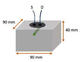
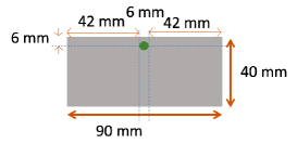
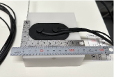
To test the proposed algorithm, the following phantom experiment was performed using TRS-21 (Hamamatsu Photonics K. K., Japan). A solid phantom with an absorber rod (INO, Canada) was prepared and optical fibers for the source and detector were attached with a holder as shown in the left panel of Fig. 1. As shown in the middle panel of Fig. 1, the absorber rod of diameter was embedded below the surface of the phantom. The right panel of Fig. 1 shows a photo of the actual experiment setup.
The optical properties of the phantom were , , and ( is the refractive index of the phantom). The absorber rod shares the same and but (This means ).
Given that the absorber rod penetrated the phantom in one direction (from front to back), the holder was moved in another direction (from left to right, perpendicular to the rod) with a pitch . That is, time-resolved photon counts were taken three times at one position and the holder was moved to the right. At each position, the average of three measurements was taken. There were nine measurement points (): , , , , , , , , and both for the SD distance and ().
At each point (), arrived photons are scored every with . To obtain , we took the moving average for every temporal profile by taking five points before and after each time (average of 11 temporal points). Here, is the reflectance which corresponds to .
Figure 1. The phantom. (Left) Schematic figure of the phantom experiment. (Middle) A cross section of the phantom. (Right) The experimental setup.
In each temporal profile, we considered the time period during for which the peak of the temporal profile lies. We set , . Indeed, the peak of the source is approximately at . Define
where are reflectances for the th SD (source-detector) pair. With unknown positive constants , we can write
The constants depend on experimental conditions and in many cases take different values for different . We have
Let us define
where is a constant. We set . Then we have
where
We will reconstruct from the data using the series for .
2.3. Recursive algorithm for the inverse series
We assume that is independent of and write . The light emitted at is detected at . For spatial variables and time , discretization is done as follows:
where is the temporal resolution of measurements, , and
In our optical tomography, , , or . Moreover, , .
Let us define vectors , , , as
and
For , we define , as
and
We set
where and . We introduce as
for . We note that
Let us define matrix as
Then we can write
Let be a regularized pseudoinverse of .
Let us define vector as
By taking the time difference, we obtain
We have
where for each ,
for , . The matrix is introduced similarly:
for , . Then we can write
Let be a regularized pseudoinverse of . We write
where
To solve the inverse problem, we introduce
for vectors . The inverse series for the forward series can be recursively constructed as follows. Let us introduce vectors which have a recursive structure:
for . We note that the number of compositions for is .
Let us express the th-order Rytov approximation as
where
Then the reconstructed absorption coefficient is written as
where .
3. Results
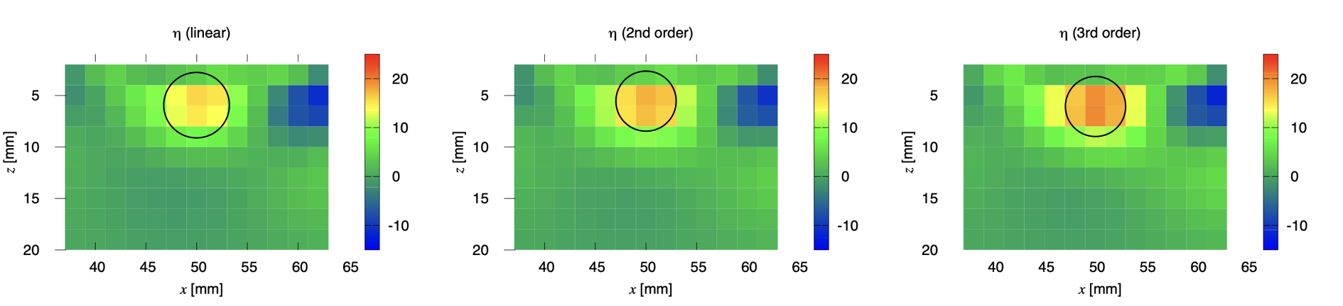
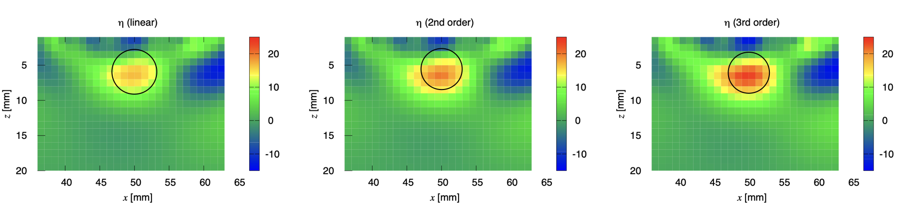
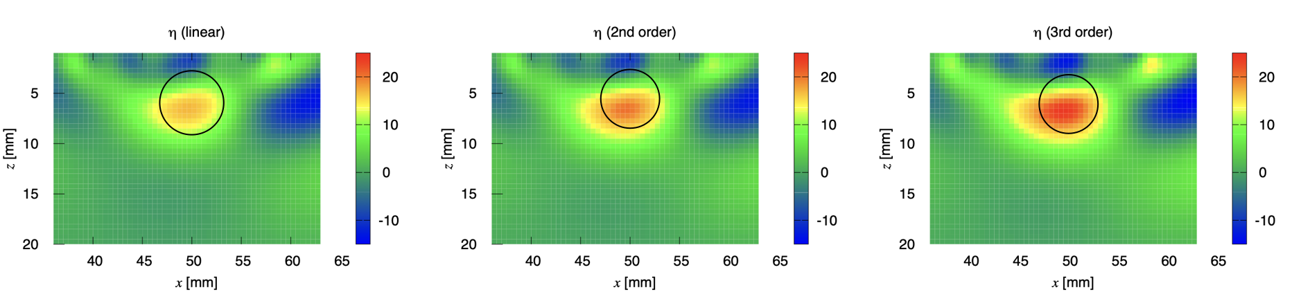
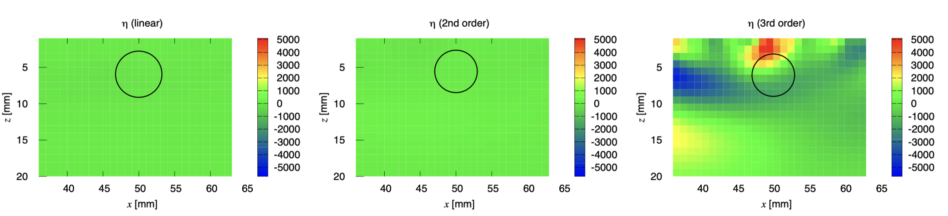
Reconstructed images are shown in Figs. 2 through 5. In each figure, the left panel shows the linear reconstruction (), i.e., the conventional Rytov approximation, the center panel shows the reconstruction for , and the right panel is the reconstructed image when . The black circle in each panel shows the true position of the absorber rod. In all cases, largest singular values were used. The SD distance was for Figs. 2, 3, and 4. In Fig. 5, . For the resolution, in Fig. 2, in Fig. 3, in Fig. 4, and for Fig. 5.
Figure 2. In the case of and . Reconstructed images, from the left, (the conventional Rytov approximation), , and . The true position of the absorber rod is shown by a black circle.
Figure 3. In the case of and . Reconstructed images, from the left, (the conventional Rytov approximation), , and . The true position of the absorber rod is shown by a black circle.Figure 4. In the case of and . Reconstructed images, from the left, (the conventional Rytov approximation), , and . The true position of the absorber rod is shown by a black circle.Figure 5. In the case of and . Reconstructed images, from the left, (the conventional Rytov approximation), , and . The true position of the absorber rod is shown by a black circle.
4. Discussion
Since the ratio of the absorption coefficients inside and outside the absorber rod is large ( and ) and , the inverse series does not converge and the reconstruction of the value of is difficult. However, Figs. 2, 3, and 4 show that the target is more clearly reconstructed if nonlinear terms are added.
We found in [31] that the depth of the center of the banana is , where is the distance between the source and detector. According to this formula, the depth of the banana is . When the SD distance , the depth of the banana is , which is deeper than the depth of the absorber rod. Hence the reconstruction in Fig. 5 was not successful.
In this paper, it was assumed a priori that the absorber rod penetrated the phantom. Three dimensional reconstruction is necessary unless this fact is used. In this case, the formulation developed in this paper can be extended in a straightforward manner.
We note that in many cases diffuse optical tomography in time domain can be formulated using the time-independent diffusion equation by the Laplace or Fourier transform. In this case, the reconstruction can be done using the inverse Rytov series in [30], which was developed for the time-independent diffusion equation.
5. Conclusion
In [30], the inverse Rytov series was first constructed for the time-independent diffusion equation. In this paper, we have developed the inverse Rytov series in time domain. To handle experimental time-resolved data, we considered the forward series by the subtraction of the Rytov series. Then the corresponding inverse series could be computed recursively. We used nonlinear Rytov approximations which are proposed in this paper to obtain reconstructed images for the phantom experiment. By this, the use of the inverse Rytov series was demonstrated.
Funding
This work was supported by JST, PRESTO Grant Number JPMJPR2027.
Disclosures
The authors declare that there are no conflicts of interest related to this article.
Data availability
Data underlying the results presented in this paper are not publicly available at this time but may be obtained from the authors upon reasonable request.
References
[1]
D. A. Boas, D. H. Brooks, E. L. Miller, C. A. DiMarzio, M. Kilmer, R. J. Gaudette, and Q. Zhang,
“Imaging the body with diffuse optical tomography,”
IEEE Signal Processing Magazine 18, 57–75 (2001).
[2]
S. R. Arridge,
“Optical tomography in medical imaging,”
Inverse Problems 15, R41–R93 (1999).
[3]
R. Choe, A. Corlu, K. Lee, T. Durduran, S. D. Konecky, M. Grosicka-Koptyra,
S. R. Arridge, B. J. Czerniecki, D. L. Fraker, A. DeMichele, B. Chance, M. A. Rosen, and A. G. Yodh,
“Diffuse optical tomography of breast cancer during neoadjuvant chemotherapy: A case study with comparison to MRI,”
Medical Physics 32, 1128–1139 (2005).
[4]
A. T. Eggebrecht, S. L. Ferradal, A. Robichaux-Viehoever, M. S. Hassanpour, H Dehghani, A. Z. Snyder, T. Hershey, and J. P. Culver,
“Mapping distributed brain function and networks with diffuse optical tomography”
Nature Photonics 8, 448-454 (2005).
[5]
S. R. Arridge,
Methods for the inverse problem in optical tomography
In: Sebbah, P. (eds) Waves and Imaging through Complex Media
(Springer, Dordrecht, 2001).
[6]
S. Moskow and J. C. Schotland,
“Inverse Born series” (Chap. 12 in The Radon Transform;
edited by Ramlau R and Scherzer O)
Volume 22 in the series
Radon Series on Computational and Applied Mathematics
(De Gruyter, 2019)
[7]
G. A. Tsihrintzis and A. J. Devaney,
“Higher-order (nonlinear) diffraction tomography: Reconstruction algorithms and computer simulation,”
IEEE Trans. Imag. Proc. 9, 1560–1572 (2000).
[8]
V. Markel, J. O’Sullivan, and J. C. Schotland,
“Inverse problem in optical diffusion tomography. IV nonlinear inversion formulas,”
J. Opt. Soc. Am. A 20, 903–912 (2003).
[9]
V. Markel and J. C. Schotland,
“On the convergence of the Born series in optical tomography with diffuse light,”
Inverse Problems 23, 1445–1465 (2007).
[10]
G. Y. Panasyuk, V. A. Markel, P. S. Carney, and J. C. Schotland,
“Nonlinear inverse scattering and three-dimensional near-field optical imaging,”
Appl. Phys. Lett. 89, 221116 (2006).
[11]
S. Moskow and J. C. Schotland,
“Convergence and stability of the inverse scattering series for diffuse waves,”
Inverse Problems 24, 065005 (2008).
[12]
S. Moskow and J. C. Schotland,
“Numerical studies of the inverse Born series for diffuse waves,”
Inverse Problems 25, 095007 (2009).
[13]
S. Arridge, S. Moskow, and J. C. Schotland,
“Inverse Born series for the Calderon problem,”
Inverse Problems 28, 035003 (2012).
[14]
K. Kilgore, S. Moskow, J. C. Schotland,
“Inverse Born series for scalar waves,”
J. Comput. Math. 30, 601–614 (2012).
[15]
M. Machida and J. C. Schotland,
“Inverse Born series for the radiative transport equation,”
Inverse Problems 31, 095009 (2015).
[16]
K. Kilgore, S. Moskow, and J. C. Schotland,
“Convergence of the Born and inverse Born series for electromagnetic scattering,”
Applicable Analysis 96, 1737–1748 (2017).
[17]
F. J. Chung, A. C. Gilbert, J. G. Hoskins, and J. C. Schotland,
“Optical tomography on graphs,”
Inverse Problems 33, 055016 (2017).
[18]
H. A. H. Shehadeh, A. E. Malcolm, and J. C. Schotland,
“Inversion of the Bremmer series,”
J. Comput. Math. 35, 586–599 (2017).
[19]
P. Bardsley and F. G. Vasquez,
“Restarted inverse Born series for the Schrödinger problem with discrete internal measurements,”
Inverse Problems 30, 045014 (2014).
[20]
A. Lakhal,
“A direct method for nonlinear ill-posed problems,”
Inverse Problems 34, 025002 (2018).
[21]
A. Abhishek, M. Bonnet, and S. Moskow,
“Modified forward and inverse Born series for the Calderon and diffuse-wave problems,”
Inverse Problems 36, 114001 (2020).
[22]
J. G. Hoskins and J. C. Schotland,
“Analysis of the inverse Born series: an approach through geometric function theory,”
Inverse Problems 38, 074001 (2022).
[23]
V. Markel and J. C. Schotland,
“Reduced inverse Born series: a computational study,”
J. Opt. Soc. Am. A 39, C179–C189 (2022).
[24]
N. DeFilippis, S. Moskow, and J. C. Schotland,
“Born and inverse Born series for scattering problems with Kerr nonlinearities,”
Inverse Problems 39, 125015 (2023).
[25]
S. Mahankali and Y. Yang,
“Norm-dependent convergence and stability of the inverse scattering series for diffuse and scalar waves,”
Inverse Problems 39, 054005 (2023).
[26]
J. B. Keller,
“Accuracy and validity of the Born and Rytov approximations,”
J. Opt. Soc. Am. 59, 1003–1004 (1969).
[27]
E. Kirkinis,
“Renormalization group interpretation of the Born and Rytov approximations,”
J. Opt. Soc. Am. A 25, 2499–2508 (2008).
[28]
G. A. Tsihrintzis and A. J. Devaney,
“Higher order (nonlinear) diffraction tomography: Inversion of the Rytov series,”
IEEE Trans. Info. Theory 46, 1748–1761 (2000).
[29]
S. Park, M. V. de Hoop, H. Calandra, and C. Shin,
“Full waveform inversion: A diffuse optical tomography point of view,”
SEG Technical Program Expanded Abstracts 30, 2471–2475 (2011).
[30]
M. Machida,
“The inverse Rytov series for diffuse optical tomography,”
Inverse Problems 39, 105012 (2023).
[31]
M. Machida, K. Osada, and K. Kagawa,
preprint (arXiv:2208.07718)