Optimal Kernel Orchestration for Tensor Programs with Korch

Abstract.

Kernel orchestration is the task of mapping the computation defined in different operators of a deep neural network (DNN) to the execution of GPU kernels on modern hardware platforms. Prior approaches optimize kernel orchestration by greedily applying operator fusion, which fuses the computation of multiple operators into a single kernel, and miss a variety of optimization opportunities in kernel orchestration.

This paper presents Korch, a tensor program optimizer that discovers optimal kernel orchestration strategies for tensor programs. Instead of directly fusing operators, Korch first applies operator fission to decompose tensor operators into a small set of basic tensor algebra primitives. This decomposition enables a diversity of fine-grained, inter-operator optimizations. Next, Korch optimizes kernel orchestration by formalizing it as a constrained optimization problem, leveraging an off-the-shelf binary linear programming solver to discover an optimal orchestration strategy, and generating an executable that can be directly deployed on modern GPU platforms. Evaluation on a variety of DNNs shows that Korch outperforms existing tensor program optimizers by up to 1.7$\times$ on V100 GPUs and up to 1.6$\times$ on A100 GPUs. Korch is publicly available at https://github.com/humuyan/Korch.

1. Introduction

Enabling high-performance execution of deep neural networks (DNNs) is critical in many ML applications, including autonomous driving (heisley1991autodriving, ), object detection (papageorgiou2000trainable, ), machine translation (bert, ), and content generation (song2020score, ). A key bottleneck is the mapping of a DNN’s high-level representation to the corresponding hardware-specific computation that can be dispatched to accelerators. A DNN model is represented as a directed acyclic graph (DAG), where each node is a tensor operator (e.g., matrix multiplication or convolution) and each edge represents a tensor (i.e., an $n$-dimensional array) shared between operators. On the other hand, computation on modern hardware accelerators (e.g., GPUs and TPUs) is organized in kernels, each of which is a function simultaneously executed by multiple hardware threads in a single-program-multiple-data (SPMD) fashion (darema1988spmd, ).

To map operators defined in a DNN model to kernels, existing deep learning frameworks (tvm, ; abadi2016tensorflow, ; tensorrt, ; pytorch, ) apply operator fusion, a common form of optimization that fuses the computation of multiple tensor operators into a single kernel to reduce kernel launch overhead and eliminate unnecessary instantiation of intermediate results. For example, TensorFlow (abadi2016tensorflow, ), TensorRT (tensorrt, ), and TVM (tvm, ) consider operator fusion rules manually designed by domain experts and greedily apply these fusion rules whenever possible. DNNFusion (dnnfusion, ) classifies operators into five types based on the data dependencies between the input and output elements of each operator, which allows DNNFusion to develop rules for specific combinations of types instead of combinations of operators. Although existing rule-based operator fusion approaches improve the performance of DNNs on modern accelerators, they have two key limitations.

First, kernel fusion at the operator level is too coarse-grained to unlock all potential optimizations, as some operators achieve suboptimal performance when running in a single kernel. A potential class of optimizations is to decompose these operators into fine-grained components, and fuse components with identical parallelism degrees and memory access patterns across operators into a single kernel. However, these optimizations are excluded in existing frameworks since they cannot be directly represented as operator fusions. One such example is the commonly-used softmax operator, which converts a vector of numbers to a vector of probabilities:

(1) $${\tt softmax}(x_{i})={e^{x_{i}}}/{\sum_{j}e^{x_{j}}}$$

A softmax includes element-wise computation (i.e., the exponential function), vector-wise aggregation (i.e., the summation term in the denominator), and vector-wise broadcast (i.e., the scaling factor $s={1}/{\sum_{j}{e^{x_{j}}}}$ is used to compute all output elements). The three components in softmax involve different degrees of parallelism and memory access patterns, making it challenging to generate a single high-performance kernel for softmax. Meanwhile, generating a dedicated kernel for each of these components in softmax is also suboptimal since this would result in high kernel launch overhead and unnecessary instantiation of intermediate results. We could obtain significant performance improvement by performing inter-operator fusion of the operator’s subcomponents at a finer-grained level (e.g., fusing the element-wise computation of softmax with element-wise components in the previous or next operator).

A second issue with existing operator fusion approaches is their reliance on manually-designed rules to fuse operators greedily, which require significant engineering effort and may miss subtle optimizations that are hard to discover manually. Prior work (jia2019taso, ) has also shown that operation fusion rules designed for one type of device do not directly apply to other device types (e.g., a different generation of GPUs), which is problematic as an increasingly diverse set of AI accelerators have been introduced to deploy DNN computation.

In this paper, we first identify kernel orchestration, the task of orchestrating the computation defined in different operators of a DNN model to the execution of kernels on modern hardware accelerators. This task has been mostly ignored by prior approaches, resulting in missed optimization opportunities. To this end, we introduce Korch, an automated and systematic approach to discovering optimal kernel orchestration strategies for tensor programs. Different from existing deep learning frameworks, which use rule-based strategies to fuse operators into kernels, Korch first applies operator fission to decompose each tensor operator into a small set of basic tensor algebra primitives. Computation defined in each tensor primitive involves the same parallelism degree and data access pattern, making it efficient to execute a tensor primitive in a single kernel. Therefore, primitive graphs provide a more flexible representation for organizing computation of a DNN model compared to the commonly used computation graphs.

Second, to map a primitive graph to kernels, Korch uses a depth-first search algorithm to identify all possible kernels for a primitive graph. Korch formulates kernel orchestration as a constrained optimization problem and uses an off-the-shelf binary linear programming solver to discover an optimal strategy to map tensor algebra primitives into kernels while minimizing execution cost. Finally, Korch uses the strategy identified by the solver to construct kernels and generate an executable that can be directly deployed on modern GPU platforms.

We evaluate Korch on both standard DNN benchmarks as well as emerging workloads and compare Korch with existing tensor program optimizers. Experimental results show that Korch outperforms existing frameworks by up to 1.7$\times$ and 1.6$\times$ on NVIDIA V100 and A100 GPUs, respectively. For most DNNs in our evaluation, the best kernel execution strategy discovered by Korch is outside of the search space of existing operator fusion strategies.

This paper makes the following contributions:

• We identify the kernel orchestration task and unlock a variety of previously missing kernel optimizations.

• We introduce operator fission to decompose operators into fine-grained primitives to enable cross-operator fusion for maximizing kernel efficiency.

• We develop a binary linear programming algorithm to optimally map primitive graphs to kernels.

• We implement Korch and thoroughly evaluate it, showing up to 1.7$\times$ improvement over existing approaches.

2. Overview

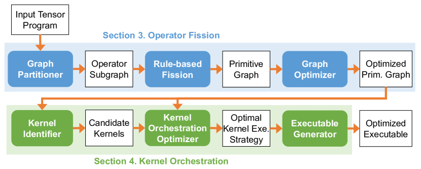
Figure 1. An overview of Korch.

Figure 1 shows an overview of Korch. The input to Korch is a tensor program to be optimized, which is represented as a computation graph whose nodes and edges are tensor algebra operators and data dependencies between them, respectively. Similar to prior work (wang2021pet, ; MetaFlow, ), Korch first partitions an input computation graph into smaller subgraphs to reduce the optimization space associated with each subgraph while preserving optimization opportunities.

For each subgraph, Korch’s operator fission engine uses a rule-based approach to decoupling each operator into one or multiple tensor algebra primitives and generating a primitive graph, which is functionally equivalent to the original computation graph. Korch’s primitive graph optimizer adopts the superoptimization techniques introduced in prior work (jia2019taso, ) and optimizes a primitive graph by using the graph transformations discovered by TASO (jia2019taso, ). By decoupling tensor operators into fine-grained primitives, Korch enables additional primitive-graph-level optimizations that are infeasible to be performed at the operator graph level (see Section 3). This decomposition also allows Korch to perform more flexible kernel orchestration by directly choosing subgraphs of the primitive graph as candidate kernels (see Section 4).

To map tensor algebra primitives to GPU kernels, Korch’s kernel identifier uses a depth-first search algorithm to identify all possible kernels for a given primitive graph. Korch’s kernel profiler then measures the runtime performance of each candidate kernel. Korch formulates kernel orchestration as a binary linear programming (BLP) problem and uses an off-the-shelf BLP solver to discover an optimal kernel orchestration strategy. In particular, Korch’s kernel orchestration optimizer takes all identified kernels and their execution latencies as input and employs a BLP solver to select an optimal strategy, which executes a subset of the candidate kernels and computes the output of the tensor program based on the inputs while minimizing total execution cost. Finally, the optimal execution strategy is used by Korch’s executable generator to produce an executable for the input tensor program. We describe the operator fission and kernel orchestration components in Section 3 and Section 4 respectively.

3. Operator Fission

(a)

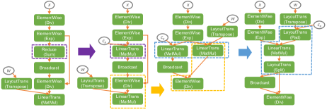
(b)

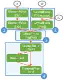
(c)

Figure 2. Operator fission enables subsequent optimizing transformations on primitive graphs. In Figure 2(b), the dotted boxes in the same color indicate a transformation on the primitive graph. The combination of the three transformations fuses the reduce primitive in Softmax and the subsequent MatMul into a single MatMul.

Existing deep learning frameworks optimize kernel orchestration by applying operator fusion to opportunistically fuse multiple tensor operators into a single GPU kernel (tvm, ; tvm_auto_tuner, ). However, directly applying fusion at the operator level misses a variety of fine-grained, inter-operator optimizations. This is because tensor operators are designed based on their algebraic semantics and properties instead of their implementations on GPUs. As a result, for operators with sophisticated mathematical semantics such as normalization and aggregation, performing all computation defined in such an operator within one kernel results in suboptimal performance.

Based on the above observation, Korch first applies operator fission to decouple each tensor operator into a small set of tensor algebra primitives, each of which carries basic algebraic calculation that involves a unified degree of parallelism and data access pattern. The primitives considered by Korch are divided into four categories based on the relationship between the input and output elements of each primitive.

For each primitive $p$, let $O_{p}(I)$ denote the output tensor of running $p$ on $n$ input tensors $I=(I_{1},...,I_{n})$. For an $m$-dimensional tensor $O$, let $O[\vec{x}]$ denote the output value at position $\vec{x}=(x_{1},...,x_{m})$. Similarly, let $I_{k}[\vec{x}]$ denote the input value at position $\vec{x}$ of the $k$-th input tensor $I_{k}$. We use the above notations to introduce the four categories of tensor algebra primitives considered by Korch.

Elementwise primitives.

For an elementwise primitive $p$, the output tensor shares the same shape and data layout as all input tensors, and the computation for each output element depends on the input elements at the same position:

$$O[\vec{x}]=f(I_{1}[\vec{x}],I_{2}[\vec{x}],...,I_{n}[\vec{x}])$$

Elementwise primitives do not involve layout transformations and can generally be fused with other primitives as a pre- or post-processing step.

Reduce and broadcast primitives.

A reduce primitive takes as input a single tensor and calculates the aggregated result of each row of the input tensor along a given dimension:

$$O[x_{1},...,x_{k-1},x_{k+1},...,x_{m}]$$

$$\quad\quad\quad\quad\quad\quad=\oplus_{x_{k}}I_{1}[x_{1},...,x_{k-1},x_{k},x_{k+1},...,x_{m}],$$

which aggregates along the $k$-th dimension of $I_{1}$, and $\oplus$ is the aggregator. A broadcast primitive performs the reverse, taking a single input tensor and replicating the input tensor along a given dimension:

$$O[x_{1},...,x_{k-1},x_{k},x_{k+1},...,x_{m}]$$

$$\quad\quad\quad\quad\quad\quad=I_{1}[x_{1},...,x_{k-1},x_{k+1},...,x_{m}].$$

Layout transformation primitives.

A layout transformation primitive takes a single tensor as input and transforms its data layout without performing arithmetic operations:

$$O[\vec{x}]=I_{1}[L(\vec{x})],$$

where $\vec{u}=L(\vec{x})$ is a one-to-one mapping from position $\vec{x}$ of the output tensor to position $\vec{u}$ of the input tensor. Note that a layout transformation primitive can have multiple input/output tensors. For example, concatenation and split are considered layout transformation primitives, since they require changing the underlying layouts of the input tensors.

Linear transformation primitives.

Finally, Korch uses linear transformation primitives to capture the compute-intensive operators in DNNs such as matrix multiplication and convolution. Specifically, a primitive $p$ is considered as a linear transformation primitive if its output is linear to all input tensors:

$$\forall Y,Z,\vec{x},1\leq k\leq n.\quad O(I_{1},...,I_{k-1},Y+Z,...)[\vec{x}]$$

$$=O(I_{1},...,I_{k-1},Y,...)[\vec{x}]+O(I_{1},...,I_{k-1},Z,...)[\vec{x}],$$

$$\alpha\cdot O(I_{1},...,I_{k-1},Y,...)[\vec{x}]=O(I_{1},...,I_{k-1},\alpha\cdot Y,...)[\vec{x}]$$

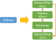
Figure 3. The operator fission rule for Softmax.

Table 1. Examples of some frequently used primitves.

Primitive Type	Representative Operators
Elementwise	Add, Sub, Mul, Div, Relu, Sqrt, Erf
Reduce and broadcast	ReduceSum, ReduceMean, MaxPool, Broadcast
Layout transformation	Transpose, Split, Concat, Slice, Pad, Reshape
Linear transformation	Conv, GEMM, Batched GEMM

Table 1 shows representative operators for the four types of primitives. For each DNN operator, Korch requires developers to specify an operator fission rule, which is used to decouple the DNN operator into the specified primitives. Each operator fission rule is a transformation from a DNN operator to a functionally equivalent primitive graph. To demonstrate the complexity of designing an operator fission rule, Figure 3 shows the operator fission rule for softmax (see Equation 1), which is decomposed into an elementwise exponential, a reduce, a broadcast, and an elementwise division primitive.

Operator fission enables two important classes of optimizations missing in existing deep learning frameworks. First, by decoupling operators into fine-grained primitives, operator fission enables optimizing transformations on primitive graphs; these transformations are impossible to apply at the operator level. Figure 2(b) shows such an example to optimize multi-head attention in Transformer (vaswani2017attention, ). First, the reduce primitive of Softmax is substituted by a linear transformation primitive (i.e., MatMul) by introducing a constant input tensor $C_{s}$ whose elements are all ones. Second, the elementwise division primitive of Softmax is swapped with the subsequent MatMul by applying a transformation discovered by prior work (jia2019taso, ). Finally, the two MatMuls with a shared input are fused by introducing a Pad and a Split primitive. These transformations allow Korch to fuse the reduce primitive in Softmax with a MatMul.

A second advantage of operator fission is enabling more flexible kernel orchastration. Specifically, for the optimized primitive graph in Figure 2(c), Korch maps Div and Exp into kernel ①, which achieves the same performance as just performing Div in a single kernel due to the low arithmetic intensity of elementwise computation. Similarly, Transpose and Pad are mapped to kernel ②, which has the same performance as a single Transpose kernel. MatMul itself is mapped to kernel ③, since it is compute-intensive and mapping it as a single kernel allows Korch to use kernels provided by CUDA libraries (see details in Section 5.2). Finally, the Split, Broadcast, and Div primitives are all mapped to kernel ④. Both Split and Broadcast do not introduce arithmetic operations and are cheap to execute. The performance improvement of this optimization is due to the fact that kernel ④ is much faster than launching a Softmax kernel.

Supporting new operators.

The four categories of primitives listed above are sufficient to represent a variety of tensor operators used in today’s DNNs, including all DNN benchmarks in our evaluation. However, there are tensor operators that cannot be represented using the above primitives. One such operator is Topk, which returns the $k$ largest elements of an input tensor along a given dimension. For such operators, Korch treats them as opaque primitives and will only optimize the rest of the primitive graph in graph optimizations.

4. Kernel Orchestration

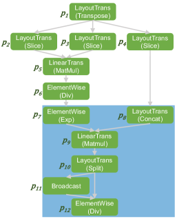
(a)

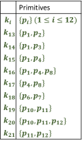
(b)

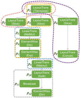
(c)

Figure 4. An example of kernel orchestration for a subgraph of self attention (vaswani2017attention, ). The shadowed subgraph in Figure 4(a) is similar with the primitive graph transformation result in Figure 2.

This section describes Korch’s kernel orchestration engine, which takes a primitive graph as an input and discovers an optimal strategy to map the primitives to kernels while minimizing execution latency. A primitive graph is represented as a directed acyclic graph $\mathcal{G}=(\mathcal{P},\mathcal{E})$, where each node $p\in\mathcal{P}$ is a tensor algebra primitive, and each edge $(p_{1},p_{2})\in\mathcal{E}$ denotes a tensor that is an output of $p_{1}$ and an input of $p_{2}$. Computations on GPUs are organized as kernels, each of which is a function simultaneously executed by multiple threads in a single-program-multiple-data (SPMD) fashion. Each kernel executes one or multiple primitives. To avoid circular dependencies between kernels (i.e., two kernels depend on each other to start), the primitives included in a kernel must form a convex subgraph of $\mathcal{G}$.

Definition 0 (Convex subgraph).

For a primitive graph $\mathcal{G}=(\mathcal{P},\mathcal{E})$, a set of nodes $\mathcal{P}^{\prime}\subseteq\mathcal{P}$ forms a convex subgraph of $\mathcal{G}$ if and only if there do not exist nodes $p_{1},p_{2}\in\mathcal{P}^{\prime}$ and another node $q\in\mathcal{P}\setminus\mathcal{P}^{\prime}$ such that $p_{1}\overset{\mathcal{G}}{\leadsto}q$ and $q\overset{\mathcal{G}}{\leadsto}p_{2}$, where $x\overset{\mathcal{G}}{\leadsto}y$ indicates that there exists a path from $x$ to $y$ in $\mathcal{G}$.

For the primitive graph in Figure 4(a), node set $\{p_{1},p_{4},p_{8}\}$ forms a convex subgraph of $\mathcal{G}$ and thus can be executed in a single kernel. On the other hand, we cannot execute node set $\{p_{1},p_{2},p_{5}\}$ (a non-convex subgraph of $\mathcal{G}$) in a single kernel, since it has a circular dependency with the kernel that executes $p_{3}$ (i.e., $p_{5}$ depends on $p_{3}$ which depends on $p_{1}$). Korch uses execution states to identify all convex subgraphs of a given primitive graph.

Definition 0 (Execution state).

A set of nodes $\mathcal{P}^{\prime}\subseteq\mathcal{P}$ is an execution state of a primitive graph $\mathcal{G}=(\mathcal{P},\mathcal{E})$ if for any edge $(p_{1},p_{2})\in\mathcal{E}$, $p_{2}\in\mathcal{P}^{\prime}$ implies $p_{1}\in\mathcal{P}^{\prime}$.

Transiting from an execution state to another allows Korch to identify all possible convex subgraphs, as shown in Theorem 3. The computation of each convex subgraph of $\mathcal{G}$ can be performed in a candidate kernel.

Theorem 3.

A set of nodes $\mathcal{P}^{\prime}\subseteq\mathcal{P}$ forms a convex subgraph of $\mathcal{G}=(\mathcal{P},\mathcal{E})$ if and only if $\mathcal{P}^{\prime}$ is the difference of two execution states $\mathcal{P}_{1}$ and $\mathcal{P}_{2}$: $\mathcal{P}^{\prime}=\mathcal{P}_{1}\setminus\mathcal{P}_{2}$.

Proof.

If $\mathcal{P}^{\prime}=\mathcal{P}_{1}\setminus\mathcal{P}_{2}$, the following will show that $\mathcal{P}^{\prime}$ is a convex subgraph. Suppose there exist $p_{1},p_{2}\in\mathcal{P}^{\prime}$ and $q\in\mathcal{P}\setminus\mathcal{P}^{\prime}$ such that $p_{1}\overset{\mathcal{G}}{\leadsto}q$ and $q\overset{\mathcal{G}}{\leadsto}p_{2}$. Therefore, $p_{1},p_{2}\in\mathcal{P}_{1}$ and $p_{1},p_{2}\notin\mathcal{P}_{2}$. Also we can get $q\notin\mathcal{P}_{1}$ or $q\in\mathcal{P}_{2}$. If $q\notin\mathcal{P}_{1}$, $q\overset{\mathcal{G}}{\leadsto}p_{2}$ and $p_{2}\in\mathcal{P}_{1}$ will contradict that $\mathcal{P}_{1}$ is an execution state. If $q\in\mathcal{P}_{2}$, $p_{1}\overset{\mathcal{G}}{\leadsto}q$ and $p_{1}\notin\mathcal{P}_{2}$ will contradict that $\mathcal{P}_{2}$ is an execution state. In conclusion, the supposition is wrong, so $\mathcal{P}^{\prime}$ is a convex subgraph.

If $\mathcal{P}^{\prime}$ is convex graph, let $\mathcal{S}=\{p\mid p\notin\mathcal{P}^{\prime}\text{ and }\exists(p,p^{\prime})\in\mathcal{E},p^{\prime}\in\mathcal{P}^{\prime}\}$. Then we can construct two execution states $\mathcal{P}_{1}=\{p\mid p\in\mathcal{P}^{\prime}\text{ or }\exists p^{\prime}\in\mathcal{P}_{1},(p,p^{\prime})\in\mathcal{E}\}$ and $\mathcal{P}_{2}=\{p\mid p\in\mathcal{S}\text{ or }\exists p^{\prime}\in\mathcal{P}_{2},(p,p^{\prime})\in\mathcal{E}\}$. From the convexity of $\mathcal{P}^{\prime}$ we can get $\mathcal{P}^{\prime}=\mathcal{P}_{1}\setminus\mathcal{P}_{2}$. ∎

Intuitively, the number of execution states increases linearly with the depth (i.e., the number of operators on the critical path) and exponential with the width (i.e., the number of concurrent operators) of a primitive graph. While the number of execution states for a primitive graph can increase exponentially with the number of primitives, we observe that modern DNN architectures are generally deep instead of wide, resulting in a limited number of execution states and making it tractable to explicitly consider all execution states. For a primitive graph, we expect approximately $O(|\mathcal{P}|)$ execution states and $O(|\mathcal{P}|^{2})$ candidate kernels for simplicity, where $|\mathcal{P}|$ is the number of primitives in the graph. Such simplification has also been adopted in prior work (tarnawski2021piper, ).

Next, we describe Korch’s kernel identifier, which uses a depth-first search algorithm for identifying all valid kernels in a primitive graph.

Algorithm 1 Depth-first-search to identify kernels. Profiling takes a set of primitives as an input, generates a kernel for the defined tensor algebra computation, and profiles the runtime performance of the kernel. Profiling returns $\infty$ if such a kernel cannot be generated. We describe the kernel profiler in Section 5.2.

1:Input: A primitive graph $\mathcal{G}=(\mathcal{P},\mathcal{E})$

2:Output: All possible kernels of $\mathcal{G}$

3:$\mathcal{B}=\{\}$ $\triangleright$ $\mathcal{B}$ is a database of $\mathcal{G}$’s execution states

4:function Dfs($\mathcal{X}$) $\triangleright$ $\mathcal{X}$ is the current execution state

5:    for $v\in\mathcal{P}\setminus\mathcal{X}$ do $\triangleright$ find a new primitive to execute

6:         if $\forall(u,v)\in\mathcal{E}.u\in\mathcal{X}$ then

7:             $\mathcal{X}^{\prime}=\mathcal{X}\cup\{v\}$

8:             if $\mathcal{X}^{\prime}\notin\mathcal{B}$ then

9:                 $\mathcal{B}=\mathcal{B}\cup\{\mathcal{X}^{\prime}\}$

10:                 Dfs($\mathcal{X}^{\prime}$)                           

11:Dfs($\emptyset$)

12:$\mathcal{K}=\{\}$ $\triangleright$ $\mathcal{K}$ is a database of $\mathcal{G}$’s kernels

13:for $\mathcal{D}_{1}\in\mathcal{B}$ do

14:    for $\mathcal{D}_{2}\in\mathcal{B}$ do

15:         if $\mathcal{D}_{1}\subset\mathcal{D}_{2}$ then

16:             $\mathcal{P}^{\prime}=\mathcal{D}_{2}\setminus\mathcal{D}_{1}$

17:             for $\mathcal{O}\subset\mathcal{P}^{\prime}$ do $\triangleright$ $\mathcal{O}$ is a possible output set of $\mathcal{P}^{\prime}$

18:                 $K,\mbox{\rm\em latency}=\textsc{Profiling}(\mathcal{P}^{\prime},\mathcal{O})$

19:                 if $\mbox{\rm\em latency}\neq\infty$ then

20:                     $\mathcal{K}=\mathcal{K}\cup\{K,\mathcal{P}^{\prime},\mathcal{O},\mbox{\rm\em latency}\}$                                            

21:Return $\mathcal{K}$

4.1. Kernel Identifier

Algorithm 1 shows an algorithm to identify all possible kernels in a primitive graph $\mathcal{G}$. The algorithm starts from an empty execution state $\mathcal{X}=\emptyset$ and uses depth-first search (DFS) to enumerate all possible execution states, which are maintained in a database $\mathcal{B}$. For each pair of execution states $(\mathcal{D}_{1},\mathcal{D}_{2})$, their set difference identifies a set of primitives $\mathcal{P}^{\prime}=\mathcal{D}_{2}\setminus\mathcal{D}_{1}$ that can potentially form a kernel.

Considering a subgraph $\mathcal{G^{\prime}=(P^{\prime},E^{\prime})}$, we now identify the inputs and outputs of $\mathcal{G^{\prime}}$. Obviously, the inputs of $\mathcal{G^{\prime}}$ should be all the nodes of $\mathcal{G^{\prime}}$ with zero in-degree. However, the outputs of $\mathcal{G^{\prime}}$ are not simply all the nodes with zero out-degree, since some nodes with positive out-degree may become the inputs for another candidate kernel subgraph. We define the possible output set of $\mathcal{G^{\prime}}$ as follows:

Definition 0 (Possible output set).

A set $\mathcal{O}$ of nodes is a possible output set of a candidate subgraph $\mathcal{G^{\prime}=(P^{\prime},E^{\prime})}$ if and only if $\forall u\in\mathcal{O}$, $\exists(u,v)\in\mathcal{E}$ such that $v\in\mathcal{P}\setminus\mathcal{P^{\prime}}$.

Both $\mathcal{P}^{\prime}$ and $\mathcal{O}$ are sent to the kernel profiler to generate a kernel for its primitives. If such a kernel can be successfully generated, the kernel profiler also returns the measured execution latency of the kernel; otherwise, the profiler returns infinity to indicate that $\mathcal{P}^{\prime}$ is not supported by Korch’s DNN backends. Section 5.2 introduces Korch’s kernel profiler for generating and profiling kernels for a given set of primitives. For the primitive graph in Figure 4(a), Figure 4(b) shows all valid kernels identified by Korch’s kernel profiler.

4.2. Kernel Orchestration Optimizer

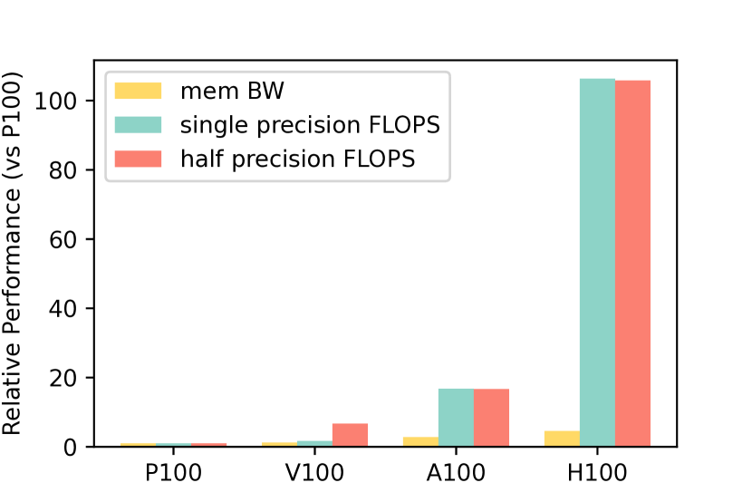
Figure 5. Comparing memory bandwidth and floating-point throughput across GPU generations. The y-axis is normalized to the performance of P100 GPUs.

This section first defines the kernel orchestration problem and then formalizes it as a constrained optimization task. Korch uses a binary integer linear programming algorithm to discover a kernel orchestration strategy that minimizes the total execution cost on GPUs.

Kernel orchestration problem.

For a given primitive graph $\mathcal{G}$, let $K_{1},...,K_{M}$ denote all the kernels discovered by the kernel identifier (see Section 4.1). The kernel orchestration optimizer takes a primitive graph $\mathcal{G}$ and all identified kernels as input and discovers an optimal kernel execution strategy, which is represented by an $M$-dimensional binary vector $\vec{u}=\langle u_{1},...,u_{M}\rangle$, where $u_{i}=1$ if $K_{i}$ is executed in this strategy, and $u_{i}=0$ otherwise. Korch follows prior work (jia2019taso, ) and assumes that the run time of an execution strategy is the summation of individual kernels’ run times:

(2) $$\mbox{\rm\em Cost}(\vec{u})=\sum_{i=1}^{M}c_{i}u_{i},$$

where $c_{i}$ is the measured run time of kernel $K_{i}$.

To discover a kernel execution strategy that minimizes run time, our key idea is to formalize kernel orchestration as a binary linear programming (BLP) task and find an optimal strategy using an off-the-shelf BLP solver, which will be introduced in Section 5. Korch uses two matrices $I$ and $O$ to represent the correlation between kernels and primitives. Specifically, $I$ and $O$ are both binary matrices of size $M\times|\mathcal{P}|$, where $I_{ij}=1$ if and only if primitive $p_{j}$ is an input of kernel $K_{i}$, and $O_{ij}=1$ if and only if primitive $p_{j}$ is an input of kernel $K_{i}$. Therefore, $\sum_{i=1}^{M}O_{ij}u_{i}$ calculates how many times primitive $p_{j}$ is executed. A key difference between Korch and prior work is that existing tensor program optimizers partition computations defined in a DNN architecture into kernels in a disjoint way (i.e., no redundant computation), while Korch allows a primitive to be executed multiple times (i.e., $\sum_{i=1}^{M}O_{ij}u_{i}>1$). This relaxation is based on an important observation that the floating-point throughput of modern GPUs is increasing at a much higher rate than their memory bandwidth, as shown in Figure 5. Therefore, Korch allows primitives to be executed multiple times to opportunistically reduce memory accesses and kernel launch overheads. For example, Figure 4(c) shows an optimal kernel orchestration strategy that executes $p_{1}$ three times to reduce kernel launch and data movement overheads.

Comparison with tensor rematerialization.

Tensor rematerialization is a common technique used in DNN training to reduce memory overhead of DNN training by discarding some intermediate results during forward processing and rematerializing the discarded tensors during backpropagation. Tensor rematerialization reduces the peak memory usage of DNN training at the cost of re-executing some kernels multiple times in a training iteration. Instead of reducing overall accesses to GPU device memory, tensor rematerialization actually increases memory accesses since some kernels are executed multiple times. In contrast, the primitive redundancy in Korch is designed to allow opportunistic fusion of kernels with overlapping primitives.

We now describe our binary linear programming formulation. For a given primitive graph $\mathcal{G}=(\mathcal{P},\mathcal{E})$, let $\mathcal{T}\subseteq\mathcal{P}$ denote the set of output primitives. The BLP task minimizes the objective defined in Equation 2 by considering the following constraints.

Output constraints.

The output constraints guarantee that a valid strategy executes all primitives that are the output of the DNN model:

(3) $$\sum_{i=1}^{M}O_{ij}u_{i}\geq 1\quad\quad\forall p_{j}\in\mathcal{T}.$$

Dependency constraints.

The dependency constraints check data dependencies between different kernels — a kernel can be executed only if all its input tensors have been computed by prior kernels:

(4) $$\sum_{i=1}^{M}O_{ij}u_{i}\geq I_{k,j}u_{k}\quad\quad\forall p_{j}\in\mathcal{P},k\in[1,M]$$

Note that Korch does not require all primitives to be executed, and our formulation implicitly performs pruning optimizations. Korch’s kernel execution strategy can be seen as covering the whole computation graph with candidate kernel subgraphs, only with the constraints of subgraph dependencies.

5. Implementation

This section presents our implementation of Korch, with a specific focus on the design of our operator fission engine and kernel orchestration optimizer.

5.1. Operator Fission

Our implementation represents a primitive graph in the ONNX format (onnx, ), which is widely used and mathematically complete. In particular, ONNX operators (onnx_operators, ) include all primitive types introduced in Section 3. Korch’s operator fission engine takes an ONNX graph as input and performs rule-based operator fission to construct an equivalent primitive graph. The output of the operator fission engine is also in the ONNX format.

5.2. Kernel Orchestration Optimizer

Kernel profiler

Korch’s kernel profiler takes a primitive graph as input, generates a GPU kernel for the input graph, and profiles the runtime performance of the kernel. Korch follows prior work and requires that each primitive graph has exactly one output (tvm, ). As a result, each candidate kernel has an arbitrary number of input tensors and produces one output tensor. For each candidate kernel, the profiler examines whether the subgraph includes any linear transformation primitive. If no linear transformation primitive is found, the profiler identifies the current candidate kernel as memory-intensive and sends the subgraph to TVM’s MetaSchedule for hyper-parameter tuning. Otherwise, the profiler identifies the current candidate kernel as compute-intensive.

MetaScheduler (metascheduler, ) is a probabilistic scheduler DSL developed in TensorIR that unifies the pre-existing approaches (i.e., AutoTVM (tvm_auto_tuner, ) and Ansor (ansor, )). Korch uses MetaScheduler to generate high-performance kernels for a given primitive graph and target hardware. Specifically, Korch lowers an ONNX graph to a TensorIR schedule given pre-defined scheduling rules and leverages the Ansor backend to generate the best performing schedule. The kernel profiler then measures the performance of the generated kernel and returns the measured latency, the lowered scheduler, and generated CUDA code back to the kernel orchestration optimizer. Since memory-intensive kernels have relatively simple schedules, most of them can be tuned within 2 minutes through MetaScheduler.

For compute-intensive operators, Korch follows the heuristics used by prior work (e.g., EinNet (zheng2023einnet, )) and directly lowers these primitive graphs to vendor libraries (e.g., cuDNN and cuBLAS) instead of TVM. This design is based on an observation that compute-intensive operators have more complicated schedules and are difficult to automatically generate a kernel that outperforms vendor-provided implementations within a short tuning time. In the rare case where a compute-intensive primitive graph cannot match the parameters defined in vendor libraries, Korch rejects the candidate. Our implementation uses cuDNN (cudnn, ), cuBLAS (cublas, ) and TensorRT (tensorrt, ) as potential backends for compute-intensive operators.

Korch formalizes kernel orchestration as a binary linear programming (BLP) problem by constructing the constraints identified in Section 4, and solves the BLP using PuLP (mitchell2011pulp, ), a Python linear programming solver. The biggest subgraph in our test cases has 584 execution states and 3078 candidate kernels. PuLP can converge to an optimal solution within 1000 seconds for all primitive graphs in our evaluation.

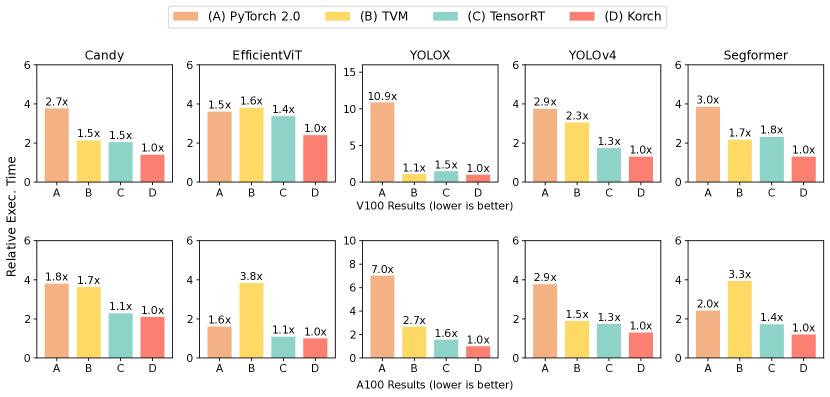
Figure 6. End-to-end performance comparison on V100 and A100.

5.3. Executable Generator

After generating an optimal kernel orchestration strategy and the CUDA code for all selected candidate kernels, Korch stitches the kernels’ implementations together by respecting data dependencies between these kernels. As a result, the end-to-end execution latency of the entire computation graph is consistent with the objective function of the ILP task (i.e., Equation 2). Note that Korch only considers sequential execution of the orchestrated kernels and does not consider inter-kernel optimizations such as CUDA multi-streaming. By modifying the ILP problem formulation, it is possible to take into account more advanced kernel execution strategies, which we leave as future work.

6. Evaluation

6.1. Experimental Setup

Platform

Our evaluation is performed on an Nvidia V100 GPU and an A100 GPU. For the V100, we use an AWSp3.8xlarge instance (p3.2xlarge, ), which is equipped with a 32-core Intel Xeon CPU, four V100 16GB SXM GPUs, CUDA 11.7 and runs Ubuntu 20.04. For the A100, we use the Perlmutter supercomputer, which runs on SUSE Linux Enterprise Server 15 SP4 OS and is equipped with with a 64-core AMD EPYC CPU, four A100 80GB SXM GPUs and CUDA 11.7 on each node.

Workloads

We use five real-world DNNs to evaluate Korch. Candy (johnson2016perceptual, ) is a convolutional neural network (CNN) for fast style transfer. YOLOv4 (bochkovskiy2020yolov4, ) and YOLOX-Nano (ge2021yolox, ) are CNN-based object detectors. Segformer (xie2021segformer, ) is a vision Transformer for semantic segmentation. EfficientViT (cai2022efficientvit, ) is a vision Transformer backbone for high-resolution low-computation vision tasks. For all those workloads, we evaluate with a batch size of one. The input resolutions for Segformer and EfficientViT are 512$\times$512 and 2048$\times$2048, respectively. For other CNNs, we use their default input resolutions: 224$\times$224 for Candy and 416$\times$416 for YOLOs. On V100 GPUs, all DNNs are executed in 32-bit floating points (FP32). On A100 GPUs, we enable tensor cores and execute the DNNs using TF32.

6.2. End-to-end Performance

We first evaluate the end-to-end inference latency on a single GPU, and compare Korch with PyTorch 2.0.1, TVM 0.11 (tvm, ) (commit hash 61a4f21) and TensorRT 8.2 (tensorrt, ).

Figure 6 shows the end-to-end results on V100 and A100. Korch achieves up to 1.7$\times$ speedup on V100 and up to 1.6$\times$ speedup on A100. The average speedups on V100 and A100 are 1.39$\times$ and 1.30$\times$, respectively. Among the five DNN workloads, Segformer and EfficientViT are vision Transformers and heavily optimized by existing DNN frameworks. With the optimal kernel orchestration strategy, Korch can still reduce their latency by up to 1.7$\times$ and 1.4$\times$. For conventional CNNs such as Candy, YOLOv4 and YOLOX-Nano, Korch outperforms existing frameworks by 1.31$\times$ on average. We analyze the optimization improvement and show the new orchestration strategies discovered by Korch in Section 6.3 and Section 6.4.

We observe that Korch achieves a more significant performance improvement on V100 than on A100. As verified by prior approach (zheng2023einnet, ), advanced GPUs like A100 should get more performance benefits theoretically from tensor program optimizations (e.g., kernel fusion), since they offer a higher ratio between computation capability and memory bandwidth (see Figure 5). The reverse behaviors in our experiments can be attributed to two reasons. First, kernel orchestration not only optimizes memory-intensive operators, which are the major source of acceleration from prior kernel fusion approaches, but also improves compute-intensive operators’ performance. We further discuss the difference in Section 6.4 and provide a case study (i.e., Figure 8) to show how Korch considers different data layouts for those compute-intensive operators. Second, Korch’s kernel orchestration relies on TVM for flexible code generation for candidate kernels. Our evaluation also shows that TVM performs worse than highly-optimized TensorRT on A100, indicating that there still remains potential space for improving Korch by leveraging more advanced kernel generation techniques.

6.3. Adaptation Study over TensorRT

In this section, we transplant the implementation of our proposed operator fission to TensorRT to show its effectiveness. Specifically, instead of using the ILP-based kernel orchestration in Figure 2(c), we directly feed the post-operator-fission primitive graph to TensorRT, which then decides the kernel orchestration strategy and uses its own kernels for code generation. Since TensorRT is heavily optimized for the Transformer models, we select Segformer for this study to make the comparison more persuasive. Figure 7 shows the performance comparison on Segformer and we can see that merely applying operator fission leads to a 1.24$\times$ speedup on V100, compared with directly using TensorRT.

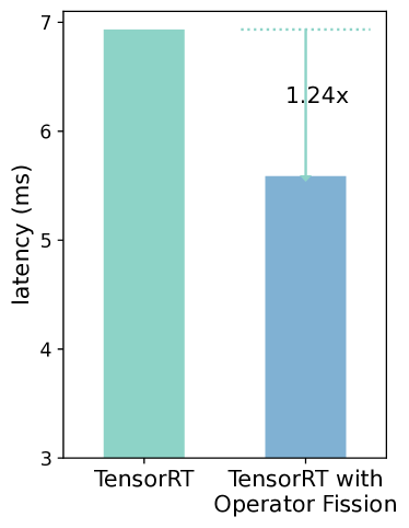
Figure 7. speedup of operator fission: feeding the primitive graph instead of computation graph to TensorRT leads to 1.24x speedup.

6.4. Case Study

To understand how Korch’s optimal kernel orchestration technique enlarges the optimization space, we study some orchestration strategies found by Korch in detail. All results in this section are measured on Nvidia V100 GPU.

Redundant Computing.

Figure 8 compares the kernel orchestration strategy of TensorRT and Korch in the EfficientViT attention block. Korch first applies transformations on the primitive graph to merge ReduceSum and MatMuls, generating the graph from Figure 9 to Figure 8(b). During kernel orchestration, Korch fuses consecutive memory-intensive operators (e.g., $k_{2}$ in Figure 8(b)) and opportunistically fuses Transpose with Matmul to optimize data layout (e.g., comparing $k_{8}$ in Figure 8(a) and $k_{5}$ in Figure 8(b)), which is not considered by TensorRT. In particular, the input matrix to $k_{8}$ in Figure 8(a) has an extreme aspect ratio of 1024:1. After changing the data layout, $k_{5}$ in Figure 8(b) is 3.52x faster than $k_{8}$ in Figure 8(a), with the same TensorRT MatrixMultiply backend. Moreover, Korch allows the Reshape+Transpose+Reshape operators to be executed multiple times in three kernels (i.e., $k_{2}$, $k_{3}$, and $k_{4}$ in Figure 8(b)). Since all these operators are memory-intensive, their latency is mainly determined by the memory I/O overhead. Korch’s mapping strategy reduces the total number of kernels and therefore improves the overall latency. Korch only uses 7 kernels for the EfficientViT attention block, which saves 5 kernels and achieves 3.29$\times$ speedup over TensorRT for the entire subgraph, as shown in Figure 10. If we directly apply kernel orchestration in Figure 8(a)’s graph without primitive graph transformations, the optimizer also needs to do redundant computation (i.e., moving Transpose in $k_{6}$ into $k_{8}$ and $k_{9}$) to optimize the data layout of MatMul in $k_{8}$. However, redundant computing is not considered in prior work, so this data layout transformation is out of the optimization space of prior work.

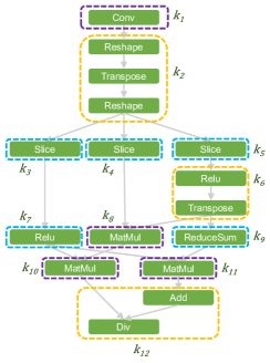
(a)

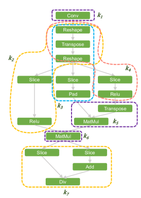
(b)

Figure 8. Comparison of kernel orchestration strategy on an EfficientViT attention block. Before kernel orchestration, Korch first applies graph transformation in Figure 9.

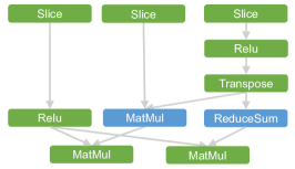
(a)

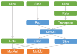
(b)

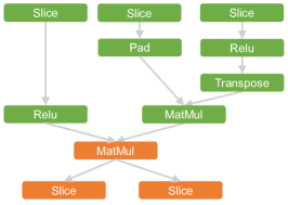
(c)

Figure 9. Primitive graph transformation from Figure 8(a) to Figure 8(b). Nodes with same color indicate a transformation on the primitive graph. Merging of ReduceSum and MatMul is done similarly with Figure 2.

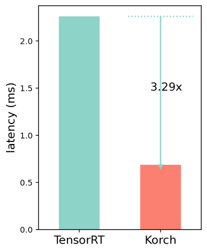
Figure 10. Case study of EfficientViT attention block: Korch’s strategy (Figure 8(b)) achieves 3.29x speedup over TensorRT’s strategy (Figure 8(a)).

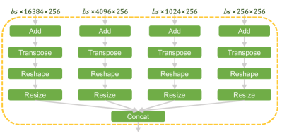
(a)

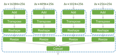
(b)

Figure 11. Two different kernel orchestration strategy on a Segformer subgraph. TVM will always choose strategy (a), but Korch will choose strategy (a) with batch size 1 and strategy (b) with batch size 16.

Map one operator to different kernels.

To optimize Segformer, Korch uses the transformations demonstrated in Figure 2(b) to decompose Softmax, and then applies similar kernel mapping as shown in Figure 4(c). With this strategy, Korch maps Softmax to all four kernels in Figure 2(b) and outperforms TensorRT by 1.50$\times$ for this self-attention block. Moreover, to optimize CNNs such as Candy, Korch can break the boundary of operators during fusion. Figure 12(a) shows a common network pattern in Candy. As can be seen in Figure 12, TensorRT maps InstanceNorm, ReLU and Pad to individual kernels, but Korch can decompose InstanceNorm and fuse part of it into the subsequent ReLU and Pad operators, achieving 1.32$\times$ speedup for this graph pattern.

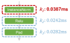
(a)

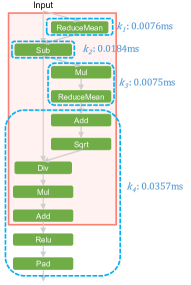
(b)

Figure 12. Comparison of kernel orchestration strategy and kernel latency on a common subgraph pattern in Candy. The red frame in Figure 12(b) is the opeartor fission of InstanceNorm. Korch outperforms TensorRT by 1.32x on this subgraph.

Greedy fusion can be suboptimal.

Figure 11 shows two different kernel orchestration strategies for a subgraph of Segformer. Since all operators are memory-intensive and fusable, TVM directly fuses the entire subgraph into one kernel. However, as shown in Figure 13, fusing the entire graph is efficient with a batch size of 1 but suboptimal with a batch size of 16, since TVM cannot generate a highly optimized kernel for the entire graph. Without modifying the TVM code generation backend, using multiple kernels (Figure 11(b)) to execute this graph leads to 2.24$\times$ speedup.

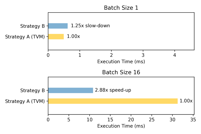
Figure 13. Comparison of different kernel orchestration strategies on a Segformer subgraph. TVM will always choose strategy A, but Korch will choose strategy A for batch size 1 and strategy B for batch size 16.

6.5. Tuning Time

Table 2 shows the number of primitive graph nodes, candidate kernels, and overall tuning time on Perlmutter for all DNNs in our evaluation. Theoretically the number of candidate kernels should be quadratic with the number of nodes, but we observe that the actual number of candidate kernels is far smaller than that. In our implementation, most of the candidate kernels can be rejected with simple heuristics, such as too many operators to generate within one kernel or including multiple linear transformation primitives.

Most of Korch’s tuning time is consumed by TVM’s MetaScheduler for memory-intensive kernels. We utilize the TVM database to avoid tuning the same candidate kernel multiple times. Besides, the tuning of candidate kernels can be parallelized across multiple GPUs. The longest tuning time is 12.2 hours, in which case a single kernel takes 12 hours to tune by the TVM MetaScheduler. Given that kernel tuning is one-time cost, Korch’s tuning overhead is acceptable in real world applications.

Table 2. Number of primitive graph nodes, candidate kernels and end-to-end tuning time on Perlmutter for all the evaluated models.

Model	# Nodes	# Candidate Kernels	Tuning Time
Candy	184	1031	5.5h
EfficientViT	380	2174	11.5h
YOLOX	367	3361	2.8h
YOLOv4	569	4644	12.2h
Segformer	672	11400	9.2h

7. Related Work

Kernel orchestration.

Existing deep learning frameworks use rule-based operator fusion strategies to map tensor operators to kernels on modern hardware platforms. For example, DNNFusion (dnnfusion, ) starts fusion at the one-to-one operator with the minimum intermediate result, and then tries to fuse its successors and predecessors with a greedy strategy. A key difference between Korch and these frameworks is that Korch provides a new and systematic approach to optimizing kernel orchestration by first applying operator fission to decompose tensor operators into basic primitives and then using binary programming to discover an optimal kernel execution strategy for each graph of primitives. PyTorch 2.0 (pytorch, ) will also decompose operators to primitives, but this is only for reducing the number of operators from $\sim 2000$ to a stable set of $\sim 250$, in order to simplify engineering effort on new operators and new hardwares.

Dynamic programming solutions.

Dynamic programming (DP) is widely used for fusion in domain-specific compilers. For example, PolyMageDP (jangda2018effective, ) uses a DP fusion algorithm for image processing pipelines. However, there are two key differences between Korch and this kind of work. First, DP solutions directly fuse operators and thus miss cross-operator fusion opportunities, while Korch applies operator fission to decompose operators into fine-grained primitives to enable a diversity of cross-operator fusion optimizations for maximizing kernel efficiency. Second, Korch considers re-executing primitives to enable additional kernel fusion opportunities. Re-execution of operators is challenging to consider with DP but is naturally modeled by Korch’s binary linear programming.

Graph optimization.

TensorFlow (abadi2016tensorflow, ), TensorRT (tensorrt, ), and MetaFlow (MetaFlow, ) optimize operator graphs by applying graph transformation rules designed by domain experts. TASO (jia2019taso, ) automatically generates and verifies graph transformations for a given set of tensor operators, and uses backtracking search to apply the generated transformations. PET (wang2021pet, ) extends TASO by generating partially equivalent transformations and their correction kernels, thus enabling a larger search space for graph optimization. Korch’s kernel orchestration optimizations are orthogonal and can be combined with existing graph-level optimizations. In particular, Korch uses the graph transformations discovered by TASO to optimize primitive graphs (see Section 3).

Hand-optimized kernels.

Hand-optimized kernels written by human experts can achieve near-optimal performance for dedicated subgraphs. For example, FlashAttention (dao2022flashattention, ) optimizes device memory access within a kernel for attention algorithm. This kind of work is orthogonal to Korch, which optimizes the orchestration of DNN operators across multiple kernels. In fact, hand-optimized kernels can be directly incorporated into Korch as an additional backend of the kernel profiler. For example, FlashAttention can be integrated in Korch for generating attention kernels, which will be considered by Korch ’s kernel orchestration optimizer when it identifies an attention subgraph.

Kernel generation.

Recent work has proposed a variety of approaches to automatically generating hardware-specific kernels for DNN computation. For example, Halide (halide, ; autohalide, ) decouples an image processing program into an algorithm and a schedule, and proposes several strategies to discover highly optimized schedules. This idea of separating algorithm with schedule has been adopted by many deep learning compilers (flextensor, ; tvm, ; adams2019learning, ; anderson2021efficient, ). In particular, TVM (tvm_auto_tuner, ) uses a learning-based approach to predicting the cost of a schedule and discovering efficient schedules in a pre-defined schedule space. Ansor (ansor, ) automatically generates schedule templates, resulting in more performant schedules than TVM. Korch directly uses TVM and Ansor for generating high-performance kernels for a given set of primitives. There’re also some emerging kernel generation frameworks such as Triton (tillet2019triton, ) and Hidet (ding2023hidet, ). All of this kind of work can be added to Korch’s backend as a choice for kernel profiling.

8. Future Work

Tuning time acceleration.

The majority of Korch’s end-to-end tuning time is consumed in candidate kernel profiling. Although the overall tuning time on evaluated DNNs is acceptable, the number of candidate kernels considered by Korch is exponential in width, which limits Korch’s extension to general tensor programs. Building a lightweight cost model to quickly discard inefficient candidates is a possible solution.

Extending BLP problem formulation.

The binary linear programming (BLP) formulation in this paper has some room for improvement. Currently, Korch only considers candidate subgraphs with a single output. If multiple outputs of a subgraph are properly defined, we can remove this single-output constraint to make the problem formulation more general. Moreover, it is possible to take different data layouts into account in the BLP problem. For each candidate kernel $K$, we can specify the data layout (e.g., NCHW, NHWC) of each input and output. Then the BLP solver can automatically choose the optimal data layout during calculation of the computation graph.

9. Conclusion

This paper identifies the kernel orchestration task in tensor program compilation and presents Korch, a systematic approach to discovering optimal kernel orchestration strategies for tensor programs. Korch applies operator fission to decompose tensor operators into fine-grained primitives, formalizes kernel orchestration as a binary linear programming task, and uses an off-the-shelf solver to generate an optimal strategy. Korch outperforms existing tensor program optimizers by up to 1.7$\times$ on modern GPU architectures.

Appendix A Artifact Appendix

A.1. Abstract

This artifact appendix helps the readers run the artifact and reproduce results of the paper: Optimal Kernel Orchestration for Tensor Programs with Korch.

A.2. Artifact check-list (meta-information)

• Run-time environment: AWS p3.2xlarge instance.

• Hardware: Nvidia Tesla V100-SXM2-16GB.

• Metrics: Execution time.

• Output: Execution time.

• Experiments: Adaption study of operator fission over TensorRT (Figure 7), end-to-end evaluation (Figure 6) on two models.

• How much disk space required (approximately)?: 50GB.

• How much time is needed to prepare workflow (approximately)?: 1.5 hour.

• How much time is needed to complete experiments (approximately)?: 3 hours + 7 hours.

• Publicly available?: Yes.

• Code licenses (if publicly available)?: Apache License v2.0.

• Archived (provide DOI)?: https://doi.org/10.5281/zenodo.10839367.

A.3. Description

A.3.1. How to access

The artifact is available on GitHub: https://github.com/humuyan/ASPLOS24-Korch-AE and Zenodo: https://doi.org/10.5281/zenodo.10839367, which includes Korch’s source code, two benchmark models in ONNX format and documentation for installation and running.

A.3.2. Hardware and software dependencies

This artifact is evaluated on AWS p3.2xlarge instance, which is equipped with an Intel(R) Xeon(R) CPU E5-2686 v4 2.30GHz CPU and an Nvidia Tesla V100-SXM2-16GB GPU. AWSp3.2xlarge instance runs Deep Learning AMI GPU PyTorch 1.13.0 (Ubuntu 20.04) environment. The artifact relies on CUDA 11.7, cuDNN 8.6.0, TensorRT 8.2.0.6 and TVM 0.11 (commit hash 61a4f21).

A.3.3. Models

We evaluate Korch on two DNN models: Candy and Segformer. The ONNX files of these two models can be accessed in the cases/ directory of GitHub repository. candy.onnx is from https://github.com/onnx/models/tree/bec48b6a70e5e9042c0badbaafefe4454e072d08/validated/vision/style_transfer/fast_neural_style/model, and
segformer.onnx is exported from https://huggingface.co/nvidia/segformer-b0-finetuned-ade-512-512.

A.4. Installation

See Environment Preparation section in README.

A.5. Experiment workflow

See Run TensorRT Baseline section and Run Korch section in README. The following experiments are included:

• Adaption study of operator fission over TensorRT. This will take about 5 minutes.

• End-to-end evaluation of Korch on Candy model. This will take about 3 hours in the default configuration.

• End-to-end evaluation of Korch on Segformer model. This will take about 7 hours in the default configuration.

A.6. Experiment customization

The default configuration of this artifact does not enable TensorRT backend, since it will at least double the tuning time with only a marginal speed-up. Although TensorRT can be enabled by changing enable_trt to True on line 13 of framework/calc.py, we recommend users to use the default configuration to save the tuning time without harming the functional integrity test of Korch system.

A.7. Notes

The majority of Korch’s end-to-end tuning time will be consumed in candidate kernel profiling. There will be a tqdm progress bar showing ETA. Korch uses TVM database to store profiled results during candidate kernel profiling, so users can halt the program and resume at any time during this progress.

A.8. Evaluation and expected results

For adaption study over TensorRT, the results should be similar with Figure 7. For end-to-end result on Candy and Segformer, the result of artifact’s default configuration will be slightly slower than Figure 6, since TensorRT backend is disabled.

References

- (1) Amazon ec2 p3 instances. https://aws.amazon.com/ec2/instance-types/p3/, 2022.
- (2) Martín Abadi, Paul Barham, Jianmin Chen, Zhifeng Chen, Andy Davis, Jeffrey Dean, Matthieu Devin, Sanjay Ghemawat, Geoffrey Irving, Michael Isard, et al. Tensorflow: A system for large-scale machine learning. In 12th USENIX symposium on operating systems design and implementation (OSDI 16), pages 265–283, 2016.
- (3) Andrew Adams, Karima Ma, Luke Anderson, Riyadh Baghdadi, Tzu-Mao Li, Michaël Gharbi, Benoit Steiner, Steven Johnson, Kayvon Fatahalian, Frédo Durand, et al. Learning to optimize halide with tree search and random programs. ACM Transactions on Graphics (TOG), 38(4):1–12, 2019.
- (4) Luke Anderson, Andrew Adams, Karima Ma, Tzu-Mao Li, Tian Jin, and Jonathan Ragan-Kelley. Efficient automatic scheduling of imaging and vision pipelines for the gpu. Proceedings of the ACM on Programming Languages, 5(OOPSLA):1–28, 2021.
- (5) Alexey Bochkovskiy, Chien-Yao Wang, and Hong-Yuan Mark Liao. Yolov4: Optimal speed and accuracy of object detection. arXiv preprint arXiv:2004.10934, 2020.
- (6) Han Cai, Junyan Li, Muyan Hu, Chuang Gan, and Song Han. Efficientvit: Lightweight multi-scale attention for high-resolution dense prediction. In Proceedings of the IEEE/CVF International Conference on Computer Vision, pages 17302–17313, 2023.
- (7) Tianqi Chen, Thierry Moreau, Ziheng Jiang, Haichen Shen, Eddie Q. Yan, Leyuan Wang, Yuwei Hu, Luis Ceze, Carlos Guestrin, and Arvind Krishnamurthy. TVM: end-to-end optimization stack for deep learning. CoRR, abs/1802.04799, 2018.
- (8) Tianqi Chen, Lianmin Zheng, Eddie Yan, Ziheng Jiang, Thierry Moreau, Luis Ceze, Carlos Guestrin, and Arvind Krishnamurthy. Learning to optimize tensor programs. Advances in Neural Information Processing Systems, 31, 2018.
- (9) Sharan Chetlur, Cliff Woolley, Philippe Vandermersch, Jonathan Cohen, John Tran, Bryan Catanzaro, and Evan Shelhamer. cudnn: Efficient primitives for deep learning. CoRR, abs/1410.0759, 2014.
- (10) Dense Linear Algebra on GPUs. https://developer.nvidia.com/cublas, 2016.
- (11) Tri Dao, Dan Fu, Stefano Ermon, Atri Rudra, and Christopher Ré. Flashattention: Fast and memory-efficient exact attention with io-awareness. Advances in Neural Information Processing Systems, 35:16344–16359, 2022.
- (12) Frederica Darema, David A George, V Alan Norton, and Gregory F Pfister. A single-program-multiple-data computational model for epex/fortran. Parallel Computing, 7(1):11–24, 1988.
- (13) Jacob Devlin, Ming-Wei Chang, Kenton Lee, and Kristina Toutanova. BERT: pre-training of deep bidirectional transformers for language understanding. CoRR, abs/1810.04805, 2018.
- (14) Yaoyao Ding, Cody Hao Yu, Bojian Zheng, Yizhi Liu, Yida Wang, and Gennady Pekhimenko. Hidet: Task-mapping programming paradigm for deep learning tensor programs. In Proceedings of the 28th ACM International Conference on Architectural Support for Programming Languages and Operating Systems, Volume 2, pages 370–384, 2023.
- (15) Zheng Ge, Songtao Liu, Feng Wang, Zeming Li, and Jian Sun. Yolox: Exceeding yolo series in 2021. arXiv preprint arXiv:2107.08430, 2021.
- (16) Deborah D Heisley and Sidney J Levy. Autodriving: A photoelicitation technique. Journal of consumer Research, 18(3):257–272, 1991.
- (17) Abhinav Jangda and Uday Bondhugula. An effective fusion and tile size model for optimizing image processing pipelines. ACM SIGPLAN Notices, 53(1):261–275, 2018.
- (18) Zhihao Jia, Oded Padon, James Thomas, Todd Warszawski, Matei Zaharia, and Alex Aiken. Taso: optimizing deep learning computation with automatic generation of graph substitutions. In Proceedings of the 27th ACM Symposium on Operating Systems Principles, pages 47–62, 2019.
- (19) Zhihao Jia, James Thomas, Todd Warzawski, Mingyu Gao, Matei Zaharia, and Alex Aiken. Optimizing dnn computation with relaxed graph substitutions. In Proceedings of the 2nd Conference on Systems and Machine Learning, SysML’19, 2019.
- (20) Justin Johnson, Alexandre Alahi, and Li Fei-Fei. Perceptual losses for real-time style transfer and super-resolution. In European conference on computer vision, pages 694–711. Springer, 2016.
- (21) Stuart Mitchell, Michael OSullivan, and Iain Dunning. Pulp: a linear programming toolkit for python. The University of Auckland, Auckland, New Zealand, 65, 2011.
- (22) Ravi Teja Mullapudi, Andrew Adams, Dillon Sharlet, Jonathan Ragan-Kelley, and Kayvon Fatahalian. Automatically scheduling halide image processing pipelines. ACM Trans. Graph., 35(4), 2016.
- (23) Wei Niu, Jiexiong Guan, Yanzhi Wang, Gagan Agrawal, and Bin Ren. Dnnfusion: accelerating deep neural networks execution with advanced operator fusion. In Proceedings of the 42nd ACM SIGPLAN International Conference on Programming Language Design and Implementation, pages 883–898, 2021.
- (24) ONNX: Open neural network exchange. https://onnx.ai/, 2022.
- (25) ONNX Operators. https://github.com/onnx/onnx/blob/main/docs/Operators.md, 2022.
- (26) Constantine Papageorgiou and Tomaso Poggio. A trainable system for object detection. International journal of computer vision, 38(1):15–33, 2000.
- (27) Tensors and Dynamic neural networks in Python with strong GPU acceleration. https://pytorch.org, 2023.
- (28) Jonathan Ragan-Kelley, Connelly Barnes, Andrew Adams, Sylvain Paris, Frédo Durand, and Saman Amarasinghe. Halide: A language and compiler for optimizing parallelism, locality, and recomputation in image processing pipelines. In Proceedings of the 34th ACM SIGPLAN Conference on Programming Language Design and Implementation, PLDI ’13, 2013.
- (29) Junru Shao, Xiyou Zhou, Siyuan Feng, Bohan Hou, Ruihang Lai, Hongyi Jin, Wuwei Lin, Masahiro Masuda, Cody Hao Yu, and Tianqi Chen. Tensor program optimization with probabilistic programs. Advances in Neural Information Processing Systems, 35:35783–35796, 2022.
- (30) Yang Song, Jascha Sohl-Dickstein, Diederik P Kingma, Abhishek Kumar, Stefano Ermon, and Ben Poole. Score-based generative modeling through stochastic differential equations. arXiv preprint arXiv:2011.13456, 2020.
- (31) Jakub M Tarnawski, Deepak Narayanan, and Amar Phanishayee. Piper: Multidimensional planner for dnn parallelization. Advances in Neural Information Processing Systems, 34:24829–24840, 2021.
- (32) NVIDIA TensorRT: Programmable inference accelerator. https://developer.nvidia.com/tensorrt, 2017.
- (33) Philippe Tillet, Hsiang-Tsung Kung, and David Cox. Triton: an intermediate language and compiler for tiled neural network computations. In Proceedings of the 3rd ACM SIGPLAN International Workshop on Machine Learning and Programming Languages, pages 10–19, 2019.
- (34) Ashish Vaswani, Noam Shazeer, Niki Parmar, Jakob Uszkoreit, Llion Jones, Aidan N Gomez, Łukasz Kaiser, and Illia Polosukhin. Attention is all you need. In Advances in neural information processing systems, pages 5998–6008, 2017.
- (35) Haojie Wang, Jidong Zhai, Mingyu Gao, Zixuan Ma, Shizhi Tang, Liyan Zheng, Yuanzhi Li, Kaiyuan Rong, Yuanyong Chen, and Zhihao Jia. Pet: Optimizing tensor programs with partially equivalent transformations and automated corrections. In 15th USENIX Symposium on Operating Systems Design and Implementation (OSDI 21), pages 37–54, 2021.
- (36) Enze Xie, Wenhai Wang, Zhiding Yu, Anima Anandkumar, Jose M Alvarez, and Ping Luo. Segformer: Simple and efficient design for semantic segmentation with transformers. Advances in Neural Information Processing Systems, 34:12077–12090, 2021.
- (37) Lianmin Zheng, Chengfan Jia, Minmin Sun, Zhao Wu, Cody Hao Yu, Ameer Haj-Ali, Yida Wang, Jun Yang, Danyang Zhuo, Koushik Sen, et al. Ansor: generating high-performance tensor programs for deep learning. In 14th USENIX Symposium on Operating Systems Design and Implementation (OSDI 20), pages 863–879, 2020.
- (38) Liyan Zheng, Haojie Wang, Jidong Zhai, Muyan Hu, Zixuan Ma, Tuowei Wang, Shuhong Huang, Xupeng Miao, Shizhi Tang, Kezhao Huang, et al. EINNET: Optimizing tensor programs with Derivation-Based transformations. In 17th USENIX Symposium on Operating Systems Design and Implementation (OSDI 23), pages 739–755, 2023.
- (39) Size Zheng, Yun Liang, Shuo Wang, Renze Chen, and Kaiwen Sheng. Flextensor: An automatic schedule exploration and optimization framework for tensor computation on heterogeneous system. In Proceedings of the Twenty-Fifth International Conference on Architectural Support for Programming Languages and Operating Systems, pages 859–873, 2020.