Central Limit Theorem for Bayesian Neural Network trained with Variational Inference

Abstract

In this paper, we rigorously derive Central Limit Theorems (CLT) for Bayesian two-layer neural networks in the infinite-width limit and trained by variational inference on a regression task. The different networks are trained via different maximization schemes of the regularized evidence lower bound: (i) the idealized case with exact estimation of a multiple Gaussian integral from the reparametrization trick, (ii) a minibatch scheme using Monte Carlo sampling, commonly known as Bayes-by-Backprop, and (iii) a computationally cheaper algorithm named Minimal VI. The latter was recently introduced by leveraging the information obtained at the level of the mean-field limit. Laws of large numbers are already rigorously proven for the three schemes that admits the same asymptotic limit. By deriving CLT, this work shows that the idealized and Bayes-by-Backprop schemes have similar fluctuation behavior, that is different from the Minimal VI one. Numerical experiments then illustrate that the Minimal VI scheme is still more efficient, in spite of bigger variances, thanks to its important gain in computational complexity.

1 Introduction

Neural networks (NN), especially with a deep learning architecture, are one of the most powerful function approximators, in particular in a regime of abundant data. Their flexibility may however lead to some overfitting issues, which justify the introduction of a regularization term in the loss. Therefore, Bayesian Neural Networks (BNN) are an interesting alternative. Thanks to a full probabilistic approach, they directly model the uncertainty on the learnt weights through the introduction of a prior distribution, which acts as some natural regularization. Thus, BNN combine the expressivity power of NN, while showing more robustness, in particular when dealing with small datasets, and providing predictive uncertainty [BCKW15, MWL⁺20, MGK⁺17, FFG⁺19]. During training, the probabilistic modelling however requires to compute integrals over the posterior distribution. This can be computationally demanding, as these integrals are most of the time not tractable. Alternative techniques as Markov-chain Monte Carlo methods and variational inference are most commonly used instead. The convergence time of the former may prove too prohibitively long in large-dimensional cases [CJ21]. Therefore variational inference [HC93, Mac95, M⁺95] comes often as the most efficient alternative, especially while using the reparametrization trick and the Bayes-by-backprop (BbB) approach. The variational approach relies on an approximation of the posterior distribution by the closest realization of a parametric one, according to a Kullback-Leibler (KL) divergence. Using a generalisation of the reparametrization trick [KW14], the Bayes-by-Backprop approach [BCKW15] leads to an unbiased estimator of the gradient of the ELBO, which enables training by stochastic gradient descent (SGD).

There are now many successful applications of this approach, e.g. [GG16, LW17, KNT⁺18]. This comes in contrast with the lack of analytical understanding of the behavior of BNN trained with variational inference, especially regarding their overparametrized limit. For instance, it was but only recently shown in [DHG⁺23] what is the appropriate balance in the ELBO of the integrated log-likelihood term and of the KL regularizer, in order to avoid a trivial Bayesian posterior [IVHW21]. To achieve such results, a proper limiting theory was rigorously derived [DHG⁺23]. Such mean-field analysis, as done in [RVE18, CB18, MMN18, SS20b, DGMN22], enables the determination of the limiting nonlinear evolution of the weights of the NN, trained by a gradient descent or some variants. It then allows the derivation of a Law of Large Numbers (LLN) and a Central Limit Theorem (CLT). The main practical goal of such asymptotic analysis is to show convergence towards some global minimizer, it however remains an open and highly-challenging question. Nevertheless, such asymptotic analysis can still be of direct and practical relevance. On top of the proper balance in ELBO, it was recently shown in [DHG⁺23] for BNN on a regression task that the mean-field limit can be leveraged to develop a new SGD training scheme, named Minimal VI (MiVI). Indeed, in this limit, the microcospic correlations between each pair of neurons can be shown to be equivalent to some averaged effect of the whole system. Therefore, the Minimal VI scheme, which backpropagates only these average fields, is proven to follow the same LLN as standard SGD schemes, but only requires a fraction of the previously needed computations to recover the same limit behavior. Furthermore, numerical experiments showed that the convergence to the mean-field limit arises quite fast with the number of neurons ($N=300$ [DHG⁺23]). The Minimal VI scheme would emerge as a genuinely competitive alternative under these conditions. However, unsurprisingly, numerical experiments also showed a larger variance for the Minimal VI scheme, compared to others. Therefore the work presented here directly deals with a precise study of the fluctuation behaviors present at finite width $N$, as done in [DGMN22] for a two-layer NN, but here for the different variational training schemes of a BNN. Independently from the question of scheme comparison, the issue of quantifying the deviations of finite-width BNN from their infinite-width limit is of direct and fundamental relevance.

In more details, we push on the analytical effort to further characterize the limiting behaviors of the three schemes and derive CLT. By framing the fluctuation behaviors of the different schemes, this work is thus of practical and direct relevance for a robust and efficient variational inference framework. More specifically, we consider a two-layer BNN trained by variational inference on a regression task and our contributions are as follows:

• We derive a CLT for the idealized SGD algorithm, where the variational expectations of the derivative of the loss from the reparametrization trick of [BCKW15] are computed exactly. More precisely, we prove that with the number of neurons $N\to+\infty$, the sequence of trajectories of the scaled centered empirical distributions of the parameters satisfies a CLT, namely the limit satisfies a stochastic partial differential equation (SPDE) whose leading process is a $\mathfrak{G}$-process with known covariance structure (see Definition 1). This is the first purpose of Theorem 2.

• We derive the exact same CLT for the Bayes-by-Backprop (BbB) SGD, i.e. when the integrals of the idealized case are obtained by a Monte Carlo approximation, see [BCKW15]. This justifies even further than at the LLN level the use of such an approximation procedure.

• We derive a CLT with a $\mathfrak{G}$-process of a different covariance structure, for the Minimal VI (MiVI) scheme. This is the second purpose of Theorem 2. In comparison to the BbB scheme, which requires $O(N)$ Gaussian random variables and can become prohibitively expensive, the MiVI scheme only requires two Gaussian random variables and achieves the same first order limit. Considering scalar test function, one can show that the variance of the $\mathfrak{G}$-process for the MiVI is greater than the one of the BbB.

• We numerically investigate the fluctuations of the three methods on a toy example. We observe that the scheme MiVI is still more efficient, as the gain in computational complexity outweights the increase in the observed variances.

The paper is organized as follows: Section 2 presents the BNN setting as well as the different training algorithms, i.e. idealized, BbB and MiVI, as well as recalls the LLN derived in [DHG⁺23], that shows their asymptotic equivalence at first order. Then, in Section 3, we prove for each algorithm a CLT for the rescaled and centered empirical measure with identified covariance based on non trivial extensions of [DGMN22]. Whereas, covariances of the $\mathfrak{G}$-process driving the limit SPDE may be compared, the asymptotic variances of the rescaled centered empirical process are not easily comparable. Therefore we produce numerical experiments in Section 4 showing the good performance of MiVI needing few additional neurons to get comparable variances with less complexity. The proofs for CLT can be found in the supplementary material.

Related works.

The derivation of LLN and CLT for mean-field interacting particle systems have garnered significant attention; refer to, for instance, [HM86, Szn91, FM97, JM98, DLR19, DMG99, KX04] and references therein. The use of such approaches to study the asymptotic limit of two-layer NN were introduced in [MMN18] (see also [MMM19]), which establishes a LLN on the empirical measure of the weights at fixed times. Formal arguments in [RVE18] led to conditions to achieve a global convergence of Gradient Descent for exact mean-square loss and online SGD with mini-batches. Regarding fluctuation behaviors, they observe with increasing mini-batch size in the SGD the reduction of the variance of the process leading the fluctuations of the empirical measure of the weights (see [RVE18] (Arxiv-V2. Sec 3.3)). See also [CRBVE20] for a dynamical CLT and [DBDFS20] on propagation of chaos for SGD on a two-layer NN with different step-size schemes, however limited to finite time horizon. In [DGMN22], a LLN and CLT for the entire trajectory, and not only at fixed times, of the empirical measure of a two-layer NN are rigorously derived, especially when proving the uniqueness of the limit PDE. These results are obtained for a large class of variants of SGD (minibatches, noise), that extend in addition to rigorize the work done in [SS20b] and [SS20a]. Regarding the fluctuation behavior, the results in [DGMN22] agree with the observations of [RVE18] on the minibatch impact and further exhibit a possible particular fluctuation behavior in a large noise regime. Finally, regarding BNN, [DHG⁺23] rigorously prove a LLN for the entire trajectory for a two-layer BNN trained on a regression task with three different schemes (idealized, BbB, MiVI).

We rigorously prove a CLT for the entire trajectory of the empirical measure of the weights of a two-layer BNN trained by three different maximization schemes (idealized, BbB, MiVI) of a regularized version of ELBO. Remark that a trajectorial CLT is necessary to understand the evolution of the variance of the scaled centered covariance.

2 Setting and proven mean-field limit

2.1 Variational Inference and Evidence Lower Bound

In this section, we first recall the setting of Bayesian neural networks as well as the minimization problem in Variational Inference. We then introduce the three maximization algorithms of the ELBO and recall the respective Law of Large Numbers which were derived in [DHG⁺23], which are the starting points of this work.

The Evidence Lower Bound

Let $\mathsf{X}$ and $\mathsf{Y}$ be subsets of $\mathbf{R}^{n}$ ($n\geq 1$) and $\mathbf{R}$ respectively. For $N\geq 1$ and $\boldsymbol{w}=(w^{1},\dots,w^{N})\in(\mathbf{R}^{d})^{N}$, we consider the following two-layer neural network $f_{\boldsymbol{w}}^{N}:\mathsf{X}\to\mathbf{R}$ defined by:

$$f_{\boldsymbol{w}}^{N}(x):=\frac{1}{N}\sum_{i=1}^{N}s(w_{i},x)\in\mathbf{R},$$

where $x\in\mathsf{X}$ and $s:\mathbf{R}^{d}\times\mathsf{X}\to\mathbf{R}$ is the so-called activation function. In a Bayesian setting, one needs to be able to efficiently sample according to the posterior distribution $\mathfrak{P}^{N}$ of the latent variable $\boldsymbol{w}$ ($\boldsymbol{w}$ are the weights of the neural network). The classical issue in Bayesian inference over complex models is that the posterior distribution $\mathfrak{P}^{N}$ is quite hard to sample. For that reason, in variational inference, one looks for the closest distribution to $\mathfrak{P}^{N}$ in a family of distributions $\mathcal{Q}^{N}=\{q_{\boldsymbol{\theta}}^{N},\boldsymbol{\theta}\in\Xi^{N}\}$ which are much easier to sample than $\mathfrak{P}^{N}$. Here, $\Xi$ is the parameter space. To measure the distance between $q\in\mathcal{Q}^{N}$ and $\mathfrak{P}^{N}$, one typically considers the KL divergence distance, denoted by $\mathscr{D}_{{\rm KL}}$ in the following. In other words, this minimization problem writes:

$${\rm argmin}_{q\in\mathcal{Q}^{N}}\mathscr{D}_{{\rm KL}}(q|\mathfrak{P}^{N}).$$

This minimization problem is hard to solve since the KL is not easily computable in practice. A routine computation shows that the above minimization problem, which also writes ${\rm argmin}_{\boldsymbol{\theta}\in\Xi^{N}}\mathscr{D}_{{\rm KL}}(q_{\boldsymbol{\theta}}^{N}|\mathfrak{P}^{N})$, is equivalent to the maximization of the Evidence Lower Bound over $\theta\in\Xi^{N}$. In practice $N\gg 1$, and in this regime, it has been shown in [CBB⁺22] and [HMD⁺22] that optimizing the ELBO leads to the collapse of the variational posterior to the prior. It has been suggested in [HMD⁺22] to rather consider a regularized version of the ELBO, which consists in multiplying the KL term by a parameter which is scaled by the inverse of the number of neurons:

$$\mathrm{E}_{{\rm lbo}}^{N}(\boldsymbol{\theta},x,y) =-\int_{(\mathbf{R}^{d})^{N}}\!\!\mathfrak{L}\big{(}y,f_{\boldsymbol{w}}^{N}(x)\big{)}q_{\boldsymbol{\theta}}^{N}(\mathrm{d}w)-\frac{1}{N}\mathscr{D}_{{\rm KL}}(q_{\boldsymbol{\theta}}^{N}|P_{0}^{N}).$$

In conclusion, the maximization problem we will consider in this work is

$${\rm argmax}_{\boldsymbol{\theta}\in\Xi^{N}}\mathrm{E}_{{\rm lbo}}^{N}(\boldsymbol{\theta},x,y).$$

Loss function and prior distribution

The variational family $\mathcal{Q}^{N}$ we consider is a Gaussian family of distributions. More precisely, it is assumed throughout this work that for any $\boldsymbol{\theta}=(\theta^{1},\dots,\theta^{N})\in\Xi^{N}$, the variational distribution $q_{\boldsymbol{\theta}}^{N}$ factorizes over the neurons: for all $\boldsymbol{w}=(w^{1},\dots,w^{N})\in(\mathbf{R}^{d})^{N}$, $q_{\boldsymbol{\theta}}^{N}(\boldsymbol{w})=\prod_{i=1}^{N}q^{1}_{\theta^{i}}(w^{i})$, where $\theta^{i}=(m^{i},\rho^{i})\in\Xi:=\mathbf{R}^{d}\times\mathbf{R}$ and $q^{1}_{\theta^{i}}$ is the probability density function (pdf) of $\mathfrak{N}(m^{i},g(\rho^{i})^{2}I_{d})$, with $g(\rho)=\log(1+e^{\rho}),\ \rho\in\mathbf{R}$. Let us simply write $\mathbf{R}^{d+1}$ for $\mathbf{R}^{d}\times\mathbf{R}$. Following the reparameterisation trick of [BCKW15], $q^{1}_{\theta}(w)\mathrm{d}w$ is the pushforward of a reference probability measure with density $\gamma$ by $\Psi_{\theta}$ (see Assumption A1). In practice, $\gamma$ is the pdf of $\mathfrak{N}(0,I_{d})$ and $\Psi_{\theta}(z)=m+g(\rho)z$. In addition, in all this work, we consider the regression problem, i.e. $\mathfrak{L}$ is the Mean Square Loss: for $\mathfrak{a},\mathfrak{b}\in\mathbf{R}$, $\mathfrak{L}(\mathfrak{a},\mathfrak{b})=\frac{1}{2}|\mathfrak{a}-\mathfrak{b}|^{2}.$

Set $\phi:(\theta,z,x)\in\mathbf{R}^{d+1}\times\mathbf{R}^{d}\times\mathsf{X}\mapsto s(\Psi_{\theta}(z),x)$. Throughout this work, we assume that the prior distribution $P_{0}^{N}$ is the function defined by:

$$\forall\boldsymbol{w}\in(\mathbf{R}^{d})^{N},\ P_{0}^{N}(\boldsymbol{w})=\prod_{i=1}^{N}P_{0}^{1}(w^{j}),$$ (1)

where $P_{0}^{1}:\mathbf{R}^{d}\to\mathbf{R}_{+}$ is the pdf of $\mathfrak{N}(m_{0},\sigma^{2}_{0}I_{d})$, and $\sigma_{0}>0$. With all these assumptions and notations, we have:

$$\quad\mathrm{E}_{{\rm lbo}}^{N}(\boldsymbol{\theta},x,y)=$$

$$-\frac{1}{2}\int\Big{|}y-\frac{1}{N}\sum_{i=1}^{N}s(\Psi_{\theta^{i}}(z^{i}),x)\Big{|}^{2}\gamma(z^{1})\dots\gamma(z^{N})\mathrm{d}z_{1}\dots\mathrm{d}z_{N}-\frac{1}{N}\sum_{i=1}^{N}\mathscr{D}_{{\rm KL}}(q_{\theta^{i}}^{1}|P_{0}^{1}).$$ (2)

Remark 1.

We recall that (1) implies that $\mathscr{D}_{{\rm KL}}(q_{\boldsymbol{\theta}}^{N}|P_{0}^{N})$ has a rather nice expression, given by: $\mathscr{D}_{{\rm KL}}(q_{\boldsymbol{\theta}}^{N}|P_{0}^{N})=\sum_{i=1}^{N}\mathscr{D}_{{\rm KL}}(q_{\theta^{i}}^{1}|P_{0}^{1})$ and, for $\theta=(m,\rho)\in\mathbf{R}^{d+1}$,

$$\mathscr{D}_{{\rm KL}}(q_{\theta}^{1}|P_{0}^{1})=\int_{\mathbf{R}^{d}}q^{1}_{\theta}(x)\log(q^{1}_{\theta}(x)/P_{0}^{1}(x))\mathrm{d}x=\frac{\|m-m_{0}\|_{2}^{2}}{2\sigma_{0}^{2}}+\frac{d}{2}\Big{(}\frac{g(\rho)^{2}}{\sigma_{0}^{2}}-1\Big{)}+\frac{d}{2}\log\Big{(}\frac{\sigma_{0}^{2}}{g(\rho)^{2}}\Big{)}.$$

We also note that $\mathscr{D}_{{\rm KL}}$ has at most a quadratic growth in $m$ and $\rho$. In addition, for $\theta\in\mathbf{R}^{d+1}$, we have

$$\nabla_{\theta}\mathscr{D}_{{\rm KL}}(q_{\theta}^{1}|P_{0}^{1})=\begin{pmatrix}\nabla_{m}\mathscr{D}_{{\rm KL}}(q_{\theta}^{1}|P_{0}^{1})\\ \partial_{\rho}\mathscr{D}_{{\rm KL}}(q_{\theta}^{1}|P_{0}^{1})\end{pmatrix}=\begin{pmatrix}\frac{1}{\sigma_{0}^{2}}(m-m_{0})\\ \frac{d}{\sigma_{0}^{2}}g^{\prime}(\rho)g(\rho)-d\frac{g^{\prime}(\rho)}{g(\rho)}\end{pmatrix}.$$ (3)

We assume here a Gaussian prior to get an explicit expression of the Kullback-Leibler divergence. Most arguments extend to sufficiently regular densities and are essentially the same for exponential families, using conjugate families for the variational approximation.

2.2 Stochastic Gradient Descent and maximization algorithms

In this section, we present the three different maximization algorithms of the ELBO we are going to consider. In what follows, $(\Omega,\mathcal{F},\mathbf{P})$ is a probability space and we write $\langle U,\nu\rangle=\int_{\mathbf{R}^{q}}U(z)\nu(\mathrm{d}z)$ for any integrable function $U:\mathbf{R}^{q}\to\mathbf{R}$ w.r.t. a measure $\nu$ (with a slight abuse of notation, we denote by $\gamma$ the measure $\gamma(z)\mathrm{d}z$). Also we define the $\sigma$-algebra $\mathcal{F}_{0}^{N}=\boldsymbol{\sigma}(\theta_{0}^{i},1\leq i\leq N)$.

Idealized SGD

Consider a data set $\{(x_{k},y_{k})\}_{k\geq 0}$ i.i.d. w.r.t. $\pi\in\mathcal{P}(\mathsf{X}\times\mathsf{Y})$, the space of probability measures over $\mathsf{X}\times\mathsf{Y}$. For $N\geq 1$ and given a learning rate $\kappa>0$, the maximization of $\theta\in\mathbf{R}^{d+1}\mapsto\mathrm{E}_{{\rm lbo}}^{N}(\boldsymbol{\theta},x,y)$ with a SGD algorithm writes as follows: for $k\geq 0$,

$$\begin{cases}&\!\!\!\!\!\!\boldsymbol{\theta}_{k+1}=\boldsymbol{\theta}_{k}+\kappa\nabla_{\boldsymbol{\theta}}\mathrm{E}_{{\rm lbo}}^{N}(\boldsymbol{\theta}_{k},x_{k},y_{k})\\ &\!\!\!\!\!\!\boldsymbol{\theta}_{0}\sim\mu_{0}^{\otimes N},\end{cases}$$ (4)

where $\mu_{0}\in\mathcal{P}(\mathbf{R}^{d+1})$ (the space of probability measures over $\mathbf{R}^{d+1}$) and $\boldsymbol{\theta}_{k}=(\theta^{1}_{k},\ldots,\theta^{N}_{k})$. Using the computation of $\nabla_{\boldsymbol{\theta}}\mathrm{E}_{{\rm lbo}}^{N}(\boldsymbol{\theta}_{k},x_{k},y_{k})$ performed in [DHG⁺23], (LABEL:eq.sgd) writes: for $k\geq 0$ and $i\in\{1,\dots,N\}$,

$$\begin{cases}&\!\!\!\!\!\!\theta_{k+1}^{i}=\theta_{k}^{i}-\frac{\kappa}{N^{2}}\sum_{j=1,j\neq i}^{N}\Big{(}\langle\phi(\theta_{k}^{j},\cdot,x_{k}),\gamma\rangle-y_{k}\Big{)}\langle\nabla_{\theta}\phi(\theta_{k}^{i},\cdot,x_{k}),\gamma\rangle\\ &\quad\quad-\frac{\kappa}{N^{2}}\Big{\langle}(\phi(\theta_{k}^{i},\cdot,x_{k})-y_{k})\nabla_{\theta}\phi(\theta_{k}^{i},\cdot,x_{k}),\gamma\Big{\rangle}-\frac{\kappa}{N}\nabla_{\theta}\mathscr{D}_{{\rm KL}}(q_{\theta^{i}_{k}}^{1}|P_{0}^{1}),\\ &\!\!\!\!\!\!\theta_{0}^{i}\sim\mu_{0}.\end{cases}$$ (5)

We shall call this algorithm idealised SGD because it contains an intractable term given by the integral w.r.t. the probability distribution $\gamma$. This has motivated the development of methods where this integral is replaced by an unbiased Monte Carlo estimator (see [BCKW15]) as detailed below with the BbB SGD scheme. For the Idealized SGD, and for later purposes, we set for $N\geq 1$ and $k\geq 1$:

$$\mathcal{F}_{k}^{N}=\boldsymbol{\sigma}(\theta_{0}^{i},(x_{q},y_{q}),1\leq i\leq N,0\leq q\leq k-1)$$ (6)

Bayes-by-Backprop (BbB) SGD

For $N\geq 1$, given a dataset $(x_{k},y_{k})_{k\geq 0}$, the maximization of $\theta\in\mathbf{R}^{d+1}\mapsto\mathrm{E}_{{\rm lbo}}^{N}(\boldsymbol{\theta},x,y)$ with a BbB SGD algorithm is the following: for $k\geq 0$ and $i\in\{1,\dots,N\}$,

$$\begin{cases}&\!\!\!\!\!\!\theta_{k+1}^{i}=\theta_{k}^{i}-\frac{\kappa}{N^{2}}\sum_{j=1}^{N}\big{(}\phi(\theta_{k}^{j},\mathsf{Z}^{j}_{k},x_{k})-y_{k}\big{)}\nabla_{\theta}\phi(\theta_{k}^{i},\mathsf{Z}^{i}_{k},x_{k})-\frac{\kappa}{N}\nabla_{\theta}\mathscr{D}_{{\rm KL}}(q_{\theta^{i}_{k}}^{1}|P_{0}^{1}),\\ &\!\!\!\!\!\!\theta_{0}^{i}=(m_{0}^{i},\rho_{0}^{i})\sim\mu_{0},\end{cases}$$ (7)

where $(\mathsf{Z}^{j}_{k},1\leq j\leq N,k\geq 0)$ is a i.i.d sequence of random variables distributed according to $\gamma$. We recall that this algorithm is based on the Monte Carlo approximation, for $i\in\{1,\dots,N\}$, of the term

$$\int_{(\mathbf{R}^{d})^{N}}(y-\phi(\theta^{j},z^{j},x))\nabla_{\theta}\phi(\theta^{i},z^{i},x)\gamma(z^{1})\dots\gamma(z^{N})\mathrm{d}z^{1}\dots\mathrm{d}z^{N}$$

which is the gradient w.r.t. to $\theta^{i}$ of the integral term in the left-hand-side of (2.1). We mention that we consider here in (LABEL:eq.algo-batch) the BbB SGD with a batch size of $1$, corresponding to $|B|=1$ in [DHG⁺23].

For the BbB SGD, we set for $N\geq 1$ and $k\geq 1$:

$$\mathcal{F}_{k}^{N}=\boldsymbol{\sigma}\Big{(}\theta_{0}^{i},\mathsf{Z}^{j}_{q},(x_{q},y_{q}),1\leq i,j\leq N,0\leq q\leq k-1\big{\}}\Big{)}.$$ (8)

Minimal VI (MiVI) SGD

The last algorithm studied, denoted MiVI SGD, was proposed in [DHG⁺23] as an efficient alternative to the first two algorithm above. It is the following: for $k\geq 0$ and $i\in\{1,\dots,N\}$,

$$\begin{cases}&\!\!\!\!\!\!\theta_{k+1}^{i}=\theta_{k}^{i}-\frac{\kappa}{N^{2}}\sum_{j=1}^{N}\big{(}\phi(\theta_{k}^{j},\mathsf{Z}^{1}_{k},x_{k})-y_{k}\big{)}\nabla_{\theta}\phi(\theta_{k}^{i},\mathsf{Z}^{2}_{k},x_{k})-\frac{\kappa}{N}\nabla_{\theta}\mathscr{D}_{{\rm KL}}(q_{\theta^{i}_{k}}^{1}|P_{0}^{1})\\ &\!\!\!\!\!\!\theta_{0}^{i}=(m_{0}^{i},\rho_{0}^{i})\sim\mu_{0},\end{cases}$$ (9)

where $(\mathsf{Z}^{p}_{k},p\in\{1,2\},k\geq 0)$ is a i.i.d sequence of random variables distributed according to $\gamma^{\otimes 2}$. Thus, the MiVI descent backpropagates through two common Gaussian variables $(\mathsf{Z}^{1}_{k},\mathsf{Z}^{2}_{k})$ to all neurons, instead of a different Gaussian random variable $\mathsf{Z}^{\cdot}_{k}$ for each neuron.

We finally set for $N,k\geq 1$:

$$\mathcal{F}_{k}^{N}=\boldsymbol{\sigma}\Big{(}\theta_{0}^{i},\mathsf{Z}^{p}_{q},(x_{q},y_{q}),i\in[1,N],p\in\{1,2\},q\in[0,k-1]\Big{)}.$$ (10)

2.3 Mean-field limit and Law of Large Numbers

Empirical distributions and assumptions

We introduce the empirical distribution $\nu_{k}^{N}$ of the parameters $\{\theta^{i}_{k},i\in\{1,\ldots,N\}\}$ at iteration $k\geq 0$ (where the $\theta^{i}_{k}$’s are generated either by the algorithm (LABEL:eq.algo-ideal), (LABEL:eq.algo-batch), or by (LABEL:eq.algo-z1z2)) as well as its scaled version $\mu_{t}^{N}$, which are defined by:

$$\nu_{k}^{N}:=\frac{1}{N}\sum_{i=1}^{N}\delta_{\theta_{k}^{i}}\ \ \text{and}\ \ \mu_{t}^{N}:=\nu_{\lfloor Nt\rfloor}^{N}.$$ (11)

Note that for all $N\geq 1$, $\mu^{N}:=\{\mu_{t}^{N},t\geq 0\}$ is a random element of the Skorokhod space $\mathcal{D}(\mathbf{R}_{+},\mathcal{P}(\mathbf{R}^{d+1}))$, when $\mathcal{P}(\mathbf{R}^{d+1})$ is endowed with the weak convergence topology. Let us recall that for $q\geq 0$, the Wasserstein spaces $\mathcal{P}_{q}(\mathbf{R}^{d+1})$ are defined by $\mathcal{P}_{q}(\mathbf{R}^{d+1})=\{\mu\in\mathcal{P}(\mathbf{R}^{d+1}),\int_{\mathbf{R}^{d+1}}|\theta|^{q}\mu(\mathrm{d}\theta)<+\infty\}$. The space $\mathcal{P}_{q}(\mathbf{R}^{d+1})$ is endowed with the standard Wasserstein metric $\mathsf{W}_{q}$. Note that for all $q\geq 0$, $(\mu^{N})_{N\geq 1}$ is also a random sequence of elements in $\mathcal{D}(\mathbf{R}_{+},\mathcal{P}_{q}(\mathbf{R}^{d+1}))$. We denote by $\mathcal{C}^{\infty}_{b}(\mathbf{R}^{d}\times\mathsf{X})$ the space of smooth functions over $\mathbf{R}^{d}\times\mathsf{X}$ whose derivatives of all order are bounded.

We now introduce the assumptions [DHG⁺23] we will work with in this work:

1. There exists a pdf $\gamma:\mathbf{R}^{d}\to\mathbf{R}_{+}$ such that for all $\theta\in\mathbf{R}^{d+1}$, $q^{1}_{\theta}\mathrm{d}x=\Psi_{\theta}\#\gamma\mathrm{d}x$, where $\{\Psi_{\theta},\theta\in\mathbf{R}^{d+1}\}$ is a family of $\mathcal{C}^{1}$-diffeomorphisms over $\mathbf{R}^{d}$ such that for all $z\in\mathbf{R}^{d}$, $\theta\in\mathbf{R}^{d+1}\mapsto\Psi_{\theta}(z)$ is of class $\mathcal{C}^{\infty}$. Finally, there exists $\mathfrak{p}_{0}\in\mathbf{N}^{*}$ such that for all multi-index $\alpha\in\mathbf{N}^{d+1}$ with $|\alpha|\geq 1$, there exists $C_{\alpha}>0$, for all $z\in\mathbf{R}^{d}$ and $\theta=(\theta_{1},\ldots,\theta_{d+1})\in\mathbf{R}^{d+1}$,

   $$\big{|}\partial_{\alpha}\Psi_{\theta}(z)\big{|}\leq C_{\alpha}\mathfrak{b}(z)\ \ \text{ with }\forall q\geq 1,\ \langle\mathfrak{b}^{q},\gamma\rangle<+\infty,$$ (12)

   where $\partial_{\alpha}=\partial_{\theta_{1}}^{\alpha_{1}}\ldots\partial_{\theta_{d+1}}^{\alpha_{d+1}}$ and $\partial_{\theta_{j}}^{\alpha_{j}}$ is the partial derivatives of order $\alpha_{j}$ w.r.t. to $\theta_{j}$, and $\mathfrak{b}(z)=1+|z|^{\mathfrak{p}_{0}}$.

2. The sequence $\{(x_{k},y_{k})\}_{k\geq 0}$ is i.i.d. w.r.t. $\pi\in\mathcal{P}(\mathsf{X}\times\mathsf{Y})$. The set $\mathsf{X}\times\mathsf{Y}\subset\mathbf{R}^{d}\times\mathbf{R}$ is compact. For all $k\geq 0$, $(x_{k},y_{k})\perp\!\!\!\perp\mathcal{F}_{k}^{N}$ (where, depending on the considered algorithms, $\mathcal{F}_{k}^{N}$ is defined by (6), (8), or (10)).

3. The (activation) function $s:\mathbf{R}^{d}\times\mathsf{X}\to\mathbf{R}$ belongs to $\mathcal{C}^{\infty}_{b}(\mathbf{R}^{d}\times\mathsf{X})$.

4. The initial parameters $(\theta_{0}^{i})_{i=1}^{N}$ are i.i.d. w.r.t. $\mu_{0}\in\mathcal{P}(\mathbf{R}^{d+1})$. Furthermore, $\mu_{0}$ has compact support.

We moreover assume when considering the BbB algorithm (LABEL:eq.algo-batch) (resp. the MiVI algorithm (LABEL:eq.algo-z1z2)):

1. The sequences $(\mathsf{Z}^{j}_{k},1\leq j\leq N,k\geq 0)$ (resp. $(\mathsf{Z}^{p}_{k},p\in\{1,2\},k\geq 0)$) and $((x_{k},y_{k}),k\geq 0)$ are independent. For $k\geq 0$, $\big{(}(x_{k},y_{k}),\mathsf{Z}^{j}_{k},1\leq j\leq N\big{)}\perp\!\!\!\perp\mathcal{F}_{k}^{N}$, see (8) (resp. $\big{(}(x_{k},y_{k}),\mathsf{Z}^{p}_{k},p\in\{1,2\}\big{)}\perp\!\!\!\perp\mathcal{F}_{k}^{N}$, see (10)).

In the following we simply denote all the above assumptions by A. Let us remark that A3 may seem restrictive, see however Remark 4 in [DGMN22] to consider a more general setting.

Law of Large Numbers for the sequence of rescaled empirical distribution

As already explained, the starting points to derive Central Limit Theorems for the sequence $(\mu^{N})_{N\geq 1}$ defined in (11) for the three algorithms introduced above are the Law of Large Numbers obtained in [DHG⁺23] (see more precisely Theorems 1, 2, and 3 there), that we now recall.

Theorem 1 ([DHG⁺23]).

Let $\gamma_{0}>1+\frac{d+1}{2}$. Assume A. Let the $\{\theta^{i}_{k},k\geq 0,i\in\{1,\ldots,N\}\}$’s be generated either by the algorithm (LABEL:eq.algo-ideal), (LABEL:eq.algo-batch), or (LABEL:eq.algo-z1z2). Then, $(\mu^{N})_{N\geq 1}$ (see (11)) converges in $\mathbf{P}$-probability in $\mathcal{D}(\mathbf{R}_{+},\mathcal{P}_{\gamma_{0}}(\mathbf{R}^{d+1}))$ to a deterministic element $\bar{\mu}\in\mathcal{D}(\mathbf{R}_{+},\mathcal{P}_{\gamma_{0}}(\mathbf{R}^{d+1}))$. In addition, $\bar{\mu}\in\mathcal{C}(\mathbf{R}_{+},\mathcal{P}_{1}(\mathbf{R}^{d+1}))$ and it is the unique solution in $\mathcal{C}(\mathbf{R}_{+},\mathcal{P}_{1}(\mathbf{R}^{d+1}))$ to the following measure-valued evolution equation: $\forall f\in\mathcal{C}^{\infty}_{b}(\mathbf{R}^{d+1})$ and $\forall t\in\mathbf{R}_{+}$:

$$\langle f,\bar{\mu}_{t}\rangle-\langle f,\mu_{0}\rangle= -\kappa\int_{0}^{t}\int_{\mathsf{X}\times\mathsf{Y}}\big{\langle}\phi(\cdot,\cdot,x)-y,\bar{\mu}_{s}\otimes\gamma\big{\rangle}\big{\langle}\nabla_{\theta}f\cdot\nabla_{\theta}\phi(\cdot,\cdot,x),\bar{\mu}_{s}\otimes\gamma\big{\rangle}\pi(\mathrm{d}x,\mathrm{d}y)\mathrm{d}s$$

$$\quad-\kappa\int_{0}^{t}\big{\langle}\nabla_{\theta}f\cdot\nabla_{\theta}\mathscr{D}_{{\rm KL}}(q_{\,{}_{\cdot}}^{1}|P_{0}^{1}),\bar{\mu}_{s}\big{\rangle}\mathrm{d}s.$$ (13)

Let us mention that the statement of Theorem 1 differs slightly from the one of Th. 2 in [DHG⁺23] when the Idealized SGD (LABEL:eq.algo-ideal) is concerned. Since this was possible, we have decided here to work in $\mathcal{P}(\Theta)$ (with $\Theta\subset\mathbf{R}^{d+1}$ compact) instead of $\mathcal{P}_{\gamma_{0}}(\mathbf{R}^{d+1})$. Nevertheless, Theorem 3 in [DHG⁺23], by following its proof, also holds for the scaled empirical measure $\mu^{N}$ of the parameters $\theta_{k}^{i}$’s generated by the Idealized SGD (LABEL:eq.algo-ideal).

3 Main results: Central Limit Theorems

For $\mathfrak{J}\in\textbf{N}$ and $\mathfrak{j}\geq 0$, let $\mathcal{H}^{\mathfrak{J},\mathfrak{j}}(\mathbf{R}^{d+1})$ be the closure of the set $\mathcal{C}_{c}^{\infty}(\mathbf{R}^{d+1})$ for the norm $\|f\|_{\mathcal{H}^{\mathfrak{J},\mathfrak{j}}}$ defined by

$$\|f\|_{\mathcal{H}^{\mathfrak{J},\mathfrak{j}}}^{2}=\sum_{|k|\leq\mathfrak{J}}\int_{\mathbf{R}^{d+1}}\frac{|\partial_{k}f(\theta)|^{2}}{1+|\theta|^{2\mathfrak{j}}}\mathrm{d}\theta.$$

The space $\mathcal{H}^{\mathfrak{J},\mathfrak{j}}(\mathbf{R}^{d+1})$ was introduced e.g. in [FM97, JM98]. It is a separable Hilbert space. Its dual space is denoted by $\mathcal{H}^{-\mathfrak{J},\mathfrak{j}}(\mathbf{R}^{d+1})$. The associated scalar product on $\mathcal{H}^{\mathfrak{J},\mathfrak{j}}(\mathbf{R}^{d+1})$ will be denoted by $\langle\cdot,\cdot\rangle_{\mathcal{H}^{\mathfrak{J},\mathfrak{j}}}$. For $\Phi\in\mathcal{H}^{-\mathfrak{J},\mathfrak{j}}(\mathbf{R}^{d+1})$, we use the notation $\langle f,\Phi\rangle_{\mathfrak{J},\mathfrak{j}}=\Phi[f],\ f\in\mathcal{H}^{\mathfrak{J},\mathfrak{j}}(\mathbf{R}^{d+1})$. We will simply denote $\langle f,\Phi\rangle_{J,\beta}$ by $\langle f,\Phi\rangle$ when no confusion is possible. The set $\mathcal{C}^{\mathfrak{J},\mathfrak{j}}(\mathbf{R}^{d+1})$ is defined as the space of functions $f:\mathbf{R}^{d+1}\rightarrow\mathbf{R}$ which have continuous partial derivatives up to the order $\mathfrak{J}\in\textbf{N}$ and satisfy, for all $|k|\leq\mathfrak{J}$, $\frac{|\partial_{k}f(\theta)|}{1+|\theta|^{\mathfrak{j}}}\to 0$ as $|\theta|\to+\infty$. It is endowed with the norm $\|f\|_{\mathcal{C}^{\mathfrak{J},\mathfrak{j}}}:=\sum_{|k|\leq\mathfrak{J}}\ \sup_{\theta\in\mathbf{R}^{d+1}}\frac{|\partial_{k}f(\theta)|}{1+|\theta|^{\mathfrak{j}}}<+\infty$. We denote by $x\mapsto\lceil x\rceil$ the ceiling function and we finally set:

$$\mathfrak{j}_{3}=\lceil\frac{d+1}{2}\rceil+1\text{ and }\mathfrak{J}_{3}=4\lceil\frac{d+1}{2}\rceil+8.$$

The fluctuation process is defined by

$$\eta^{N}:t\in\mathbf{R}_{+}\mapsto\sqrt{N}(\mu^{N}_{t}-\bar{\mu}_{t})\;,$$ (14)

where $\mu^{N}$ is defined in (11) and $\bar{\mu}_{t}$ is its limiting process, see Theorem 1. We will show below that the three fluctuation processes converge in law to a limiting process which is the unique (weak) solution an equation (namely Equation (EqL) below). The equation (EqL) is fully characterizes by the covariance structure of a so-called $\mathfrak{G}$-process, a process we introduce now.

Definition 1.

We say that a $\mathcal{C}(\mathbf{R}_{+},\mathcal{H}^{-\mathfrak{J}_{3},\mathfrak{j}_{3}}(\mathbf{R}^{d+1}))$-valued process $\mathscr{G}$ is a $\mathfrak{G}$-process if for all $k\geq 1$ and all $f_{1},\dots,f_{k}\in\mathcal{H}^{\mathfrak{J}_{3},\mathfrak{j}_{3}}(\mathbf{R}^{d+1})$, $\{t\in\mathbf{R}_{+}\mapsto(\mathscr{G}_{t}[f_{1}],\dots,\mathscr{G}_{t}[f_{k}])^{T}\}$ is a $\mathcal{C}(\mathbf{R}_{+},\mathbf{R}^{k})$-valued process with zero-mean, independent Gaussian increments (and thus a martingale) and with covariance structure prescribed by $\operatorname{Cov}(\mathscr{G}_{t}[f_{i}],\mathscr{G}_{s}[f_{j}])$, for $0\leq s\leq t$.

We mention that two $\mathfrak{G}$-processes are equal in law if and only if they have the same covariance structure (see [DGMN22]). For a $\mathfrak{G}$-process $\mathscr{G}\in\mathcal{C}(\mathbf{R}_{+},\mathcal{H}^{-\mathfrak{J}_{3},\mathfrak{j}_{3}}(\mathbf{R}^{d+1}))$, we say that a $\mathcal{C}(\mathbf{R}_{+},\mathcal{H}^{-\mathfrak{J}_{3}+1,\mathfrak{j}_{3}}(\mathbf{R}^{d+1}))$-valued process $\eta$ is a solution of (EqL) if it satisfies a.s. the equation:

$$\forall f\in\mathcal{H}^{-\mathfrak{J}_{3},\mathfrak{j}_{3}-1}(\mathbf{R}^{d+1}),\forall t\in\mathbf{R}_{+},$$

$$\langle f,\eta_{t}\rangle-\langle f,\eta_{0}\rangle=-\kappa\int_{0}^{t}\int_{\mathsf{X}\times\mathsf{Y}}\langle\phi(\cdot,\cdot,x)-y,\bar{\mu}_{s}\otimes\gamma\rangle\langle\nabla_{\theta}f\cdot\nabla_{\theta}\phi(\cdot,\cdot,x),\eta_{s}\otimes\gamma\rangle\pi(\mathrm{d}x,\mathrm{d}y)\mathrm{d}s$$

$$\ \quad\quad\quad\quad\quad\quad\quad-\kappa\int_{0}^{t}\int_{\mathsf{X}\times\mathsf{Y}}\langle\phi(\cdot,\cdot,x),\eta_{s}\otimes\gamma\rangle\langle\nabla_{\theta}f\cdot\nabla_{\theta}\phi(\cdot,\cdot,x),\bar{\mu}_{s}\otimes\gamma\rangle\pi(\mathrm{d}x,\mathrm{d}y)\mathrm{d}s\quad\quad\quad\mathbf{(EqL)}$$

$$\ \quad\quad\quad\quad\quad\quad\quad-\kappa\int_{0}^{t}\langle\nabla_{\theta}f\cdot\nabla_{\theta}\mathscr{D}_{\mathrm{KL}}(q^{1}_{\cdot}|P_{0}^{1}),\eta_{s}\rangle\mathrm{d}s+\mathscr{G}_{t}[f].$$

We now define, as in the classical theory of stochastic differential equations (see [Kal02]), the notion of weak solution of (EqL).

Definition 2.

Let $\nu$ be a $\mathcal{H}^{-\mathfrak{J}_{3}+1,\mathfrak{j}_{3}}(\mathbf{R}^{d+1})$-valued random variable. We say that weak existence holds for (EqL) with initial distribution $\nu$ if: there exist a probability space $\mathscr{P}$, a process $\eta\in\mathcal{C}(\mathbf{R}_{+},\mathcal{H}^{-\mathfrak{J}_{3}+1,\mathfrak{j}_{3}}(\mathbf{R}^{d+1}))$ and a $\mathfrak{G}$-process $\mathscr{G}$ on $\mathscr{P}$ satisfying (EqL) with in addition $\eta_{0}=\nu$ in law. In this case, we will simply say that $\eta$ is a weak solution of (EqL). In addition, we say that weak uniqueness holds if for any two weak solutions $\eta^{\circ}$ and $\eta^{\star}$ of (EqL) with the same initial distributions, it holds $\eta^{\circ}=\eta^{\star}$ in law.

We are now in position to state the main theoretical result of this work: Central Limit Theorems for the trajectory of the scaled empirical measures $\mu^{N}$ of the $\{\theta^{i}_{k},i\in\{1,\ldots,N\}\}$’s generated either by the algorithm (LABEL:eq.algo-ideal), (LABEL:eq.algo-batch), or by (LABEL:eq.algo-z1z2).

Theorem 2.

Assume A. Then,

1. The sequence $(\eta^{N})_{N\geq 1}$ converges in distribution in $\mathcal{D}(\mathbf{R}_{+},\mathcal{H}^{-\mathfrak{J}_{3}+1,\mathfrak{j}_{3}}(\mathbf{R}^{d+1}))$ to a $\mathcal{C}(\mathbf{R}_{+},\mathcal{H}^{-\mathfrak{J}_{3}+1,\mathfrak{j}_{3}}(\mathbf{R}^{d+1}))$-valued process $\eta^{\star}$.

2. The process $\eta^{\star}$ is the unique weak solution of (EqL) with initial distribution $\nu_{0}$, where $\nu_{0}$ is the unique (in distribution) $\mathcal{H}^{-\mathfrak{J}_{3}+1,\mathfrak{j}_{3}}(\mathbf{R}^{d+1})$-valued random variable such that for all $k\geq 1$ and $f_{1},\dots,f_{k}\in\mathcal{H}^{J_{3}-1,j_{3}}(\mathbf{R}^{d+1})$, $(\langle f_{1},\nu_{0}\rangle,\dots,\langle f_{k},\nu_{0}\rangle)^{T}\sim\mathfrak{N}(0,\mathfrak{C}(f_{1},\dots,f_{k}))$, where $\mathfrak{C}(f_{1},\dots,f_{k})$ is the covariance matrix of $(f_{1}(\theta_{0}^{1}),\dots,f_{k}(\theta_{0}^{1}))^{T}$. Moreover, the $\mathfrak{G}$-process $\mathscr{G}$ has covariance structure given by, for all $f,g\in\mathcal{H}^{\mathfrak{J}_{3},\mathfrak{j}_{3}}(\mathbf{R}^{d+1})$ and all $0\leq s\leq t$:

   • When the $\{\theta^{i}_{k},i\in\{1,\ldots,N\}\}$’s are generated by the idealized algorithm (LABEL:eq.algo-ideal) or by the BbB algorithm (LABEL:eq.algo-batch),

     $$\operatorname{Cov}(\mathscr{G}_{t}[f],\mathscr{G}_{s}[g])=\eta^{2}\!\!\!\int_{0}^{s}\operatorname{Cov}(\mathscr{Q}[f](x,y,\bar{\mu}_{v}),\mathscr{Q}[g](x,y,\bar{\mu}_{v}))\mathrm{d}v,$$

     where $\mathscr{Q}[f](x,y,\bar{\mu}_{v})=\langle\phi(\cdot,\cdot,x)-y,\bar{\mu}_{v}\otimes\gamma\rangle\langle\nabla_{\theta}f\cdot\nabla_{\theta}\phi(\cdot,\cdot,x),\bar{\mu}_{v}\otimes\gamma\rangle$.

   • When the $\{\theta^{i}_{k},i\in\{1,\ldots,N\}\}$’s are generated by the MiVI algorithm (LABEL:eq.algo-z1z2),

     $$\operatorname{Cov}(\mathscr{G}_{t}[f],\mathscr{G}_{s}[g])=\eta^{2}\!\!\!\int_{0}^{s}\!\!\!\operatorname{Cov}(\mathscr{Q}[f](x,y,z^{1},z^{2},\bar{\mu}_{v}),\mathscr{Q}[g](x,y,z^{1},z^{2},\bar{\mu}_{v}))\mathrm{d}v,$$

     where $\mathscr{Q}[f](x,y,z^{1},z^{2},\bar{\mu}_{v})=\langle\phi(\cdot,z^{1},x)-y,\bar{\mu}_{v}\rangle\langle\nabla_{\theta}f\cdot\nabla_{\theta}\phi(\cdot,z^{2},x),\bar{\mu}_{v}\rangle$.

Let us begin by the following remark: when $f=g$ it follows directly from Jensen’s inequality that the variance of the $\mathfrak{G}$-process leading the limiting SPDE of the CLT of the Minimal VI algorithm is greater than the corresponding variance of the BbB algorithm. It is however not clear if this hierarchy is conserved through the SPDE. However numerical experiments presented in Section 4 tend to this conclusion.

The strategy of the proof of Theorem 2 is the same whenever one considers that the $\{\theta^{i}_{k},i\in\{1,\ldots,N\}\}$’s are generated by (LABEL:eq.algo-ideal), (LABEL:eq.algo-batch) or (LABEL:eq.algo-z1z2), except for the convergence of the martingale sequence $(\sqrt{N}\mathbf{M}^{N})_{N\geq 1}$ towards a $\mathfrak{G}$-process which requires more inlvolved analysis (see more precisely Section A.3). Appendix A below is dedicated to the detailed proof of the Central Limit Theorem when the $\{\theta^{i}_{k},i\in\{1,\ldots,N\}\}$’s are generated by (LABEL:eq.algo-batch). The other two cases are treated very similarly except, as already mentioned, the convergence of the martingale term towards a $\mathfrak{G}$-process, which is therefore proved for each of the three algorithms in Section A.3. The proof of Theorem 2 is inspired by the one made for Th. 2 in [DGMN22]. Nonetheless, two difficulties arise in the proof of Theorem 2 compared to [DGMN22]. The first one comes from the fact that the term $\nabla_{\theta}\mathscr{D}_{{\rm KL}}(q_{\theta}^{1}|P_{0}^{1})$, appearing in all of the three algorithms, is not bounded in $\theta$ (see indeed (3)). The second difficulty deals with the convergence of the martingale sequence $(\sqrt{N}\mathbf{M}^{N})_{N\geq 1}$, defined in (24), when the $\{\theta^{i}_{k},i\in\{1,\ldots,N\}\}$’s are generated by (LABEL:eq.algo-batch). In this case, we have to introduce and study the convergence of the empirical distribution of both the $\{\theta^{i}_{k},i\in\{1,\ldots,N\}\}$’s and the $\mathsf{Z}^{i}$’s (see (74) and Lemma 12).

4 Numerical simulations

In this section, we begin by illustrating Theorem 2 of this paper, followed by a comparative analysis between MiVI SGD algorithm and its two counterparts, idealized (I-SGD) and BbB SGD.

For our experimental setup, we draw uniformly the input data $x\sim\mathcal{U}([-1,1]^{d_{in}})$. Then, the output data is given by $y=\text{tanh}(\langle x,w_{in}^{\star}\rangle)\cdot w_{out}^{\star}+\gamma\cdot\epsilon$. Here, $\gamma\in\mathbf{R}$ represents the noise level and $\epsilon\sim\mathcal{N}(0,\mathrm{I}_{d_{in}})$ is the Gaussian noise. Therefore, we are trying to learn the noisy prediction of a two-layer Neural Network with an hyperbolic tangent activation function. The true parameters of this network are defined by $w_{in}^{\star}\in\mathbf{R}^{d_{in}}$ and $w_{out}^{\star}\in\mathbf{R}^{d_{out}}$. These true parameters are initialized randomly, sampled from a standard Gaussian distribution.

We consider two distinct settings in our evaluation. The first is a noiseless and low-dimensional scenario with parameters set to $\gamma=0$, $d_{in}=10$, and $d_{out}=1$. In contrast, the second setting is more complex, involving noise with $\gamma=1$, and higher dimensions with $d_{in}=50$ and $d_{out}=10$.

For all algorithms (MiVI-SGD, BbB-SGD, and I-SGD), the prior distribution is $P_{0}^{N}=\mathcal{N}(0,\mathrm{I}_{N\times(d_{in}+d_{out})})$. The variational parameters $\mathbf{\theta}$ are randomly initialized, centered around the prior distribution. Since the I-SGD cannot be implemented due to intractable integral calculation, we approximate it using Monte Carlo with a mini-batch of 100. For the algorithm BbB-SGD, we set the number of Monte Carlo samples to $1$. The number of gradient descent steps used by all algorithms is set to $\lfloor t\cdot N\rfloor$, where $t=10$ for the simple setting. However, due to computational limitations, we set $t=3$ for the complex setting. For all experiments, we consider three different test functions. If $\theta=(m,\rho)$, we define $f_{mean}(\theta)=\|m\|_{2}$, $f_{std}(\theta)=|g(\rho)|$, and $f_{pred}(\theta)=\hat{\mathbb{E}}_{x}\Big{[}\hat{\mathbb{V}}_{w\sim q_{\theta}^{1}}[s(w,x)]^{\frac{1}{2}}\Big{]}$. Here, $\hat{\mathbb{E}}$ and $\hat{\mathbb{V}}$ represent the empirical mean and variance over 100 samples, respectively. These functions are used to compute $\langle f,\;\mu_{t}^{N}\rangle$ and $\langle f,\;\eta_{t}^{N}\rangle$.

Illustration of Theorem 2 :

Using the definition of $\eta_{t}^{N}$ in equation 14, and that $\bar{\mu_{t}}$ is deterministic, then we deduce that $\mathbb{V}[\langle f,\;\eta_{t}^{N}\rangle]=N\cdot\mathbb{V}[\langle f,\;\mu_{t}^{N}\rangle]$. Figure 1 displays the convergence of $N\cdot\mathbb{V}[\langle f,\;\mu_{t}^{N}\rangle]$ in the simple and complex setting. The variance is estimated using its empirical version with 300 samples, and the 95% confidence interval is calculated based on 10 samples. These plots clearly show that the $\mathfrak{G}$-process associated with the limiting fluctuation process $\eta_{t}$ derived from BbB-SGD shares the same covariance as the one derived from I-SGD, but differs from the covariance derived from MiVI-SGD, which exhibit larger values. These plots clearly illustrates the main result of Theorem 2 and the following remark.

Comparison MiVI-SGD, BbB-SGD and I-SGD:

The objective of this paragraph is to compare, at a fixed number of neurons $N$, the performances of algorithms MiVI-SGD, BbB-SGD and I-SGD. Recall that algorithm BbB-SGD randomly samples $N$ Gaussian vectors of dimension $d_{in}+d_{out}$ at each training step. Consequently, during the full training, this algorithm samples $\lfloor t\cdot N\rfloor N$ Gaussian vectors. In contrast, MiVI-SGD samples only $2$ Gaussian vectors per training step, resulting in a total of $2\lfloor t\cdot N\rfloor$ sampled Gaussian vectors. Therefore, algorithm MiVI-SGD becomes more suitable (in terms of the number of Gaussian vectors sampled) for $N\geq 2$. Figure 2 show the variance of $\langle f,\;\mu_{t}^{N}\rangle$ with respect to $N$, in the simple and complex setting. Similarly to the previous paragraph, the variance is estimated using 300 samples, and the 95% confidence interval is computed based on 10 samples.

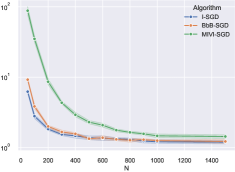
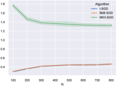
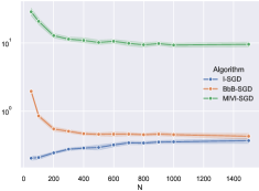
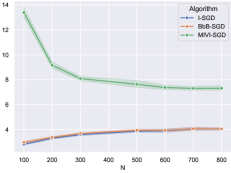
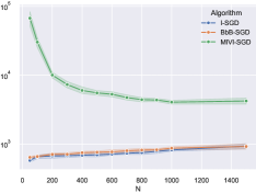
Figure 1: Convergence of $\mathbb{V}[\langle f,\eta_{t}^{N}\rangle]$ in the simple (left column) and complex (right column) setting, for $f_{mean}$ ($1^{st}$ line), $f_{std}$ ($2^{nd}$ line) and $f_{pred}$ ($3^{rd}$ line).

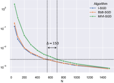
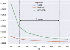
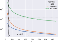
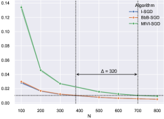
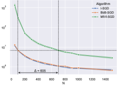
Figure 2: $\mathbb{V}[\langle f,\mu_{t}^{N}\rangle]$ with respect to $N$, in the simple (left column) and complex (right column) setting, for $f_{mean}$ ($1^{st}$ line), $f_{std}$ ($2^{nd}$ line) and $f_{pred}$ ($3^{rd}$ line).

This figure shows that, in the simple setting MiVI-SGD with $N=700$ obtains the same performance (in term of $\mathbb{V}[\langle f,\;\mu_{t}^{N}\rangle]$), than BbB-SGD and I-SGD with $N=620$ for $f_{mean}$, $N=210$ for $f_{std}$ and $N=380$. Similarly, in the complex setting MiVI-SGD with $N=700$ obtains the same performance (in term of $\mathbb{V}[\langle f,\;\mu_{t}^{N}\rangle]$), than BbB-SGD and I-SGD with $N=550$ for $f_{mean}$, $N=75$ for $f_{std}$ and $N=95$.

Consequently, in both settings, algorithm MiVI-SGD appears to be more efficient (in terms of the number of sampled vectors) than other algorithms for achieving the same value of $\mathbb{V}[\langle f,;\mu_{t}^{N}\rangle]$.

5 Conclusion

In this work, we have rigorously shown CLT for a two-layer BNN trained by variational inference with different SGD schemes. It appears that the idealized SGD and the most-commonly used Bayes-by-Backprop SGD schemes have the same fluctuation behaviors. i.e. driven by a SPDE with a $\mathfrak{G}$-process having the same covariance structure, in addition to admitting the same mean-field limit. Introduced in [DHG⁺23], the less costly Minimal VI SGD scheme exhibits a different fluctuation behavior, with a $\mathfrak{G}$-process of different covariance structure, which can be argued to lead to larger variances. Though, numerical experiments show that the trade-off between computational complexity and variance is still vastly in favour of the Minimal VI scheme. This opens the interesting perspective of exploring whether additional practical improvements can be derived from the asymptotic results at the mean-field level. This becomes even more intriguing and a justified approach given that neural networks appear to reach such limits rapidly.

Appendix A Central Limit Theorem: proof of Theorem 2

In all this section, the $\{\theta^{i}_{k},i\in\{1,\ldots,N\}\}$’s are generated by the algorithm (LABEL:eq.algo-batch), except in Section A.3 which, we recall, is dedicated to the study of the convergence of the sequences of martingale $(\sqrt{N}\mathbf{M}^{N})_{N}$ (see (24)). Recall the definition of the $\sigma$-algebra $\mathcal{F}_{k}^{N}$ in (8). We also recall the following paramount result which aims at giving uniform bounds, see Lemma 17 in [DHG⁺23] on the moments of the parameters $\{\theta^{i}_{k},i\in\{1,\ldots,N\}\}$ up to iteration $\lfloor NT\rfloor$, for a fixed $T>0$.

Lemma 1.

Assume A. Then, for all $T>0$ and all $p\geq 1$, there exists $C>0$ such that for all $N\geq 1$, $i\in\{1,\dots,N\}$ and $0\leq k\leq\lfloor NT\rfloor$, $\mathbf{E}[|\theta_{k}^{i}|^{p}]\leq C$.

Let us now recall some Sobolev embeddings which will be also used in the proof of Theorem 2. For $\mathfrak{M},\mathfrak{j}>(d+1)/2$ and $\mathfrak{k},\mathfrak{J}\geq 0$, $\mathcal{H}^{\mathfrak{M}+\mathfrak{J},\mathfrak{k}}(\mathbf{R}^{d+1})\hookrightarrow\mathcal{C}^{\mathfrak{J},\mathfrak{k}}(\mathbf{R}^{d+1})$ and $\mathcal{H}^{\mathfrak{M}+\mathfrak{J},\mathfrak{k}}(\mathbf{R}^{d+1})\hookrightarrow_{\mathrm{H.S.}}\mathcal{H}^{\mathfrak{J},\mathfrak{k}+\mathfrak{j}}(\mathbf{R}^{d+1})$ (see Section 2 in [FM97]). Recall $\mathfrak{J}_{3}=4\lceil\frac{d+1}{2}\rceil+8$ and $\mathfrak{j}_{3}=\lceil\frac{d+1}{2}\rceil+1$. Set $\mathfrak{J}_{0}=\lceil\frac{d+1}{2}\rceil+3,\ \mathfrak{J}_{1}=2\lceil\frac{d+1}{2}\rceil+4,\ \mathfrak{J}_{2}=3\lceil\frac{d+1}{2}\rceil+6$, and $\mathfrak{j}_{2}=2\lceil\frac{d+1}{2}\rceil+2,\ \mathfrak{j}_{1}=3\lceil\frac{d+1}{2}\rceil+4,\ \mathfrak{j}_{0}=4\lceil\frac{d+1}{2}\rceil+5$. Hence, the following Hilbert-Schmidt embeddings hold: $\mathcal{H}^{\mathfrak{J}_{3}-1\mathfrak{,}\mathfrak{j}_{3}}(\mathbf{R}^{d+1})\hookrightarrow_{\mathrm{H.S.}}\mathcal{H}^{\mathfrak{J}_{2},\mathfrak{j}_{2}}(\mathbf{R}^{d+1})$, $\mathcal{H}^{\mathfrak{J}_{2},\mathfrak{j}_{2}}(\mathbf{R}^{d+1})\hookrightarrow_{\mathrm{H.S.}}\mathcal{H}^{\mathfrak{J}_{1}+1,\mathfrak{j}_{1}-1}(\mathbf{R}^{d+1})$, $\mathcal{H}^{\mathfrak{J}_{1},\mathfrak{j}_{1}}(\mathbf{R}^{d+1})\hookrightarrow_{\mathrm{H.S.}}\mathcal{H}^{\mathfrak{J}_{0},\mathfrak{j}_{0}}(\mathbf{R}^{d+1})$. One also has the following continuous embeddings: $\mathcal{H}^{\mathfrak{J}_{0},\mathfrak{j}_{0}}(\mathbf{R}^{d+1})\hookrightarrow\mathcal{C}^{2,\mathfrak{j}_{0}}(\mathbf{R}^{d+1})$ and $\mathcal{H}^{\mathfrak{M},\mathfrak{j}}(\mathbf{R}^{d+1})\hookrightarrow\mathcal{H}^{\mathfrak{M},\mathfrak{j}+\mathfrak{k}}(\mathbf{R}^{d+1})$, where $\mathfrak{M},\mathfrak{j},\mathfrak{k}\geq 0$.

We finally recall some useful inequality which will be used throughout this work (see the proof of Lemma 1 in [DHG⁺23]) and which are direct consequences of A: for all $\theta\in\mathbf{R}^{d+1}$, $z\in\mathbf{R}^{d}$, and $(x,y)\in\mathsf{X}\times\mathsf{Y}$, it holds:

1. $|\phi(\theta,z,x)-y|\leq C$ and $|\nabla_{\theta}\phi(\theta,z,x)|\leq C|\mathrm{J}_{\theta}\Psi_{\theta}(z)|\leq C\mathfrak{b}(z)$ (where $\mathrm{J}_{\theta}$ denotes the Jacobian operator w.r.t. $\theta$).

In addition,

1. For all $x\in\mathsf{X}$,

   $$\mathfrak{H}(\cdot,x):\theta\mapsto\int_{\mathbf{R}^{d}}\phi(\theta,z,x)\gamma(z)\mathrm{d}z=\langle\phi(\theta,\cdot,x),\gamma\rangle$$ (15)

   is smooth and all its derivatives of non negative order are uniformly bounded over $\mathbf{R}^{d+1}$ w.r.t $x\in\mathsf{X}$.

Moreover, for any multi-index $\alpha\in\mathbf{N}^{d+1}$, (see Remark 1), it holds for some $C>0$ and all $\theta\in\mathbf{R}^{d+1}$:

$$|\partial_{\alpha}\mathscr{D}_{\mathrm{KL}}(q^{1}_{\theta}|P_{0}^{1})|\leq C(1+|\theta|)\text{ if }|\alpha|=1\text{ and }|\partial_{\alpha}\mathscr{D}_{\mathrm{KL}}(q^{1}_{\theta}|P_{0}^{1})|\leq C\text{ for }|\alpha|\geq 2.$$ (16)

A.1 Relative compactness of the fluctuation sequence $(\eta^{N})_{N\geq 1}$

Recall that the fluctuation process is defined by $\eta^{N}:t\in\mathbf{R}_{+}\mapsto\sqrt{N}(\mu^{N}_{t}-\bar{\mu}_{t})$, $N\geq 1$. The aim of this section is to prove the following relative compactness result on the sequence $(\eta^{N})_{N\geq 1}$.

Proposition 1.

Assume A. Then, $(\eta^{N})_{N\geq 1}$ is relatively compact in $\mathcal{D}(\mathbf{R}_{+},\mathcal{H}^{-\mathfrak{J}_{3}+1,\mathfrak{j}_{3}}(\mathbf{R}^{d+1}))$.

We mention that Proposition 1 also holds when the $\{\theta^{i}_{k},i\in\{1,\ldots,N\}\}$’s are generated by the two other algorithms (LABEL:eq.algo-ideal) and (LABEL:eq.algo-z1z2). Before starting the proof of Proposition 1, we need to introduce an auxiliary system of particles, this is the purpose of the next lemma.

For any $\mu\in\mathcal{P}(\mathcal{C}(\mathbf{R}_{+},\mathbf{R}^{d+1}))$, we consider $\mathscr{P}_{\mu}\in\mathcal{P}(\mathcal{C}(\mathbf{R}_{+},\mathbf{R}^{d+1}))$ defined as the law of the process $(X_{t})_{t\geq 0}$ solution to

$${\rm\mathbf{(E_{\mu})}}\begin{cases}\mathrm{d}X_{t}=-\kappa\int_{\mathsf{X}\times\mathsf{Y}}\langle\phi(\cdot,\cdot,x)-y,\mu_{t}\otimes\gamma\rangle\langle\nabla_{\theta}\phi(X_{t},\cdot,x),\gamma\rangle\pi(\mathrm{d}x,\mathrm{d}y)\mathrm{d}t-\kappa\nabla_{\theta}\mathscr{D}_{\mathrm{KL}}(q^{1}_{X_{t}}|P_{0}^{1})\mathrm{d}t,\\ X_{0}\sim\mu_{0}.\end{cases}$$

We then denote by $\mathscr{F}(\mu)$ the function $t\in\mathbf{R}_{+}\mapsto(\mathscr{P}_{\mu})_{t}=\mathscr{P}_{\mu}\circ\pi_{t}^{-1}$ the law $(X_{s})_{s\geq 0}$ at time $t$, where $\pi_{t}$ is the natural projection from $\mathcal{C}(\mathbf{R}_{+},\mathbf{R}^{d+1})$ to $\mathbf{R}$ define by $\pi_{t}(f)=f(t)$.

Lemma 2.

Assume A. Then, $\bar{\mu}=\mathscr{F}(\bar{\mu})$ (where $\bar{\mu}$ is given by Theorem 1), i.e. for the solution $(\bar{X}_{t})_{t\geq 0}$ of $\mathbf{(E_{\bar{\mu}})}$, it holds $\bar{X}_{t}\sim\bar{\mu}_{t}$ for all $t\geq 0$.

Proof.

We claim that $\mathscr{F}(\mu)\in\mathcal{C}(\mathbf{R}_{+},\mathcal{P}_{1}(\mathbf{R}^{d+1}))$, for all $\mu\in\mathcal{P}(\mathcal{C}(\mathbf{R}_{+},\mathbf{R}^{d+1}))$. Let us prove this claim. Let $(X_{t})_{t\geq 0}$ be the solution of $\mathbf{(E_{\mu})}$. Then, by I, II, and A, together with (16), there exists $c_{0}>0$ such that a.s. for all $t\geq 0$,

$$|X_{t}|\leq c_{0}(1+t)+c_{0}\int_{0}^{t}|X_{s}|\mathrm{d}s.$$

Therefore, a.s., for all $T>0$ and $0\leq t\leq T$, by Gronwall lemma, one has $|X_{t}|\leq c_{0}(1+T)e^{c_{0}T}$. With this bound, one deduces that there exists $c_{1}>0$ such that a.s. for all $0\leq s\leq t\leq T$, $|X_{t}-X_{s}|\leq c_{1}(1+T)e^{c_{1}T}(t-s)$, which proves the claim.

Let $\mu\in\mathcal{P}(\mathbf{R}^{d+1})$. Define $\mathscr{V}[\mu]:\mathbf{R}^{d+1}\to\mathbf{R}^{d+1}$ by:

$$\mathscr{V}[\mu](\theta)=-\kappa\int_{\mathsf{X}\times\mathsf{Y}}\langle\phi(\cdot,\cdot,x)-y,\mu\otimes\gamma\rangle\langle\nabla_{\theta}\phi(\theta,\cdot,x),\gamma\rangle\pi(\mathrm{d}x,\mathrm{d}y)-\kappa\nabla_{\theta}\mathscr{D}_{{\rm KL}}(q_{\theta}^{1}|P_{0}^{1}).$$ (17)

By the analysis carried out in Section B.3.2 in [DHG⁺23] (based on Th. 5.34 in [Vil03]), $\bar{\mu}$ is the unique weak solution in $\mathcal{C}(\mathbf{R}_{+},\mathcal{P}_{1}(\mathbf{R}^{d+1}))$ of the measure-valued equation

$$\begin{cases}\partial_{t}\mu^{*}_{t}=\mathrm{div}(\mathscr{V}[\bar{\mu}_{t}]\mu^{*}_{t})\\ \mu^{*}_{0}=\mu_{0}.\end{cases}$$ (18)

On the other hand, using the equality $g(X_{t})-g(X_{0})=\int_{0}^{t}\nabla g(X_{u})\cdot\frac{\mathrm{d}}{\mathrm{d}t}X_{u}\mathrm{d}u$ valid for any $\mathcal{C}^{1}$ function $g$ with compact support, together with $\mathbf{(E_{\mu})}$, we deduce that $\mathscr{F}(\bar{\mu})$ is a weak solution of (18). By uniqueness, $\bar{\mu}=\mathscr{F}(\bar{\mu})$. The proof is complete. ∎

Let us now introduce $N$ independent processes $\bar{X}^{i}$, $i\in\{1,\ldots,N\}$, solution to $\mathbf{(E_{\bar{\mu}})}$. It then holds thanks to Lemma 2, for all $i\in\{1,\ldots,N\}$ and $t\geq 0$:

$${\rm\mathbf{(S)}}\begin{cases}\mathrm{d}\bar{X}^{i}_{t}=-\kappa\int_{\mathsf{X}\times\mathsf{Y}}\langle\phi(\cdot,\cdot,x)-y,\bar{\mu}_{t}\otimes\gamma\rangle\langle\nabla_{\theta}\phi(\bar{X}^{i}_{t},\cdot,x),\gamma\rangle\pi(\mathrm{d}x,\mathrm{d}y)\mathrm{d}t-\kappa\nabla_{\theta}\mathscr{D}_{\mathrm{KL}}(q^{1}_{\bar{X}^{i}_{t}}|P_{0}^{1})\mathrm{d}t,\\ \bar{X}^{i}_{0}\sim\mu_{0},\ \bar{X}^{i}_{t}\sim\bar{\mu}_{t}.\end{cases}$$

Their empirical distribution is denoted by $\bar{\mu}_{t}^{N}=\frac{1}{N}\sum_{i=1}^{N}\delta_{\bar{X}_{t}^{i}}$, for $N\geq 1$ and $t\in\mathbf{R}_{+}$. Recall that from the proof of Lemma 2, there exists $c_{1}>0$ such that a.s. for all $0\leq s\leq t\leq T$ and all $i\in\{1,\dots,N\}$:

$$|\bar{X}^{i}_{t}|\leq c_{1}(1+T)e^{c_{1}T}\text{and }|\bar{X}^{i}_{t}-\bar{X}^{i}_{s}|\leq c_{1}(1+T)e^{c_{1}T}(t-s).$$ (19)

We now decompose $\eta^{N}$ using the following two processes:

$$\Upsilon^{N}:=\sqrt{N}(\mu^{N}-\bar{\mu}^{N})\ \text{and}\ \Theta^{N}:=\sqrt{N}(\bar{\mu}^{N}-\bar{\mu}).$$ (20)

We denote by $\mathcal{C}^{\mathfrak{J},\mathfrak{j}}(\mathbf{R}^{d+1})^{*}$ the dual space of $\mathcal{C}^{\mathfrak{J},\mathfrak{j}}(\mathbf{R}^{d+1})$ ($\mathfrak{J},\mathfrak{j}\geq 0$). One the one hand, $\bar{\mu}^{N}\in\mathcal{C}(\mathbf{R}_{+},\mathcal{C}^{1,\mathfrak{j}}(\mathbf{R}^{d+1})^{*})$, $\mathfrak{j}\geq 0$. This is indeed a direct consequence of (19). On the other hand, for any $\mathfrak{j}\geq 0$, $\mu^{N}\in\mathcal{D}(\mathbf{R}_{+},\mathcal{C}^{0,\mathfrak{j}}(\mathbf{R}^{d+1})^{*})$. Hence, it holds for all $\mathfrak{j}\geq 0$ a.s.

$$\Upsilon^{N}\in\mathcal{D}(\mathbf{R}_{+},\mathcal{C}^{1,\mathfrak{j}}(\mathbf{R}^{d+1})^{*}).$$ (21)

Concerning $\Theta^{N}$, we have the following result.

Lemma 3.

Assume A. Then, for any $\mathfrak{J}>1+(d+1)/2$ and $\mathfrak{k}\geq 0$, $\bar{\mu}^{N},\bar{\mu}\in\mathcal{C}(\mathbf{R}_{+},\mathcal{H}^{-\mathfrak{J},\mathfrak{k}}(\mathbf{R}^{d+1}))$. Therefore, a.s. $\Theta^{N}\in\mathcal{C}(\mathbf{R}_{+},\mathcal{H}^{-\mathfrak{J},\mathfrak{k}}(\mathbf{R}^{d+1}))$. Finally, (1) also holds for any test function $f\in\mathcal{H}^{\mathfrak{J},\mathfrak{k}}(\mathbf{R}^{d+1})$ ($\mathfrak{J}>1+(d+1)/2$ and $\mathfrak{k}\geq 0$).

Proof.

Let $\mathfrak{J}>1+(d+1)/2$ and $\mathfrak{k}\geq 0$. It then holds $\mathcal{H}^{\mathfrak{J},\mathfrak{k}}(\mathbf{R}^{d+1})\hookrightarrow\mathcal{C}^{1,\mathfrak{k}}(\mathbf{R}^{d+1})$. This implies that $\mathcal{C}^{1,\mathfrak{k}}(\mathbf{R}^{d+1})^{*}\hookrightarrow\mathcal{H}^{-\mathfrak{J},\mathfrak{k}}(\mathbf{R}^{d+1})$, and consequently, $\bar{\mu}^{N}\in\mathcal{C}(\mathbf{R}_{+},\mathcal{H}^{-\mathfrak{J},\mathfrak{k}}(\mathbf{R}^{d+1}))$.

Let us now prove that $\bar{\mu}\in\mathcal{C}(\mathbf{R}_{+},\mathcal{H}^{-\mathfrak{J},\mathfrak{k}}(\mathbf{R}^{d+1}))$ for $\mathfrak{k}\geq 0$. Set $\mathfrak{j}=\mathfrak{k}+1$. Recall that one can choose any $\gamma_{0}>1+\frac{d+1}{2}$ in Theorem 1. Pick thus such a $\gamma_{0}$ such that $\mathfrak{j}\leq\gamma_{0}$. We then have $\mathcal{H}^{\mathfrak{J},\mathfrak{j}-1}(\mathbf{R}^{d+1})\hookrightarrow\mathcal{C}^{1,\mathfrak{j}-1}(\mathbf{R}^{d+1})\hookrightarrow\mathcal{C}^{1,\gamma_{0}-1}(\mathbf{R}^{d+1})\hookrightarrow\mathcal{C}^{0,\gamma_{0}-1}(\mathbf{R}^{d+1})$. Since $\mu_{0}$ has compact support, $\mu_{0}\in\mathcal{C}^{0,\gamma_{0}-1}(\mathbf{R}^{d})^{*}\hookrightarrow\mathcal{H}^{-\mathfrak{J},\mathfrak{j}-1}(\mathbf{R}^{d})$. Let $f\in\mathcal{C}_{c}^{\infty}(\mathbf{R}^{d+1})$ and $0\leq s\leq t\leq T$. Thanks to (16) and Assumption A, we deduce that:

$$|\langle f,\bar{\mu}_{t}\rangle-\langle f,\bar{\mu}_{s}\rangle|\leq C|t-s|(\|f\|_{\mathcal{C}^{1,\gamma_{0}}}+\|f\|_{\mathcal{C}^{1,\gamma_{0}-1}})\sup_{u\in[0,T]}|\langle 1+|\cdot|^{\gamma_{0}},\bar{\mu}_{u}\rangle|$$

$$\leq C|t-s|\|f\|_{\mathcal{C}^{1,\gamma_{0}-1}}\sup_{u\in[0,T]}|\langle 1+|\cdot|^{\gamma_{0}},\bar{\mu}_{u}\rangle|$$

$$\leq C|t-s|\|f\|_{\mathcal{H}^{\mathfrak{J},\mathfrak{j}-1}}\sup_{u\in[0,T]}|\langle 1+|\cdot|^{\gamma_{0}},\bar{\mu}_{u}\rangle|.$$

We have that $\sup_{u\in[0,T]}|\langle 1+|\cdot|^{\gamma_{0}},\bar{\mu}_{u}\rangle|<+\infty$ since $u\geq 0\mapsto\langle 1+|\cdot|^{\gamma_{0}},\bar{\mu}_{u}\rangle\in\mathcal{D}(\mathbf{R}_{+},\mathbf{R})$ (this follows from the fact that $\bar{\mu}\in\mathcal{D}(\mathbf{R}_{+},\mathcal{P}_{\gamma_{0}}(\mathbf{R}^{d}))$ together with  Th. 6.9 in [Vil09]). We have thus proved that $\bar{\mu}_{t}\in\mathcal{H}^{-\mathfrak{J},\mathfrak{j}-1}(\mathbf{R}^{d})$ and $|\langle f,\bar{\mu}_{t}\rangle-\langle f,\bar{\mu}_{s}\rangle|\leq C|t-s|\|f\|_{\mathcal{H}^{\mathfrak{J},\mathfrak{j}-1}}$. This proves that $\bar{\mu}\in\mathcal{C}(\mathbf{R}_{+},\mathcal{H}^{-\mathfrak{J},\mathfrak{j}-1}(\mathbf{R}^{d+1}))$. The last claim is obtained by a density argument and the fact that $\mathcal{H}^{\mathfrak{J},\mathfrak{j}-1}(\mathbf{R}^{d+1})\hookrightarrow\mathcal{C}^{1,\gamma_{0}-1}(\mathbf{R}^{d+1})$. ∎

Lemma 4.

Assume A. For all $T>0$, we have

$$\sup_{N\geq 1}\sup_{t\in[0,T]}\mathbf{E}[\|\Theta_{t}^{N}\|_{\mathcal{H}^{-\mathfrak{J}_{1},\mathfrak{j}_{1}}}^{2}+\|\Upsilon_{t}^{N}\|_{\mathcal{H}^{-\mathfrak{J}_{1},\mathfrak{j}_{1}}}^{2}]<+\infty.$$

In particular, $\sup_{N\geq 1}\sup_{t\in[0,T]}\mathbf{E}[\|\eta_{t}^{N}\|_{\mathcal{H}^{-\mathfrak{J}_{1},\mathfrak{j}_{1}}}^{2}]<+\infty$.

Proof.

Let $T>0$. Pick $t\in[0,T]$, $N\geq 1$, and $f\in\mathcal{H}^{\mathfrak{J}_{1},\mathfrak{j}_{1}}(\mathbf{R}^{d})$. On the one hand, since $(f(\bar{X}_{t}^{j})-\langle f,\bar{\mu}_{t}\rangle)_{j=1,\ldots,N}$ are independent centered random variables, one deduces that $\textbf{E}[\langle f,\Theta_{t}^{N}\rangle^{2}]\leq\frac{2}{N}\sum_{i=1}^{N}(\textbf{E}\big{[}|f(\bar{X}_{t}^{i})|^{2}\big{]}+|\langle f,\bar{\mu}_{t}\rangle|^{2})\leq C_{T}\|f\|_{\mathcal{H}^{\mathfrak{J}_{0},\mathfrak{j}_{0}}}^{2}$, where the last inequality is a consequence of (19) together with $\mathcal{H}^{\mathfrak{J}_{0},\mathfrak{j}_{0}}(\mathbf{R}^{d+1})\hookrightarrow\mathcal{C}^{0,\mathfrak{j}_{0}}(\mathbf{R}^{d+1})$ and $\bar{\mu}\in\mathcal{C}(\mathbf{R}_{+},\mathcal{H}^{-\mathfrak{J}_{0},\mathfrak{j}_{0}}(\mathbf{R}^{d+1}))$ (see Lemma 3). Using also the embedding $\mathcal{H}^{\mathfrak{J}_{1},\mathfrak{j}_{1}}(\mathbf{R}^{d+1})\hookrightarrow_{\mathrm{H.S.}}\mathcal{H}^{\mathfrak{J}_{0},\mathfrak{j}_{0}}(\mathbf{R}^{d+1})$ and considering an orthonormal basis of $\mathcal{H}^{\mathfrak{J}_{1},\mathfrak{j}_{1}}(\mathbf{R}^{d+1})$, one deduces the desired upper bound on $\Theta^{N}$.

Let us now derive the bound on the second order moment of $\Upsilon^{N}$. To this end, introduce an orthonormal basis $(f_{a})_{a\geq 1}$ of $\mathcal{H}^{\mathfrak{J}_{1},\mathfrak{j}_{1}}(\mathbf{R}^{d+1})$. One then has:

$$\|\Upsilon_{t}^{N}\|_{\mathcal{H}^{-\mathfrak{J}_{1},\mathfrak{j}_{1}}}^{2}=\sum_{a\geq 1}\langle f_{a},\Upsilon_{t}^{N}\rangle^{2}.$$ (22)

Recall $\mathcal{H}^{\mathfrak{J}_{0},\mathfrak{j}_{0}}(\mathbf{R}^{d+1})\hookrightarrow\mathcal{C}^{2,\mathfrak{j}_{0}}(\mathbf{R}^{d+1})$. We have, by (S) and the fact that $f\in\mathcal{C}^{2,\mathfrak{j}_{0}}(\mathbf{R}^{d+1})$,

$$\langle f,\bar{\mu}_{t}^{N}\rangle=\langle f,\bar{\mu}_{0}^{N}\rangle -\kappa\int_{0}^{t}\int_{\mathsf{X}\times\mathsf{Y}}\langle\phi(\cdot,\cdot,x)-y,\bar{\mu}_{s}\otimes\gamma\rangle\langle\nabla f\cdot\nabla_{\theta}\phi(\cdot,\cdot,x),\bar{\mu}_{s}^{N}\otimes\gamma\rangle\pi(\mathrm{d}x,\mathrm{d}y)\mathrm{d}s$$

$$-\kappa\int_{0}^{t}\langle\nabla f\cdot\nabla_{\theta}\mathscr{D}_{\mathrm{KL}}(q_{\cdot}^{1}|P_{0}^{1}),\bar{\mu}_{s}^{N}\rangle\mathrm{d}s.$$ (23)

We now set for $k\geq 0$ and $g\in\mathcal{C}^{2,\mathfrak{j}}(\mathbf{R}^{d+1})$ ($\mathfrak{j}\geq 0$):

1. $\mathbf{D}_{k}^{N}[g]:=-\frac{\kappa}{N^{3}}\sum_{i=1}^{N}\sum_{j=1,j\neq i}^{N}\int_{\mathsf{X}\times\mathsf{Y}}\big{(}\big{\langle}\phi(\theta_{k}^{j},\cdot,x),\gamma\big{\rangle}-y\big{)}\big{\langle}\nabla_{\theta}g(\theta_{k}^{i})\cdot\nabla_{\theta}\phi(\theta_{k}^{i},\cdot,x),\gamma\big{\rangle}\pi(\mathrm{d}x,\mathrm{d}y)-\frac{\kappa}{N^{2}}\int_{\mathsf{X}\times\mathsf{Y}}\big{\langle}(\phi(\cdot,\cdot,x)-y)\nabla_{\theta}g\cdot\nabla_{\theta}\phi(\cdot,\cdot,x),\nu_{k}^{N}\otimes\gamma\big{\rangle}\pi(\mathrm{d}x,\mathrm{d}y)$.

2. $\mathbf{M}_{k}^{N}[g]=-\frac{\kappa}{N^{3}}\sum_{i,j=1}^{N}(\phi(\theta_{k}^{j},\mathsf{Z}_{k}^{j},x_{k})-y_{k})\nabla_{\theta}g(\theta_{k}^{i})\cdot\nabla_{\theta}\phi(\theta_{k}^{i},\mathsf{Z}_{k}^{i},x_{k})-\mathbf{D}_{k}^{N}[g]$.

3. $\mathbf{R}_{k}^{N}[g]:=\frac{1}{2N}\sum_{i=1}^{N}(\theta_{k+1}^{i}-\theta_{k}^{i})^{T}\nabla^{2}g(\widehat{\theta_{k}^{i}})(\theta_{k+1}^{i}-\theta_{k}^{i})$ is the rest of the second order Taylor expansion of $\frac{1}{N}\sum_{k=1}^{N}f(\theta_{k+1}^{i})-f(\theta_{k}^{i})$ (the point $\widehat{\theta_{k}^{i}}$ lies in $[\theta_{k+1}^{i},\theta_{k}^{i}]$).

Note that $\mathbf{D}_{k}^{N}[g]$ and $\mathbf{M}_{k}^{N}[g]$ are well defined for $g\in\mathcal{C}^{1,\mathfrak{j}}(\mathbf{R}^{d+1})$ ($\mathfrak{j}\geq 0$). For $t\geq 0$, we also define:

$$\mathbf{R}_{t}^{N}[g]:=\sum_{k=0}^{\lfloor Nt\rfloor-1}\mathbf{R}_{k}^{N}[g]\ \ \text{and}\ \ \mathbf{M}_{t}^{N}[g]:=\sum_{k=0}^{\lfloor Nt\rfloor-1}\mathbf{M}_{k}^{N}[g].$$ (24)

Let $t\geq 0$. With these definitions, we recall that from Eq. (53) in [DHG⁺23], there exist $\widehat{\theta_{k}^{i}}$ ($i=1,\ldots,N$ and $k=0,\ldots,\lfloor Nt\rfloor-1$) such that for $g\in\mathcal{C}^{2,\mathfrak{j}_{0}}(\mathbf{R}^{d+1})$:

$$\langle g,\mu_{t}^{N}\rangle-\langle g,\mu_{0}^{N}\rangle =-\kappa\int_{0}^{t}\int_{\mathsf{X}\times\mathsf{Y}}\langle\phi(\cdot,\cdot,x)-y,\mu_{s}^{N}\otimes\gamma\rangle\langle\nabla_{\theta}g\cdot\nabla_{\theta}\phi(\cdot,\cdot,x),\mu_{s}^{N}\otimes\gamma\rangle\pi(\mathrm{d}x,\mathrm{d}y)\mathrm{d}s$$

$$\quad-\kappa\int_{0}^{t}\big{\langle}\nabla_{\theta}g\cdot\nabla_{\theta}\mathscr{D}_{{\rm KL}}(q_{\,{}_{\cdot}}^{1}|P_{0}^{1}),\mu_{s}^{N}\big{\rangle}\mathrm{d}s$$

$$\quad+\frac{\kappa}{N}\int_{0}^{t}\int_{\mathsf{X}\times\mathsf{Y}}\Big{\langle}\langle\phi(\cdot,\cdot,x)-y,\gamma\rangle\langle\nabla_{\theta}g\cdot\nabla_{\theta}\phi(\cdot,\cdot,x),\gamma\rangle,\mu_{s}^{N}\Big{\rangle}\pi(\mathrm{d}x,\mathrm{d}y)\mathrm{d}s$$

$$\quad-\frac{\kappa}{N}\int_{0}^{t}\int_{\mathsf{X}\times\mathsf{Y}}\Big{\langle}(\phi(\cdot,\cdot,x)-y)\nabla_{\theta}g\cdot\nabla_{\theta}\phi(\cdot,\cdot,x),\mu_{s}^{N}\otimes\gamma\Big{\rangle}\pi(\mathrm{d}x,\mathrm{d}y)\mathrm{d}s$$

$$\quad+\mathbf{M}_{t}^{N}[g]+\mathbf{W}_{t}^{N}[g]+\mathbf{R}_{t}^{N}[g],$$ (25)

where $\mathbf{W}_{t}^{N}[f]:=-\mathbf{V}_{t}^{N}[f]+\kappa\int^{t}_{\frac{\lfloor Nt\rfloor}{N}}\big{\langle}\nabla_{\theta}f\cdot\nabla_{\theta}\mathscr{D}_{{\rm KL}}(q_{\,{}_{\cdot}}^{1}|P_{0}^{1}),\mu_{s}^{N}\big{\rangle}\mathrm{d}s$ and

$$\mathbf{V}_{t}^{N}[f] :=-\kappa\int^{t}_{\frac{\lfloor Nt\rfloor}{N}}\int_{\mathsf{X}\times\mathsf{Y}}\langle\phi(\cdot,\cdot,x)-y,\mu_{s}^{N}\otimes\gamma\rangle\langle\nabla_{\theta}f\cdot\nabla_{\theta}\phi(\cdot,\cdot,x),\mu_{s}^{N}\otimes\gamma\rangle\pi(\mathrm{d}x,\mathrm{d}y)\mathrm{d}s$$

$$\quad+\frac{\kappa}{N}\int^{t}_{\frac{\lfloor Nt\rfloor}{N}}\int_{\mathsf{X}\times\mathsf{Y}}\Big{\langle}\langle\phi(\cdot,\cdot,x)-y,\gamma\rangle\langle\nabla_{\theta}f\cdot\nabla_{\theta}\phi(\cdot,\cdot,x),\gamma\rangle,\mu_{s}^{N}\Big{\rangle}\pi(\mathrm{d}x,\mathrm{d}y)\mathrm{d}s$$

$$\quad-\frac{\kappa}{N}\int^{t}_{\frac{\lfloor Nt\rfloor}{N}}\int_{\mathsf{X}\times\mathsf{Y}}\Big{\langle}(\phi(\cdot,\cdot,x)-y)\nabla_{\theta}f\cdot\nabla_{\theta}\phi(\cdot,\cdot,x),\mu_{s}^{N}\otimes\gamma\Big{\rangle}\pi(\mathrm{d}x,\mathrm{d}y)\mathrm{d}s.$$

Hence, since by definition $\Upsilon^{N}=\sqrt{N}(\mu^{N}-\bar{\mu}^{N})$, one has for all $t\in\mathbf{R}_{+}$, using (A.1) and (A.1) together with the fact that $\langle f,\mu_{0}^{N}\rangle=\langle f,\bar{\mu}_{0}^{N}\rangle$:

$$\langle f,\Upsilon_{t}^{N}\rangle =-\kappa\int_{0}^{t}\int_{\mathsf{X}\times\mathsf{Y}}\langle\phi(\cdot,\cdot,x)-y,\mu_{s}^{N}\otimes\gamma\rangle\langle\nabla_{\theta}f\cdot\nabla_{\theta}\phi(\cdot,\cdot,x),\Upsilon_{s}^{N}\otimes\gamma\rangle\pi(\mathrm{d}x,\mathrm{d}y)\mathrm{d}s$$

$$\quad-\kappa\int_{0}^{t}\int_{\mathsf{X}\times\mathsf{Y}}\langle\phi(\cdot,\cdot,x),\Upsilon_{s}^{N}\otimes\gamma\rangle\langle\nabla_{\theta}f\cdot\nabla_{\theta}\phi(\cdot,\cdot,x),\bar{\mu}_{s}^{N}\otimes\gamma\rangle\pi(\mathrm{d}x,\mathrm{d}y)\mathrm{d}s$$

$$\quad-\kappa\int_{0}^{t}\int_{\mathsf{X}\times\mathsf{Y}}\langle\phi(\cdot,\cdot,x),\sqrt{N}(\bar{\mu}_{s}^{N}-\bar{\mu}_{s})\otimes\gamma\rangle\langle\nabla_{\theta}f\cdot\nabla_{\theta}\phi(\cdot,\cdot,x),\bar{\mu}_{s}^{N}\otimes\gamma\rangle\pi(\mathrm{d}x,\mathrm{d}y)\mathrm{d}s$$

$$\quad-\kappa\int_{0}^{t}\langle\nabla_{\theta}f\cdot\nabla_{\theta}\mathscr{D}_{\mathrm{KL}}(q^{1}_{\cdot}|P_{0}^{1}),\Upsilon_{s}^{N}\rangle\mathrm{d}s$$

$$\quad+\frac{\kappa}{\sqrt{N}}\int_{0}^{t}\int_{\mathsf{X}\times\mathsf{Y}}\Big{\langle}\langle\phi(\cdot,\cdot,x)-y,\gamma\rangle\langle\nabla_{\theta}f\cdot\nabla_{\theta}\phi(\cdot,\cdot,x),\gamma\rangle,\mu_{s}^{N}\Big{\rangle}\pi(\mathrm{d}x,\mathrm{d}y)\mathrm{d}s$$

$$\quad-\frac{\kappa}{\sqrt{N}}\int_{0}^{t}\int_{\mathsf{X}\times\mathsf{Y}}\Big{\langle}(\phi(\cdot,\cdot,x)-y)\nabla_{\theta}f\cdot\nabla_{\theta}\phi(\cdot,\cdot,x),\mu_{s}^{N}\otimes\gamma\Big{\rangle}\pi(\mathrm{d}x,\mathrm{d}y)\mathrm{d}s$$

$$\quad+\sqrt{N}\mathbf{M}_{t}^{N}[f]+\sqrt{N}\mathbf{W}_{t}^{N}[f]+\sqrt{N}\mathbf{R}_{t}^{N}[f].$$ (26)

Using II, when $\mathfrak{j}>\frac{d+1}{2}$, one has $\mathfrak{H}(\cdot,x)\in\mathcal{H}^{\mathfrak{J},\mathfrak{j}}(\mathbf{R}^{d+1})$ for all $\mathfrak{J}\geq 0$, and it holds:

$$\sup_{x\in\mathsf{X}}\big{\|}\mathfrak{H}(.,x)\big{\|}_{\mathcal{H}^{\mathfrak{J},\mathfrak{j}}}<+\infty.$$ (27)

By Lemma B.3 in [DGMN22], one has, for all $t\in\mathbf{R}_{+}$,

$$\langle f,\Upsilon_{t}^{N}\rangle^{2}\leq\mathbf{A}_{t}^{N}[f]+\mathbf{B}_{t}^{N}[f],$$ (28)

where

$$\mathbf{A}_{t}^{N}[f] =-2\kappa\int_{0}^{t}\int_{\mathsf{X}\times\mathsf{Y}}\langle f,\Upsilon_{s}^{N}\rangle\langle\phi(\cdot,\cdot,x)-y,\mu_{s}^{N}\otimes\gamma\rangle\langle\nabla_{\theta}f\cdot\nabla_{\theta}\phi(\cdot,\cdot,x),\Upsilon_{s}^{N}\otimes\gamma\rangle\pi(\mathrm{d}x,\mathrm{d}y)\mathrm{d}s$$

$$\quad-2\kappa\int_{0}^{t}\int_{\mathsf{X}\times\mathsf{Y}}\langle f,\Upsilon_{s}^{N}\rangle\langle\phi(\cdot,\cdot,x),\Upsilon_{s}^{N}\otimes\gamma\rangle\langle\nabla_{\theta}f\cdot\nabla_{\theta}\phi(\cdot,\cdot,x),\bar{\mu}_{s}^{N}\otimes\gamma\rangle\pi(\mathrm{d}x,\mathrm{d}y)\mathrm{d}s$$

$$\quad-2\kappa\int_{0}^{t}\int_{\mathsf{X}\times\mathsf{Y}}\langle f,\Upsilon_{s}^{N}\rangle\langle\phi(\cdot,\cdot,x),\sqrt{N}(\bar{\mu}_{s}^{N}-\bar{\mu}_{s})\otimes\gamma\rangle\langle\nabla_{\theta}f\cdot\nabla_{\theta}\phi(\cdot,\cdot,x),\bar{\mu}_{s}^{N}\otimes\gamma\rangle\pi(\mathrm{d}x,\mathrm{d}y)\mathrm{d}s$$

$$\quad-2\kappa\int_{0}^{t}\langle f,\Upsilon_{s}^{N}\rangle\langle\nabla_{\theta}f\cdot\nabla_{\theta}\mathscr{D}_{\mathrm{KL}}(q^{1}_{\cdot}|P_{0}^{1}),\Upsilon_{s}^{N}\rangle\mathrm{d}s$$

$$\quad+\frac{2\kappa}{\sqrt{N}}\int_{0}^{t}\int_{\mathsf{X}\times\mathsf{Y}}\langle f,\Upsilon_{s}^{N}\rangle\Big{\langle}\langle\phi(\cdot,\cdot,x)-y,\gamma\rangle\langle\nabla_{\theta}f\cdot\nabla_{\theta}\phi(\cdot,\cdot,x),\gamma\rangle,\mu_{s}^{N}\Big{\rangle}\pi(\mathrm{d}x,\mathrm{d}y)\mathrm{d}s$$

$$\quad-\frac{2\kappa}{\sqrt{N}}\int_{0}^{t}\int_{\mathsf{X}\times\mathsf{Y}}\langle f,\Upsilon_{s}^{N}\rangle\Big{\langle}(\phi(\cdot,\cdot,x)-y)\nabla_{\theta}f\cdot\nabla_{\theta}\phi(\cdot,\cdot,x),\mu_{s}^{N}\otimes\gamma\Big{\rangle}\pi(\mathrm{d}x,\mathrm{d}y)\mathrm{d}s$$ (29)

and

$$\mathbf{B}_{t}^{N}[f] =\sum_{k=0}^{\lfloor Nt\rfloor-1}\Big{[}2\langle f,\Upsilon_{\frac{k+1}{N}^{-}}^{N}\rangle\sqrt{N}\mathbf{R}_{k}^{N}[f]+3N\mathbf{R}_{k}^{N}[f]^{2}\Big{]}+\sum_{k=0}^{\lfloor Nt\rfloor-1}\Big{[}2\langle f,\Upsilon_{\frac{k+1}{N}^{-}}^{N}\rangle\sqrt{N}\mathbf{M}_{k}^{N}[f]+3N\mathbf{M}_{k}^{N}[f]^{2}\Big{]}$$

$$\quad+\sum_{k=0}^{\lfloor Nt\rfloor-1}\Big{[}2\langle f,\Upsilon_{\frac{k+1}{N}^{-}}^{N}\rangle\mathbf{a}_{k}^{N}[f]+3\mathbf{a}_{k}^{N}[f]^{2}\Big{]}-2\sqrt{N}\int_{0}^{t}\langle f,\Upsilon_{s}^{N}\rangle\mathbf{L}_{s}^{N}[f]\mathrm{d}s,$$

with, for $s\in[0,t]$,

$$\mathbf{L}_{s}^{N}[f] =-\kappa\int_{\mathsf{X}\times\mathsf{Y}}\langle\phi(\cdot,\cdot,x)-y,\mu_{s}^{N}\otimes\gamma\rangle\langle\nabla_{\theta}f\cdot\nabla_{\theta}\phi(\cdot,\cdot,x),\mu_{s}^{N}\otimes\gamma\rangle\pi(\mathrm{d}x,\mathrm{d}y)$$

$$+\frac{\kappa}{N}\int_{\mathsf{X}\times\mathsf{Y}}\Big{\langle}\langle\phi(\cdot,\cdot,x)-y,\gamma\rangle\langle\nabla_{\theta}f\cdot\nabla_{\theta}\phi(\cdot,\cdot,x),\gamma\rangle,\mu_{s}^{N}\Big{\rangle}\pi(\mathrm{d}x,\mathrm{d}y)$$

$$-\frac{\kappa}{N}\int_{\mathsf{X}\times\mathsf{Y}}\Big{\langle}(\phi(\cdot,\cdot,x)-y)\nabla_{\theta}f\cdot\nabla_{\theta}\phi(\cdot,\cdot,x),\mu_{s}^{N}\otimes\gamma\Big{\rangle}\pi(\mathrm{d}x,\mathrm{d}y)$$

$$-\kappa\langle\nabla_{\theta}f\cdot\nabla_{\theta}\mathscr{D}_{\mathrm{KL}}(q^{1}_{\cdot}|P_{0}^{1}),\mu_{s}^{N}\rangle$$

and, for $0\leq k<\lfloor Nt\rfloor$, $\mathbf{a}_{k}^{N}[f]=\sqrt{N}\int_{\frac{k}{N}}^{\frac{k+1}{N}}\mathbf{L}_{s}^{N}[f]\mathrm{d}s$. By (22) and (28),

$$\|\Upsilon_{t}^{N}\|_{\mathcal{H}^{-\mathfrak{J}_{1},\mathfrak{j}_{1}}}^{2}\leq\sum_{a\geq 1}\mathbf{A}_{t}^{N}[f_{a}]+\mathbf{B}_{t}^{N}[f_{a}].$$ (30)

Using Lemma 7, one deduces that:

$$\sum_{a\geq 1}\mathbf{E}[\mathbf{A}_{t}^{N}[f_{a}]+\mathbf{B}_{t}^{N}[f_{a}]]\leq C_{T}+C_{T}\int_{0}^{t}\mathbf{E}[\|\Upsilon_{s}^{N}\|_{\mathcal{H}^{-\mathfrak{J}_{1},\mathfrak{j}_{1}}}^{2}]\mathrm{d}s$$ (31)

Hence, by (30) and (31),

$$\mathbf{E}[\|\Upsilon_{t}^{N}\|_{\mathcal{H}^{-\mathfrak{J}_{1},\mathfrak{j}_{1}}}^{2}]\leq C_{T}+C_{T}\int_{0}^{t}\mathbf{E}[\|\Upsilon_{s}^{N}\|_{\mathcal{H}^{-\mathfrak{J}_{1},\mathfrak{j}_{1}}}^{2}]\mathrm{d}s.$$ (32)

Using Gronwall’s lemma yields the desired moment estimate on $\Upsilon^{N}$. ∎

The following lemma provides the compact containment condition we need to prove that $(\eta^{N})_{N\geq 1}$ is relatively compact in $\mathcal{D}(\mathbf{R}_{+},\mathcal{H}^{-\mathfrak{J}_{3}+1,\mathfrak{j}_{3}}(\mathbf{R}^{d+1}))$.

Lemma 5.

Assume A. Then, for all $T>0$, $\sup_{N\geq 1}\mathbf{E}[\sup_{t\in[0,T]}\|\eta_{t}^{N}\|_{\mathcal{H}^{-\mathfrak{J}_{2},\mathfrak{j}_{2}}}^{2}]<+\infty$.

Proof.

Let $T>0$ and $N\geq 1$. Consider an orthonormal basis $(f_{a})_{a\geq 1}$ of $\mathcal{H}^{\mathfrak{J}_{2},\mathfrak{j}_{2}}(\mathbf{R}^{d+1})$ and $f\in\mathcal{H}^{\mathfrak{J}_{2},\mathfrak{j}_{2}}(\mathbf{R}^{d+1})$. From (A.1) and using Jensen’s inequality,

$$\sup_{t\in[0,T]}\langle f,\Upsilon_{t}^{N}\rangle^{2} \leq C\int_{0}^{T}\int_{\mathsf{X}\times\mathsf{Y}}|\langle\phi(\cdot,\cdot,x)-y,\mu_{s}^{N}\otimes\gamma\rangle\langle\nabla_{\theta}f\cdot\nabla_{\theta}\phi(\cdot,\cdot,x),\Upsilon_{s}^{N}\otimes\gamma\rangle|^{2}\pi(\mathrm{d}x,\mathrm{d}y)\mathrm{d}s$$

$$\quad+C\int_{0}^{T}\int_{\mathsf{X}\times\mathsf{Y}}|\langle\phi(\cdot,\cdot,x),\Upsilon_{s}^{N}\otimes\gamma\rangle\langle\nabla_{\theta}f\cdot\nabla_{\theta}\phi(\cdot,\cdot,x),\bar{\mu}_{s}^{N}\otimes\gamma\rangle|^{2}\pi(\mathrm{d}x,\mathrm{d}y)\mathrm{d}s$$

$$\quad+C\int_{0}^{T}\int_{\mathsf{X}\times\mathsf{Y}}|\langle\phi(\cdot,\cdot,x),\sqrt{N}(\bar{\mu}_{s}^{N}-\bar{\mu}_{s})\otimes\gamma\rangle\langle\nabla_{\theta}f\cdot\nabla_{\theta}\phi(\cdot,\cdot,x),\bar{\mu}_{s}^{N}\otimes\gamma\rangle|^{2}\pi(\mathrm{d}x,\mathrm{d}y)\mathrm{d}s$$

$$\quad+C\int_{0}^{T}|\langle\nabla_{\theta}f\cdot\nabla_{\theta}\mathscr{D}_{\mathrm{KL}}(q^{1}_{\cdot}|P_{0}^{1}),\Upsilon_{s}^{N}\rangle|^{2}\mathrm{d}s$$

$$\quad+\frac{C}{N}\int_{0}^{T}\int_{\mathsf{X}\times\mathsf{Y}}\Big{\langle}\langle\phi(\cdot,\cdot,x)-y,\gamma\rangle\langle\nabla_{\theta}f\cdot\nabla_{\theta}\phi(\cdot,\cdot,x),\gamma\rangle,\mu_{s}^{N}\Big{\rangle}^{2}\pi(\mathrm{d}x,\mathrm{d}y)\mathrm{d}s$$

$$\quad+\frac{C}{N}\int_{0}^{T}\int_{\mathsf{X}\times\mathsf{Y}}\Big{\langle}(\phi(\cdot,\cdot,x)-y)\nabla_{\theta}f\cdot\nabla_{\theta}\phi(\cdot,\cdot,x),\mu_{s}^{N}\otimes\gamma\Big{\rangle}^{2}\pi(\mathrm{d}x,\mathrm{d}y)\mathrm{d}s$$

$$\quad+N\sup_{t\in[0,T]}\mathbf{M}_{t}^{N}[f]^{2}+N\sup_{t\in[0,T]}\mathbf{W}_{t}^{N}[f]^{2}+N\sup_{t\in[0,T]}\mathbf{R}_{t}^{N}[f]^{2}.$$ (33)

Let us now provide upper bounds on each term appearing in the right-hand side of (A.1). Let us consider the first term in the right-hand side of (A.1). By II, for all $\mathfrak{J}\geq 1$ and $\mathfrak{j}\geq 0$,

$$\sup_{g\in\mathcal{H}^{\mathfrak{J},\mathfrak{j}}(\mathbf{R}^{d+1}),\|g\|_{\mathcal{H}^{\mathfrak{J},\mathfrak{j}}}=1}\ \sup_{x\in\mathsf{X}}\big{\|}\nabla_{\theta}g\cdot\mathfrak{H}(\cdot,x)\big{\|}_{\mathcal{H}^{\mathfrak{J}-1,\mathfrak{j}}}<+\infty.$$ (34)

By (48), (34), the embedding $\mathcal{H}^{\mathfrak{J}_{2},\mathfrak{j}_{2}}(\mathbf{R}^{d+1})\hookrightarrow\mathcal{H}^{\mathfrak{J}_{1}+1,\mathfrak{j}_{1}}(\mathbf{R}^{d+1})$ together with Lemma 4, we have, for all $s\in[0,T]$,

$$\mathbf{E}\Big{[}\int_{\mathsf{X}\times\mathsf{Y}}|\langle\phi(\cdot,\cdot,x)-y,\mu_{s}^{N}\otimes\gamma\rangle\langle\nabla_{\theta}f\cdot\nabla_{\theta}\phi(\cdot,\cdot,x),\Upsilon_{s}^{N}\otimes\gamma\rangle|^{2}\pi(\mathrm{d}x,\mathrm{d}y)\Big{]}$$

$$\leq C\mathbf{E}\Big{[}\int_{\mathsf{X}\times\mathsf{Y}}\big{\|}\nabla_{\theta}f\cdot\mathfrak{H}(\cdot,x)\big{\|}_{\mathcal{H}^{\mathfrak{J}_{1},\mathfrak{j}_{1}}}^{2}\|\Upsilon_{s}^{N}\|_{\mathcal{H}^{-\mathfrak{J}_{1},\mathfrak{j}_{1}}}^{2}\pi(\mathrm{d}x,\mathrm{d}y)\Big{]}$$

$$\leq C\|f\|_{\mathcal{H}^{\mathfrak{J}_{1}+1,\mathfrak{j}_{1}}}^{2}\mathbf{E}[\|\Upsilon_{s}^{N}\|_{\mathcal{H}^{-\mathfrak{J}_{1},\mathfrak{j}_{1}}}^{2}]\leq C\|f\|_{\mathcal{H}^{\mathfrak{J}_{1}+1,\mathfrak{j}_{1}}}^{2}.$$ (35)

Let us now deal with the second term in the right hand side of (A.1). Using (27), Lemma 4 and (50), and Sobolev embeddings, we have, for all $s\in[0,T]$,

$$\mathbf{E}[|\langle\phi(\cdot,\cdot,x),\Upsilon_{s}^{N}\otimes\gamma\rangle\langle\nabla_{\theta}f\cdot\nabla_{\theta}\phi(\cdot,\cdot,x),\bar{\mu}_{s}^{N}\otimes\gamma\rangle|^{2}]\leq C\|f\|^{2}_{\mathcal{H}^{\mathfrak{J}_{1},\mathfrak{j}_{1}}}\mathbf{E}[\|\Upsilon_{s}^{N}\|_{\mathcal{H}^{-\mathfrak{J}_{1},\mathfrak{j}_{1}}}^{2}]\leq C\|f\|^{2}_{\mathcal{H}^{\mathfrak{J}_{1},\mathfrak{j}_{1}}},$$

which provides the required upper bound.

We now consider the t third term in the r.h.s. of (A.1). We have, using (50) and (51), together with the embedding $\mathcal{H}^{\mathfrak{J}_{0},\mathfrak{j}_{0}}(\mathbf{R}^{d+1})\hookrightarrow\mathcal{C}^{1,\mathfrak{j}_{0}}(\mathbf{R}^{d+1})$, for all $s\in[0,T]$,

$$\mathbf{E}[|\langle\phi(\cdot,\cdot,x),\sqrt{N}(\bar{\mu}_{s}^{N}-\bar{\mu}_{s})\otimes\gamma\rangle\langle\nabla_{\theta}f\cdot\nabla_{\theta}\phi(\cdot,\cdot,x),\bar{\mu}_{s}^{N}\otimes\gamma\rangle|^{2}]\leq C\|f\|_{\mathcal{H}^{\mathfrak{J}_{0},\mathfrak{j}_{0}}}^{2}.$$

We now turn to the fourth term in (A.1). Note first that by (16), we have that $\nabla_{\theta}g\cdot\nabla_{\theta}\mathscr{D}_{\mathrm{KL}}(q^{1}_{\cdot}|P_{0}^{1})\in\mathcal{H}^{\mathfrak{J}-1,\mathfrak{j}+1}(\mathbf{R}^{d+1})$ for all $g\in\mathcal{H}^{\mathfrak{J},\mathfrak{j}}(\mathbf{R}^{d+1})$, $\mathfrak{J}\geq 1$, $\mathfrak{j}\geq 0$. Moreover, we have

$$\sup_{g\in\mathcal{H}^{\mathfrak{J},\mathfrak{j}}(\mathbf{R}^{d+1}),\|g\|_{\mathcal{H}^{\mathfrak{J},\mathfrak{j}}}=1}\ \|\nabla_{\theta}g\cdot\nabla_{\theta}\mathscr{D}_{\mathrm{KL}}(q^{1}_{\cdot}|P_{0}^{1})\|_{\mathcal{H}^{\mathfrak{J}-1,\mathfrak{j}+1}}<+\infty.$$ (36)

Hence, using the embedding $\mathcal{H}^{\mathfrak{J}_{2},\mathfrak{j}_{2}}(\mathbf{R}^{d+1})\hookrightarrow\mathcal{H}^{\mathfrak{J}_{1}+1,\mathfrak{j}_{1}-1}(\mathbf{R}^{d+1})$ (see the beginning of Section A) and Lemma 4, we obtain, for all $s\in[0,T]$,

$$\mathbf{E}[|\langle\nabla_{\theta}f\cdot\nabla_{\theta}\mathscr{D}_{\mathrm{KL}}(q^{1}_{\cdot}|P_{0}^{1}),\Upsilon_{s}^{N}\rangle|^{2}]\leq\mathbf{E}[\|\langle\nabla_{\theta}f\cdot\nabla_{\theta}\mathscr{D}_{\mathrm{KL}}(q^{1}_{\cdot}|P_{0}^{1})\|_{\mathcal{H}^{\mathfrak{J}_{1},\mathfrak{j}_{1}}}^{2}\|\Upsilon_{s}^{N}\|_{\mathcal{H}^{-\mathfrak{J}_{1},\mathfrak{j}_{1}}}^{2}]\leq C\|f\|_{\mathcal{H}^{\mathfrak{J}_{1}+1,\mathfrak{j}_{1}-1}}^{2}.$$

By A and Lemma 1, the fifth and sixth terms in the r.h.s. of (A.1) are bounded by $C\|f\|_{\mathcal{C}^{1,\mathfrak{j}_{0}}}^{2}$ and thus by $C\|f\|_{\mathcal{H}^{\mathfrak{J}_{0},\mathfrak{j}_{0}}}^{2}$.

We now turn to the three last terms of (A.1). Note first that $t\in\mathbf{R}_{+}\mapsto\mathbf{M}_{t}^{N}[f]$ is a $\mathfrak{F}_{t}^{N}$-martingale, where $\mathfrak{F}_{t}^{N}=\mathcal{F}_{\lfloor Nt\rfloor}^{N}$ (to see this, use the same computations as those used in the proof of Lemma 3.2 in [DGMN22]). Now, using Equations (65), (61) and (62) in [DHG⁺23], we obtain, using Doob’s inequality and Sobolev embeddings,

$$\mathbf{E}[\sup_{t\in[0,T]}\mathbf{M}_{t}^{N}[f]^{2}]=\mathbf{E}[\mathbf{M}_{T}^{N}[f]^{2}]\leq C\|f\|_{\mathcal{H}^{\mathfrak{J}_{0},\mathfrak{j}_{0}}}^{2}/N,$$ (37)

$$\mathbf{E}[\sup_{t\in[0,T]}\mathbf{W}_{t}^{N}[f]^{2}]\leq C\|f\|_{\mathcal{H}^{\mathfrak{J}_{0},\mathfrak{j}_{0}}}^{2}/N,$$

$$\mathbf{E}[\sup_{t\in[0,T]}\mathbf{R}_{t}^{N}[f]^{2}]\leq C\|f\|_{\mathcal{H}^{\mathfrak{J}_{0},\mathfrak{j}_{0}}}^{2}/N^{2}.$$ (38)

Collecting these bounds, we obtain

$$\mathbf{E}\Big{[}\sup_{t\in[0,T]}\langle f,\Upsilon_{t}^{N}\rangle^{2}\Big{]}\leq C(\|f\|_{\mathcal{H}^{\mathfrak{J}_{1}+1,\mathfrak{j}_{1}}}^{2}+\|f\|_{\mathcal{H}^{\mathfrak{J}_{1}+1,\mathfrak{j}_{1}-1}}^{2}+\|f\|_{\mathcal{H}^{\mathfrak{J}_{1},\mathfrak{j}_{1}}}^{2}+\|f\|_{\mathcal{H}^{\mathfrak{J}_{0},\mathfrak{j}_{0}}}^{2}).$$ (39)

Hence, by Sobolev embeddings together with the embedding $\mathcal{H}^{\mathfrak{J}_{2},\mathfrak{j}_{2}}(\mathbf{R}^{d+1})\hookrightarrow_{\mathrm{H.S.}}\mathcal{H}^{\mathfrak{J}_{1}+1,\mathfrak{j}_{1}-1}(\mathbf{R}^{d+1})$, one deduces that:

$$\mathbf{E}\Big{[}\sup_{t\in[0,T]}\|\Upsilon_{t}^{N}\|_{\mathcal{H}^{-\mathfrak{J}_{2},\mathfrak{j}_{2}}}^{2}\Big{]}\leq C.$$ (40)

We now turn to the study of $\mathbf{E}[\sup_{t\in[0,T]}\langle f,\Theta_{t}^{N}\rangle^{2}]$. Recall that $\Theta_{t}^{N}=\sqrt{N}(\bar{\mu}_{t}^{N}-\bar{\mu}_{t})$. Using (A.1) and (1) (recall that by Lemma 3, one can use test functions $f\in\mathcal{H}^{\mathfrak{J}_{0},\mathfrak{j}_{0}}(\mathbf{R}^{d+1})$ in (1)), one has:

$$\langle f,\Theta_{t}^{N}\rangle=\langle f,\Theta_{0}^{N}\rangle -\kappa\int_{0}^{t}\int_{\mathsf{X}\times\mathsf{Y}}\langle\phi(\cdot,\cdot,x)-y,\bar{\mu}_{s}\otimes\gamma\rangle\langle\nabla f\cdot\nabla_{\theta}\phi(\cdot,\cdot,x),\Theta_{s}^{N}\otimes\gamma\rangle\pi(\mathrm{d}x,\mathrm{d}y)\mathrm{d}s$$

$$-\kappa\int_{0}^{t}\langle\nabla f\cdot\nabla_{\theta}\mathscr{D}_{\mathrm{KL}}(q_{\cdot}^{1}|P_{0}^{1}),\Theta_{s}^{N}\rangle\mathrm{d}s.$$ (41)

By Jensen’s inequality, together with (48) and Lemma 4, we obtain

$$\mathbf{E}\Big{[}\sup_{t\in[0,T]}\langle f,\Theta_{t}^{N}\rangle^{2}\Big{]}$$

$$\leq C\mathbf{E}[\langle f,\Theta_{0}^{N}\rangle^{2}]+C\mathbf{E}\Big{[}\int_{0}^{T}\int_{\mathsf{X}\times\mathsf{Y}}\langle\nabla f\cdot\nabla_{\theta}\phi(\cdot,\cdot,x),\Theta_{s}^{N}\otimes\gamma\rangle^{2}\pi(\mathrm{d}x,\mathrm{d}y)\mathrm{d}s\Big{]}$$

$$\quad+C\mathbf{E}\Big{[}\int_{0}^{T}\langle\nabla f\cdot\nabla_{\theta}\mathscr{D}_{\mathrm{KL}}(q_{\cdot}^{1}|P_{0}^{1}),\Theta_{s}^{N}\rangle^{2}\mathrm{d}s\Big{]}$$

$$\leq C\|f\|_{\mathcal{H}^{\mathfrak{J}_{1},\mathfrak{j}_{1}}}^{2}+C\|f\|_{\mathcal{H}^{\mathfrak{J}_{1}+1,\mathfrak{j}_{1}}}^{2}\int_{0}^{T}\mathbf{E}[\|\Theta_{s}^{N}\|_{\mathcal{H}^{-\mathfrak{J}_{1},\mathfrak{j}_{1}}}^{2}]\mathrm{d}s+C\|f\|_{\mathcal{H}^{\mathfrak{J}_{1}+1,\mathfrak{j}_{1}-1}}^{2}\int_{0}^{T}\mathbf{E}[\|\Theta_{s}^{N}\|_{\mathcal{H}^{-\mathfrak{J}_{1},\mathfrak{j}_{1}}}^{2}]\mathrm{d}s$$

$$\leq C(\|f\|_{\mathcal{H}^{\mathfrak{J}_{1},\mathfrak{j}_{1}}}^{2}+\|f\|_{\mathcal{H}^{\mathfrak{J}_{1}+1,\mathfrak{j}_{1}}}^{2}+\|f\|_{\mathcal{H}^{\mathfrak{J}_{1}+1,\mathfrak{j}_{1}-1}}^{2}).$$

Hence, by Sobolev embeddings (see the very beginning of Section A), we deduce that:

$$\mathbf{E}\Big{[}\sup_{t\in[0,T]}\|\Theta_{t}^{N}\|^{2}_{\mathcal{H}^{-\mathfrak{J}_{2},\mathfrak{j}_{2}}}\Big{]}\leq C.$$ (42)

Together with (40), this completes the proof of the lemma. ∎

The following lemma provides the regularity condition needed to prove that the sequence of fluctuation processes $(\eta^{N})_{N\geq 1}$ is relatively compact in the space $\mathcal{D}(\mathbf{R}_{+},\mathcal{H}^{-\mathfrak{J}_{3}+1,\mathfrak{j}_{3}}(\mathbf{R}^{d+1}))$.

Lemma 6.

Assume A. For all $T>0$, there exist $C>0$ such that for all $N\geq 1$, $\delta>0$, $0\leq r<t\leq T$ with $t-r\leq\delta$ and $f\in\mathcal{C}^{\infty}_{c}(\mathbf{R}^{d+1})$, $\mathbf{E}[|\langle f,\eta_{t}^{N}\rangle-\langle f,\eta_{r}^{N}\rangle|]\leq C(\sqrt{\delta}+\delta+(1+\delta)/\sqrt{N})\|f\|_{\mathcal{H}^{\mathfrak{J}_{1}+1,\mathfrak{j}_{1}-1}}$.

Proof.

From (A.1), $\langle f,\Upsilon_{t}^{N}\rangle-\langle f,\Upsilon_{r}^{N}\rangle$ is equal to:

$$-\kappa\int_{r}^{t}\int_{\mathsf{X}\times\mathsf{Y}}\langle\phi(\cdot,\cdot,x)-y,\mu_{s}^{N}\otimes\gamma\rangle\langle\nabla_{\theta}f\cdot\nabla_{\theta}\phi(\cdot,\cdot,x),\Upsilon_{s}^{N}\otimes\gamma\rangle\pi(\mathrm{d}x,\mathrm{d}y)\mathrm{d}s$$

$$\quad-\kappa\int_{r}^{t}\int_{\mathsf{X}\times\mathsf{Y}}\langle\phi(\cdot,\cdot,x),\Upsilon_{s}^{N}\otimes\gamma\rangle\langle\nabla_{\theta}f\cdot\nabla_{\theta}\phi(\cdot,\cdot,x),\bar{\mu}_{s}^{N}\otimes\gamma\rangle\pi(\mathrm{d}x,\mathrm{d}y)\mathrm{d}s$$

$$\quad-\kappa\int_{r}^{t}\int_{\mathsf{X}\times\mathsf{Y}}\langle\phi(\cdot,\cdot,x),\sqrt{N}(\bar{\mu}_{s}^{N}-\bar{\mu}_{s})\otimes\gamma\rangle\langle\nabla_{\theta}f\cdot\nabla_{\theta}\phi(\cdot,\cdot,x),\bar{\mu}_{s}^{N}\otimes\gamma\rangle\pi(\mathrm{d}x,\mathrm{d}y)\mathrm{d}s$$

$$\quad-\kappa\int_{r}^{t}\langle\nabla_{\theta}f\cdot\nabla_{\theta}\mathscr{D}_{\mathrm{KL}}(q^{1}_{\cdot}|P_{0}^{1}),\Upsilon_{s}^{N}\rangle\mathrm{d}s$$

$$\quad+\frac{\kappa}{\sqrt{N}}\int_{r}^{t}\int_{\mathsf{X}\times\mathsf{Y}}\Big{\langle}\langle\phi(\cdot,\cdot,x)-y,\gamma\rangle\langle\nabla_{\theta}f\cdot\nabla_{\theta}\phi(\cdot,\cdot,x),\gamma\rangle,\mu_{s}^{N}\Big{\rangle}\pi(\mathrm{d}x,\mathrm{d}y)\mathrm{d}s$$

$$\quad-\frac{\kappa}{\sqrt{N}}\int_{r}^{t}\int_{\mathsf{X}\times\mathsf{Y}}\Big{\langle}(\phi(\cdot,\cdot,x)-y)\nabla_{\theta}f\cdot\nabla_{\theta}\phi(\cdot,\cdot,x),\mu_{s}^{N}\otimes\gamma\Big{\rangle}\pi(\mathrm{d}x,\mathrm{d}y)\mathrm{d}s$$

$$\quad+\sqrt{N}(\mathbf{M}_{t}^{N}[f]-\mathbf{M}_{r}^{N}[f])+\sqrt{N}(\mathbf{W}_{t}^{N}[f]-\mathbf{W}_{r}^{N}[f])+\sqrt{N}(\mathbf{R}_{t}^{N}[f]-\mathbf{R}_{r}^{N}[f]).$$ (43)

Using similar techniques as those used in the proof of Lemma 5, we obtain the following bounds:

$$\mathbf{E}\Big{[}\Big{|}\int_{r}^{t}\int_{\mathsf{X}\times\mathsf{Y}}\langle\phi(\cdot,\cdot,x)-y,\mu_{s}^{N}\otimes\gamma\rangle\langle\nabla_{\theta}f\cdot\nabla_{\theta}\phi(\cdot,\cdot,x),\Upsilon_{s}^{N}\otimes\gamma\rangle\pi(\mathrm{d}x,\mathrm{d}y)\mathrm{d}s\Big{|}\Big{]}\leq C\|f\|_{\mathcal{H}^{\mathfrak{J}_{1}+1,\mathfrak{j}_{1}}}(t-r),$$

$$\mathbf{E}\Big{[}\Big{|}\int_{r}^{t}\int_{\mathsf{X}\times\mathsf{Y}}\langle\phi(\cdot,\cdot,x),\Upsilon_{s}^{N}\otimes\gamma\rangle\langle\nabla_{\theta}f\cdot\nabla_{\theta}\phi(\cdot,\cdot,x),\bar{\mu}_{s}^{N}\otimes\gamma\rangle\pi(\mathrm{d}x,\mathrm{d}y)\mathrm{d}s\Big{|}\Big{]}\leq C\|f\|_{\mathcal{H}^{\mathfrak{J}_{1},\mathfrak{j}_{1}}}(t-r),$$

$$\mathbf{E}\Big{[}\Big{|}\int_{r}^{t}\int_{\mathsf{X}\times\mathsf{Y}}\langle\phi(\cdot,\cdot,x),\sqrt{N}(\bar{\mu}_{s}^{N}-\bar{\mu}_{s})\otimes\gamma\rangle\langle\nabla_{\theta}f\cdot\nabla_{\theta}\phi(\cdot,\cdot,x),\bar{\mu}_{s}^{N}\otimes\gamma\rangle\pi(\mathrm{d}x,\mathrm{d}y)\mathrm{d}s\Big{|}\Big{]}\leq C\|f\|_{\mathcal{H}^{\mathfrak{J}_{0},\mathfrak{j}_{0}}}(t-r),$$

$$\mathbf{E}\Big{[}\Big{|}\int_{r}^{t}\langle\nabla_{\theta}f\cdot\nabla_{\theta}\mathscr{D}_{\mathrm{KL}}(q^{1}_{\cdot}|P_{0}^{1}),\Upsilon_{s}^{N}\rangle\mathrm{d}s\Big{|}\Big{]}\leq C\|f\|_{\mathcal{H}^{\mathfrak{J}_{1}+1,\mathfrak{j}_{1}-1}}(t-r),$$

$$\mathbf{E}\Big{[}\Big{|}\frac{1}{\sqrt{N}}\int_{r}^{t}\int_{\mathsf{X}\times\mathsf{Y}}\Big{\langle}\langle\phi(\cdot,\cdot,x)-y,\gamma\rangle\langle\nabla_{\theta}f\cdot\nabla_{\theta}\phi(\cdot,\cdot,x),\gamma\rangle,\mu_{s}^{N}\Big{\rangle}\pi(\mathrm{d}x,\mathrm{d}y)\mathrm{d}s\Big{|}\Big{]}\leq C\frac{\|f\|_{\mathcal{H}^{\mathfrak{J}_{0},\mathfrak{j}_{0}}}}{\sqrt{N}}(t-r),$$

$$\mathbf{E}\Big{[}\Big{|}\frac{1}{\sqrt{N}}\int_{r}^{t}\int_{\mathsf{X}\times\mathsf{Y}}\Big{\langle}(\phi(\cdot,\cdot,x)-y)\nabla_{\theta}f\cdot\nabla_{\theta}\phi(\cdot,\cdot,x),\mu_{s}^{N}\otimes\gamma\Big{\rangle}\pi(\mathrm{d}x,\mathrm{d}y)\mathrm{d}s\Big{|}\Big{]}\leq C\frac{\|f\|_{\mathcal{H}^{\mathfrak{J}_{0},\mathfrak{j}_{0}}}}{\sqrt{N}}(t-r).$$

Let us now treat the three last terms appearing at the last line of Equation (A.1). From the proof of Lemma 21 in [DHG⁺23], we have:

$$\mathbf{E}[|\mathbf{M}_{t}^{N}[f]-\mathbf{M}_{r}^{N}[f]|]\leq C\frac{\sqrt{N\delta+1}}{N}\|f\|_{\mathcal{C}^{1,\mathfrak{j}_{0}}}\text{ and }\mathbf{E}[|\mathbf{R}_{t}^{N}[f]-\mathbf{R}_{r}^{N}[f]|]\leq C\frac{\|f\|_{\mathcal{C}^{2,\mathfrak{j}_{0}}}}{N}.$$

Let us mention that the upper bound on $\mathbf{E}[|\mathbf{W}_{t}^{N}[f]-\mathbf{W}_{r}^{N}[f]|]$ provided in the proof of Lemma 21 in[DHG⁺23] (which we recall implies that this term is control by $1/\sqrt{N}$) is not sharp enough. With straightforward computations, from the definition of $\mathbf{W}_{t}^{N}[f]$, we actually have:

$$\mathbf{E}[|\mathbf{W}_{t}^{N}[f]-\mathbf{W}_{r}^{N}[f]|]\leq\mathbf{E}[|\mathbf{W}_{t}^{N}[f]|]+\mathbf{E}[|\mathbf{W}_{t}^{N}[f]|]\leq C\frac{\|f\|_{\mathcal{C}^{1,j_{0}}}}{N}.$$

In conclusion, using Sobolev embeddings (see the very beginning of Section A), we obtain

$$\mathbf{E}[|\langle f,\Upsilon_{t}^{N}\rangle-\langle f,\Upsilon_{r}^{N}\rangle|]\leq C(\sqrt{\delta}+\delta+(1+\delta)/\sqrt{N})\|f\|_{\mathcal{H}^{\mathfrak{J}_{1}+1,\mathfrak{j}_{1}-1}}.$$ (44)

Let us now consider $\Theta^{N}_{t}-\Theta^{N}_{r}$. By (A.1), one has:

$$\langle f,\Theta_{t}^{N}\rangle-\langle f,\Theta_{r}^{N}\rangle= -\kappa\int_{r}^{t}\int_{\mathsf{X}\times\mathsf{Y}}\langle\phi(\cdot,\cdot,x)-y,\bar{\mu}_{s}\otimes\gamma\rangle\langle\nabla f\cdot\nabla_{\theta}\phi(\cdot,\cdot,x),\Theta_{s}^{N}\otimes\gamma\rangle\pi(\mathrm{d}x,\mathrm{d}y)\mathrm{d}s$$

$$-\kappa\int_{r}^{t}\langle\nabla f\cdot\nabla_{\theta}\mathscr{D}_{\mathrm{KL}}(q_{\cdot}^{1}|P_{0}^{1}),\Theta_{s}^{N}\rangle\mathrm{d}s.$$ (45)

By (48), (34) and (36), together with Lemma 4, it then holds:

$$\mathbf{E}\big{[}|\langle f,\Theta_{t}^{N}\rangle-\langle f,\Theta_{r}^{N}\rangle|\big{]} \leq C\|f\|_{\mathcal{H}^{\mathfrak{J}_{1}+1,\mathfrak{j}_{1}}}\int_{r}^{t}\mathbf{E}[\|\Theta_{s}^{N}\|_{\mathcal{H}^{-\mathfrak{J}_{1},\mathfrak{j}_{1}}}]\mathrm{d}s+C\|f\|_{\mathcal{H}^{\mathfrak{J}_{1}+1,\mathfrak{j}_{1}-1}}\int_{r}^{t}\mathbf{E}[\|\Theta_{s}^{N}\|_{\mathcal{H}^{-\mathfrak{J}_{1},\mathfrak{j}_{1}}}]\mathrm{d}s$$

$$\leq C\delta(\|f\|_{\mathcal{H}^{\mathfrak{J}_{1}+1,\mathfrak{j}_{1}}}+\|f\|_{\mathcal{H}^{\mathfrak{J}_{1}+1,\mathfrak{j}_{1}-1}}).$$ (46)

Hence, by (44) and (46), and recalling that $\eta^{N}=\Upsilon^{N}+\Theta^{N}$, we get that $\mathbf{E}[|\langle f,\eta_{t}^{N}\rangle-\langle f,\eta_{r}^{N}\rangle|]\leq C(\sqrt{\delta}+\delta+(1+\delta)/\sqrt{N})\|f\|_{\mathcal{H}^{\mathfrak{J}_{1}+1,\mathfrak{j}_{1}-1}}$. ∎

Lemma 7.

Assume A. Let $(f_{a})_{a\geq 1}$ be an orthonormal basis of $\mathcal{H}^{\mathfrak{J}_{1},\mathfrak{j}_{1}}(\mathbf{R}^{d+1})$. Then, for all $T>0$, there exists $C>0$ such that for all $0\leq t\leq T$,

1. $$\sum_{a\geq 1}\mathbf{E}\Big{[}-2\kappa\int_{0}^{t}\int_{\mathsf{X}\times\mathsf{Y}}\langle f_{a},\Upsilon_{s}^{N}\rangle\langle\phi(\cdot,\cdot,x)-y,\mu_{s}^{N}\otimes\gamma\rangle\langle\nabla_{\theta}f_{a}\cdot\nabla_{\theta}\phi(\cdot,\cdot,x),\Upsilon_{s}^{N}\otimes\gamma\rangle\pi(\mathrm{d}x,\mathrm{d}y)\mathrm{d}s\Big{]}$$

   $$\leq C\int_{0}^{t}\mathbf{E}\Big{[}\|\Upsilon_{s}^{N}\|_{\mathcal{H}^{-\mathfrak{J}_{1},\mathfrak{j}_{1}}}^{2}\Big{]}\mathrm{d}s.$$

2. $$\sum_{a\geq 1}\mathbf{E}\Big{[}-2\kappa\int_{0}^{t}\langle f_{a},\Upsilon_{s}^{N}\rangle\langle\nabla_{\theta}f_{a}\cdot\nabla_{\theta}\mathscr{D}_{\mathrm{KL}}(q^{1}_{\cdot}|P_{0}^{1}),\Upsilon_{s}^{N}\rangle\mathrm{d}s\Big{]}\leq C\int_{0}^{t}\mathbf{E}\Big{[}\|\Upsilon_{s}^{N}\|_{\mathcal{H}^{-\mathfrak{J}_{1},\mathfrak{j}_{1}}}^{2}\Big{]}\mathrm{d}s.$$

3. $$\sum_{a\geq 1}\mathbf{E}\Big{[}-2\kappa\int_{0}^{t}\int_{\mathsf{X}\times\mathsf{Y}}\langle f_{a},\Upsilon_{s}^{N}\rangle\langle\phi(\cdot,\cdot,x),\Upsilon_{s}^{N}\otimes\gamma\rangle\langle\nabla_{\theta}f_{a}\cdot\nabla_{\theta}\phi(\cdot,\cdot,x),\bar{\mu}_{s}^{N}\otimes\gamma\rangle\pi(\mathrm{d}x,\mathrm{d}y)\mathrm{d}s$$

   $$\quad\quad-2\kappa\int_{0}^{t}\int_{\mathsf{X}\times\mathsf{Y}}\langle f_{a},\Upsilon_{s}^{N}\rangle\langle\phi(\cdot,\cdot,x),\sqrt{N}(\bar{\mu}_{s}^{N}-\bar{\mu}_{s})\otimes\gamma\rangle\langle\nabla_{\theta}f_{a}\cdot\nabla_{\theta}\phi(\cdot,\cdot,x),\bar{\mu}_{s}^{N}\otimes\gamma\rangle\pi(\mathrm{d}x,\mathrm{d}y)\mathrm{d}s\Big{]}$$

   $$\leq C+C\int_{0}^{t}\mathbf{E}[\|\Upsilon_{s}^{N}\|_{\mathcal{H}^{-\mathfrak{J}_{1},\mathfrak{j}_{1}}}^{2}]\mathrm{d}s.$$

4. $$\sum_{a\geq 1}\mathbf{E} \Big{[}\frac{2\kappa}{\sqrt{N}}\int_{0}^{t}\int_{\mathsf{X}\times\mathsf{Y}}\langle f_{a},\Upsilon_{s}^{N}\rangle\Big{\langle}\langle\phi(\cdot,\cdot,x)-y,\gamma\rangle\langle\nabla_{\theta}f_{a}\cdot\nabla_{\theta}\phi(\cdot,\cdot,x),\gamma\rangle,\mu_{s}^{N}\Big{\rangle}\pi(\mathrm{d}x,\mathrm{d}y)\mathrm{d}s$$

   $$\quad-\frac{2\kappa}{\sqrt{N}}\int_{0}^{t}\int_{\mathsf{X}\times\mathsf{Y}}\langle f_{a},\Upsilon_{s}^{N}\rangle\Big{\langle}(\phi(\cdot,\cdot,x)-y)\nabla_{\theta}f_{a}\cdot\nabla_{\theta}\phi(\cdot,\cdot,x),\mu_{s}^{N}\otimes\gamma\Big{\rangle}\pi(\mathrm{d}x,\mathrm{d}y)\mathrm{d}s\Big{]}$$

   $$\leq C+C\int_{0}^{t}\mathbf{E}\Big{[}|\|\Upsilon_{s}^{N}\|_{\mathcal{H}^{-\mathfrak{J}_{1},\mathfrak{j}_{1}}}^{2}\Big{]}\mathrm{d}s.$$

5. $$\sum_{a\geq 1}\mathbf{E}\Big{[}\sum_{k=0}^{\lfloor Nt\rfloor-1}\Big{[}2\langle f_{a},\Upsilon_{\frac{k+1}{N}^{-}}^{N}\rangle\sqrt{N}\mathbf{M}_{k}^{N}[f_{a}]+3N\mathbf{M}_{k}^{N}[f_{a}]^{2}\Big{]}\Big{]}\leq C.$$

6. $$\sum_{a\geq 1}\mathbf{E}\Big{[}\sum_{k=0}^{\lfloor Nt\rfloor-1}\Big{[}2\langle f_{a},\Upsilon_{\frac{k+1}{N}^{-}}^{N}\rangle\sqrt{N}\mathbf{R}_{k}^{N}[f_{a}]+3N\mathbf{R}_{k}^{N}[f_{a}]^{2}\Big{]}\Big{]}\leq C+\int_{0}^{t}\mathbf{E}\Big{[}\|\Upsilon_{s}^{N}\|_{\mathcal{H}^{-\mathfrak{J}_{1},\mathfrak{j}_{1}}}^{2}\Big{]}\mathrm{d}s.$$

7. $$\sum_{a\geq 1}\mathbf{E}\Big{[}\sum_{k=0}^{\lfloor Nt\rfloor-1}\Big{[}2\langle f_{a},\Upsilon_{\frac{k+1}{N}^{-}}^{N}\rangle\mathbf{a}_{k}^{N}[f_{a}]+3\mathbf{a}_{k}^{N}[f_{a}]^{2}\Big{]}-2\sqrt{N}\int_{0}^{t}\langle f_{a},\Upsilon_{s}^{N}\rangle\mathbf{L}_{s}^{N}[f]\mathrm{d}s\Big{]}\leq C.$$

Proof.

Let $0\leq t\leq T$ and $N\geq 1$. Consider an orthonormal basis $(f_{a})_{a\geq 1}$ of $\mathcal{H}^{\mathfrak{J}_{1},\mathfrak{j}_{1}}(\mathbf{R}^{d+1})$ and a function $f\in\mathcal{H}^{\mathfrak{J}_{1},\mathfrak{j}_{1}}(\mathbf{R}^{d+1})$. In what follows, $C>0$ will denote a constant independent of $t$, $N$, $s\in[0,t]$, $f$ and $(f_{a})_{a\geq 1}$, which can change from one occurrence to another. Let us prove item (i). Introduce for $x\in\mathsf{X}$, the operator $\mathbf{T}_{x}:\mathcal{H}^{\mathfrak{J}_{1},\mathfrak{j}_{1}}(\mathbf{R}^{d+1})\to\mathcal{H}^{\mathfrak{J}_{1}-1,\mathfrak{j}_{1}}(\mathbf{R}^{d+1})$ defined by

$$\theta\in\mathbf{R}^{d+1}\mapsto\mathbf{T}_{x}(f)(\theta)=\nabla_{\theta}f(\theta)\cdot\nabla_{\theta}\int_{\mathbf{R}^{d}}\phi(\theta,z,x)\gamma(z)\mathrm{d}z=\nabla_{\theta}f\cdot\mathfrak{H}(\cdot,x),$$ (47)

where we recall that $\phi(\theta,z,x)=s(\Psi_{\theta}(z),x)$. Note that $\mathbf{T}_{x}$ is well defined since the function $\mathfrak{H}(\cdot,x):\theta\mapsto\int_{\mathbf{R}^{d}}\phi(\theta,z,x)\gamma(z)\mathrm{d}z=\langle\phi(\theta,\cdot,x),\gamma\rangle$ is smooth and all its derivatives of non negative order are uniformly bounded w.r.t $x\in\mathsf{X}$ over $\mathbf{R}^{d+1}$ (this follows from A1 and A3). Then, one has

$$\sum_{a\geq 1}-2\kappa\int_{0}^{t}\int_{\mathsf{X}\times\mathsf{Y}}\langle f_{a},\Upsilon_{s}^{N}\rangle\langle\phi(\cdot,\cdot,x)-y,\mu_{s}^{N}\otimes\gamma\rangle\langle\nabla_{\theta}f_{a}\cdot\nabla_{\theta}\phi(\cdot,\cdot,x),\Upsilon_{s}^{N}\otimes\gamma\rangle\pi(\mathrm{d}x,\mathrm{d}y)\mathrm{d}s$$

$$=-2\kappa\int_{0}^{t}\int_{\mathsf{X}\times\mathsf{Y}}\langle\phi(\cdot,\cdot,x)-y,\mu_{s}^{N}\otimes\gamma\rangle\sum_{a\geq 1}\langle f_{a},\Upsilon_{s}^{N}\rangle\langle\mathbf{T}_{x}f_{a},\Upsilon_{s}^{N}\rangle\pi(\mathrm{d}x,\mathrm{d}y)\mathrm{d}s$$

$$=-2\kappa\int_{0}^{t}\int_{\mathsf{X}\times\mathsf{Y}}\langle\phi(\cdot,\cdot,x)-y,\mu_{s}^{N}\otimes\gamma\rangle\langle\Upsilon_{s}^{N},\mathbf{T}_{x}^{*}\Upsilon_{s}^{N}\rangle_{\mathcal{H}^{-\mathfrak{J}_{1},\mathfrak{j}_{1}}}\pi(\mathrm{d}x,\mathrm{d}y)\mathrm{d}s.$$

Since the function $\phi$ is bounded and $\mathsf{Y}$ is compact, one has:

$$\exists C>0,\forall\nu\in\mathcal{P}(\mathbf{R}^{d+1}),\forall(x,y)\in\mathsf{X}\times\mathsf{Y},\ |\langle\phi(\cdot,\cdot,x)-y,\nu\otimes\gamma\rangle|\leq C.$$ (48)

By (48) and using Lemma B.2 in [DGMN22] (note that $\Upsilon^{N}\in\mathcal{D}(\mathbf{R}_{+},\mathcal{H}^{-\mathfrak{J}_{1}+1,\mathfrak{j}}(\mathbf{R}^{d+1}))$ by (21) together with the Sobolev embedding $\mathcal{H}^{\mathfrak{J}_{1}-1,\mathfrak{j}}(\mathbf{R}^{d+1})\hookrightarrow\mathcal{C}^{1,\mathfrak{j}_{1}}(\mathbf{R}^{d+1})$, $\mathfrak{j}\geq 0$), we have

$$\mathbf{E}\Big{[}\sum_{a\geq 1}-2\kappa\int_{0}^{t}\int_{\mathsf{X}\times\mathsf{Y}}\langle f_{a},\Upsilon_{s}^{N}\rangle\langle\phi(\cdot,\cdot,x)-y,\mu_{s}^{N}\otimes\gamma\rangle\langle\nabla_{\theta}f_{a}\cdot\nabla_{\theta}\phi(\cdot,\cdot,x),\Upsilon_{s}^{N}\otimes\gamma\rangle\pi(\mathrm{d}x,\mathrm{d}y)\mathrm{d}s\Big{]}$$

$$\leq C\int_{0}^{t}\mathbf{E}\Big{[}\|\Upsilon_{s}^{N}\|_{\mathcal{H}^{-\mathfrak{J}_{1},\mathfrak{j}_{1}}}^{2}\Big{]}\mathrm{d}s,$$

which is the desired estimate.

Introduce the operator $\mathbf{T}:\mathcal{H}^{\mathfrak{J}_{1},\mathfrak{j}_{1}}(\mathbf{R}^{d+1})\to\mathcal{H}^{\mathfrak{J}_{1}-1,\mathfrak{j}_{1}+1}(\mathbf{R}^{d+1})$ defined by (see also (16))

$$\mathbf{T}(f):\theta\mapsto\nabla_{\theta}f\cdot\nabla_{\theta}\mathscr{D}_{\mathrm{KL}}(q^{1}_{\cdot}|P_{0}^{1}),$$ (49)

Item (ii) is proved as the previous item, using now Lemma 8 below.

Item (iii) is obtained with exactly the same arguments as those used to derive the upper bounds on $\sum_{a\geq 1}\mathbf{J}_{t}^{N}[f_{a}]$ and $\sum_{a\geq 1}\mathbf{K}_{t}^{N}[f_{a}]$ in the proof of Lemma 3.1 in [DGMN22] (it suffices indeed to change $\sigma(\cdot,x)$ there into $\mathfrak{H}(\cdot,x)$). In particular, by II and (19), it holds:

$$\sup_{x\in\mathsf{X}}|\langle\nabla_{\theta}f\cdot\nabla_{\theta}\phi(\cdot,\cdot,x),\bar{\mu}_{s}^{N}\otimes\gamma\rangle|\leq C\|f\|_{\mathcal{C}^{1,\mathfrak{j}_{0}}},$$ (50)

and (see Equation (3.20) in [DGMN22]),

$$\mathbf{E}[\langle\phi(\cdot,\cdot,x),(\bar{\mu}_{s}^{N}-\bar{\mu}_{s})\otimes\gamma\rangle^{2}]\leq{C}/{N}.$$ (51)

Note also that by Lemma 1 and I, it holds:

$$\mathbf{E}\big{[}\langle|\nabla_{\theta}f\cdot\nabla_{\theta}\phi(\cdot,\cdot,x)|,\mu_{s}^{N}\otimes\gamma\rangle^{2}\big{]}\leq C\|f\|_{\mathcal{C}^{1,\mathfrak{j}_{0}}}^{2}$$ (52)

Item (iv) follows from $\mathcal{H}^{\mathfrak{J}_{0},\mathfrak{j}_{0}}(\mathbf{R}^{d+1})\hookrightarrow\mathcal{C}^{1,\mathfrak{j}_{0}}(\mathbf{R}^{d+1})$ and $\mathcal{H}^{\mathfrak{J}_{1},\mathfrak{j}_{1}}(\mathbf{R}^{d+1})\hookrightarrow_{\mathrm{H.S.}}\mathcal{H}^{\mathfrak{J}_{0},\mathfrak{j}_{0}}(\mathbf{R}^{d+1})$.

Let us prove item (v). Since $\mathbf{E}[\mathbf{M}_{k}^{N}[f]|\mathcal{F}_{k}^{N}]=0$, we have with the same arguments as those used to derive Equation (B.1) in [DGMN22],

$$\sum_{k=0}^{\lfloor Nt\rfloor-1}\mathbf{E}[\langle f,\Upsilon_{\frac{k+1}{N}^{-}}^{N}\rangle\sqrt{N}\mathbf{M}_{k}^{N}[f]]=0.$$

Moreover, we recall that by Lemma 1 (see Eqaution (60) in [DHG⁺23]), one has $\mathbf{E}[\mathbf{M}_{k}^{N}[f]^{2}]\leq C\|f\|_{\mathcal{C}^{1,j_{0}}}^{2}/N^{2}$. Hence, we conclude, using again $\mathcal{H}^{\mathfrak{J}_{0},\mathfrak{j}_{0}}(\mathbf{R}^{d+1})\hookrightarrow\mathcal{C}^{1,\mathfrak{j}_{0}}(\mathbf{R}^{d+1})$ and $\mathcal{H}^{\mathfrak{J}_{1},\mathfrak{j}_{1}}(\mathbf{R}^{d+1})\hookrightarrow_{\mathrm{H.S.}}\mathcal{H}^{\mathfrak{J}_{0},\mathfrak{j}_{0}}(\mathbf{R}^{d+1})$, that

$$\sum_{a\geq 1}\mathbf{E}\Big{[}\sum_{k=0}^{\lfloor Nt\rfloor-1}\Big{[}2\langle f_{a},\Upsilon_{\frac{k+1}{N}^{-}}^{N}\rangle\sqrt{N}\mathbf{M}_{k}^{N}[f_{a}]+3N\mathbf{M}_{k}^{N}[f_{a}]^{2}\Big{]}\Big{]}\leq C\sum_{a\geq 1}\|f_{a}\|^{2}_{\mathcal{C}^{1,j_{0}}}\leq C.$$ (53)

Let us prove item (vi). We have

$$\sum_{k=0}^{\lfloor Nt\rfloor-1}\langle f,\Upsilon^{N}_{\frac{k+1}{N}^{-}}\rangle\sqrt{N}\mathbf{R}_{k}^{N}[f]\leq\sum_{k=0}^{\lfloor Nt\rfloor-1}\frac{1}{N}\langle f,\Upsilon^{N}_{\frac{k+1}{N}^{-}}\rangle^{2}+\sum_{k=0}^{\lfloor Nt\rfloor-1}N^{2}\mathbf{R}_{k}^{N}[f]^{2}.$$

Recall that from the analysis performed at the end of the proof of Lemma B.1 in [DHG⁺23], $\mathbf{E}[\mathbf{R}_{k}^{N}[f]^{2}]\leq C/N^{4}$ so that

$$\mathbf{E}\Big{[}\sum_{k=0}^{\lfloor Nt\rfloor-1}N^{2}\mathbf{R}_{k}^{N}[f]^{2}\Big{]}\leq C\|f\|_{\mathcal{C}^{2,\mathfrak{j}_{0}}}^{2}/N.$$

Using (19) and Lemma 1, the same computations as those of the proof of item (iv) in Lemma B.1 in [DGMN22] yield:

$$\mathbf{E}\Big{[}\sum_{k=0}^{\lfloor Nt\rfloor-1}\frac{1}{N}\langle f,\Upsilon_{\frac{k+1}{N}^{-}}^{N}\rangle^{2}\Big{]}\leq C\|f\|^{2}_{\mathcal{C}^{2,\mathfrak{j}_{0}}}+\mathbf{E}\Big{[}\int_{0}^{t}\langle f,\Upsilon_{s}^{N}\rangle^{2}\mathrm{d}s\Big{]}.$$

Hence,

$$\sum_{k=0}^{\lfloor Nt\rfloor-1}\langle f,\Upsilon^{N}_{\frac{k+1}{N}^{-}}\rangle\sqrt{N}\mathbf{R}_{k}^{N}[f]\leq C\|f\|^{2}_{\mathcal{C}^{2,\mathfrak{j}_{0}}}+\mathbf{E}\Big{[}\int_{0}^{t}\langle f,\Upsilon_{s}^{N}\rangle^{2}\mathrm{d}s\Big{]}+C\|f\|_{\mathcal{C}^{2,\mathfrak{j}_{0}}}^{2}/N.$$ (54)

Item (vi) then follows from $\mathcal{H}^{\mathfrak{J}_{0},\mathfrak{j}_{0}}(\mathbf{R}^{d+1})\hookrightarrow\mathcal{C}^{2,\mathfrak{j}_{0}}(\mathbf{R}^{d+1})$ and $\mathcal{H}^{\mathfrak{J}_{1},\mathfrak{j}_{1}}(\mathbf{R}^{d+1})\hookrightarrow_{\mathrm{H.S.}}\mathcal{H}^{\mathfrak{J}_{0},\mathfrak{j}_{0}}(\mathbf{R}^{d+1})$.

Let us prove item (vii). Using Jensen’s inequality together with Lemma 1 and (16), we have, for all $0\leq s\leq t$,

$$\mathbf{E}[|\mathbf{L}_{s}^{N}[f]|^{2}]\leq C\|f\|^{2}_{\mathcal{C}^{1,j_{0}}}(1+1/N).$$ (55)

On the other hand, for all $s\in(\frac{k}{N},\frac{k+1}{N})$, by (19) and the same computations as those used to derive Equation (B.5) in [DGMN22], we have:

$$|\langle f,\Upsilon_{\frac{k+1}{N}^{-}}^{N}\rangle-\langle f,\Upsilon_{s}^{N}\rangle|=\sqrt{N}\,\big{|}\langle f,\bar{\mu}_{s}^{N}\rangle-\langle f,\bar{\mu}_{\frac{k+1}{N}}^{N}\rangle\big{|}\leq C\|f\|_{\mathcal{C}^{2,\mathfrak{j}_{0}}}.$$ (56)

Hence,

$$\mathbf{E}\Big{[}\sum_{k=0}^{\lfloor Nt\rfloor-1}\langle f,\Upsilon_{\frac{k+1}{N}^{-}}^{N}\rangle\mathbf{a}_{k}^{N}[f]-\sqrt{N}\int_{0}^{\frac{\lfloor Nt\rfloor}{N}}\langle f,\Upsilon_{s}^{N}\rangle\mathbf{L}_{s}^{N}[f]\mathrm{d}s\Big{]}$$

$$=\sqrt{N}\sum_{k=0}^{\lfloor Nt\rfloor-1}\int_{\frac{k}{N}}^{\frac{k+1}{N}}\mathbf{E}\Big{[}\Big{(}\langle f,\Upsilon_{\frac{k+1}{N}^{-}}^{N}\rangle-\langle f,\Upsilon_{s}^{N}\rangle\Big{)}\mathbf{L}_{s}^{N}[f]\Big{]}\mathrm{d}s$$

$$\leq C\|f\|_{\mathcal{C}^{2,\mathfrak{j}_{0}}}\int_{0}^{\frac{\lfloor Nt\rfloor}{N}}\mathbf{E}[|\mathbf{L}_{s}^{N}[f]|]\mathrm{d}s\leq C\|f\|_{\mathcal{C}^{2,\mathfrak{j}_{0}}}^{2}.$$ (57)

We also have, using Lemma 1 and (19), it is straightforward to deduce that $\mathbf{E}[\langle f,\Upsilon_{s}^{N}\rangle^{2}]\leq CN\|f\|_{\mathcal{C}^{1,j_{0}}}^{2}$. Consequently, one has:

$$\mathbf{E}\Big{[}\sqrt{N}\Big{|}\int_{\frac{\lfloor Nt\rfloor}{N}}^{t}\langle f,\Upsilon_{s}^{N}\rangle\mathbf{L}_{s}^{N}[f]\mathrm{d}s\Big{|}\Big{]}\leq\sqrt{N}\int_{\frac{\lfloor Nt\rfloor}{N}}^{t}\sqrt{\mathbf{E}[\langle f,\Upsilon_{s}^{N}\rangle^{2}]}\sqrt{\mathbf{E}[\mathbf{L}_{s}^{N}[f]^{2}]}\leq C\|f\|_{\mathcal{C}^{1,j_{0}}}^{2}.$$ (58)

Finally,

$$\mathbf{E}\Big{[}\sum_{k=0}^{\lfloor Nt\rfloor-1}\mathbf{a}_{k}^{N}[f]^{2}\Big{]}=N\mathbf{E}\Big{[}\sum_{k=0}^{\lfloor Nt\rfloor-1}\Big{|}\int_{\frac{k}{N}}^{\frac{k+1}{N}}\mathbf{L}_{s}^{N}[f]\mathrm{d}s\Big{|}^{2}\Big{]} \leq\sum_{k=0}^{\lfloor Nt\rfloor-1}\int_{\frac{k}{N}}^{\frac{k+1}{N}}\mathbf{E}[\mathbf{L}_{s}^{N}[f]^{2}]\mathrm{d}s$$

$$\leq C\|f\|^{2}_{\mathcal{C}^{1,j_{0}}}(1+1/N).$$ (59)

Item (vii) follows from (57), (58) and (59). The proof of the lemma is complete. ∎

Lemma 8.

Let $\mathfrak{J}\geq 1$ and $\mathfrak{j}\geq 0$. Recall the definition of $\mathbf{T}\in\mathcal{L}(\mathcal{H}^{\mathfrak{J},\mathfrak{j}}(\mathbf{R}^{d+1}),\mathcal{H}^{\mathfrak{J}-1,\mathfrak{j}+1}(\mathbf{R}^{d+1}))$ in (49). Then, there exists $C>0$ such that for any $\Upsilon\in\mathcal{H}^{-\mathfrak{J}+1,\mathfrak{j}+1}(\mathbf{R}^{d+1})$,

$$|\langle\Upsilon,\mathbf{T}^{*}\Upsilon\rangle_{\mathcal{H}^{-\mathfrak{J},\mathfrak{j}}}|\leq C\|\Upsilon\|_{\mathcal{H}^{-\mathfrak{J},\mathfrak{j}}}^{2}.$$ (60)

Note that $\mathbf{T}^{*}\in\mathcal{L}(\mathcal{H}^{-\mathfrak{J}+1,\mathfrak{j}+1}(\mathbf{R}^{d+1}),\mathcal{H}^{-\mathfrak{J},\mathfrak{j}}(\mathbf{R}^{d+1}))$. Let us mention that the upper bound (60) is much better than the one which would be obtained applying the Cauchy-Schwarz inequality.

Proof.

The proof is inspired from the one of Lemma B.2 in [DGMN22] (see also  Lemma B1 in [SS20a]). We will give the proof in dimension $1$, i.e. when $d=0$, the other cases are treated the same way. Let $\Upsilon\in\mathcal{H}^{-\mathfrak{J}+1,\mathfrak{j}+1}(\mathbf{R})\hookrightarrow\mathcal{H}^{-\mathfrak{J},\mathfrak{j}}(\mathbf{R})$. By the Riesz representation theorem, there exists a unique $\Psi\in\mathcal{H}^{\mathfrak{J},\mathfrak{j}}(\mathbf{R})$ such that

$$\langle f,\Upsilon\rangle=\langle f,\Psi\rangle_{\mathcal{H}^{\mathfrak{J},\mathfrak{j}}},\ \forall f\in\mathcal{H}^{\mathfrak{J},\mathfrak{j}}(\mathbf{R}).$$

Define $F$ by $F(\Upsilon)=\Psi$. The density of $\mathcal{C}^{\infty}_{c}(\mathbf{R})$ in $\mathcal{H}^{\mathfrak{J},\mathfrak{j}}(\mathbf{R})$ implies that $\{\Upsilon\in\mathcal{H}^{-\mathfrak{J},\mathfrak{j}}(\mathbf{R}):F(\Upsilon)\in\mathcal{C}^{\infty}_{c}(\mathbf{R})\}$ is dense in $\mathcal{H}^{-\mathfrak{J},\mathfrak{j}}(\mathbf{R})$. It is thus sufficient to show (60) when $\Psi=F(\Upsilon)\in\mathcal{C}^{\infty}_{c}(\mathbf{R})$. We have

$$\langle\Upsilon,\mathbf{T}\Upsilon\rangle_{\mathcal{H}^{-\mathfrak{J},\mathfrak{j}}}=\langle\Psi,\mathbf{T}^{*}\Upsilon\rangle=\langle\mathbf{T}\Psi,\Upsilon\rangle=\langle\mathbf{T}\Psi,\Psi\rangle_{\mathcal{H}^{\mathfrak{J},\mathfrak{j}}}.$$ (61)

Hence, to prove (60), it is enough to show $|\langle\mathbf{T}\Psi,\Psi\rangle_{\mathcal{H}^{\mathfrak{J},\mathfrak{j}}}|\leq C\|\Psi\|_{\mathcal{H}^{\mathfrak{J},\mathfrak{j}}}^{2}$ for $\Psi\in\mathcal{C}^{\infty}_{c}(\mathbf{R})$. We will only consider the case when $\mathfrak{J}=\mathfrak{j}=1$, the other cases being treated very similarly. Recall the upper bounds (16). Let $\Psi\in\mathcal{C}^{\infty}_{c}(\mathbf{R})$. We have, by integration by parts and using the fact that $\Psi$ is compactly supported,

$$\langle\mathbf{T}\Psi,\Psi\rangle_{\mathcal{H}^{1,1}} =\int_{\mathbf{R}}\Psi^{\prime}(\theta)\mathscr{D}_{\mathrm{KL}}^{\prime}(q^{1}_{\theta}|P_{0}^{1})\frac{\Psi(\theta)}{1+\theta^{2}}\mathrm{d}\theta+\int_{\mathbf{R}}(\Psi^{\prime}(\theta)\mathscr{D}_{\mathrm{KL}}^{\prime}(q^{1}_{\theta}|P_{0}^{1}))^{\prime}\frac{\Psi^{\prime}(\theta)}{1+\theta^{2}}\mathrm{d}\theta$$

$$=\int_{\mathbf{R}}\Psi^{\prime}(\theta)\mathscr{D}_{\mathrm{KL}}^{\prime}(q^{1}_{\theta}|P_{0}^{1})\frac{\Psi(\theta)}{1+\theta^{2}}\mathrm{d}\theta+\int_{\mathbf{R}}\Psi^{\prime\prime}(\theta)\mathscr{D}_{\mathrm{KL}}^{\prime}(q^{1}_{\theta}|P_{0}^{1})\frac{\Psi^{\prime}(\theta)}{1+\theta^{2}}\mathrm{d}\theta$$

$$\quad+\int_{\mathbf{R}}\mathscr{D}_{\mathrm{KL}}^{\prime\prime}(q^{1}_{\theta}|P_{0}^{1})\frac{\Psi^{\prime}(\theta)^{2}}{1+\theta^{2}}\mathrm{d}\theta$$

$$=-\frac{1}{2}\int_{\mathbf{R}}\Psi(\theta)^{2}\frac{\mathrm{d}}{\mathrm{d}\theta}\Big{(}\frac{\mathscr{D}_{\mathrm{KL}}^{\prime}(q^{1}_{\theta}|P_{0}^{1})}{1+\theta^{2}}\Big{)}\mathrm{d}\theta-\frac{1}{2}\int_{\mathbf{R}}\Psi^{\prime}(\theta)^{2}\frac{\mathrm{d}}{\mathrm{d}\theta}\Big{(}\frac{\mathscr{D}_{\mathrm{KL}}^{\prime}(q^{1}_{\theta}|P_{0}^{1})}{1+\theta^{2}}\Big{)}\mathrm{d}\theta$$

$$\quad+\int_{\mathbf{R}}\mathscr{D}_{\mathrm{KL}}^{\prime\prime}(q^{1}_{\theta}|P_{0}^{1})\frac{\Psi^{\prime}(\theta)^{2}}{1+\theta^{2}}\mathrm{d}\theta.$$ (62)

To bound the first two terms of (A.1), we use the bounds (16). More precisely, for all $\theta\in\mathbf{R}$,

$$\Big{|}\frac{\mathrm{d}}{\mathrm{d}\theta}\Big{(}\frac{\mathscr{D}_{\mathrm{KL}}^{\prime}(q^{1}_{\theta}|P_{0}^{1})}{1+\theta^{2}}\Big{)}\Big{|}\leq\frac{|\mathscr{D}_{\mathrm{KL}}^{\prime\prime}(q^{1}_{\theta}|P_{0}^{1})(1+\theta^{2})|+2|\theta\mathscr{D}_{\mathrm{KL}}^{\prime}(q^{1}_{\theta}|P_{0}^{1})|}{(1+\theta^{2})^{2}}\leq\frac{C}{1+\theta^{2}}+\frac{C|\theta|(1+\theta|)}{(1+\theta^{2})^{2}}\leq\frac{C}{1+\theta^{2}}.$$

Hence, we obtain, plugging this bound in (A.1),

$$|\langle\mathbf{T}\Psi,\Psi\rangle_{\mathcal{H}^{1,1}}|\leq C\Big{(}\int_{\mathbf{R}}\frac{\Psi(\theta)^{2}}{1+\theta^{2}}\mathrm{d}\theta+\int_{\mathbf{R}}\frac{\Psi^{\prime}(\theta)^{2}}{1+\theta^{2}}\mathrm{d}\theta\Big{)}\leq C\|\Psi\|_{\mathcal{H}^{1,1}}^{2}.$$

This completes the proof of the lemma. ∎

We now collect the previous results to prove Proposition 1.

Proof of Proposition 1.

The proof consists in applying Th. 4.6 in [Jak86] with $E=\mathcal{H}^{-\mathfrak{J}_{3}+1,\mathfrak{j}_{3}}(\mathbf{R}^{d+1})$ and $\mathbb{F}=\{\mathsf{H}_{f},\ f\in\mathcal{C}^{\infty}_{c}(\mathbf{R}^{d+1})\}$ where

$$\mathsf{H}_{f}:\nu\in\mathcal{H}^{-\mathfrak{J}_{3}+1,\mathfrak{j}_{3}}(\mathbf{R}^{d+1})\mapsto\langle f,\nu\rangle.$$

Note that $\mathcal{H}^{\mathfrak{J}_{3}-1,\mathfrak{j}_{3}}(\mathbf{R}^{d+1})$ is compactly embedded in $\mathcal{H}^{\mathfrak{J}_{2},\mathfrak{j}_{2}}(\mathbf{R}^{d+1})$. Hence, by Schauder’s theorem, $\mathcal{H}^{-\mathfrak{J}_{2},\mathfrak{j}_{2}}(\mathbf{R}^{d+1})$ is compactly embedded in $\mathcal{H}^{-\mathfrak{J}_{3}+1,\mathfrak{j}_{3}}(\mathbf{R}^{d+1})$. Thus, for all $C>0$, the set $\{h\in\mathcal{H}^{-\mathfrak{J}_{3}+1,\mathfrak{j}_{3}}(\mathbf{R}^{d+1}),\ \|h\|_{\mathcal{H}^{-\mathfrak{J}_{2},\mathfrak{j}_{2}}}\leq C\}$ is compact. Hence, Condition (4.8) in Th. 4.6 in [Jak86] follows from Lemma 5 and Markov’s inequality. Let us now show that Condition (4.9) in [Jak86] is verified, i.e., that for all $f\in\mathcal{C}^{\infty}_{c}(\mathbf{R}^{d+1})$, the sequence $(\langle f,\eta^{N}\rangle)_{N\geq 1}$ is relatively compact in $\mathcal{D}(\mathbf{R}_{+},\mathbf{R})$. To do this, it suffices to use Lemma 6 and Prop. A.1 in [DGMN22] (with $\mathcal{H}_{1}=\mathcal{H}_{2}=\mathbf{R}$ there). In conclusion, according to Th. 4.6 in [Jak86], the sequence $(\eta^{N})_{N\geq 1}$ is relatively compact in $\mathcal{D}(\mathbf{R}_{+},\mathcal{H}^{-\mathfrak{J}_{3}+1,\mathfrak{j}_{3}}(\mathbf{R}^{d+1}))$. ∎

A.2 Relative compactness of $(\sqrt{N}\mathbf{M}^{N})_{N\geq 1}$ and regularity of the limit points

Throughout this section, we that the $\{\theta^{i}_{k},i\in\{1,\ldots,N\}\}$’s are generated by the algorithm (LABEL:eq.algo-batch) (with straightforward modifications, one can check that all the results of this section are valid when the $\{\theta^{i}_{k},i\in\{1,\ldots,N\}\}$’s are generated by the algorithms (LABEL:eq.algo-ideal) and (LABEL:eq.algo-z1z2)).

Lemma 9.

Assume A. Then, for all $T>0$, $\sup_{N\geq 1}\mathbf{E}\Big{[}\sup_{t\in[0,T]}\|\sqrt{N}\mathbf{M}^{N}_{t}\|_{\mathcal{H}^{-\mathfrak{J}_{1},\mathfrak{j}_{1}}}^{2}\Big{]}<+\infty$.

Proof.

Recall that by (37), there exists $C>0$ such that for all $f\in\mathcal{H}^{\mathfrak{J}_{1},\mathfrak{j}_{1}}(\mathbf{R}^{d+1})$ and $N\geq 1$,

$$\mathbf{E}[\sup_{t\in[0,T]}|\sqrt{N}\mathbf{M}_{t}^{N}[f]|^{2}]\leq C\|f\|_{\mathcal{H}^{\mathfrak{J}_{0},\mathfrak{j}_{0}}}^{2}.$$

Considering an orthonormal basis of $\mathcal{H}^{\mathfrak{J}_{1},\mathfrak{j}_{1}}(\mathbf{R}^{d+1})\hookrightarrow_{\mathrm{H.S.}}\mathcal{H}^{\mathfrak{J}_{0},\mathfrak{j}_{0}}(\mathbf{R}^{d+1})$, one gets that $\mathbf{E}[\sup_{t\in[0,T]}\|\sqrt{N}\mathbf{M}^{N}_{t}\|_{\mathcal{H}^{-\mathfrak{J}_{1},\mathfrak{j}_{1}}}^{2}]\leq C$ uniformly in $N\geq 1$.

∎

We now turn to the regularity condition on the sequence $\{t\in\mathbf{R}_{+}\mapsto\sqrt{N}\mathbf{M}_{t}^{N}[f]\}_{N\geq 1}$, for $f\in\mathcal{C}^{\infty}_{c}(\mathbf{R}^{d+1})$.

Lemma 10.

Assume A. Then, for all $T>0$, there exists $C>0$ such that for all $N\geq 1$, $\delta>0$, $0\leq r<t\leq T$ such that $t-r\leq\delta$ and $f\in\mathcal{C}^{\infty}_{c}(\mathbf{R}^{d+1})$, it holds

$$\mathbf{E}\big{[}|\sqrt{N}\mathbf{M}_{t}^{N}[f]-\sqrt{N}\mathbf{M}_{r}^{N}[f]|\big{]}\leq C\sqrt{N\delta+1}\frac{\|f\|_{\mathcal{C}^{1,\mathfrak{j}_{0}}}}{\sqrt{N}}.$$

Proof.

From the proof of Lemma 21 in [DHG⁺23], it holds

$$\mathbf{E}\big{[}|\mathbf{M}_{t}^{N}[f]-\mathbf{M}_{r}^{N}[f]|^{2}\big{]}\leq C{(N\delta+1)}\frac{\|f\|^{2}_{\mathcal{C}^{1,\mathfrak{j}_{0}}}}{N^{2}}.$$

This leads the desired result. ∎

Proposition 2.

Assume A. Then, the sequence $\{t\in\mathbf{R}_{+}\mapsto\sqrt{N}\mathbf{M}_{t}^{N}\}_{N\geq 1}$ is relatively compact in $\mathcal{D}(\mathbf{R}_{+},\mathcal{H}^{-\mathfrak{J}_{3},\mathfrak{j}_{3}}(\mathbf{R}^{d+1})$.

Proof.

Recall that $\mathcal{H}^{\mathfrak{J}_{3},\mathfrak{j}_{3}}(\mathbf{R}^{d+1})\hookrightarrow_{\mathrm{H.S.}}\mathcal{H}^{\mathfrak{J}_{1},\mathfrak{j}_{1}}(\mathbf{R}^{d+1})$. The same arguments as those used to prove Proposition 1 together with Lemmata 9 and 10 imply the result. ∎

We now turn to the regularity of the limit points of the sequence $(\eta^{N})_{N\geq 1}$.

Lemma 11.

Assume A. Then, for all $T>0$,

$$\lim_{N\to\infty}\mathbf{E}\Big{[}\sup_{t\in[0,T]}\|\eta_{t}^{N}-\eta_{t^{-}}^{N}\|_{\mathcal{H}^{-\mathfrak{J}_{3}+1,\mathfrak{j}_{3}}}^{2}\Big{]}+\mathbf{E}\Big{[}\sup_{t\in[0,T]}\|\sqrt{N}\mathbf{M}_{t}^{N}-\sqrt{N}\mathbf{M}_{t^{-}}^{N}\|_{\mathcal{H}^{-\mathfrak{J}_{3},\mathfrak{j}_{3}}}^{2}\Big{]}=0.$$ (63)

Any limit point of $(\eta^{N})_{N\geq 1}$ (resp. of $(\sqrt{N}\mathbf{M}^{N})_{N\geq 1}$) in $\mathcal{D}(\mathbf{R}_{+},\mathcal{H}^{-\mathfrak{J}_{3}+1,\mathfrak{j}_{3}}(\mathbf{R}^{d+1}))$ (resp. in $\mathcal{D}(\mathbf{R}_{+},\mathcal{H}^{-\mathfrak{J}_{3},\mathfrak{j}_{3}}(\mathbf{R}^{d+1}))$) belongs a.s. to $\mathcal{C}(\mathbf{R}_{+},\mathcal{H}^{-\mathfrak{J}_{3}+1,\mathfrak{j}_{3}}(\mathbf{R}^{d+1}))$ (resp. to $\mathcal{C}(\mathbf{R}_{+},\mathcal{H}^{-\mathfrak{J}_{3},\mathfrak{j}_{3}}(\mathbf{R}^{d+1}))$).

Proof.

Let $T>0$. Let us first consider the sequence $(\eta^{N})_{N\geq 1}$. In what follows, $C>0$ is a constant independent of $N\geq 1$, $k\in\{1,\dots,\lfloor NT\rfloor\}$, and $f\in\mathcal{H}^{\mathfrak{J}_{3}-1,\mathfrak{j}_{3}}(\mathbf{R}^{d+1})$. We have

$$\sup_{t\in[0,T]}\|\eta_{t}^{N}-\eta_{t^{-}}^{N}\|_{\mathcal{H}^{-\mathfrak{J}_{3}+1,\mathfrak{j}_{3}}}^{2}\leq 2\sup_{t\in[0,T]}\|\Upsilon_{t}^{N}-\Upsilon_{t^{-}}^{N}\|_{\mathcal{H}^{-\mathfrak{J}_{3}+1,\mathfrak{j}_{3}}}^{2}+2\sup_{t\in[0,T]}\|\Theta_{t}^{N}-\Theta_{t^{-}}^{N}\|_{\mathcal{H}^{-\mathfrak{J}_{3}+1,\mathfrak{j}_{3}}}^{2}.$$ (64)

According to Lemma 3, one has, for all $t\in\mathbf{R}_{+}$ and $N\geq 1$, $\|\Theta_{t}^{N}-\Theta_{t^{-}}^{N}\|_{\mathcal{H}^{-\mathfrak{J}_{3}+1,\mathfrak{j}_{3}}}=0$. In addition, since a.s. $\bar{\mu}^{N}\in\mathcal{C}(\mathbf{R}_{+},\mathcal{H}^{-\mathfrak{J}_{0},\mathfrak{j}_{0}}(\mathbf{R}^{d+1}))$, it follows, by definition of $\Upsilon^{N}$, that a.s. for all $N\geq 1$,

$$\sup_{t\in[0,T]}\langle f,\Upsilon_{t}^{N}-\Upsilon_{t^{-}}^{N}\rangle^{2}=N\sup_{t\in[0,T]}\langle f,\mu_{t}^{N}-\mu_{t^{-}}^{N}\rangle^{2}.$$ (65)

The function $t\in[0,T]\mapsto\langle f,\mu_{t}^{N}\rangle$ has exactly $\lfloor NT\rfloor$ discontinuities located at times $t_{k}=k/N$ ($k\in\{1,\ldots,\lfloor NT\rfloor\}$). In addition, from (A.1), for $k\in\{1,\dots,\lfloor NT\rfloor\}$, its $k$-th discontinuity is bounded by

$$\boldsymbol{\delta}_{k}^{N}[f] :=|\mathbf{M}_{k-1}^{N}[f]|+|\mathbf{R}_{k-1}^{N}[f]|$$

$$\quad+\kappa\Big{|}\int_{\frac{k-1}{N}}^{\frac{k}{N}}\int_{\mathsf{X}\times\mathsf{Y}}\langle\phi(\cdot,\cdot,x)-y,\mu_{s}^{N}\otimes\gamma\rangle\langle\nabla_{\theta}f\cdot\nabla_{\theta}\phi(\cdot,\cdot,x),\mu_{s}^{N}\otimes\gamma\rangle\pi(\mathrm{d}x,\mathrm{d}y)\mathrm{d}s\Big{|}$$

$$\quad+\frac{\kappa}{N}\Big{|}\int_{\frac{k-1}{N}}^{\frac{k}{N}}\int_{\mathsf{X}\times\mathsf{Y}}\Big{\langle}\langle\phi(\cdot,\cdot,x)-y,\gamma\rangle\langle\nabla_{\theta}f\cdot\nabla_{\theta}\phi(\cdot,\cdot,x),\gamma\rangle,\mu_{s}^{N}\Big{\rangle}\pi(\mathrm{d}x,\mathrm{d}y)\mathrm{d}s\Big{|}$$

$$\quad+\frac{\kappa}{N}\Big{|}\int_{\frac{k-1}{N}}^{\frac{k}{N}}\int_{\mathsf{X}\times\mathsf{Y}}\Big{\langle}(\phi(\cdot,\cdot,x)-y)\nabla_{\theta}f\cdot\nabla_{\theta}\phi(\cdot,\cdot,x),\mu_{s}^{N}\otimes\gamma\Big{\rangle}\pi(\mathrm{d}x,\mathrm{d}y)\mathrm{d}s\Big{|}$$

$$\quad+\kappa\Big{|}\int_{\frac{k-1}{N}}^{\frac{k}{N}}\langle\nabla_{\theta}f\cdot\nabla_{\theta}\mathscr{D}_{\mathrm{KL}}(q^{1}_{\cdot}|P_{0}^{1}),\mu_{s}^{N}\rangle\mathrm{d}s\Big{|}.$$

Thus,

$$\sup_{t\in[0,T]}\langle f,\mu_{t}^{N}-\mu_{t^{-}}^{N}\rangle^{2}\leq\max\{|\boldsymbol{\delta}_{k+1}^{N}[f]|^{2},\ 0\leq k<\lfloor NT\rfloor\}.$$ (66)

Using the bounds provided by the proof of Lemma 19 in [DHG⁺23], we obtain, for $0\leq k<\lfloor NT\rfloor$,

$$\mathbf{E}[|\mathbf{M}_{k}^{N}[f]|^{4}]\leq C\frac{\|f\|^{4}_{\mathcal{C}^{1,\mathfrak{j}_{0}}}}{N^{4}}\leq C\frac{\|f\|^{4}_{\mathcal{H}^{\mathfrak{J}_{0},\mathfrak{j}_{0}}}}{N^{4}},\ \ \ \mathbf{E}[|\mathbf{R}_{k}^{N}[f]|^{4}]\leq C\frac{\|f\|^{4}_{\mathcal{H}^{\mathfrak{J}_{0},\mathfrak{j}_{0}}}}{N^{8}},$$ (67)

and

$$\mathbf{E}\Big{[}\Big{|}\int_{\frac{k}{N}}^{\frac{k+1}{N}}\int_{\mathsf{X}\times\mathsf{Y}}\langle\phi(\cdot,\cdot,x)-y,\mu_{s}^{N}\otimes\gamma\rangle\langle\nabla_{\theta}f\cdot\nabla_{\theta}\phi(\cdot,\cdot,x),\mu_{s}^{N}\otimes\gamma\rangle\pi(\mathrm{d}x,\mathrm{d}y)\mathrm{d}s\Big{|}^{4}$$

$$+\frac{1}{N}\Big{|}\int_{\frac{k}{N}}^{\frac{k+1}{N}}\int_{\mathsf{X}\times\mathsf{Y}}\Big{\langle}\langle\phi(\cdot,\cdot,x)-y,\gamma\rangle\langle\nabla_{\theta}f\cdot\nabla_{\theta}\phi(\cdot,\cdot,x),\gamma\rangle,\mu_{s}^{N}\Big{\rangle}\pi(\mathrm{d}x,\mathrm{d}y)\mathrm{d}s\Big{|}^{4}$$

$$\quad+\frac{1}{N}\Big{|}\int_{\frac{k}{N}}^{\frac{k+1}{N}}\int_{\mathsf{X}\times\mathsf{Y}}\Big{\langle}(\phi(\cdot,\cdot,x)-y)\nabla_{\theta}f\cdot\nabla_{\theta}\phi(\cdot,\cdot,x),\mu_{s}^{N}\otimes\gamma\Big{\rangle}\pi(\mathrm{d}x,\mathrm{d}y)\mathrm{d}s\Big{|}^{4}\Big{]}\leq C\frac{\|f\|^{4}_{\mathcal{H}^{\mathfrak{J}_{0},\mathfrak{j}_{0}}}}{N^{4}}.$$

In addition, one also has (see Equation (57) in [DHG⁺23]):

$$\mathbf{E}\Big{[}\Big{|}\int_{\frac{k-1}{N}}^{\frac{k}{N}}\langle\nabla_{\theta}f\cdot\nabla_{\theta}\mathscr{D}_{\mathrm{KL}}(q^{1}_{\cdot}|P_{0}^{1}),\mu_{s}^{N}\rangle\mathrm{d}s\Big{|}^{4}\Big{]}\leq C\frac{\|f\|_{\mathcal{H}^{\mathfrak{J}_{0},\mathfrak{j}_{0}}}^{4}}{N^{4}}.$$

Consequently, it holds:

$$\mathbf{E}[\max\{|\boldsymbol{\delta}_{k+1}^{N}[f]^{2},\ 0\leq k<\lfloor NT\rfloor\}]\leq\Big{|}\sum_{k=0}^{\lfloor NT\rfloor-1}\mathbf{E}[\boldsymbol{\delta}_{k}^{N}[f]^{4}]\Big{|}^{1/2}\leq C\frac{\|f\|_{\mathcal{H}^{\mathfrak{J}_{0},\mathfrak{j}_{0}}}^{2}}{N^{3/2}}.$$

Hence

$$\mathbf{E}\Big{[}N\sup_{t\in[0,T]}\langle f,\mu_{t}^{N}-\mu_{t^{-}}^{N}\rangle^{2}\Big{]}\leq C\frac{\|f\|_{\mathcal{H}^{\mathfrak{J}_{0},\mathfrak{j}_{0}}}^{2}}{\sqrt{N}}.$$ (68)

Since $\mathcal{H}^{\mathfrak{J}_{3}-1,\mathfrak{j}_{3}}(\mathbf{R}^{d+1})\hookrightarrow_{\mathrm{H.S.}}\mathcal{H}^{\mathfrak{J}_{0},\mathfrak{j}_{0}}(\mathbf{R}^{d+1})$, one deduces that $\mathbf{E}[\sup_{t\in[0,T]}\|\eta_{t}^{N}-\eta_{t^{-}}^{N}\|_{\mathcal{H}^{-\mathfrak{J}_{3}+1,\mathfrak{j}_{3}}}^{2}]\to 0$ as $N\to+\infty$. The fact that any limit points of $(\eta^{N})_{N\geq 1}$ is a.s. continuous follows from Condition 3.28 in Proposition 3.26 of [JS87].

The case of the sequence $(\sqrt{N}\mathbf{M}^{N})_{N\geq 1}$ is treated very similarly. The proof of the lemma is complete. ∎

A.3 Convergence of $(\sqrt{N}\mathbf{M}^{N})_{N\geq 1}$ to a $\mathfrak{G}$-process

In this section, we prove that the sequence $(\sqrt{N}\mathbf{M}^{N})_{N\geq 1}$ converges towards a $\mathfrak{G}$-process (see Definition 1), see Proposition 5. The case when the $\{\theta^{i}_{k},i\in\{1,\ldots,N\}\}$’s are generated by the algorithm (LABEL:eq.algo-batch) requires extra analysis compared to the cases when the $\{\theta^{i}_{k},i\in\{1,\ldots,N\}\}$’s are generated by the algorithms (LABEL:eq.algo-ideal) or (LABEL:eq.algo-z1z2) (see indeed the second part of the proof of Proposition 5 and Lemma 12 below).

Proposition 3.

Assume that the $\{\theta^{i}_{k},i\in\{1,\ldots,N\}\}$’s are generated either by the algorithm (LABEL:eq.algo-ideal) or by the algorithm (LABEL:eq.algo-batch). Then, for every $f\in\mathcal{C}^{1,\mathfrak{j}_{0}}(\mathbf{R}^{d+1})$, the sequence $\{t\in\mathbf{R}_{+}\mapsto\sqrt{N}\mathbf{M}_{t}^{N}[f]\}_{N\geq 1}$ converges in distribution in $\mathcal{D}(\mathbf{R}_{+},\mathbf{R})$ towards a process $\mathcal{X}^{f}\in\mathcal{C}(\mathbf{R}_{+},\mathbf{R})$ that has independent Gaussian increments. Moreover, for all $t\in\mathbf{R}_{+}$,

$$\mathbf{E}[\mathcal{X}_{t}^{f}]=0\text{ and }\operatorname{Var}(\mathcal{X}_{t}^{f})=\kappa^{2}\int_{0}^{t}\operatorname{Var}_{\pi}(\mathscr{Q}[f](x,y,\bar{\mu}_{s}))\mathrm{d}s,$$

where we recall $\mathscr{Q}[f](x,y,\bar{\mu}_{v})=\langle\phi(\cdot,\cdot,x)-y,\bar{\mu}_{v}\otimes\gamma\rangle\langle\nabla_{\theta}f\cdot\nabla_{\theta}\phi(\cdot,\cdot,x),\bar{\mu}_{v}\otimes\gamma\rangle$ (see Theorem 2).

Proof.

We treat separately the two cases when the $\{\theta^{i}_{k},i\in\{1,\ldots,N\}\}$’s are generated by the algorithm (LABEL:eq.algo-ideal) or by the algorithm (LABEL:eq.algo-batch). Let $f\in\mathcal{C}^{1,\mathfrak{j}_{0}}(\mathbf{R}^{d+1})$.

The case of the Idealized algorithm (LABEL:eq.algo-ideal).

Let us assume that the $\{\theta^{i}_{k},i\in\{1,\ldots,N\}\}$’s are generated by the algorithm (LABEL:eq.algo-ideal). To prove the desired result, we apply the martingale central limit theorem 5.1.4 in [EK09] to the sequence $\{t\in\mathbf{R}_{+}\mapsto\sqrt{N}\mathbf{M}_{t}^{N}[f]\}_{N\geq 1}$. Let us first show that Condition (a) in Th. 7.1.4 in [EK09] holds. First of all, by Remark 7.1.5 in [EK09], the covariation matrix of $\sqrt{N}\mathbf{M}_{t}^{N}[f]$ is

$$\mathfrak{a}_{t}^{N}[f]=N\sum_{k=0}^{\lfloor Nt\rfloor-1}\mathbf{M}_{k}^{N}[f]^{2}$$ (69)

In particular, $\mathfrak{a}_{t}^{N}[f]-\mathfrak{a}_{s}[f]\geq 0$ when $t\geq s$. On the other hand, by (67) (which, we recall, also holds when the $\{\theta^{i}_{k},i\in\{1,\ldots,N\}\}$’s are generated by the algorithm (LABEL:eq.algo-ideal)), we have for all $T\geq 0$:

$$\lim_{N\to+\infty}\mathbf{E}\Big{[}\sup_{t\in[0,T]}|\sqrt{N}\mathbf{M}_{t}^{N}[f]-\sqrt{N}\mathbf{M}_{t^{-}}^{N}[f]|\Big{]}=0.$$ (70)

Thus Condition (a) in Th. 7.1.4 in [EK09] is satisfied. Let us prove the last required condition in Theorem 7.1.4 of [EK09], namely that for all $t\in\mathbf{R}_{+}$, $\lim_{N}\mathfrak{a}_{t}^{N}[f]=\mathfrak{c}_{t}[f]$ in $\mathbf{P}$-probability, where $\mathfrak{c}$ satisfies the assumptions of Th. 7.1.1 in [EK09] (i.e., $t\in\mathbf{R}_{+}\mapsto\mathfrak{c}_{t}[f]$ is continuous, $\mathfrak{c}_{0}[f]=0$, and $\mathfrak{c}_{t}[f]-\mathfrak{c}_{s}[f]\geq 0$ if $t\geq s$). Let us consider and fix $t\geq 0$. We recall that when the $\{\theta^{i}_{k},i\in\{1,\ldots,N\}\}$’s are generated by the algorithm (LABEL:eq.algo-ideal), one has that for $k\geq 0$ (see Equation (21) in [DHG⁺23]),

$$\mathbf{D}_{k}^{N}[f] =-\frac{\kappa}{N^{3}}\sum_{i=1}^{N}\sum_{j=1,j\neq i}^{N}\int_{\mathsf{X}\times\mathsf{Y}}\big{\langle}\phi(\theta_{k}^{j},\cdot,x)-y,\gamma\big{\rangle}\big{\langle}\nabla_{\theta}f(\theta_{k}^{i})\cdot\nabla_{\theta}\phi(\theta_{k}^{i},\cdot,x),\gamma\big{\rangle}\pi(\mathrm{d}x,\mathrm{d}y)$$

$$\quad-\frac{\kappa}{N^{2}}\int_{\mathsf{X}\times\mathsf{Y}}\big{\langle}(\phi(\cdot,\cdot,x)-y)\nabla_{\theta}f\cdot\nabla_{\theta}\phi(\cdot,\cdot,x),\nu_{k}^{N}\otimes\gamma\big{\rangle}\pi(\mathrm{d}x,\mathrm{d}y)$$

$$=-\frac{\kappa}{N^{3}}\sum_{i=1}^{N}\sum_{j=1}^{N}\int_{\mathsf{X}\times\mathsf{Y}}\big{\langle}\phi(\theta_{k}^{j},\cdot,x)-y,\gamma\big{\rangle}\big{\langle}\nabla_{\theta}f(\theta_{k}^{i})\cdot\nabla_{\theta}\phi(\theta_{k}^{i},\cdot,x),\gamma\big{\rangle}\pi(\mathrm{d}x,\mathrm{d}y)$$

$$\quad+\frac{\kappa}{N^{3}}\sum_{i=1}^{N}\int_{\mathsf{X}\times\mathsf{Y}}\big{\langle}\phi(\theta_{k}^{i},\cdot,x)-y,\gamma\big{\rangle}\big{\langle}\nabla_{\theta}f(\theta_{k}^{i})\cdot\nabla_{\theta}\phi(\theta_{k}^{i},\cdot,x),\gamma\big{\rangle}\pi(\mathrm{d}x,\mathrm{d}y)$$

$$\quad-\frac{\kappa}{N^{2}}\int_{\mathsf{X}\times\mathsf{Y}}\big{\langle}(\phi(\cdot,\cdot,x)-y)\nabla_{\theta}f\cdot\nabla_{\theta}\phi(\cdot,\cdot,x),\nu_{k}^{N}\otimes\gamma\big{\rangle}\pi(\mathrm{d}x,\mathrm{d}y),$$

and

$$\mathbf{M}_{k}^{N}[f] :=-\frac{\kappa}{N^{3}}\sum_{i=1}^{N}\sum_{j=1,j\neq i}^{N}(\langle\phi(\theta_{k}^{j},\cdot,x_{k}),\gamma\rangle-y_{k})\langle\nabla_{\theta}f(\theta_{k}^{i})\cdot\nabla_{\theta}\phi(\theta_{k}^{i},\cdot,x_{k}),\gamma\rangle$$

$$\quad-\frac{\kappa}{N^{2}}\langle(\phi(\cdot,\cdot,x_{k})-y_{k})\nabla_{\theta}f\cdot\nabla_{\theta}\phi(\cdot,\cdot,x_{k}),\nu_{k}^{N}\otimes\gamma\rangle-\mathbf{D}_{k}^{N}[f].$$

Let us introduce, for any $\nu\in\mathcal{H}^{\mathfrak{J}_{0},\mathfrak{j}_{0}}(\mathbf{R}^{d+1})$,

$$\mathfrak{Q}[f](\nu)=\int_{\mathsf{X}\times\mathsf{Y}}\big{(}\big{\langle}\phi(\cdot,\cdot,x),\nu\otimes\gamma\big{\rangle}-y\big{)}\big{\langle}\nabla_{\theta}f\cdot\nabla_{\theta}\phi(\cdot,\cdot,x),\nu\otimes\gamma\big{\rangle}\pi(\mathrm{d}x,\mathrm{d}y).$$

Let us also define for $k\geq 0$ and $N\geq 1$,

$$\mathfrak{R}_{k}^{N}[f] :=\frac{\kappa}{N^{3}}\sum_{i=1}^{N}(\langle\phi(\theta_{k}^{i},\cdot,x_{k}),\gamma\rangle-y_{k})\langle\nabla_{\theta}f(\theta_{k}^{i})\cdot\nabla_{\theta}\phi(\theta_{k}^{i},\cdot,x_{k}),\gamma\rangle$$

$$\quad-\frac{\kappa}{N^{2}}\langle(\phi(\cdot,\cdot,x_{k})-y_{k})\nabla_{\theta}f\cdot\nabla_{\theta}\phi(\cdot,\cdot,x_{k}),\nu_{k}^{N}\otimes\gamma\rangle$$

$$\quad-\frac{\kappa}{N^{3}}\sum_{i=1}^{N}\int_{\mathsf{X}\times\mathsf{Y}}\big{(}\big{\langle}\phi(\theta_{k}^{i},\cdot,x),\gamma\big{\rangle}-y\big{)}\big{\langle}\nabla_{\theta}f(\theta_{k}^{i})\cdot\nabla_{\theta}\phi(\theta_{k}^{i},\cdot,x),\gamma\big{\rangle}\pi(\mathrm{d}x,\mathrm{d}y)$$

$$\quad+\frac{\kappa}{N^{2}}\int_{\mathsf{X}\times\mathsf{Y}}\big{\langle}(\phi(\cdot,\cdot,x)-y)\nabla_{\theta}f\cdot\nabla_{\theta}\phi(\cdot,\cdot,x),\nu_{k}^{N}\otimes\gamma\big{\rangle}\pi(\mathrm{d}x,\mathrm{d}y).$$

It then holds for all $k\geq 0$ and $N\geq 1$:

$$\mathbf{M}_{k}^{N}[f] =-\frac{\kappa}{N}\mathscr{Q}[f](x_{k},y_{k},\nu_{k}^{N})+\frac{\kappa}{N}\mathfrak{Q}[f](\nu_{k}^{N})+\mathfrak{R}_{k}^{N}[f].$$ (71)

Hence, by (69) and (71), for all $t\in\mathbf{R}_{+}$,

$$\mathfrak{a}_{t}^{N}[f] =\frac{\kappa^{2}}{N}\sum_{k=0}^{\lfloor Nt\rfloor-1}\big{[}\mathscr{Q}[f](x_{k},y_{k},\nu_{k}^{N})-\mathfrak{Q}[f](\nu_{k}^{N})\big{]}^{2}+2\kappa\sum_{k=0}^{\lfloor Nt\rfloor-1}\mathfrak{R}_{k}^{N}[f]\big{[}\mathfrak{Q}[f](\nu_{k}^{N})-\mathscr{Q}[f](x_{k},y_{k},\nu_{k}^{N})\big{]}$$

$$\quad+N\sum_{k=0}^{\lfloor Nt\rfloor-1}\mathfrak{R}_{k}^{N}[f]^{2}.$$ (72)

Fix $t\geq 0$. Recall that we want to identify the limit of $(\mathfrak{a}_{t}^{N}[f])_{N\geq 1}\in\mathbf{R}^{\mathbf{N}^{*}}$ in $\mathbf{P}$-probability. Using the following two upper bounds (which can be easily derived using A and Lemma 1)

$$\mathbf{E}\big{[}|\mathfrak{R}_{k}^{N}[f]|^{2}\big{]}\leq C\|f\|_{\mathcal{C}^{1,\mathfrak{j}_{0}}}^{2}/N^{4}\text{ and }\mathbf{E}\big{[}|\mathfrak{Q}[f](\nu_{k}^{N})|^{2}\big{]}+\mathbf{E}\big{[}|\mathscr{Q}[f](x_{k},y_{k},\nu_{k}^{N})|^{2}\big{]}\leq C\|f\|_{\mathcal{C}^{1,\mathfrak{j}_{0}}}^{2},$$

one deduces that the two last terms of (A.3) converge to zero in $L^{1}$. Therefore, one just needs to determine the limit in $\mathbf{P}$-probability of

$$\frac{\kappa^{2}}{N}\sum_{k=0}^{\lfloor Nt\rfloor-1}[\mathscr{Q}[f](x_{k},y_{k},\nu_{k}^{N})-\mathfrak{Q}[f](\nu_{k}^{N})]^{2} =\frac{\kappa^{2}}{N}\sum_{k=0}^{\lfloor Nt\rfloor-1}\operatorname{Var}_{\pi}(\mathscr{Q}[f](x,y,\nu_{k}^{N}))$$

$$\quad+\frac{\kappa^{2}}{N}\sum_{k=0}^{\lfloor Nt\rfloor-1}(\mathscr{Q}[f](x_{k},y_{k},\nu_{k}^{N})-\mathfrak{Q}[f](\nu_{k}^{N}))^{2}$$

$$\quad-\frac{\kappa^{2}}{N}\sum_{k=0}^{\lfloor Nt\rfloor-1}\operatorname{Var}_{\pi}(\mathscr{Q}[f](x,y,\nu_{k}^{N})).$$ (73)

On the one hand, using Theorem 1 together with the continuous mapping theorem and the dominated convergence theorem, one deduces that for all $t\geq 0$:

$$\frac{\kappa^{2}}{N}\sum_{k=0}^{\lfloor Nt\rfloor-1}\operatorname{Var}_{\pi}(\mathscr{Q}[f](x,y,\nu_{k}^{N})) =\kappa^{2}\sum_{k=0}^{\lfloor Nt\rfloor-1}\int_{\frac{k}{N}}^{\frac{k+1}{N}}\operatorname{Var}_{\pi}(\mathscr{Q}[f](x,y,\mu_{s}^{N}))\mathrm{d}s$$

$$=\kappa^{2}\int_{0}^{t}\operatorname{Var}_{\pi}(\mathscr{Q}[f](x,y,\mu_{s}^{N}))\mathrm{d}s-\kappa^{2}\int_{\frac{\lfloor Nt\rfloor}{N}}^{t}\operatorname{Var}_{\pi}(\mathscr{Q}[f](x,y,\mu_{s}^{N}))\mathrm{d}s$$

$$\xrightarrow[N\to+\infty]{\mathbf{P}}\kappa^{2}\int_{0}^{t}\operatorname{Var}_{\pi}(\mathscr{Q}[f](x,y,\bar{\mu}_{s}))\mathrm{d}s.$$

Let us now deal with the two remainders terms in (73). Denoting by $\mathscr{L}_{k}^{N}=[\mathscr{Q}[f](x_{k},y_{k},\nu_{k}^{N})-\mathfrak{Q}[f](\nu_{k}^{N})]^{2}$, we notice that $\operatorname{Var}_{\pi}(\mathscr{Q}[f](x,y,\nu_{k}^{N}))=\mathbf{E}_{(x,y)\sim\pi}[\mathscr{L}_{k}^{N}]$. Moreover if $j<k$, since $\mathscr{L}_{j}^{N}$ is $\mathcal{F}_{k}^{N}$-measurable (see (6)) as well as $\nu_{k}^{N}$, and $(x_{k},y_{k})\perp\!\!\!\perp\mathcal{F}_{k}^{N}$, one has:

$$\mathbf{E}\Big{[}\Big{(}\mathscr{L}_{k}^{N}-\mathbf{E}_{\pi}[\mathscr{L}_{k}^{N}]\Big{)}\Big{(}\mathscr{L}_{j}^{N}-\mathbf{E}_{\pi}[\mathscr{L}_{j}^{N}]\Big{)}\Big{]} =\mathbf{E}\Big{[}\Big{(}\mathscr{L}_{j}^{N}-\mathbf{E}_{\pi}[\mathscr{L}_{j}^{N}]\Big{)}\mathbf{E}\Big{[}\Big{(}\mathscr{L}_{k}^{N}-\mathbf{E}_{\pi}[\mathscr{L}_{k}^{N}]\Big{)}|\mathcal{F}_{k}^{N}\Big{]}\Big{]}$$

$$=\mathbf{E}\Big{[}\Big{(}\mathscr{L}_{j}^{N}-\mathbf{E}_{\pi}[\mathscr{L}_{j}^{N}]\Big{)}\mathbf{E}_{\pi}\Big{[}\Big{(}\mathscr{L}_{k}^{N}-\mathbf{E}_{\pi}[\mathscr{L}_{k}^{N}]\Big{)}\Big{]}$$

$$=\mathbf{E}\Big{[}\Big{(}\mathscr{L}_{j}^{N}-\mathbf{E}_{\pi}[\mathscr{L}_{j}^{N}]\Big{)}\times 0\Big{]}=0.$$

Thus, it holds:

$$\mathbf{E}\Big{[}\Big{|}\frac{\kappa^{2}}{N}\sum_{k=0}^{\lfloor Nt\rfloor-1}[\mathscr{Q}[f](x_{k},y_{k},\nu_{k}^{N})-\mathfrak{Q}[f](\nu_{k}^{N})]^{2}-\frac{\kappa^{2}}{N}\sum_{k=0}^{\lfloor Nt\rfloor-1}\operatorname{Var}_{\pi}(\mathscr{Q}[f](x,y,\nu_{k}^{N}))\Big{|}^{2}\Big{]}$$

$$=\frac{\kappa^{4}}{N^{2}}\sum_{k=0}^{\lfloor Nt\rfloor-1}\mathbf{E}\Big{[}\Big{|}[\mathscr{Q}[f](x_{k},y_{k},\nu_{k}^{N})-\mathfrak{Q}[f](\nu_{k}^{N})]^{2}-\operatorname{Var}_{\pi}(\mathscr{Q}[f](x,y,\nu_{k}^{N}))\Big{|}^{2}\Big{]}$$

$$\leq\frac{C}{N^{2}}\sum_{k=0}^{\lfloor Nt\rfloor-1}\mathbf{E}[|\mathscr{Q}[f](x_{k},y_{k},\nu_{k}^{N})|^{4}]\leq\frac{C}{N}\|f\|_{\mathcal{C}^{1,\mathfrak{j}_{0}}}^{4}\to 0.$$

We have thus shown that for all $t\geq 0$, $\mathfrak{a}_{t}^{N}[f]\to\kappa^{2}\int_{0}^{t}\operatorname{Var}_{\pi}(\mathscr{Q}[f](x,y,\bar{\mu}_{s}))\mathrm{d}s$ in $\mathbf{P}$-probability and as $N\to+\infty$. Therefore, for $t\geq 0$, $\mathfrak{c}_{t}[f]=\kappa^{2}\int_{0}^{t}\operatorname{Var}_{\pi}(\mathscr{Q}[f](x,y,\bar{\mu}_{s}))\mathrm{d}s$. This ends the proof of the proposition when the the $\{\theta^{i}_{k},i\in\{1,\ldots,N\}\}$’s are generated by the algorithm (LABEL:eq.algo-ideal).

The case of the BbB algorithm (LABEL:eq.algo-batch).

Let us assume that the $\{\theta^{i}_{k},i\in\{1,\ldots,N\}\}$’s are generated by the algorithm (LABEL:eq.algo-batch). We will also apply the central limit theorem 7.1.4 in [EK09] to the sequence $\{t\in\mathbf{R}_{+}\mapsto\sqrt{N}\mathbf{M}_{t}^{N}[f]\}_{N\geq 1}$. Again, we define, as in (69),

$$\mathfrak{a}_{t}^{N}[f]=N\sum_{k=0}^{\lfloor Nt\rfloor-1}\mathbf{M}_{k}^{N}[f]^{2}.$$

Condition (a) in Th. 7.1.4 in [EK09] is satisfied and we will now prove the last required condition in Th. 7.1.4 in [EK09]. Let us introduce the following random probability measures over $\mathbf{R}^{d+1}\times\mathbf{R}^{d}$:

$$\mathbf{r}_{k}^{N}=\frac{1}{N}\sum_{i=1}^{N}\delta_{(\theta_{k}^{i},\mathsf{Z}_{k}^{i})}\text{ and }\rho_{t}^{N}=\mathbf{r}_{\lfloor Nt\rfloor}^{N},\ k\geq 0,\ t\geq 0.$$ (74)

We also set, for $(x,y)\in\mathsf{X}\times\mathsf{Y}$ and $\rho\in\mathcal{P}(\mathbf{R}^{d+1}\times\mathbf{R}^{d})$,

$$\mathfrak{Q}[f](x,y,\rho)=\langle\phi(\cdot,\cdot,x)-y,\rho\rangle\langle\nabla_{\theta}f(\pi_{\mathbf{R}^{d+1}}(\cdot))\cdot\nabla_{\theta}\phi(\cdot,\cdot,x),\rho\rangle,$$

where, for $(\theta,\mathsf{Z})\in\mathbf{R}^{d+1}\times\mathbf{R}^{d}$, $\pi_{\mathbf{R}^{d+1}}$ is the projection onto $\mathbf{R}^{d+1}$: $\pi_{\mathbf{R}^{d+1}}(\theta,\mathsf{Z})=\theta\in\mathbf{R}^{d+1}$. By Item 2 in the proof of Lemma 4, one has for $k\geq 0$,

$$\mathbf{M}_{k}^{N}[f] =-\frac{\kappa}{N}\langle\phi(\cdot,\cdot,x_{k})-y_{k},\mathbf{r}_{k}^{N}\rangle\langle\nabla_{\theta}f(\pi_{\mathbf{R}^{d+1}}(\cdot))\cdot\nabla_{\theta}\phi(\cdot,\cdot,x_{k}),\mathbf{r}_{k}^{N}\rangle-\mathbf{D}_{k}^{N}[f]$$

$$=-\frac{\kappa}{N}\mathfrak{Q}[f](x_{k},y_{k},\mathbf{r}_{k}^{N})-\mathbf{D}_{k}^{N}[f]=\mathbf{F}^{N}(x_{k},y_{k},\mathbf{r}_{k}^{N})-\mathbf{D}_{k}^{N}[f]$$

where

$$\mathbf{F}^{N}(x_{k},y_{k},\mathbf{r}_{k}^{N})=-\frac{\kappa}{N}\mathfrak{Q}[f](x_{k},y_{k},\mathbf{r}_{k}^{N}).$$

Fix $t\geq 0$. Let us identify the limit in probability as $N\to+\infty$ of the sequence $(\mathfrak{a}_{t}^{N}[f])_{N\geq 1}\subset\mathbf{R}$. We define at iteration $k\geq 1$ a larger $\sigma$-algebra than $\mathcal{F}_{k}^{N}$ (see (8)), in which, contrary to $\mathcal{F}_{k}^{N}$, the sequence $\{\mathsf{Z}^{j}_{k},j=1,\ldots,N\}$ is considered:

$$\Sigma_{k}^{N}=\boldsymbol{\sigma}\Big{(}\theta_{0}^{i},\mathsf{Z}^{j}_{q^{\prime}},(x_{q},y_{q}),1\leq i,j\leq N,0\leq q\leq k-1,0\leq q^{\prime}\leq k\big{\}}\Big{)}.$$

We rewrite $\mathfrak{a}_{t}^{N}[f]$ as follows:

$$\mathfrak{a}_{t}^{N}[f]=N\sum_{k=0}^{\lfloor Nt\rfloor-1}\Big{(}\mathbf{E}\big{[}\mathbf{M}_{k}^{N}[f]^{2}\big{|}\Sigma_{k}^{N}\big{]}+\mathbf{M}_{k}^{N}[f]^{2}-\mathbf{E}\big{[}\mathbf{M}_{k}^{N}[f]^{2}\big{|}\Sigma_{k}^{N}\big{]}\Big{)}.$$ (75)

By (67), it holds:

$$\mathbf{E}\Big{[}\Big{(}N\sum_{k=0}^{\lfloor Nt\rfloor-1}\mathbf{M}_{k}^{N}[f]^{2}-\mathbf{E}[\mathbf{M}_{k}^{N}[f]^{2}|\Sigma_{k}^{N}]\Big{)}^{2}\Big{]} =N^{2}\sum_{k=0}^{\lfloor Nt\rfloor-1}\mathbf{E}\Big{[}\Big{(}\mathbf{M}_{k}^{N}[f]^{2}-\mathbf{E}[\mathbf{M}_{k}^{N}[f]^{2}|\Sigma_{k}^{N}]\Big{)}^{2}\Big{]}$$

$$\leq CN^{2}\sum_{k=0}^{\lfloor Nt\rfloor-1}\mathbf{E}[\mathbf{M}_{k}^{N}[f]^{4}]\leq CN^{2}\|f\|_{\mathcal{C}^{1,\mathfrak{j}_{0}}}^{4}/N^{3}\to 0.$$

Hence, the two last terms of (75) converge to zero in $L^{2}$, i.e.:

$$N\sum_{k=0}^{\lfloor Nt\rfloor-1}\mathbf{M}_{k}^{N}[f]^{2}-\mathbf{E}\big{[}\mathbf{M}_{k}^{N}[f]^{2}\big{|}\Sigma_{k}^{N}\big{]}\xrightarrow[N\to\infty]{L^{2}}0.$$ (76)

Therefore, the limit in $\mathbf{P}$-probability $\mathfrak{c}_{t}[f]$ of $\mathfrak{a}_{t}^{N}[f]$ is given by the limit in $\mathbf{P}$-probability of

$$N\sum_{k=0}^{\lfloor Nt\rfloor-1}\mathbf{E}\big{[}\mathbf{M}_{k}^{N}[f]^{2}\big{|}\Sigma_{k}^{N}\big{]}=N\sum_{k=0}^{\lfloor Nt\rfloor-1}\operatorname{Var}_{\pi}(\mathbf{F}^{N}(x,y,\mathbf{r}_{k}^{N})),$$

where the equality holds since $(x_{k},y_{k})\perp\!\!\!\perp\Sigma_{k}^{N}$ and the $(\theta_{k}^{j},\mathsf{Z}_{j}^{k})$’s are $\Sigma_{k}^{N}$-measurable. We then write:

$$N\sum_{k=0}^{\lfloor Nt\rfloor-1}\operatorname{Var}_{\pi}(\mathbf{F}^{N}(x,y,r_{k}^{N}))$$

$$=\frac{\kappa^{2}}{N}\sum_{k=0}^{\lfloor Nt\rfloor-1}\operatorname{Var}_{\pi}(\mathfrak{Q}[f](x,y,r_{k}^{N}))$$

$$=\kappa^{2}\sum_{k=0}^{\lfloor Nt\rfloor-1}\int_{\frac{k}{N}}^{\frac{k+1}{N}}\operatorname{Var}_{\pi}(\mathfrak{Q}[f](x,y,\rho_{s}^{N}))\mathrm{d}s$$

$$=\kappa^{2}\int_{0}^{t}\operatorname{Var}_{\pi}(\mathfrak{Q}[f](x,y,\rho_{s}^{N}))\mathrm{d}s-\kappa^{2}\int_{\frac{\lfloor Nt\rfloor}{N}}^{t}\operatorname{Var}_{\pi}(\mathfrak{Q}[f](x,y,\rho_{s}^{N}))\mathrm{d}s.$$ (77)

For this fix time $t\geq 0$, we would like now to pass to the limit $N\to+\infty$ (in $\mathbf{P}$-probability) in (A.3). We recall the standard result: $(X^{N})_{N\geq 1}$ converges to $X$ in $\mathbf{P}$-probability if for any subsequence $N^{\prime}$ there exists a subsequence $N^{\star}$ of $N^{\prime}$ such that a.s. $X^{N^{\star}}\to X$. We will use such a result. Let us thus consider a subsequence $N^{\prime}$. Let us show that there exists a subsequence $N^{\star}$ of $N^{\prime}$ such that a.s.

$$N^{\star}\sum_{k=0}^{\lfloor N^{\star}t\rfloor-1}\operatorname{Var}_{\pi}(\mathrm{F}^{N^{\star}}(x,y,\mathbf{r}_{k}^{N^{\star}}))\to\kappa^{2}\int_{0}^{t}\operatorname{Var}_{\pi}(\mathscr{Q}[f](x,y,\bar{\mu}_{s}))\mathrm{d}s.$$

Since $\mathfrak{q}_{0}:=2\max(\mathfrak{j}_{0},\mathfrak{p}_{0})>1+(d+1)/2$, by Theorem 1, in $\mathbf{P}$-probability, $\lim_{N^{\prime}}\mu^{N^{\prime}}=\bar{\mu}$ in the space $\mathcal{D}(\mathbf{R}_{+},\mathcal{P}_{\mathfrak{q}_{0}}(\mathbf{R}^{d+1}))$. Hence, there exists a subsequence $N^{\prime\prime}$ of $N^{\prime}$ such that $\mu^{N^{\prime\prime}}$ converges a.s. to $\bar{\mu}$ in $\mathcal{D}(\mathbf{R}_{+},\mathcal{P}_{\mathfrak{q}_{0}}(\mathbf{R}^{d+1}))$. By Lemma 12 below, it holds a.s. for all $s\geq 0$,

$$\rho_{s}^{N^{\prime\prime}}\to\bar{\mu}_{s}\otimes\gamma\text{ as $N^{\prime\prime}\to+\infty$ in $\mathcal{P}_{\mathfrak{q}_{0}}(\mathbf{R}^{d+1}\times\mathbf{R}^{d})$}.$$ (78)

We now claim that a.s. for all $s\geq 0$

$$\operatorname{Var}_{\pi}(\mathfrak{Q}[f](x,y,\rho_{s}^{N^{\prime\prime}}))\to\operatorname{Var}_{\pi}(\mathfrak{Q}[f](x,y,\bar{\mu}_{s}\otimes\gamma))\text{ as $N^{\prime\prime}\to+\infty$}.$$ (79)

Let us prove this claim. We recall that by definition:

$$\operatorname{Var}_{\pi}(\mathfrak{Q}[f](x,y,\rho_{s}^{N^{\prime\prime}}))=\mathbf{E}_{(x,y)\sim\pi}[|\mathfrak{Q}[f](x,y,\rho_{s}^{N^{\prime\prime}})|^{2}]-\mathbf{E}_{(x,y)\sim\pi}[\mathfrak{Q}[f](x,y,\rho_{s}^{N^{\prime\prime}})]^{2},$$ (80)

where

$$\mathfrak{Q}[f](x,y,\rho_{s}^{N^{\prime\prime}})=\langle\phi(\cdot,\cdot,x)-y,\rho_{s}^{N^{\prime\prime}}\rangle\langle\nabla_{\theta}f(\pi_{\mathbf{R}^{d+1}}(\cdot))\cdot\nabla_{\theta}\phi(\cdot,\cdot,x),\rho_{s}^{N^{\prime\prime}}\rangle.$$ (81)

Since $(\theta,z)\mapsto\phi(\theta,z,x)-y$ is continuous and bounded (uniformly over $\theta,z,x,y$), it holds a.s. for all $s\geq 0$, $x,y\in\mathsf{X}\times\mathsf{Y}$, $\langle\phi(\cdot,\cdot,x)-y,\rho_{s}^{N^{\prime\prime}}\rangle\to\langle\phi(\cdot,\cdot,x)-y,\bar{\mu}_{s}\otimes\gamma\rangle$ as $N^{\prime\prime}\to+\infty$. On the other hand, since the function $(\theta,z)\mapsto\langle\nabla_{\theta}f(\theta)\cdot\nabla_{\theta}\phi(\theta,z,x)$ is continuous and bounded by $C\|f\|_{\mathcal{C}^{1,\mathfrak{j}_{0}}}(1+|\theta|^{\mathfrak{j}_{0}})\mathfrak{b}(z)$. Since $(1+|\theta|^{\mathfrak{j}_{0}})\mathfrak{b}(z)$ is bounded by the function $\mathfrak{D}_{\mathfrak{q}_{0}}(\theta,z)=1+|\theta|^{\mathfrak{q}_{0}}+|z|^{\mathfrak{q}_{0}}$ (recall that by A1, $\mathfrak{b}(z)=1+|z|^{\mathfrak{p}_{0}}$), one has from (78), as $N^{\prime\prime}\to+\infty$, a.s. for all $s\geq 0$, $x\in\mathsf{X}$,

$$\langle\nabla_{\theta}f(\pi_{\mathbf{R}^{d+1}}(\cdot))\cdot\nabla_{\theta}\phi(\cdot,\cdot,x),\rho_{s}^{N^{\prime\prime}}\rangle\to\langle\nabla_{\theta}f(\pi_{\mathbf{R}^{d+1}}(\cdot))\cdot\nabla_{\theta}\phi(\cdot,\cdot,x),\bar{\mu}_{s}\otimes\gamma\rangle.$$

Note also that by the previous analysis, we have a.s. for all $s\geq 0$, $x,y\in\mathsf{X}\times\mathsf{Y}$,

$$|\mathfrak{Q}[f](x,y,\rho_{s}^{N^{\prime\prime}})|\leq\sup_{x,y}|\mathfrak{Q}[f](x,y,\rho_{s}^{N^{\prime\prime}})| \leq C\|f\|_{\mathcal{C}^{1,\mathfrak{j}_{0}}}\langle\mathfrak{D}_{\mathfrak{q}_{0}},\rho_{s}^{N^{\prime\prime}}\rangle$$ (82)

$$\leq C\|f\|_{\mathcal{C}^{1,\mathfrak{j}_{0}}}\sup_{N^{\prime\prime}\geq 1}\langle\mathfrak{D}_{\mathfrak{q}_{0}},\rho_{s}^{N^{\prime\prime}}\rangle<+\infty$$

where the last inequality follows e.g. from the fact that $(\langle\mathfrak{D}_{\mathfrak{q}_{0}},\rho_{s}^{N^{\prime\prime}}\rangle)_{N^{\prime\prime}}$ is a converging sequence. Together with the dominated convergence theorem, one deduces (79).

Let us now consider the random variable $\int_{0}^{t}\operatorname{Var}_{\pi}(\mathfrak{Q}[f](x,y,\rho_{s}^{N^{\prime\prime}}))\mathrm{d}s$ appearing in the r.h.s. of (A.3). By (80), (81), (82), and (89), it holds a.s. for all $s\geq 0$ and $x,y\in\mathsf{X}\times\mathsf{Y}$,

$$\operatorname{Var}_{\pi}(\mathfrak{Q}[f](x,y,\rho_{s}^{N^{\prime\prime}})) \leq C\|f\|^{2}_{\mathcal{C}^{1,\mathfrak{j}_{0}}}|\langle\mathfrak{D}_{\mathfrak{q}_{0}},\rho_{s}^{N^{\prime\prime}}\rangle|^{2}$$

$$\leq C\|f\|^{2}_{\mathcal{C}^{1,\mathfrak{j}_{0}}}\sup_{N^{\prime\prime}\geq 1}\sup_{s\in[0,t]}|\langle\mathfrak{D}_{\mathfrak{q}_{0}},\rho_{s}^{N^{\prime\prime}}\rangle|^{2}<+\infty.$$

Therefore, using also (79) and the dominated convergence theorem, for this fix $t\geq 0$, one has:

$$\kappa^{2}\int_{0}^{t}\operatorname{Var}_{\pi}(\mathfrak{Q}[f](x,y,\rho_{s}^{N^{\prime\prime}}))\mathrm{d}s\xrightarrow[N^{\prime\prime}\to\infty]{a.s.}\kappa^{2}\int_{0}^{t}\operatorname{Var}_{\pi}(\mathfrak{Q}[f](x,y,\bar{\mu}_{s}\otimes\gamma))\mathrm{d}s.$$

Let us now consider the last term in (A.3). We have using (90),

$$\mathbf{E}\Big{[}\Big{|}\int_{\frac{\lfloor N^{\prime\prime}t\rfloor}{N^{\prime\prime}}}^{t}\operatorname{Var}_{\pi}(\mathfrak{Q}[f](x,y,\rho_{s}^{N^{\prime\prime}}))\mathrm{d}s\Big{|}\Big{]} =\mathbf{E}\Big{[}\Big{|}\int_{0}^{t}\operatorname{Var}_{\pi}(\mathfrak{Q}[f](x,y,\rho_{s}^{N^{\prime\prime}}))\mathbf{1}_{s\in\big{[}\frac{\lfloor N^{\prime\prime}t\rfloor}{N^{\prime\prime}},t\big{]}}\mathrm{d}s\Big{|}\Big{]}$$

$$\leq\frac{1}{N^{\prime\prime}}\mathbf{E}\Big{[}\sup_{s\in\big{[}\frac{\lfloor N^{\prime\prime}t\rfloor}{N^{\prime\prime}},t\big{]}}\operatorname{Var}_{\pi}(\mathfrak{Q}[f](x,y,\rho_{s}^{N^{\prime\prime}}))\Big{]}$$

$$\leq\frac{C\|f\|^{2}_{\mathcal{C}^{1,\mathfrak{j}_{0}}}}{N^{\prime\prime}}\mathbf{E}\Big{[}\sup_{s\in\big{[}\frac{\lfloor N^{\prime\prime}t\rfloor}{N^{\prime\prime}},t\big{]}}|\langle\mathfrak{D}_{\mathfrak{q}_{0}},\rho_{s}^{N^{\prime\prime}}\rangle|^{2}\Big{]}$$

$$\leq\frac{C\|f\|^{2}_{\mathcal{C}^{1,\mathfrak{j}_{0}}}}{N^{\prime\prime}}\xrightarrow[N^{\prime\prime}\to\infty]{}0.$$

Therefore, there exists $N^{\star}\subset N^{\prime\prime}$ such that

$$\int_{\frac{\lfloor N^{\star}t\rfloor}{N^{\star}}}^{t}\operatorname{Var}_{\pi}(\mathfrak{Q}[f](x,y,\rho_{s}^{N^{\star}}))\mathrm{d}s\xrightarrow[N^{\star}\to\infty]{a.s.}0.$$

Thus, we have found a subsequence $N^{\star}\subset N^{\prime}$ such that a.s.

$$N^{\star}\sum_{k=0}^{\lfloor N^{\star}t\rfloor-1}\operatorname{Var}_{\pi}(\mathbf{F}^{N^{\star}}(x,y,\mathbf{r}_{k}^{N^{\star}}))\xrightarrow[N^{\star}\to\infty]{a.s.}\mathfrak{c}_{t}[f]:=\kappa^{2}\int_{0}^{t}\operatorname{Var}_{\pi}(\mathfrak{Q}[f](x,y,\bar{\mu}_{s}\otimes\gamma))\mathrm{d}s.$$

Consequently

$$N\sum_{k=0}^{\lfloor Nt\rfloor-1}\operatorname{Var}_{\pi}(\mathbf{F}^{N}(x,y,\mathbf{r}_{k}^{N}))\xrightarrow[N\to\infty]{\mathbf{P}}\mathfrak{c}_{t}[f].$$

This is the desired result since $\mathfrak{Q}[f](x,y,\bar{\mu}_{s}\otimes\gamma)=\mathscr{Q}[f](x,y,\bar{\mu}_{s})$. The proof of the proposition is complete. ∎

Lemma 12.

Assume that the $\{\theta^{i}_{k},i\in\{1,\ldots,N\}\}$’s are generated by the algorithm (LABEL:eq.algo-batch). Assume also A and let $\mathfrak{q}_{0}\in 2\mathbf{N}$ such that $\mathfrak{q}_{0}>1+(d+1)/2$. Assume that along some subsequence $\mathfrak{N}$, $(\mu^{\mathfrak{N}})_{\mathfrak{N}}$ converges a.s. to $\bar{\mu}$ in $\mathcal{D}(\mathbf{R}_{+},\mathcal{P}_{\mathfrak{q}_{0}}(\mathbf{R}^{d+1}))$. Then, it holds a.s. for all $s\geq 0$:

$$\lim_{\mathfrak{N}\to+\infty}\rho_{s}^{\mathfrak{N}}=\bar{\mu}_{s}\otimes\gamma\ \text{ in}\ \mathcal{P}_{\mathfrak{q}_{0}}(\mathbf{R}^{d+1}\times\mathbf{R}^{d}).$$

Proof.

In the following, we simply denote $\mathfrak{N}$ by $N$. Assume that $\mu^{N}\xrightarrow{a.s.}\bar{\mu}\ \text{in}\ \mathcal{D}(\mathbf{R}_{+},\mathcal{P}_{\mathfrak{q}_{0}}(\mathbf{R}^{d+1}))$. Recall that $\mathfrak{D}_{\mathfrak{q}_{0}}(\theta,z)=1+|\theta|^{\mathfrak{q}_{0}}+|z|^{\mathfrak{q}_{0}}$. According to Th. 6.0 in [Vil09], to prove the lemma it is enough to show that a.s. for all $s\geq 0$,

$$\lim_{N\to+\infty}\rho_{s}^{N}=\bar{\mu}_{s}\otimes\gamma\ \text{ in }\mathcal{P}(\mathbf{R}^{d+1}\times\mathbf{R}^{d})\text{ and }\lim_{N\to+\infty}\langle\mathfrak{D}_{\mathfrak{q}_{0}},\rho_{s}^{N}\rangle=\langle\mathfrak{D}_{\mathfrak{q}_{0}},\bar{\mu}_{s}\otimes\gamma\rangle.$$ (83)

We have for any continuous fonction $h:\mathbf{R}^{d+1}\times\mathbf{R}^{d}\to\mathbf{R}$ and $s\geq 0$,

$$\langle h,\rho_{s}^{N}\rangle-\langle h,\bar{\mu}_{s}\otimes\gamma\rangle =\frac{1}{N}\sum_{i=1}^{N}\Big{(}h(\theta_{\lfloor Ns\rfloor}^{i},\mathsf{Z}_{\lfloor Ns\rfloor}^{i})-\int_{\mathbf{R}^{d}}h(\theta_{\lfloor Ns\rfloor}^{i},z)\gamma(z)\mathrm{d}z\Big{)}$$

$$\quad+\frac{1}{N}\sum_{i=1}^{N}\int_{\mathbf{R}^{d}}h(\theta_{\lfloor Ns\rfloor}^{i},z)\gamma(z)\mathrm{d}z-\langle h,\bar{\mu}_{s}\otimes\gamma\rangle,$$ (84)

as soon as the $\int_{\mathbf{R}^{d}}h(\theta,z)\gamma(z)\mathrm{d}z$’s ($\theta\in\mathbf{R}^{d+1}$) and $\langle h,\bar{\mu}_{s}\otimes\gamma\rangle$ are well defined.

Step 1. We start by proving the first statement in (83). Let $t\geq 0$. We pick $g\in\mathcal{C}_{b}(\mathbf{R}^{d+1}\times\mathbf{R}^{d})$. Note that in this case (A.3) holds with $h=g$. For ease of notation, we set $\mathscr{S}^{i}_{k}(g)=g(\theta_{k}^{i},\mathsf{Z}_{k}^{i})-\int_{\mathbf{R}^{d}}g(\theta_{k}^{i},z)\gamma(z)\mathrm{d}z$, and we will also simply denote $\mathscr{S}^{i}_{k}(g)$ by $\mathscr{S}^{i}_{k}$. Note that since $g$ is bounded, for all $m\in\mathbf{N}^{*}$, $\mathbf{E}[|\mathscr{S}^{i}_{k}|^{m}]\leq C$ for some $C>0$ independent of $i\in\{1,\ldots,N\}$, $N\geq 1$, and $k\geq 0$. Let us consider $i_{j}\in\{0,\ldots,6\}$, $j=1,\ldots,6$ such that $\sum_{j=1}^{6}i_{j}=6$. Assume that there exists $j_{0}\in\{1,\ldots,6\}$ such that $i_{j_{0}}=1$ and $i_{j_{0}}\neq i_{l}$ for all $l\neq j_{0}$. Then, it holds:

$$\mathbf{E}\Big{[}\prod_{j=1}^{6}\mathscr{S}_{k}^{i_{j}}\Big{]}=0.$$

Therefore, it holds:

$$\mathbf{E}\Big{[}\sup_{s\in[0,t]}\Big{|}\frac{1}{N}\sum_{i=1}^{N}g(\theta_{\lfloor Ns\rfloor}^{i},\mathsf{Z}_{\lfloor Ns\rfloor}^{i})-\int_{\mathbf{R}^{d}}g(\theta_{\lfloor Ns\rfloor}^{i},z)\gamma(z)\mathrm{d}z\Big{|}^{6}\Big{]}$$

$$\leq\sum_{k=0}^{\lfloor Nt\rfloor}\mathbf{E}\Big{[}\Big{|}\frac{1}{N}\sum_{i=1}^{N}\mathscr{S}^{i}_{k}\Big{|}^{6}\Big{]}$$

$$=\frac{1}{N^{6}}\sum_{k=0}^{\lfloor Nt\rfloor}\sum_{i=1}^{N}\mathbf{E}[|\mathscr{S}^{i}_{k}|^{6}]+\frac{1}{N^{6}}\sum_{k=0}^{\lfloor Nt\rfloor}\sum_{i\neq j}\mathbf{E}[(\mathscr{S}^{i}_{k})^{3}(\mathscr{S}^{j}_{k})^{3}]+\frac{1}{N^{6}}\sum_{k=0}^{\lfloor Nt\rfloor}\sum_{i\neq j}\mathbf{E}[|\mathscr{S}^{i}_{k}|^{4}|\mathscr{S}^{j}_{k}|^{2}]$$

$$\quad+\frac{1}{N^{6}}\sum_{k=0}^{\lfloor Nt\rfloor}\sum_{i\neq j\neq\ell}\mathbf{E}[|\mathscr{S}^{i}_{k}|^{2}|\mathscr{S}^{j}_{k}|^{2}|\mathscr{S}^{\ell}_{k}|^{2}]\leq\frac{C}{N^{2}},$$

where $\sum_{i\neq j\neq\ell}$ is a short notation for the sum over the triples $(i,j,\ell)$ such that $i\neq j$, $j\neq\ell$, and $\ell\neq i$. By Borel-Cantelli lemma, one deduces that, for all $t\geq 0$ it holds a.s.

$$\sup_{s\in[0,t]}\Big{|}\frac{1}{N}\sum_{i=1}^{N}g(\theta_{\lfloor Ns\rfloor}^{i},\mathsf{Z}_{\lfloor Ns\rfloor}^{i})-\int_{\mathbf{R}^{d}}g(\theta_{\lfloor Ns\rfloor}^{i},z)\gamma(z)\mathrm{d}z\Big{|}\to 0\text{ as $N\to+\infty$}.$$ (85)

Considering $t\in\mathbf{N}$, on deduces that a.s. for all $t\geq 0$, (85) holds. Let us now show that a.s. for all $s\in\mathbf{R}_{+}$,

$$\frac{1}{N}\sum_{i=1}^{N}\int_{\mathbf{R}^{d}}g(\theta_{\lfloor Ns\rfloor}^{i},z)\gamma(z)\mathrm{d}z-\langle g,\bar{\mu}_{s}\otimes\gamma\rangle\to 0\text{ as $N\to+\infty$}.$$ (86)

Since $\mathsf{W}_{1}\leq\mathsf{W}_{\mathfrak{q}_{0}}$, we have that $\mu^{N}\xrightarrow{a.s.}\bar{\mu}\ \text{in}\ \mathcal{D}(\mathbf{R}_{+},\mathcal{P}_{1}(\mathbf{R}^{d+1}))$. As $\bar{\mu}\in\mathcal{C}(\mathbf{R}_{+},\mathcal{P}_{1}(\mathbf{R}^{d+1}))$, it holds a.s. for all $t\in\mathbf{R}_{+}$, $\mu^{N}_{t}\to\bar{\mu}_{t}$ in $\mathcal{P}_{1}(\mathbf{R}^{d+1})$. Let us define the function $G:\theta\in\mathbf{R}^{d+1}\mapsto\int_{\mathbf{R}^{d}}g(\theta,z)\gamma(z)\mathrm{d}z$, which is bounded continuous. We have a.s. for all $s\in\mathbf{R}_{+}$, $\langle G,\mu_{s}^{N}\rangle\to\langle G,\bar{\mu}_{s}\rangle$. This is exactly (86).

Considering (A.3) together with (85) and (86), we have shown that for all $g\in\mathcal{C}_{b}(\mathbf{R}^{d+1}\times\mathbf{R}^{d})$, it holds a.s. for all $s\geq 0$:

$$\langle g,\rho_{s}^{N}\rangle\to\langle g,\bar{\mu}_{s}\otimes\gamma\rangle.$$ (87)

We now would like to prove that it holds a.s. for all $g\in\mathcal{C}_{b}(\mathbf{R}^{d+1}\times\mathbf{R}^{d})$ and all $s\geq 0$: $\langle g,\rho_{s}^{N}\rangle\to\langle g,\bar{\mu}_{s}\otimes\gamma\rangle$ (which would exactly implies the first statement in (83)). To this end, by Remark 5.1.6 in [AGS08], it is sufficient to show that a.s. for all $s\geq 0$ and $g\in\mathcal{C}_{c}(\mathbf{R}^{d+1}\times\mathbf{R}^{d})$ (the space of continuous functions with compact support), $\langle g,\rho_{s}^{N}\rangle\to_{N\to\infty}\langle g,\bar{\mu}_{s}\otimes\gamma\rangle$. Since the space $\mathcal{C}_{c}(\mathbf{R}^{d+1}\times\mathbf{R}^{d})$ is separable, this last statement follows from (87) and a standard continuity argument. Hence, we have proved that a.s. for all $s\geq 0$, $\rho_{s}^{N}\to\bar{\mu}_{s}\otimes\gamma$. The proof of the first statement in (83) is complete.

Step 2. Let us now prove the second statement in (83). Fix $t\geq 0$. Note first that by A1, $\gamma$ has moments of every order. Thus, $\int_{\mathbf{R}^{d}}\mathfrak{D}_{\mathfrak{q}_{0}}(\theta,z)\gamma(z)\mathrm{d}z=1+|\theta|^{\mathfrak{q}_{0}}+\langle|\cdot|^{\mathfrak{q}_{0}},\gamma\rangle$ and $\langle\mathfrak{D}_{\mathfrak{q}_{0}},\bar{\mu}_{t}\otimes\gamma\rangle=1+\langle|\cdot|^{\mathfrak{q}_{0}},\bar{\mu}_{t}\rangle+\langle|\cdot|^{\mathfrak{q}_{0}},\gamma\rangle$ are well defined. Thus (A.3) holds with $h=\mathfrak{D}_{\mathfrak{q}_{0}}$. From the analysis carried out in the first step, (85) holds with $g$ is replaced by $\mathfrak{D}_{\mathfrak{q}_{0}}$ if for all $m\geq 1$, $i\in\{1,\ldots,N\}$ and $k\in\{1,\ldots,\lfloor Nt\rfloor\}$, $\mathbf{E}[|\mathscr{S}^{i}_{k}(\mathfrak{D}_{\mathfrak{q}_{0}})|^{m}]\leq C$ ($C>0$ independent of $i,k$, and $N$), which is the case if

$$\mathbf{E}[|\mathfrak{D}_{\mathfrak{q}_{0}}(\theta_{k}^{i},\mathsf{Z}_{k}^{i})|^{m}]+\mathbf{E}\Big{[}\Big{|}\int_{\mathbf{R}^{d}}\mathfrak{D}_{\mathfrak{q}_{0}}(\theta_{k}^{i},z)\gamma(z)\mathrm{d}z\Big{|}^{m}\Big{]}\leq C.$$

On the one hand, we have $\mathbf{E}[|\mathfrak{D}_{\mathfrak{q}_{0}}(\theta_{k}^{i},\mathsf{Z}_{k}^{i})|^{m}]=\mathbf{E}[|1+|\theta_{k}^{i}|^{\mathfrak{q}_{0}}+|\mathsf{Z}_{k}^{i}|^{\mathfrak{q}_{0}}|^{m}]\leq C_{m}(1+\mathbf{E}[|\theta_{k}^{i}|^{\mathfrak{q}_{0}m}]+\mathbf{E}[|\mathsf{Z}_{k}^{i}|^{\mathfrak{q}_{0}m}]\leq C$ (see Lemma 1). With similar computations, $\mathbf{E}[|\int_{\mathbf{R}^{d}}\mathfrak{D}_{\mathfrak{q}_{0}}(\theta_{k}^{i},z)\gamma(z)\mathrm{d}z|^{m}]<+\infty$. Thus, (85) holds with $g$ is replaced by $\mathfrak{D}_{\mathfrak{q}_{0}}$, i.e. it holds a.s. for all $t\geq 0$:

$$\sup_{s\in[0,t]}\Big{|}\frac{1}{N}\sum_{i=1}^{N}\mathfrak{D}_{\mathfrak{q}_{0}}(\theta_{\lfloor Ns\rfloor}^{i},\mathsf{Z}_{\lfloor Ns\rfloor}^{i})-\int_{\mathbf{R}^{d}}\mathfrak{D}_{\mathfrak{q}_{0}}(\theta_{\lfloor Ns\rfloor}^{i},z)\gamma(z)\mathrm{d}z\Big{|}\to 0\text{ as $N\to+\infty$}.$$ (88)

Let us now prove that (86) holds with $g$ replaced there by $\mathfrak{D}_{\mathfrak{q}_{0}}$. Consider the function $D_{0}:\theta\in\mathbf{R}^{d+1}\mapsto\int_{\mathbf{R}^{d}}\mathfrak{D}_{\mathfrak{q}_{0}}(\theta,z)\gamma(z)\mathrm{d}z=1+|\theta|^{\mathfrak{q}_{0}}+\langle|\cdot|^{\mathfrak{q}_{0}},\gamma\rangle$. The function $D_{0}$ is continuous over $\mathbf{R}^{d+1}$ and clearly $\theta\mapsto D_{0}(\theta)/(1+|\theta|^{\mathfrak{q}_{0}})$ is bounded. Consequently, since $\mu^{N}\xrightarrow{a.s.}\bar{\mu}\ \text{in}\ \mathcal{D}(\mathbf{R}_{+},\mathcal{P}_{\mathfrak{q}_{0}}(\mathbf{R}^{d+1}))$ and $\bar{\mu}\in\mathcal{C}(\mathbf{R}_{+},\mathcal{P}_{\mathfrak{q}_{0}}(\mathbf{R}^{d+1}))$, it holds a.s. for all $s\in\mathbf{R}_{+}$, $\langle D_{0},\mu_{s}^{N}\rangle\to\langle D_{0},\bar{\mu}_{s}\rangle$, which is exactly (86) when $g$ is replaced by $\mathfrak{D}_{\mathfrak{q}_{0}}$. This achieves the proof of the second statement in (83). The proof of the lemma is therefore complete.

We end the proof of the lemma by deriving two extra estimates (namely (89) and (90) below) which will be useful in the proof of Proposition 3 when the algorithm (LABEL:eq.algo-batch) is considered. Since $\mu^{N}\xrightarrow{a.s.}\bar{\mu}\ \text{in}\ \mathcal{D}(\mathbf{R}_{+},\mathcal{P}_{\mathfrak{q}_{0}}(\mathbf{R}^{d+1}))$, using e.g. Proposition 5.3 in Chapter 3 of [EK09], one has a.s. for all $t\geq 0$,

$$\sup_{N\geq 1}\sup_{s\in[0,t]}|\langle D_{0},\mu_{s}^{N}\rangle|<+\infty.$$

Say that the previous inequality holds for all $\omega\in\Omega^{*}$ where $\mathbf{P}(\Omega^{*})=1$. By (88), there exists $\Omega^{\prime}$ with $\mathbf{P}(\Omega^{\prime})=1$ and such that for all $\omega\in\Omega^{\prime}$ and $t\geq 0$, it holds as $N\to+\infty$

$$\sup_{s\in[0,t]}\big{|}\langle\mathfrak{D}_{\mathfrak{q}_{0}},\rho_{s}^{N}(\omega)\rangle-\langle D_{0},\mu_{s}^{N}(\omega)\rangle\big{|}\to 0.$$

Therefore, for all $\omega\in\Omega^{\prime}\cap\Omega^{*}$, there exists $N_{1}(\omega)\geq 1$ such that that for all $N\geq N_{1}(\omega)$ and $t\geq 0$,

$$\sup_{s\in[0,t]}\big{|}\langle\mathfrak{D}_{\mathfrak{q}_{0}},\rho_{s}^{N}(\omega)\rangle\big{|} \leq 1+\sup_{s\in[0,t]}|\langle D_{0},\mu_{s}^{N}(\omega)\rangle$$

$$\leq 1+\sup_{N\geq 1}\sup_{s\in[0,t]}|\langle D_{0},\mu_{s}^{N}(\omega)\rangle<+\infty.$$

Therefore, for all $\omega\in\Omega^{\prime}\cap\Omega^{*}$ and $t\geq 0$

$$\sup_{N\geq 1}\sup_{s\in[0,t]}|\langle\mathfrak{D}_{\mathfrak{q}_{0}},\rho_{s}^{N}(\omega)\rangle\big{|}<+\infty,$$ (89)

i.e. (89) holds a.s. for all $t\geq 0$ (since $\mathbf{P}(\Omega^{\prime}\cap\Omega^{*})=1$). Finally, it holds that for all $m\geq 1$ and $0\leq t_{1}\leq t_{2}$,

$$\sup_{s\in[t_{1},t_{2}]}\frac{1}{N}\sum_{i=1}^{N}|\mathsf{Z}_{\lfloor Ns\rfloor}^{i}|^{m} \leq\sum_{k=\lfloor Nt_{1}\rfloor}^{\lfloor Nt_{2}\rfloor}\frac{1}{N}\sum_{i=1}^{N}|\mathsf{Z}_{k}^{i}|^{m}.$$

Since the $\mathsf{Z}_{k}^{i}$’s are i.i.d. with moments of all order (see A1), one deduces that:

$$\mathbf{E}\Big{[}\sup_{s\in[t_{1},t_{2}]}\frac{1}{N}\sum_{i=1}^{N}|\mathsf{Z}_{\lfloor Ns\rfloor}^{i}|^{m}\Big{]} \leq(\lfloor Nt_{2}\rfloor-\lfloor Nt_{1}\rfloor+1)\mathbf{E}_{\gamma}[|\mathsf{Z}|^{m}].$$

Consequently, using also  Lemma 19 in [DHG⁺23], one has:

$$\mathbf{E}\Big{[}\sup_{s\in[t_{1},t_{2}]}\Big{|}\frac{1}{N}\sum_{i=1}^{N}\mathfrak{D}_{\mathfrak{q}_{0}}(\theta_{\lfloor Ns\rfloor}^{i},\mathsf{Z}_{\lfloor Ns\rfloor}^{i})\Big{|}^{m}\Big{]}$$

$$\leq\mathbf{E}\Big{[}\sup_{s\in[t_{1},t_{2}]}\frac{1}{N}\sum_{i=1}^{N}C_{m}[1+|\theta_{\lfloor Ns\rfloor}^{i}|^{\mathfrak{q}_{0}m}+|\mathsf{Z}_{\lfloor Ns\rfloor}^{i}|^{\mathfrak{q}_{0}m}]\Big{]}$$

$$\leq C_{m}\mathbf{E}\Big{[}\sup_{s\in[0,t_{2}]}\langle 1+|.|^{\mathfrak{q}_{0}m},\mu_{t}^{N}\rangle\Big{]}+C_{m}(\lfloor Nt_{2}\rfloor-\lfloor Nt_{1}\rfloor+1)\mathbf{E}_{\gamma}[|\mathsf{Z}|^{\mathfrak{q}_{0}m}]$$

$$\leq C+C(\lfloor Nt_{2}\rfloor-\lfloor Nt_{1}\rfloor+1)\mathbf{E}_{\gamma}[|\mathsf{Z}|^{\mathfrak{q}_{0}m}],$$

where $C>0$ is independent of $N\geq 1$. In particular, when $t_{2}-t_{1}\leq 1/N$, it holds

$$\mathbf{E}\Big{[}\sup_{s\in[t_{1},t_{2}]}\big{|}\langle\mathfrak{D}_{\mathfrak{q}_{0}},\rho_{s}^{N}\rangle\big{|}^{m}\Big{]}\leq C,$$ (90)

where $C>0$ is independent of $N\geq 1$. ∎

With the same arguments as those used to prove Proposition 3 when the $\{\theta^{i}_{k},i\in\{1,\ldots,N\}\}$’s are generated by the algorithm (LABEL:eq.algo-ideal), we obtain

Proposition 4.

Assume that the $\{\theta^{i}_{k},i\in\{1,\ldots,N\}\}$’s are generated by the algorithm (LABEL:eq.algo-z1z2). Assume also A. Then, for every $f\in\mathcal{C}^{2,\mathfrak{j}_{0}}(\mathbf{R}^{d+1})$, the sequence $\{t\in\mathbf{R}_{+}\mapsto\sqrt{N}\mathbf{M}_{t}^{N}[f]\}_{N\geq 1}$ converges in distribution in $\mathcal{D}(\mathbf{R}_{+},\mathbf{R})$ towards a process $\mathcal{X}^{f}\in\mathcal{C}(\mathbf{R}_{+},\mathbf{R})$ that has independent Gaussian increments. Moreover, for all $t\in\mathbf{R}_{+}$,

$$\mathbf{E}[\mathcal{X}_{t}^{f}]=0\text{ and }\operatorname{Var}(\mathcal{X}_{t}^{f})=\kappa^{2}\int_{0}^{t}\operatorname{Var}_{\pi\otimes\gamma^{\otimes 2}}(\mathscr{Q}[f](x,y,z^{1},z^{2},\bar{\mu}_{s}))\mathrm{d}s,$$

where we recall $\mathscr{Q}[f](x,y,z^{1},z^{2},\bar{\mu}_{v})=\langle\phi(\cdot,z^{1},x)-y,\bar{\mu}_{v}\rangle\langle\nabla_{\theta}f\cdot\nabla_{\theta}\phi(\cdot,z^{2},x),\bar{\mu}_{v}\rangle$ (see Theorem 2).

Proposition 5.

Assume that the $\{\theta^{i}_{k},i\in\{1,\ldots,N\}\}$’s are generated either by the algorithm (LABEL:eq.algo-ideal), (LABEL:eq.algo-batch), or (LABEL:eq.algo-z1z2). Assume also A. Then, $(\sqrt{N}\mathbf{M}^{N})_{N\geq 1}$ converges in distribution in $\mathcal{D}(\mathbf{R}_{+},\mathcal{H}^{-\mathfrak{J}_{3},\mathfrak{j}_{3}}(\mathbf{R}^{d+1}))$ to a $\mathfrak{G}$-process $\mathscr{G}\in\mathcal{C}(\mathbf{R}_{+},\mathcal{H}^{-\mathfrak{J}_{3},\mathfrak{j}_{3}}(\mathbf{R}^{d+1}))$ (see Definition 1) with covariance structure given by: for all $1\leq i,j\leq k$, $f_{1},\dots,f_{k}\in\mathcal{H}^{\mathfrak{J}_{3},\mathfrak{j}_{3}}(\mathbf{R}^{d+1})$ and $0\leq s\leq t$,

• When the $\{\theta^{i}_{k},i\in\{1,\ldots,N\}\}$’s are generated either by the algorithm (LABEL:eq.algo-ideal) and (LABEL:eq.algo-batch),

  $$\operatorname{Cov}(\mathscr{G}_{t}[f_{i}],\mathscr{G}_{s}[f_{j}])=\eta^{2}\int_{0}^{s}\operatorname{Cov}(\mathscr{Q}[f_{i}](x,y,\bar{\mu}_{v}),\mathscr{Q}[f_{j}](x,y,\bar{\mu}_{v}))\mathrm{d}v,$$

  where we recall $\mathscr{Q}[f](x,y,\bar{\mu}_{v})=\langle\phi(\cdot,\cdot,x)-y,\bar{\mu}_{v}\otimes\gamma\rangle\langle\nabla_{\theta}f\cdot\nabla_{\theta}\phi(\cdot,\cdot,x),\bar{\mu}_{v}\otimes\gamma\rangle$ (see Theorem 2).

• When the $\{\theta^{i}_{k},i\in\{1,\ldots,N\}\}$’s are generated either by the algorithm (LABEL:eq.algo-z1z2),

  $$\operatorname{Cov}(\mathscr{G}_{t}[f_{i}],\mathscr{G}_{s}[f_{j}])=\eta^{2}\int_{0}^{s}\operatorname{Cov}(\mathscr{Q}[f_{i}](x,y,z^{1},z^{2},\bar{\mu}_{v}),\mathscr{Q}[f_{j}](x,y,z^{1},z^{2},\bar{\mu}_{v}))\mathrm{d}v,$$

  where we recall $\mathscr{Q}[f](x,y,z^{1},z^{2},\bar{\mu}_{v})=\langle\phi(\cdot,z^{1},x)-y,\bar{\mu}_{v}\rangle\langle\nabla_{\theta}f\cdot\nabla_{\theta}\phi(\cdot,z^{2},x),\bar{\mu}_{v}\rangle$ (see Theorem 2).

Proof.

The proof of Proposition 5 relies on the same arguments as those used to prove Prop. 3.13 in [DGMN22]. ∎

A.4 On the limit points of $(\eta^{N},\sqrt{N}\mathbf{M}^{N})_{N\geq 1}$

In this section, we come back to the case when the $\{\theta^{i}_{k},i\in\{1,\ldots,N\}\}$’s are generated by the algorithm (LABEL:eq.algo-batch). The other two cases (namely (LABEL:eq.algo-ideal) and (LABEL:eq.algo-z1z2)) are treated similarly, and all the results of this section also holds for each of these other two algorithms.

Let us derive the pre-limit equation for the fluctuation process $\eta^{N}$, see (A.4) just below. On the one hand, one has for all $N\geq 1$, $t\geq 0$ and $f\in\mathcal{H}^{\mathfrak{J}_{0},\mathfrak{j}_{0}}(\mathbf{R}^{d+1})$,

$$\sqrt{N}\int_{0}^{t}\int_{\mathsf{X}\times\mathsf{Y}}\langle\phi(\cdot,\cdot,x)-y,\bar{\mu}_{s}\otimes\gamma\rangle\langle\nabla_{\theta}f\cdot\nabla_{\theta}\phi(\cdot,\cdot,x),\bar{\mu}_{s}\otimes\gamma\rangle\pi(\mathrm{d}x,\mathrm{d}y)\mathrm{d}s$$

$$-\sqrt{N}\int_{0}^{t}\int_{\mathsf{X}\times\mathsf{Y}}\langle\phi(\cdot,\cdot,x)-y,\mu_{s}^{N}\otimes\gamma\rangle\langle\nabla_{\theta}f\cdot\nabla_{\theta}\phi(\cdot,\cdot,x),\mu_{s}^{N}\otimes\gamma\rangle\pi(\mathrm{d}x,\mathrm{d}y)\mathrm{d}s$$

$$=-\int_{0}^{t}\int_{\mathsf{X}\times\mathsf{Y}}\langle\phi(\cdot,\cdot,x)-y,\bar{\mu}_{s}\otimes\gamma\rangle\langle\nabla_{\theta}f\cdot\nabla_{\theta}\phi(\cdot,\cdot,x),\eta_{s}^{N}\otimes\gamma\rangle\pi(\mathrm{d}x,\mathrm{d}y)\mathrm{d}s$$

$$-\int_{0}^{t}\int_{\mathsf{X}\times\mathsf{Y}}\langle\phi(\cdot,\cdot,x),\eta_{s}^{N}\otimes\gamma\rangle\langle\nabla_{\theta}f\cdot\nabla_{\theta}\phi(\cdot,\cdot,x),\bar{\mu}_{s}\otimes\gamma\rangle\pi(\mathrm{d}x,\mathrm{d}y)\mathrm{d}s$$

$$-\frac{1}{\sqrt{N}}\int_{0}^{t}\int_{\mathsf{X}\times\mathsf{Y}}\langle\phi(\cdot,\cdot,x),\eta_{s}^{N}\otimes\gamma\rangle\langle\nabla_{\theta}f\cdot\nabla_{\theta}\phi(\cdot,\cdot,x),\eta_{s}^{N}\otimes\gamma\rangle\pi(\mathrm{d}x,\mathrm{d}y)\mathrm{d}s.$$

Hence, using (A.1) and (1), we obtain the following pre-limit equation for $\eta^{N}$ :

$$\langle f,\eta_{t}^{N}\rangle-\langle f,\eta_{0}^{N}\rangle =-\kappa\int_{0}^{t}\int_{\mathsf{X}\times\mathsf{Y}}\langle\phi(\cdot,\cdot,x)-y,\bar{\mu}_{s}\otimes\gamma\rangle\langle\nabla_{\theta}f\cdot\nabla_{\theta}\phi(\cdot,\cdot,x),\eta_{s}^{N}\otimes\gamma\rangle\pi(\mathrm{d}x,\mathrm{d}y)\mathrm{d}s$$

$$-\kappa\int_{0}^{t}\int_{\mathsf{X}\times\mathsf{Y}}\langle\phi(\cdot,\cdot,x),\eta_{s}^{N}\otimes\gamma\rangle\langle\nabla_{\theta}f\cdot\nabla_{\theta}\phi(\cdot,\cdot,x),\bar{\mu}_{s}\otimes\gamma\rangle\pi(\mathrm{d}x,\mathrm{d}y)\mathrm{d}s$$

$$-\frac{\kappa}{\sqrt{N}}\int_{0}^{t}\int_{\mathsf{X}\times\mathsf{Y}}\langle\phi(\cdot,\cdot,x),\eta_{s}^{N}\otimes\gamma\rangle\langle\nabla_{\theta}f\cdot\nabla_{\theta}\phi(\cdot,\cdot,x),\eta_{s}^{N}\otimes\gamma\rangle\pi(\mathrm{d}x,\mathrm{d}y)\mathrm{d}s$$

$$-\kappa\int_{0}^{t}\langle\nabla_{\theta}f\cdot\nabla_{\theta}\mathscr{D}_{\mathrm{KL}}(q^{1}_{\cdot}|P_{0}^{1}),\eta_{s}^{N}\rangle\mathrm{d}s$$

$$+\frac{\kappa}{\sqrt{N}}\int_{0}^{t}\int_{\mathsf{X}\times\mathsf{Y}}\Big{\langle}\langle\phi(\cdot,\cdot,x)-y,\gamma\rangle\langle\nabla_{\theta}f\cdot\nabla_{\theta}\phi(\cdot,\cdot,x),\gamma\rangle,\mu_{s}^{N}\Big{\rangle}\pi(\mathrm{d}x,\mathrm{d}y)\mathrm{d}s$$

$$-\frac{\kappa}{\sqrt{N}}\int_{0}^{t}\int_{\mathsf{X}\times\mathsf{Y}}\Big{\langle}(\phi(\cdot,\cdot,x)-y)\nabla_{\theta}f\cdot\nabla_{\theta}\phi(\cdot,\cdot,x),\mu_{s}^{N}\otimes\gamma\Big{\rangle}\pi(\mathrm{d}x,\mathrm{d}y)\mathrm{d}s$$

$$+\sqrt{N}\mathbf{M}_{t}^{N}[f]+\sqrt{N}\mathbf{W}_{t}^{N}[f]+\sqrt{N}\mathbf{R}_{t}^{N}[f].$$ (91)

The aim of this section is to pass to the limit $N\to+\infty$ in (A.4). We start with the following lemma whose proof, identical to the one of Lemma 3.16 in [DGMN22], is omitted.

Lemma 13.

Assume A. Then, the sequence $(\eta_{0}^{N})_{N\geq 1}$ converges in distribution in $\mathcal{H}^{-\mathfrak{J}_{3}+1,\mathfrak{j}_{3}}(\mathbf{R}^{d+1})$ towards a variable $\nu_{0}$ which is the unique (in distribution) $\mathcal{H}^{-\mathfrak{J}_{3}+1,\mathfrak{j}_{3}}(\mathbf{R}^{d+1})$-valued random variable such that for all $k\geq 1$ and $f_{1},\dots,f_{k}\in\mathcal{H}^{\mathfrak{J}_{3}-1,\mathfrak{j}_{3}}(\mathbf{R}^{d+1})$, $(\langle f_{1},\nu_{0}\rangle,\dots,\langle f_{k},\nu_{0}\rangle)^{T}\sim\mathfrak{N}(0,\mathfrak{C}(f_{1},\dots,f_{k}))$, where $\mathfrak{C}(f_{1},\dots,f_{k})$ is the covariance matrix of the vector $(f_{1}(\theta_{0}^{1}),\dots,f_{k}(\theta_{0}^{1}))^{T}$.

Let us now set

$$\mathscr{E}=\mathcal{D}(\mathbf{R}_{+},\mathcal{H}^{-\mathfrak{J}_{3}+1,\mathfrak{j}_{3}}(\mathbf{R}^{d+1}))\times\mathcal{D}(\mathbf{R}_{+},\mathcal{H}^{-\mathfrak{J}_{3},\mathfrak{j}_{3}}(\mathbf{R}^{d+1})).$$ (92)

According to Propositions 1 and 2, $(\eta^{N},\sqrt{\mathbf{M}}^{N})$ is tight in $\mathscr{E}$. Let $(\eta^{\star},\mathscr{G}^{*})$ be one of its limit point in $\mathscr{E}$. Along some subsequence $N^{\prime}$, it holds:

$$(\eta^{N^{\prime}},\sqrt{N^{\prime}}\mathbf{M}^{N^{\prime}})\to(\eta^{\star},\mathscr{G}^{\star}),\text{ as }N^{\prime}\to\infty.$$

Considering the marginal distributions, and according to Lemma 11, it holds a.s.

$$\eta^{\star}\in\mathcal{C}(\mathbf{R}_{+},\mathcal{H}^{-\mathfrak{J}_{3}+1,\mathfrak{j}_{3}}(\mathbf{R}^{d+1}))\text{ and }\mathscr{G}^{\star}\in\mathcal{C}(\mathbf{R}_{+},\mathcal{H}^{-\mathfrak{J}_{3},\mathfrak{j}_{3}}(\mathbf{R}^{d+1})).$$ (93)

By uniqueness of the limit in distribution, using Lemma 13 (together with the fact that the function $m\in\mathcal{D}(\mathbf{R}_{+},\mathcal{H}^{-\mathfrak{J}_{3}+1,\mathfrak{j}_{3}}(\mathbf{R}^{d+1}))\mapsto m_{0}\in\mathcal{H}^{-\mathfrak{J}_{3}+1,\mathfrak{j}_{3}}(\mathbf{R}^{d+1})$ is continuous) and Proposition 5, it also holds:

$$\eta_{0}^{\star}\overset{\mathscr{L}}{=}\nu_{0}\text{ and }\mathscr{G}^{\star}\overset{\mathscr{L}}{=}\mathscr{G}.$$ (94)

Proposition 6.

Assume A. Then, $\eta^{\star}$ is a weak solution of (EqL) with initial distribution $\nu_{0}$.

Proof.

Let us introduce, for $\Phi\in\mathcal{H}^{-\mathfrak{J}_{3}+1,\mathfrak{j}_{3}}(\mathbf{R}^{d+1})$, $f\in\mathcal{H}^{\mathfrak{J}_{3},\mathfrak{j}_{3}-1}(\mathbf{R}^{d+1})$ , and $s\geq 0$:

$$\mathfrak{U}_{s}[f](\Phi)=\kappa\int_{\mathsf{X}\times\mathsf{Y}}\langle\phi(\cdot,\cdot,x)-y,\bar{\mu}_{s}\otimes\gamma\rangle\langle\nabla_{\theta}f\cdot\nabla_{\theta}\phi(\cdot,\cdot,x),\Phi\otimes\gamma\rangle\pi(\mathrm{d}x,\mathrm{d}y),$$ (95)

$$\mathfrak{V}_{s}[f](\Phi)=\kappa\int_{\mathsf{X}\times\mathsf{Y}}\langle\phi(\cdot,\cdot,x),\Phi\otimes\gamma\rangle\langle\nabla_{\theta}f\cdot\nabla_{\theta}\phi(\cdot,\cdot,x),\bar{\mu}_{s}\otimes\gamma\rangle\pi(\mathrm{d}x,\mathrm{d}y),$$ (96)

and

$$\mathfrak{W}_{s}[f](\Phi)=\kappa\langle\nabla_{\theta}f\cdot\nabla_{\theta}\mathscr{D}_{\mathrm{KL}}(q^{1}_{\cdot}|P_{0}^{1}),\Phi\rangle$$ (97)

The term $\mathfrak{U}_{s}[f](\Phi)$ is well defined because $f\in\mathcal{H}^{-\mathfrak{J}_{3},\mathfrak{j}_{3}-1}(\mathbf{R}^{d+1})\hookrightarrow\mathcal{H}^{\mathfrak{J}_{3},\mathfrak{j}_{3}}(\mathbf{R}^{d+1})$. Since $\mathfrak{j}_{3}>(d+1)/2$, using (27) and because $\bar{\mu}_{s}\in\mathcal{P}_{\mathfrak{j}_{0}}(\mathbf{R}^{d+1})$ $(f\in\mathcal{C}^{1,\mathfrak{j}_{0}}(\mathbf{R}^{d+1})$), $\mathfrak{V}_{s}[f](\Phi)$ is well defined. The term $\mathfrak{W}_{s}[f](\Phi)$ is well defined because of (36). Equation (A.4) can be rewritten as follows:

$$\langle f,\eta_{t}^{N}\rangle-\langle f,\eta_{0}^{N}\rangle+\int_{0}^{t}(\mathfrak{U}_{s}[f](\eta_{s}^{N})+\mathfrak{V}_{s}[f](\eta_{s}^{N})+\mathfrak{W}_{s}[f](\eta_{s}^{N}))\mathrm{d}s-\sqrt{N}\mathbf{M}_{t}^{N}[f]=\mathbf{e}_{t}^{N}[f],$$ (98)

where

$$\mathfrak{Re}_{t}^{N}[f] =-\frac{\kappa}{\sqrt{N}}\int_{0}^{t}\int_{\mathsf{X}\times\mathsf{Y}}\langle\phi(\cdot,\cdot,x),\eta_{s}^{N}\otimes\gamma\rangle\langle\nabla_{\theta}f\cdot\nabla_{\theta}\phi(\cdot,\cdot,x),\eta_{s}^{N}\otimes\gamma\rangle\pi(\mathrm{d}x,\mathrm{d}y)\mathrm{d}s$$

$$+\frac{\kappa}{\sqrt{N}}\int_{0}^{t}\int_{\mathsf{X}\times\mathsf{Y}}\Big{\langle}\langle\phi(\cdot,\cdot,x)-y,\gamma\rangle\langle\nabla_{\theta}f\cdot\nabla_{\theta}\phi(\cdot,\cdot,x),\gamma\rangle,\mu_{s}^{N}\Big{\rangle}\pi(\mathrm{d}x,\mathrm{d}y)\mathrm{d}s$$

$$-\frac{\kappa}{\sqrt{N}}\int_{0}^{t}\int_{\mathsf{X}\times\mathsf{Y}}\Big{\langle}(\phi(\cdot,\cdot,x)-y)\nabla_{\theta}f\cdot\nabla_{\theta}\phi(\cdot,\cdot,x),\mu_{s}^{N}\otimes\gamma\Big{\rangle}\pi(\mathrm{d}x,\mathrm{d}y)\mathrm{d}s$$

$$\quad+\sqrt{N}\mathbf{W}_{t}^{N}[f]+\sqrt{N}\mathbf{R}_{t}^{N}[f].$$

Fix $f\in\mathcal{H}^{\mathfrak{J}_{3},\mathfrak{j}_{3}-1}(\mathbf{R}^{d+1})$ and $t\in\mathbf{R}_{+}$.

Step 1.

In this step we study the continuity of the mapping

$$\mathfrak{B}_{t}[f]:m\in\mathcal{D}(\mathbf{R}_{+},\mathcal{H}^{-\mathfrak{J}_{3}+1,\mathfrak{j}_{3}}(\mathbf{R}^{d+1}))\mapsto\langle f,m_{t}\rangle+\int_{0}^{t}(\mathfrak{U}_{s}[f](m_{s})+\mathfrak{V}_{s}[f](m_{s})+\mathfrak{W}_{s}[f](m_{s}))\mathrm{d}s$$ (99)

Let $(m^{N})_{N\geq 1}$ such that $m^{N}\to m$ in $\mathcal{D}(\mathbf{R}_{+},\mathcal{H}^{-\mathfrak{J}_{3}+1,\mathfrak{j}_{3}}(\mathbf{R}^{d+1}))$. Using (34), it holds, for all $N\geq 1$, $s\in[0,t]$ and $x\in\mathsf{X}$,

$$|\langle\phi(\cdot,\cdot,x)-y,\bar{\mu}_{s}\otimes\gamma\rangle\langle\nabla_{\theta}f\cdot\nabla_{\theta}\phi(\cdot,\cdot,x),m_{s}^{N}\otimes\gamma\rangle|$$

$$\leq C\big{\|}\nabla_{\theta}f\cdot\nabla_{\theta}\mathfrak{H}(\cdot,x)\big{\|}_{\mathcal{H}^{\mathfrak{J}_{3}-1,\mathfrak{j}_{3}}}\sup_{N\geq 1}\sup_{s\in[0,t]}\|m_{s}^{N}\|_{\mathcal{H}^{-\mathfrak{J}_{3}+1,\mathfrak{j}_{3}}}$$

$$\leq C\|f\|_{\mathcal{H}^{\mathfrak{J}_{3},\mathfrak{j}_{3}}}\sup_{N\geq 1}\sup_{s\in[0,t]}\|m_{s}^{N}\|_{\mathcal{H}^{-\mathfrak{J}_{3}+1,\mathfrak{j}_{3}}}<+\infty.$$

We also have, by (27) and the embedding $f\in\mathcal{H}^{\mathfrak{J}_{3},\mathfrak{j}_{3}-1}(\mathbf{R}^{d+1})\hookrightarrow\mathcal{C}^{1,\mathfrak{j}_{0}}(\mathbf{R}^{d+1})$ and the fact that $\bar{\mu}\in\mathcal{C}(\mathbf{R}_{+},\mathcal{P}_{j_{0}}(\mathbf{R}^{d+1}))$,

$$|\langle\phi(\cdot,\cdot,x),m_{s}^{N}\otimes\gamma\rangle\langle\nabla_{\theta}f\cdot\nabla_{\theta}\phi(\cdot,\cdot,x),\bar{\mu}_{s}\otimes\gamma\rangle| \leq C\sup_{N\geq 1}\sup_{s\in[0,t]}\|m_{s}^{N}\|_{\mathcal{H}^{-\mathfrak{J}_{3}+1,\mathfrak{j}_{3}}}$$

$$\quad\times\|f\|_{\mathcal{C}^{1,\mathfrak{j}_{0}}}\sup_{s\in[0,t]}\langle 1+|\cdot|^{\mathfrak{j}_{0}},\bar{\mu}_{s}\rangle<+\infty.$$

Finally, using (36),

$$|\langle\nabla_{\theta}f\cdot\nabla_{\theta}\mathscr{D}_{\mathrm{KL}}(q^{1}_{\cdot}|P_{0}^{1}),m_{s}^{N}\rangle| \leq\|\nabla_{\theta}f\cdot\nabla_{\theta}\mathscr{D}_{\mathrm{KL}}(q^{1}_{\cdot}|P_{0}^{1})\|_{\mathcal{H}^{\mathfrak{J}_{3}-1,\mathfrak{j}_{3}}}\sup_{N\geq 1}\sup_{s\in[0,t]}\|m_{s}^{N}\|_{\mathcal{H}^{-\mathfrak{J}_{3}+1,\mathfrak{j}_{3}}}$$

$$\leq C\|f\|_{\mathcal{H}^{\mathfrak{J}_{3},\mathfrak{j}_{3}-1}}\sup_{N\geq 1}\sup_{s\in[0,t]}\|m_{s}^{N}\|_{\mathcal{H}^{-\mathfrak{J}_{3}+1,\mathfrak{j}_{3}}}<+\infty.$$

These bounds allow to apply the dominated convergence theorem to obtain that $\mathfrak{B}_{t}[f](m^{N})\to\mathfrak{B}_{t}[f](m)$, as soon as $t$ is a continuity point of $m$. Consequently, using (93) and the continuous mapping theorem 2.7 in [Bil99], it holds, for all $t\in\mathbf{R}_{+}$ and $f\in\mathcal{H}^{\mathfrak{J}_{3},\mathfrak{j}_{3}-1}(\mathbf{R}^{d+1})$,

$$\mathfrak{B}_{t}[f](\eta^{N^{\prime}})-\langle f,\eta_{0}^{N^{\prime}}\rangle-\sqrt{N^{\prime}}\mathbf{M}_{t}^{N^{\prime}}[f]\xrightarrow[N^{\prime}\to\infty]{\mathscr{L}}\mathfrak{B}_{t}[f](\eta^{*})-\langle f,\eta_{0}^{*}\rangle-\mathscr{G}^{*}_{t}[f].$$ (100)

Step 2.

In this step, we prove that for any $t\in\mathbf{R}_{+}$ and $f\in\mathcal{H}^{\mathfrak{J}_{3},\mathfrak{j}_{3}-1}(\mathbf{R}^{d+1})$:

$$\mathbf{E}\big{[}|\mathfrak{Re}_{t}^{N}[f]|\big{]}\to_{N\to\infty}0.$$ (101)

By (34)-(27), the embedding $\mathcal{H}^{-\mathfrak{J}_{1},\mathfrak{j}_{1}}(\mathbf{R}^{d+1})\hookrightarrow\mathcal{H}^{-\mathfrak{J}_{3}+1,\mathfrak{j}_{3}}(\mathbf{R}^{d+1})$ and Lemma 4, it holds

$$\mathbf{E}\Big{[}\Big{|}\frac{1}{\sqrt{N}}\int_{0}^{t}\int_{\mathsf{X}\times\mathsf{Y}}\langle\phi(\cdot,\cdot,x),\eta_{s}^{N}\otimes\gamma\rangle\langle\nabla_{\theta}f\cdot\nabla_{\theta}\phi(\cdot,\cdot,x),\eta_{s}^{N}\otimes\gamma\rangle\pi(\mathrm{d}x,\mathrm{d}y)\mathrm{d}s\Big{|}\Big{]}$$

$$\leq\frac{C\|f\|_{\mathcal{H}^{\mathfrak{J}_{3}-1,\mathfrak{j}_{3}}}}{\sqrt{N}}\int_{0}^{t}\mathbf{E}\Big{[}\|\eta_{s}^{N}\|_{\mathcal{H}^{-\mathfrak{J}_{3}+1,\mathfrak{j}_{3}}}^{2}\Big{]}\mathrm{d}s\leq\frac{C\|f\|_{\mathcal{H}^{\mathfrak{J}_{3}-1,\mathfrak{j}_{3}}}}{\sqrt{N}}\int_{0}^{t}\mathbf{E}\Big{[}\|\eta_{s}^{N}\|_{\mathcal{H}^{-\mathfrak{J}_{1},\mathfrak{j}_{1}}}^{2}\Big{]}\mathrm{d}s\leq\frac{C\|f\|_{\mathcal{H}^{\mathfrak{J}_{3}-1,\mathfrak{j}_{3}}}}{\sqrt{N}}.$$

By Lemma 1, we have

$$\mathbf{E}\Big{[}\frac{1}{\sqrt{N}}\int_{0}^{t}\int_{\mathsf{X}\times\mathsf{Y}}\Big{|}\Big{\langle}\langle\phi(\cdot,\cdot,x)-y,\gamma\rangle\langle\nabla_{\theta}f\cdot\nabla_{\theta}\phi(\cdot,\cdot,x),\gamma\rangle,\mu_{s}^{N}\Big{\rangle}\Big{|}\pi(\mathrm{d}x,\mathrm{d}y)\mathrm{d}s$$

$$+\frac{\kappa}{\sqrt{N}}\int_{0}^{t}\int_{\mathsf{X}\times\mathsf{Y}}\Big{|}\Big{\langle}(\phi(\cdot,\cdot,x)-y)\nabla_{\theta}f\cdot\nabla_{\theta}\phi(\cdot,\cdot,x),\mu_{s}^{N}\otimes\gamma\Big{\rangle}\Big{|}\pi(\mathrm{d}x,\mathrm{d}y)\mathrm{d}s\Big{]}\leq\frac{C\|f\|_{\mathcal{C}^{1,\mathfrak{j}_{0}}}}{\sqrt{N}}.$$

In addition, from (38), $\mathbf{E}[\sqrt{N}|\mathbf{R}_{t}^{N}[f]|]\leq\|f\|_{\mathcal{H}^{\mathfrak{J}_{0},\mathfrak{j}_{0}}}/\sqrt{N}$. Moreover, it is straightforward to prove that $\mathbf{E}[|\mathbf{W}_{t}^{N}[f]|]\leq\|f\|_{\mathcal{H}^{\mathfrak{J}_{0},\mathfrak{j}_{0}}}/N$. Hence, we have proved (101).

Step 3.

End of the proof of Proposition 6. By (98), (100) and (101), we deduce that for all $f\in\mathcal{H}^{\mathfrak{J}_{3},\mathfrak{j}_{3}-1}(\mathbf{R}^{d+1})$, and $t\in\mathbf{R}_{+}$, it holds a.s. $\mathfrak{B}_{t}[f](\eta^{\star})-\langle f,\eta_{0}^{\star}\rangle-\mathscr{G}^{\star}_{t}[f]=0$. Since $\mathcal{H}^{\mathfrak{J}_{3},\mathfrak{j}_{3}-1}(\mathbf{R}^{d+1})$ and $\mathbf{R}_{+}$ are separable, we conclude by a standard continuity argument (and using that every Hilbert-Schmidt embedding is continuous) that a.s. for all $f\in\mathcal{H}^{\mathfrak{J}_{3},\mathfrak{j}_{3}-1}(\mathbf{R}^{d+1})$ and $t\in\mathbf{R}_{+}$, $\mathfrak{B}_{t}[f](\eta^{\star})-\langle f,\eta_{0}^{\star}\rangle-\mathscr{G}^{\star}_{t}[f]=0$. Hence, $\eta^{\star}$ is a weak solution of (EqL) with initial distribution $\nu_{0}$ (see (94)). This ends the proof of Proposition 6. ∎

A.5 Pathwise uniqueness and proof of Theorem 2

Throughout this section, we consider algorithm (LABEL:eq.algo-batch), but we recall that all our statements are valid for algorithms (LABEL:eq.algo-ideal) and (LABEL:eq.algo-z1z2).

Proposition 7.

Assume A. Then strong (pathwise) uniqueness holds for (EqL). Namely, on a fixed probability space, given a $\mathcal{H}^{-\mathfrak{J}_{3}+1,\mathfrak{j}_{3}}(\mathbf{R}^{d+1})$-valued random variable $\nu$ and a $\mathfrak{G}$-process $\mathscr{G}\in\mathcal{C}(\mathbf{R}_{+},\mathcal{H}^{-\mathfrak{J}_{3},\mathfrak{j}_{3}}(\mathbf{R}^{d+1}))$, there exists at most one $\mathcal{C}(\mathbf{R}_{+},\mathcal{H}^{-\mathfrak{J}_{3}+1,\mathfrak{j}_{3}}(\mathbf{R}^{d+1}))$-valued process $\eta$ solution to (EqL) with $\eta_{0}=\nu$ almost surely.

Proof.

By linearity of the involved operators in (EqL), it is enough to consider a $\mathcal{C}(\mathbf{R}_{+},\mathcal{H}^{-\mathfrak{J}_{3}+1,\mathfrak{j}_{3}}(\mathbf{R}^{d+1}))$-valued process $\eta$ solution to (EqL) when a.s. $\nu=0$ and $\mathscr{G}=0$, i.e., for every $f\in\mathcal{H}^{\mathfrak{J}_{3},\mathfrak{j}_{3}-1}(\mathbf{R}^{d+1})$ and $t\in\mathbf{R}_{+}$,

$$\begin{cases}\langle f,\eta_{t}\rangle+\int_{0}^{t}(\mathfrak{U}_{s}[f](\eta_{s})+\mathfrak{V}_{s}[f](\eta_{s})+\mathfrak{W}_{s}[f](\eta_{s}))\mathrm{d}s=0,\\ \langle f,\eta_{0}\rangle=0,\end{cases}$$ (102)

where we recall that $\mathfrak{U}$, $\mathfrak{V}$ and $\mathfrak{W}$ are defined respectively in (95), (96) and (97). Pick $T>0$. By (102), we have, a.s. for all $f\in\mathcal{H}^{\mathfrak{J}_{3},\mathfrak{j}_{3}-1}(\mathbf{R}^{d+1})$ and $t\in[0,T]$,

$$\langle f,\eta_{t}\rangle^{2}=-2\int_{0}^{t}(\mathfrak{U}_{s}[f](\eta_{s})+\mathfrak{V}_{s}[f](\eta_{s})+\mathfrak{W}_{s}[f](\eta_{s}))\langle f,\eta_{s}\rangle\mathrm{d}s.\\$$ (103)

Since $\sup_{s\in[0,T]}\langle 1+|\cdot|^{\mathfrak{j}_{0}},\bar{\mu}_{s}\rangle<+\infty$, and using (27),

$$-2\int_{0}^{t}\mathfrak{V}_{s}[f](\eta_{s})\langle f,\eta_{s}\rangle\mathrm{d}s$$

$$\leq 2\kappa\int_{0}^{t}\Big{[}\langle f,\eta_{s}\rangle^{2}+\int_{\mathsf{X}\times\mathsf{Y}}|\langle\phi(\cdot,\cdot,x),\eta_{s}\otimes\gamma\rangle|^{2}|\langle\nabla_{\theta}f\cdot\nabla_{\theta}\phi(\cdot,\cdot,x),\bar{\mu}_{s}\otimes\gamma\rangle|^{2}\pi(\mathrm{d}x,\mathrm{d}y)\Big{]}\mathrm{d}s$$

$$\leq C\int_{0}^{t}\Big{[}\langle f,\eta_{s}\rangle^{2}+\|\eta_{s}\|_{\mathcal{H}^{-\mathfrak{J}_{3},\mathfrak{j}_{3}}}^{2}\|f\|_{\mathcal{C}^{1,\mathfrak{j}_{0}}}^{2}\Big{]}\mathrm{d}s\leq C\int_{0}^{t}\Big{[}\langle f,\eta_{s}\rangle^{2}+\|\eta_{s}\|_{\mathcal{H}^{-\mathfrak{J}_{3}+1,\mathfrak{j}_{3}}}^{2}\|f\|_{\mathcal{H}^{\mathfrak{J}_{0},\mathfrak{j}_{0}}}^{2}\Big{]}\mathrm{d}s.$$

Consider an orthonormal basis $\{f_{a}\}_{a\geq 1}$ of $\mathcal{H}^{-\mathfrak{J}_{3},\mathfrak{j}_{3}-1}(\mathbf{R}^{d+1})$. Recall that $\mathbf{T}_{x}:f\in\mathcal{H}^{-\mathfrak{J}_{3},\mathfrak{j}_{3}-1}(\mathbf{R}^{d+1})\mapsto\int_{\mathbf{R}^{d}}\nabla_{\theta}f\cdot\nabla_{\theta}\phi(\cdot,z,x)\gamma(z)\mathrm{d}z\in\mathcal{H}^{\mathfrak{J}_{3}-1,\mathfrak{j}_{3}-1}(\mathbf{R}^{d+1})$ (see (47)). By Lemma B.2 in [DGMN22], one deduces that:

$$-2\sum_{a\geq 1}\int_{0}^{t}\mathfrak{U}_{s}[f_{a}](\eta_{s})\langle f_{a},\eta_{s}\rangle\mathrm{d}s =-2\kappa\int_{0}^{t}\int_{\mathsf{X}\times\mathsf{Y}}\langle\phi(\cdot,\cdot,x)-y,\bar{\mu}_{s}\otimes\gamma\rangle\sum_{a\geq 1}\langle\mathbf{T}_{x}f_{a},\eta_{s}\rangle\langle f_{a},\eta_{s}\rangle\pi(\mathrm{d}x,\mathrm{d}y)\mathrm{d}s$$

$$=-2\kappa\int_{0}^{t}\int_{\mathsf{X}\times\mathsf{Y}}\langle\phi(\cdot,\cdot,x)-y,\bar{\mu}_{s}\otimes\gamma\rangle\langle\eta_{s},\mathbf{T}_{x}^{*}\eta_{s}\rangle_{\mathcal{H}^{-\mathfrak{J}_{3},\mathfrak{j}_{3}-1}}\pi(\mathrm{d}x,\mathrm{d}y)\mathrm{d}s$$

$$\leq C\int_{0}^{t}\|\eta_{s}\|_{\mathcal{H}^{-\mathfrak{J}_{3},\mathfrak{j}_{3}-1}}^{2}\mathrm{d}s.$$

Using the operator $\mathbf{T}:f\in\mathcal{H}^{\mathfrak{J}_{3},\mathfrak{j}_{3}-1}(\mathbf{R}^{d+1})\mapsto\nabla_{\theta}f\cdot\nabla_{\theta}\mathscr{D}_{\mathrm{KL}}(q^{1}_{\cdot}|P_{0}^{1})\in\mathcal{H}^{\mathfrak{J}_{3}-1,\mathfrak{j}_{3}}(\mathbf{R}^{d+1})$ (see (49)) together with Lemma 8, we obtain

$$\sum_{a\geq 1}-2\int_{0}^{t}\mathfrak{W}_{s}[f_{a}](\eta_{s})\langle f_{a},\eta_{s}\rangle\mathrm{d}s=-2\kappa\int_{0}^{t}\sum_{a\geq 1}\langle\mathbf{T}f_{a},\eta_{s}\rangle\langle f_{a},\eta_{s}\rangle\mathrm{d}s =-2\kappa\int_{0}^{t}\langle\eta_{s},\mathbf{T}^{*}\eta_{s}\rangle_{\mathcal{H}^{-\mathfrak{J}_{3},\mathfrak{j}_{3}-1}}\mathrm{d}s$$

$$\leq C\int_{0}^{t}\|\eta_{s}\|_{\mathcal{H}^{-\mathfrak{J}_{3},\mathfrak{j}_{3}-1}}^{2}\mathrm{d}s$$

Hence, using (103), one deduces that a.s. for all $t\in[0,T]$,

$$\|\eta_{t}\|_{\mathcal{H}^{-\mathfrak{J}_{3},\mathfrak{j}_{3}-1}}^{2}=\sum_{a\geq 1}\langle f_{a},\eta_{t}\rangle^{2}\leq C\int_{0}^{t}\|\eta_{s}\|_{\mathcal{H}^{-\mathfrak{J}_{3},\mathfrak{j}_{3}-1}}^{2}\mathrm{d}s.$$

By Gronwall’s lemma, a.s. for all $t\in[0,T]$, $\|\eta_{t}\|_{\mathcal{H}^{-\mathfrak{J}_{3},\mathfrak{j}_{3}-1}}=0$. This concludes the proof of Proposition 7. ∎

We are now in position to conclude the proof of Theorem 2.

Proof of Theorem 2.

Let us consider the case when the $\theta_{k}^{i}$’s are generated by the algorithm (LABEL:eq.algo-batch) (the proofs of Theorem 2 are exactly the same when they are generated by the algorithms (LABEL:eq.algo-ideal) or the algorithm (LABEL:eq.algo-z1z2)). By Proposition 1, $(\eta^{N})$ admits a limit point. Assume that it admits two limit points. Let $\ell\in\{1,2\}$ and $N_{\ell}$ be such that in distribution $\eta^{N_{\ell}}\to\eta^{\ell}$ in $\mathcal{D}(\mathbf{R}_{+},\mathcal{H}^{-\mathfrak{J}_{3}+1,\mathfrak{j}_{3}}(\mathbf{R}^{d+1}))$. Recall that from Lemma 11, we have a.s. $\eta^{\ell}\in\mathcal{C}(\mathbf{R}_{+},\mathcal{H}^{-\mathfrak{J}_{3}+1,\mathfrak{j}_{3}}(\mathbf{R}^{d+1}))$. Let us now consider a limit point $(\eta^{\ell,\star},\mathscr{G}^{\ell,\star})$ of $(\eta^{N_{\ell}},\sqrt{N_{\ell}}\mathbf{M}^{N_{\ell}})$ in $\mathscr{E}$ (see (92)). Up to extracting a subsequence from $N_{\ell}$, we assume

$$(\eta^{N_{\ell}},\sqrt{N_{\ell}}\mathbf{M}^{N_{\ell}})\xrightarrow[N_{\ell}\to\infty]{\mathscr{L}}(\eta^{\ell,\star},\mathscr{G}^{\ell,\star})\text{ in }\mathscr{E}.$$

Considering the marginal distributions, we then have by uniqueness of the limit in distribution, for $\ell=1,2$,

$$\eta^{\ell,\star}\overset{\mathscr{L}}{=}\eta^{\ell}\text{ and }\mathscr{G}^{\ell,\star}\overset{\mathscr{L}}{=}\mathscr{G}.$$ (104)

where $\mathscr{G}$ is a G-process given by Proposition 5. Recall also that from Proposition 6, both $\eta^{1,\star}$ and $\eta^{2,\star}$ are two weak solutions of (EqL) with initial distribution $\nu_{0}$ (see also Lemma 13). Since strong uniqueness for (EqL) (see Proposition 7) implies weak uniqueness for (EqL), we deduce that $\eta^{1,\star}=\eta^{2,\star}$ in law. By (104), this implies $\eta^{1}=\eta^{2}$ in law. Consequently, the whole sequence $(\eta^{N})_{N\geq 1}$ converges in distribution in $\mathcal{D}(\mathbf{R}_{+},\mathcal{H}^{-\mathfrak{J}_{3}+1,\mathfrak{j}_{3}}(\mathbf{R}^{d+1}))$. Denoting by $\eta^{\star}$ its limit, we have proved that $\eta^{\star}$ has the same distribution as the unique weak solution of (EqL) with initial distribution $\nu_{0}$. The proof Theorem 2 is complete. ∎

References

- [AGS08] Luigi Ambrosio, Nicola Gigli, and Giuseppe Savaré. Gradient flows: in metric spaces and in the space of probability measures. Springer Science & Business Media, 2008.
- [BCKW15] C. Blundell, J. Cornebise, K. Kavukcuoglu, and D. Wierstra. Weight uncertainty in neural network. In Francis Bach and David Blei, editors, Proceedings of the 32nd International Conference on Machine Learning, volume 37 of Proceedings of Machine Learning Research, pages 1613–1622, Lille, France, 07–09 Jul 2015. PMLR.
- [Bil99] P. Billingsley. Convergence of Probability Measures. John Wiley & Sons, 2nd edition, 1999.
- [CB18] L. Chizat and F. Bach. On the global convergence of gradient descent for over-parameterized models using optimal transport. In S. Bengio, H. Wallach, H. Larochelle, K. Grauman, N. Cesa-Bianchi, and R. Garnett, editors, Advances in Neural Information Processing Systems, volume 31. Curran Associates, Inc., 2018.
- [CBB+22] Beau Coker, Wessel P. Bruinsma, David R. Burt, Weiwei Pan, and Finale Doshi-Velez. Wide mean-field bayesian neural networks ignore the data. In Proceedings of The 25th International Conference on Artificial Intelligence and Statistics, volume 151 of Proceedings of Machine Learning Research, pages 5276–5333. PMLR, 2022.
- [CJ21] A. D. Cobb and B. Jalaian. Scaling hamiltonian monte carlo inference for bayesian neural networks with symmetric splitting. In Cassio de Campos and Marloes H. Maathuis, editors, Proceedings of the Thirty-Seventh Conference on Uncertainty in Artificial Intelligence, volume 161 of Proceedings of Machine Learning Research, pages 675–685. PMLR, 27–30 Jul 2021.
- [CRBVE20] Z. Chen, G.M. Rotskoff, J. Bruna, and E. Vanden-Eijnden. A dynamical central limit theorem for shallow neural networks. In H. Larochelle, M. Ranzato, R. Hadsell, M.F. Balcan, and H. Lin, editors, Advances in Neural Information Processing Systems, volume 33, pages 22217–22230. Curran Associates, Inc., 2020.
- [DBDFS20] V. De Bortoli, A. Durmus, X. Fontaine, and U. Simsekli. Quantitative propagation of chaos for SGD in wide neural networks. In H. Larochelle, M. Ranzato, R. Hadsell, M.F. Balcan, and H. Lin, editors, Advances in Neural Information Processing Systems, volume 33, pages 278–288. Curran Associates, Inc., 2020.
- [DGMN22] A. Descours, A. Guillin, M. Michel, and B. Nectoux. Law of large numbers and central limit theorem for wide two-layer neural networks: the mini-batch and noisy case. To appear in Journal of Machine Learning Research, 2022.
- [DHG+23] A. Descours, T. Huix, A. Guillin, M. Michel, É. Moulines, and B. Nectoux. Law of large numbers for bayesian two-layer neural network trained with variational inference. In Gergely Neu and Lorenzo Rosasco, editors, Proceedings of Thirty Sixth Conference on Learning Theory, volume 195 of Proceedings of Machine Learning Research, pages 4657–4695. PMLR, 12–15 Jul 2023.
- [DLR19] F. Delarue, D. Lacker, and K. Ramanan. From the master equation to mean field game limit theory: a central limit theorem. Electronic Journal of Probability, 24:1–54, 2019.
- [DMG99] P. Del Moral and A. Guionnet. Central limit theorem for nonlinear filtering and interacting particle systems. The Annals of Applied Probability, 9(2):275–297, 1999.
- [EK09] S. Ethier and T. Kurtz. Markov Processes: Characterization and Convergence, volume 282. John Wiley & Sons, 2009.
- [FFG+19] A. Filos, S. Farquhar, A. N. Gomez, T. Rudner, Z. Kenton, L. Smith, M. Alizadeh, A. De Kroon, and Y. Gal. A systematic comparison of bayesian deep learning robustness in diabetic retinopathy tasks. arXiv preprint arXiv:1912.10481, 2019.
- [FM97] B. Fernandez and S. Méléard. A Hilbertian approach for fluctuations on the Mckean-Vlasov model. Stochastic Processes and their Applications, 71(1):33–53, 1997.
- [GG16] Y. Gal and Z. Ghahramani. Dropout as a bayesian approximation: Representing model uncertainty in deep learning. In Maria Florina Balcan and Kilian Q. Weinberger, editors, Proceedings of The 33rd International Conference on Machine Learning, volume 48 of Proceedings of Machine Learning Research, pages 1050–1059, New York, New York, USA, 20–22 Jun 2016. PMLR.
- [HC93] Geoffrey Hinton and Drew Van Camp. Keeping neural networks simple by minimizing the description length of the weights. In in Proc. of the 6th Ann. ACM Conf. on Computational Learning Theory, pages 5–13. ACM Press, 1993.
- [HM86] M. Hitsuda and I. Mitoma. Tightness problem and stochastic evolution equation arising from fluctuation phenomena for interacting diffusions. Journal of Multivariate Analysis, 19(2):311–328, 1986.
- [HMD+22] T. Huix, S. Majewski, A. Durmus, E. Moulines, and A. Korba. Variational inference of overparameterized bayesian neural networks: a theoretical and empirical study, 2022.
- [IVHW21] P. Izmailov, S. Vikram, M. D. Hoffman, and A. G. G. Wilson. What are bayesian neural network posteriors really like? In Marina Meila and Tong Zhang, editors, Proceedings of the 38th International Conference on Machine Learning, volume 139 of Proceedings of Machine Learning Research, pages 4629–4640. PMLR, 18–24 Jul 2021.
- [Jak86] A. Jakubowski. On the skorokhod topology. In Annales de l’IHP Probabilités et statistiques, volume 22, pages 263–285, 1986.
- [JM98] B. Jourdain and S. Méléard. Propagation of chaos and fluctuations for a moderate model with smooth initial data. Annales de l’Institut Henri Poincare (B) Probability and Statistics, 34(6):727–766, 1998.
- [JS87] J. Jacod and A. Shiryaev. Skorokhod Topology and Convergence of Processes. Springer, 1987.
- [Kal02] O. Kallenberg. Foundations of modern probability. Springer, 2nd edition, 2002.
- [KNT+18] M. Khan, D. Nielsen, V. Tangkaratt, W. Lin, Y. Gal, and A. Srivastava. Fast and scalable Bayesian deep learning by weight-perturbation in Adam. In Jennifer Dy and Andreas Krause, editors, Proceedings of the 35th International Conference on Machine Learning, volume 80 of Proceedings of Machine Learning Research, pages 2611–2620. PMLR, 10–15 Jul 2018.
- [KW14] D. P. Kingma and M. Welling. Auto-encoding variational bayes. In Proceedings of the 2nd International Conference on Learning Representations, 2014.
- [KX04] T. Kurtz and J. Xiong. A stochastic evolution equation arising from the fluctuations of a class of interacting particle systems. Communications in Mathematical Sciences, 2(3):325–358, 2004.
- [LW17] C. Louizos and M. Welling. Multiplicative normalizing flows for variational Bayesian neural networks. In Doina Precup and Yee Whye Teh, editors, Proceedings of the 34th International Conference on Machine Learning, volume 70 of Proceedings of Machine Learning Research, pages 2218–2227. PMLR, 06–11 Aug 2017.
- [M+95] David JC MacKay et al. Ensemble learning and evidence maximization. In Proc. Nips, volume 10, page 4083. Citeseer, 1995.
- [Mac95] David JC MacKay. Probable networks and plausible predictions-a review of practical bayesian methods for supervised neural networks. Network: computation in neural systems, 6(3):469, 1995.
- [MGK+17] R. McAllister, Y. Gal, A. Kendall, M. van der Wilk, A. Shah, R. Cipolla, and A. Weller. Concrete problems for autonomous vehicle safety: Advantages of bayesian deep learning. In IJCAI, 2017.
- [MMM19] S. Mei, T. Misiakiewicz, and A. Montanari. Mean-field theory of two-layers neural networks: dimension-free bounds and kernel limit. In Conference on Learning Theory, pages 2388–2464. PMLR, 2019.
- [MMN18] S. Mei, A. Montanari, and P-M. Nguyen. A mean field view of the landscape of two-layer neural networks. Proceedings of the National Academy of Sciences, 115(33):E7665–E7671, 2018.
- [MWL+20] R. Michelmore, M. Wicker, L. Laurenti, L. Cardelli, Y. Gal, and M. Kwiatkowska. Uncertainty quantification with statistical guarantees in end-to-end autonomous driving control. In 2020 IEEE International Conference on Robotics and Automation (ICRA), pages 7344–7350, 2020.
- [RVE18] G.M. Rotskoff and E. Vanden-Eijnden. Trainability and accuracy of neural networks: An interacting particle system approach. Preprint arXiv:1805.00915, to appear in Comm. Pure App. Math., 2018.
- [San15] F. Santambrogio. Optimal Transport for Applied Mathematicians, volume 55. Springer, 2015.
- [SS20a] J. Sirignano and K. Spiliopoulos. Mean field analysis of neural networks: A central limit theorem. Stochastic Processes and their Applications, 130(3):1820–1852, 2020.
- [SS20b] J. Sirignano and K. Spiliopoulos. Mean field analysis of neural networks: A law of large numbers. SIAM Journal on Applied Mathematics, 80(2):725–752, 2020.
- [Szn91] A-S. Sznitman. Topics in propagation of chaos. In Ecole d’Eté de Probabilités de Saint-Flour XIX — 1989, pages 165–251. Springer, 1991.
- [Vil03] C. Villani. Topics in Optimal Transportation, volume 58 of Graduate Studies in Mathematics. American Mathematical Society, Providence, RI, 2003.
- [Vil09] C. Villani. Optimal transport: old and new, volume 338. Springer, 2009.